Computation Using Scipy, Scikit Image, Scikit Learn

DEPARTMENT OF COMPUTER SCIENCE AND ENGINEERING
VELAGAPUDI RAMAKRISHNA SIDDHARTHA ENGINEERING COLLEGE
20CSH4801A
ADVANCED PYTHON PROGRAMMING
UNIT 4
Lecture By,
Prabu. U
Assistant Professor,
Department of Computer Science and Engineering.

UNIT 4:
Computation Using Scipy: Optimization and Minimization,
Interpolation, Integration, Statistics, Spatial and Clustering Analysis,
Signal and Image Processing, Sparse Matrices, Reading and Writing
Files.
SciKit: Going One Step Further: Scikit Image: Dynamic Threshold,
Local Maxima; Scikit-Learn: Linear Regression and Clustering.
20CSH4801A ₋ ADVANCED PYTHON PROGRAMMING

1. Optimization and Minimization
2. Interpolation
3. Integration
4. Statistics
5. Spatial and Clustering Analysis
6. Signal and Image Processing
7. Sparse Matrices
8. Reading and Writing Files Beyond NumPy
COMPUTATION USING SCIPY

1. Scikit-Image
(i) Dynamic Threshold
(ii) Local Maxima
2. Scikit-Learn
(i) Linear Regression
(ii) Clustering
SCIKIT: GOING ONE STEP FURTHER

SciPy
 The SciPy library is one of the core packages for scientific computing that
provides mathematical algorithms and convenience functions built on the
NumPy extension of Python.
 It used to take on standard problems that scientists and engineers commonly
face: integration, determining a function’s maxima or minima, finding
eigenvectors for large sparse matrices, testing whether two distributions are
the same, and much more.

1. Optimization and Minimization
 The optimization package in SciPy allows us to solve minimization problems
easily and quickly.
 But wait: what is minimization and how can it help you with your work?
Some classic examples are performing linear regression, finding a function’s
minimum and maximum values, determining the root of a function, and
finding where two functions intersect.
 Below we begin with a simple linear regression and then expand it to fitting
non-linear data.

(i) Data Modeling and Fitting
 There are several ways to fit data with a linear regression.
 In this section we will use curve_fit, which is a 2
−based method (in other
words, a best-fit method).
 In the example below, we generate data from a known function with noise,
and then fit the noisy data with curve_fit.
 The function we will model in the example is a simple linear equation, f (x) =
ax + b
 Refer CurveFitEx.py

Figure: Fitting noisy data with a linear equation

 The values from popt, if a good fit, should be close to the values for the y
assignment.
 You can check the quality of the fit with pcov, where the diagonal elements are
the variances for each parameter.
 The below Figure gives a visual illustration of the fit.
 Taking this a step further, we can do a least-squares fit to a Gaussian profile, a
non-linear function:
 where a is a scalar, μ is the mean, and σ is the standard deviation.

Figure: Fitting noisy data with a Gaussian equation

 Refer CurveFit1.py
 As we can see in Figure, the result from the Gaussian fit is acceptable.
 Going one more step, we can fit a one-dimensional dataset with multiple
Gaussian profiles.
 The func is now expanded to include two Gaussian equations with different
input variables. This example would be the classic case of fitting line spectra
(see Figure).
 Refer CurveFitEx2.py

Figure: Fitting noisy data with multiple Gaussian equations

(ii) Solutions to Functions
 With data modeling and fitting under our belts, we can move on to finding
solutions, such as “What is the root of a function?” or “Where do two
functions intersect?” SciPy provides an arsenal of tools to do this in the
optimize module.
 Let’s start simply, by solving for the root of an equation (see Figure). Here we
will use scipy.optimize.fsolve.
 Refer FSolveEx.py

Figure: Approximate the root of a linear function at y = 0

 Finding the intersection points between two equations is nearly as simple.
 Refer IntersectionEx.py
 As we can see in Figure, the intersection points are well identified. Keep in
mind that the assumptions about where the functions will intersect are
important. If these are incorrect, you could get specious results.

Figure: Finding the intersection points between two functions

2. Interpolation
 Data that contains information usually has a functional form, and as analysts
we want to model it.
 Given a set of sample data, obtaining the intermediate values between the
points is useful to understand and predict what the data will do in the non-
sampled domain.
 SciPy offers well over a dozen different functions for interpolation, ranging
from those for simple univariate cases to those for complex multivariate ones.
 Univariate interpolation is used when the sampled data is likely led by one
independent variable, whereas multivariate interpolation assumes there is
more than one independent variable.

 There are two basic methods of interpolation: (1) Fit one function to an entire
dataset or (2) fit different parts of the dataset with several functions where the
joints of each function are joined smoothly.
 The second type is known as a spline interpolation, which can be a very
powerful tool when the functional form of data is complex.
 We will first show how to interpolate a simple function, and then proceed to a
more complex case.
 The example below interpolates a sinusoidal function (see Figure) using
scipy.interpolate.interp1d with different fitting parameters. The first
parameter is a “linear” fit and the second is a “quadratic” fit.
 Refer SinusoidalEx.py

Figure: Synthetic data points (red dots) interpolated with linear and quadratic parameters

 Can we interpolate noisy data? Yes, and it is surprisingly easy, using a spline-
fitting function called scipy.interpolate.UnivariateSpline. (The
result is shown in Figure.)
 Refer NoiseInterpolationEx.py
 The option s is the smoothing factor, which should be used when fitting data
with noise. If instead s=0, then the interpolation will go through all points
while ignoring noise.

 Last but not least, we go over a multivariate example—in this case, to
reproduce an image.
 The scipy.interpolate.griddata function is used for its capacity to deal
with Unstructured N-dimensional data.
 For example, if you have a 1000× 1000-pixel image, and then randomly selected
1000 points, how well could you reconstruct the image? Refer to Figure to see
how well scipy.interpolate.griddata performs.
 Refer MultivariateEx.py

Figure: Original image with random sample (black points, left) and the interpolated image (right)

 On the left-hand side of Figure is the original image; the black points are the
randomly sampled positions.
 On the right-hand side is the interpolated image. There are some slight glitches
that come from the sample being too sparse for the finer structures.
 The only way to get a better interpolation is with a larger sample size. (Note
that the griddata function has been recently added to SciPy and is only
available for version 0.9 and beyond.)

 If we employ anothermultivariate spline interpolation, how would its results
compare? Here we use scipy.interpolate.SmoothBivariateSpline,
where the code is quite similar to that in the previous example.
 Refer MultivariateSplineEx.py
 We have a similar result to that in the last example (Figure). The left panel
shows the original imagewith randomly sampled points, and in the right panel
is the interpolated data.
 The SmoothBivariateSpline function appears to work a bit better than griddata,
with an exception in the upper-right corner.

3. Integration
 Integration is a crucial tool in math and science, as differentiation and
integration are the two key components of calculus.
 Given a curve from a function or a dataset, we can calculate the area below it.
 In the traditional classroom setting we would integrate a function
analytically, but data in the research setting is rarely given in this form, and
we need to approximate its definite integral.
 SciPy has a range of different functions to integrate equations and data. We
will first go over these functions, and then move on to the data solutions.
Afterward, we will employ the data-fitting tools we used earlier to compute
definite integral solutions.

(i) Analytic Integration
 We will begin working with the function expressed below.
 It is straightforward to integrate, and its solution’s estimated error is small. See
Figure for the visual context of what is being calculated.
 Refer IntegrationEx.py

Figure: Definite integral (shaded region) of a function.

Figure: Definite integral (shaded region) of a function. The original function is the
line and the randomly sampled data points are in red.

(ii) Numerical Integration
 Let’s move on to a problem where we are given data instead of some known
equation and numerical integration is needed.
 Figure illustrates what type of data sample can be used to approximate
acceptable indefinite integrals.
 Refer NumericalIntegration.py
 The quad integrator can only work with a callable function, whereas trapz is
a numerical integrator that utilizes data points.

4. Statistics
 In NumPy there are basic statistical functions like mean, std, median,
argmax, and argmin.
 Moreover, the numpy.arrays have built-in methods that allow us to use
most of the NumPy statistics easily.
 Refer SimpleStatistics.py
 For quick calculations these methods are useful, but more is usually needed
for quantitative research. SciPy offers an extended collection of statistical tools
such as distributions (continuous or discrete) and functions.

(i) Continuous and Discrete Distributions
 There are roughly 80 continuous distributions and over 10 discrete
distributions.
 Twenty of the continuous functions are shown in Figure as probability
density functions (PDFs) to give a visual impression of what the
scipy.stats package provides.
 These distributions are useful as random number generators, similar to the
functions found in numpy.random.
 Yet the rich variety of functions SciPy provides stands in contrast to the
numpy.random functions, which are limited to uniform and Gaussian-like
distributions.

 When we call a distribution from scipy.stats, we can extract its information
in several ways: probability density functions (PDFs), cumulative distribution
functions (CDFs), random variable samples (RVSs), percent point functions
(PPFs), and more. So how do we set up SciPy to give us these distributions?
Working with the classic normal function.
 How to access the distribution is demonstrated in PDFEx.py

Figure: A sample of 20 continuous distributions in SciPy

 The distribution can be centered at a different point and scaled with the
options loc and scale as shown in the example. This works as easily with all
distributions because of their functional behavior, so it is important to read the
documentation when necessary.
 In other cases one will need a discrete distribution like the Poisson, binomial,
or geometric.
 Unlike continuous distributions, discrete distributions are useful for problems
where a given number of events occur in a fixed interval of time/space, the
events occur with a known average rate, and each event is independent of the
prior event.
 The probability mass function (PMF) of the geometric distribution

(ii) Functions
 There are more than 60 statistical functions in SciPy, which can be
overwhelming to digest if you simply are curious about what is available.
 The best way to think of the statistics functions is that they either describe or
test samples—for example, the frequency of certain values or the Kolmogorov-
Smirnov test, respectively.
 Since SciPy provides a large range of distributions, it would be great to take
advantage of the ones we covered earlier.
 In the stats package, there are a number of functions such as kstest and
normaltest that test samples.

 These distribution tests can be very helpful in determining whether a sample
comes from some particular distribution or not.
 Before applying these, be sure you have a good understanding of your data, to
avoid misinterpreting the functions’ results.
 Refer KolmogorovEx.py
 Researchers commonly use descriptive functions for statistics. Some
descriptive functions that are available in the stats package include the
geometric mean (gmean), the skewness of a sample (skew), and the frequency
of values in a sample (itemfreq).
 Using these functions is simple and does not require much input. A few
examples follow. Refer DescriptiveFuncEx.py

5. Spatial and Clustering Analysis
 From biological to astrophysical sciences, spatial and clustering analysis are
key to identifying patterns, groups, and clusters.
 In biology, for example, the spacing of different plant species hints at how
seeds are dispersed, interact with the environment, and grow. In astrophysics,
these analysis techniques are used to seek and identify star clusters, galaxy
clusters, and large-scale filaments (composed of galaxy clusters).
 In the computer science domain, identifying and mapping complex networks
of nodes and information is a vital study all on its own.
 With big data and data mining, identifying data clusters is becoming
important, in order to organize discovered information, rather than being
overwhelmed by it.

 SciPy provides a spatial analysis class (scipy.spatial) and a cluster analysis
class (scipy.cluster).
 The spatial class includes functions to analyze distances between data points
(e.g., k-d trees).
 The cluster class provides two overarching subclasses: vector quantization (vq)
and hierarchical clustering (hierarchy).
 Vector quantization groups large sets of data points (vectors) where each group
is represented by centroids. The hierarchy subclass contains functions to
construct clusters and analyze their substructures.

(i) Vector Quantization
 Vector quantization is a general term that can be associated with signal processing,
data compression, and clustering.
 Here we will focus on the clustering component, starting with how to feed data to the
vq package in order to identify clusters.
 Refer VectorQuantEx.py
 The result of the identified clusters matches up quite well to the original data, as
shown in Figure (the generated cluster data is on the left and the vq-identified
clusters are the on the right).
 But this was done only for data that had little noise. What happens if there is a
randomly distributed set of points in the field? The algorithm fails with flying colors.
See Figure for a nice illustration of this.

Figure: Original clusters (left) and vq.kmeans-identified clusters (right). Points are
associated to a cluster by color

Figure: The uniformly distributed data shows the weak point of the vq.kmeans function

(ii) Hierarchical Clustering
 Hierarchical clustering is a powerful tool for identifying structures that are
nested within larger structures. But working with the output can be tricky, as
we do not get cleanly identified clusters like we do with the kmeans
technique.
 Below is an example wherein we generate a system of multiple clusters.
 To employ the hierarchy function, we build a distance matrix, and the output
is a dendrogram tree. See Figure for a visual example of how hierarchical
clustering works.
 Refer HClusteringEx.py

 Seeing the distance matrix in the figure with the dendrogram tree highlights
how the large and small structures are identified.
 The question is, how do we distinguish the structures from one another? Here
we use a function called fcluster that provides us with the indices to each of
the clusters at some threshold.
 The output from fcluster will depend on the method you use when
calculating the linkage function, such as complete or single.
 The cutoff value you assign to the cluster is given as the second input in the
fcluster function. In the dendrogram function, the cutoff’s default is 0.7 *
np.max(Y[:,2]), but here we will use the same cutoff as in the previous
example, with the scaler 0.3.

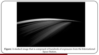
Figure: Hierarchically identified clusters

6. Signal and Image Processing
 SciPy allows us to read and write image files like JPEG and PNG images
without worrying too much about the file structure for color images.
 Below, we run through a simple illustration of working with image files to
make a nice image (see Figure) from the International Space Station (ISS).
 Refer StackedImage.py
 The JPG images in the Python environment are NumPy arrays with (426, 640,
3), where the three layers are red, green, and blue, respectively.
 In the original stacked image, seeing the star trails above Earth is nearly
impossible.

Figure: A stacked image that is composed of hundreds of exposures from the International
Space Station.

 We modify the previous example to enhance the star trails as shown in Figure
 Refer StarTrails.py
 When dealing with images without SciPy, you have to be more concerned
about keeping the array values in the right format when saving them as image
files. SciPy deals with that nicely and allows us to focus on processing the
images and obtaining our desired effects.

7. Sparse Matrices
 With NumPy we can operate with reasonable speeds on arrays containing 106
elements.
 Once we go up to 107 elements, operations can start to slowdown and Python’s
memory will become limited, depending on the amount of RAM available.
 What’s the best solution if you need to work with an array that is far larger—
say, 1010 elements? If these massive arrays primarily contain zeros, then you’re
in luck, as this is the property of sparse matrices.
 If a sparse matrix is treated correctly, operation time and memory usage can
go down drastically. The simple example below illustrates this.

 Refer SparseMatrices.py
 The memory allotted to the NumPy array and sparse matrix were 68MB and 0.68MB,
respectively.
 In the same order, the times taken to process the Eigen commands were 36.6 and 0.2
seconds on my computer.
 This means that the sparse matrix was 100 times more memory efficient and the Eigen
operation was roughly 150 times faster than the non-sparse cases.
 In 2D and 3D geometry, there are many sparse data structures used in fields like
engineering, computational fluid dynamics, electromagnetism, thermodynamics, and
acoustics.
 Non-geometric instances of sparse matrices are applicable to optimization, economic
modeling, mathematics and statistics, and network/graph theories.

 Using scipy.io, you can read and write common sparse matrix file formats such
as Matrix Market and Harwell-Boeing, or load MatLab files.
 This is especially useful for collaborations with others who use these data
formats.

8. Reading and Writing Files Beyond NumPy
 NumPy provides a good set of input and output capabilities with ASCII files.
Its binary support is great if you only need to share information to be read
from one Python environment to another.
 But what about more universally used binary file formats?
 If you are using Matlab or collaborating with others who are using it, then as
briefly mentioned in the previous section, it is not a problem for NumPy to
read and write Matlab-supported files (using scipy.io.loadmat and
scipy.savemat).

 In fields like astronomy, geography, and medicine, there is a programming
language called IDL.
 It saves files in a binary format and can be read by NumPy using a built-in
package called scipy.io.readsav. It is a flexible and fast module, but it
does not have writing capabilities.
 Last but not least, you can query, read, and write Matrix Market files. These are
very commonly used to share matrix data structures that are written in ASCII
format.
 This format is well supported in other languages like C, Fortran, and Matlab,
so it is a good format to use due to its universality and user readability. It is
also suitable for sparse matrices.

1. Scikit-Image
 SciPy’s ndimage class contains many useful tools for processingmulti-
dimensional data, such as basic filtering (e.g., Gaussian smoothing), Fourier
transform, morphology (e.g., binary erosion), interpolation, and
measurements.
 From those functions we can write programs to execute more complex
operations. Scikit-image has fortunately taken on the task of going a step
further to provide more advanced functions that we may need for scientific
research.
 These advanced and high-level modules include color space conversion, image
intensity adjustment algorithms, feature detections, filters for sharpening and
denoising, read/write capabilities, and more.

(i) Dynamic Threshold
 A common application in imaging science is segmenting image components
from one another, which is referred to as thresholding.
 The classic thresholding technique works well when the background of the
image is flat. Unfortunately, this situation is not the norm; instead, the
background visually will be changing throughout the image.
 Hence, adaptive thresholding techniques have been developed, and we can
easily utilize them in scikit-image.
 In the following example, we generate an image with a non-uniform
background that has randomly placed fuzzy dots throughout (see Figure).

 Then we run a basic and adaptive threshold function on the image to see how
well we can segment the fuzzy dots from the background.
 Refer Threshold.py
 In this case, as shown in Figure, the adaptive thresholding technique (right
panel) obviously works far better than the basic one (middle panel).
 Most of the code above is for generating the image and plotting the output for
context.
 The actual code for adaptively thresholding the image took only two lines.

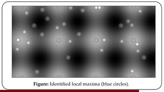
Figure: Illustration of thresholding.

(ii) Local Maxima
 Approaching a slightly different problem, but with a similar setup as before,
how can we identify points on a non-uniform background to obtain their pixel
coordinates?
 Here we can use skimage.morphology.is_local_maximum, which only
needs the image as a default input. The function works surprisingly well; see
Figure, where the identified maxima are circled in blue.
 Refer LocalMaxima.py

Figure: Identified local maxima (blue circles).

 If you look closely at the figure, you will notice that there are identified
maxima that do not point to fuzzy sources but instead to the background
peaks.
 These peaks are a problem, but by definition this is what
skimage.morphology.is_local_maximum will find.
 How can we filter out these “false positives”? Since we have the coordinates of
the local maxima, we can look for properties that will differentiate the sources
from the rest.
 The background is relatively smooth compared to the sources, so we could
differentiate them easily by standard deviation from the peaks to their local
neighboring pixels.

 How does scikit-image fare with real-world research problems? Quite well, in
fact. In astronomy, the flux per unit area received from stars can be measured
in images by quantifying intensity levels at their locations—a process called
photometry.
 Photometry has been done for quite some time in multiple programming
languages, but there is no defacto package for Python yet. The first step in
photometry is identifying the stars.
 In the following example, we will use is_local_maximum to identify sources
(hopefully stars) in a stellar cluster called NGC 3603 that was observed with
the Hubble Space Telescope.
 Note that one additional package, PyFITS1 is used here. It is a standard
astronomical package for loading binary data stored in FITS2 format.

 The skimage.morphology.is_local_maximum function returns over
30,000 local maxima in the image, and many of the detections are false
positives.
 We apply a simple threshold value to get rid of any maxima peaks that have a
pixel value below 0.5 (from the normalized image) to bring that number down
to roughly 200.
 There are much better ways to filter out non-stellar maxima (e.g., noise), but
we will still stick with the current method for simplicity. In Figure we can see
that the detections are good overall.
 Refer SourceIdentification.py

2. Scikit-Learn
 Possibly the most extensive scikit is scikit-learn. It is an easy-to-use machine
learning bundle that contains a collection of tools associated with supervised
and unsupervised learning.
 Some of you may be asking, “So what can machine learning help me do that I
could not do before?” One word: predictions.
 Let us assume that we are given a problem where there is a good sample of
empirical data at hand: can predictions be made about it? To figure this out,
we would try to create an analytical model to describe the data, though that
does not always work due to complex dependencies.
 But what if you could feed that data to a machine, teach the machine what is
good and bad about the data, and then let it provide its own predictions? That
is what machine learning is. If used right, it can be very powerful.

(i) Linear Regression
 If we are dealing with data that has a higher number of dimensions, how do
we go about a linear regression solution?
 Scikit-learn has a large number of tools to do this, such as Lasso and ridge
regression.
 For now we will stick with the ordinary least squares regression function,
which solves mathematical problems of the form
 where 𝜔 is the set of coefficients

 The number of coefficients depends on the number of dimensions in the data,
𝑁 𝑐𝑜𝑒𝑓𝑓 = 𝑀𝐷 − 1, where 𝑀 > 1 and is an integer.
 In the example below we are computing the linear regression of a plane in 3D
space, so there are two coefficients to solve for.
 Here we show how to use Linear Regression to train the model with data,
approximate a best fit, give a prediction from the data, and test other data
(test) to see how well it fits the model. A visual output of the linear regression
is shown in Figure.
 Refer Regression.py
 This Linear Regression function can work with much higher dimensions, so
dealing with a larger number of inputs in a model is straightforward.

Figure: A scikit-learn linear regression in 3D space.

(ii) Clustering
 SciPy has two packages for cluster analysis with vector quantization (kmeans)
and hierarchy. The kmeans method was the easier of the two for
implementing and segmenting data into several components based on their
spatial characteristics.
 Scikit-learn provides a set of tools to do more cluster analysis that goes
beyond what SciPy has. For a suitable comparison to the kmeans function in
SciPy, the DBSCAN algorithm is used in the following example.
 DBSCAN works by finding core points that have many data points within a
given radius

 Once the core is defined, the process is iteratively computed until there are no
more core points definable within the maximum radius? This algorithm does
exceptionally well compared to kmeans where there is noise present in the
data.
 Refer DBSCAN.py
 Nearly all the data points originally defined to be part of the clusters are
retained, and the noisy background data points are excluded (see Figure).
 This highlights the advantage of DBSCAN over kmeans when data that should
not be part of a cluster is present in a sample.
 This obviously is dependent on the spatial characteristics of the given
distributions.

Figure: An example of how the DBSCAN algorithm excels over the
vector quantization package in SciPy.

References
1. Bressert, E. (2012). SciPy and NumPy: an overview for developers. O’REILLY.

Computation Using Scipy, Scikit Image, Scikit Learn

Recommended

More Related Content

Similar to Computation Using Scipy, Scikit Image, Scikit Learn (20)

More from Prabu U (20)

Recently uploaded (20)

Computation Using Scipy, Scikit Image, Scikit Learn