Discrete random variable.

Discrete Random Variables
Slide 1

Shakeel Nouman
M.Phil Statistics

Random Variables By Shakeel Nouman M.Phil Statistics Govt. College University Lahore, Statistical Officer

3








Slide 2

Random Variables

Using Statistics
Expected Values of Discrete Random Variables
The Binomial Distribution
Other Discrete Probability Distributions
Continuous Random Variables
Using the Computer
Summary and Review of Terms


3-1 Using Statistics

Slide 3

Consider the different possible orderings of boy (B) and girl (G) in
four sequential births. There are 2*2*2*2=24 = 16 possibilities, so
the sample space is:
BBBB
BBBG
BBGB
BBGG

BGBB
BGBG
BGGB
BGGG

GBBB
GBBG
GBGB
GBGG

GGBB
GGBG
GGGB
GGGG

If girl and boy are each equally likely [P(G)=P(B) = 1/2], and the
gender of each child is independent of that of the previous child,
then the probability of each of these 16 possibilities is:
(1/2)(1/2)(1/2)(1/2) = 1/16.

Random Variables

Slide 4

Now count the number of girls in each set of four sequential births:
BBBB
BBBG
BBGB
BBGG
•
•
•

(0)
(1)
(1)
(2)

BGBB
BGBG
BGGB
BGGG

(1)
(2)
(2)
(3)

GBBB
GBBG
GBGB
GBGG

(1)
(2)
(2)
(3)

GGBB
GGBG
GGGB
GGGG

(2)
(3)
(3)
(4)

Notice that:
each possible outcome is assigned a single numeric value,
all outcomes are assigned a numeric value, and
the value assigned varies over the outcomes.

The count of the number of girls is a random variable:
A random variable, X, is a function that assigns a single, but variable, value to
each element of a sample space.

Random Variables (Continued)

Slide 5

0

BBBB
BGBB
GBBB
BBBG
BBGB
GGBB
GBBG
BGBG
BGGB
GBGB
BBGG
BGGG
GBGG
GGGB
GGBG
GGGG

1

X
2

3
4
Sample Space

Points on the
Real Line


Random Variables (Continued)

Slide 6

Since the random variable X = 3 when any of the four outcomes BGGG, GBGG,
GGBG, or GGGB occurs,
P(X = 3) = P(BGGG) + P(GBGG) + P(GGBG) + P(GGGB) = 4/16
The probability distribution of a random variable is a table that lists the
possible values of the random variables and their associated probabilities.
P(x)
1/16
4/16
6/16
4/16
1/16
16/16=1

P r o b a b ility D is trib u tio n o f t h e N u m b e r o f G irls in F o u r B ir th s
0 .4

0 .3 7 5 0

0 .3
0 .2 5 0 0

P(x)

x
0
1
2
3
4

0 .2 5 0 0

0 .2

0 .1
0 .0 6 2 5
0

0 .0 6 2 5
1

2

3

4

N u m b e r o f g irls , x


Example 3-1

Slide 7

Consider the experiment of tossing two six-sided dice. There are 36 possible
outcomes. Let the random variable X represent the sum of the numbers on
the two dice:

3
1,3
2,3
3,3
4,3
5,3
6,3

4
1,4
2,4
3,4
4,4
5,4
6,4

5
1,5
2,5
3,5
4,5
5,5
6,5

6
1,6
2,6
3,6
4,6
5,6
6,6

7
8
9
10
11
12

P(x)*
1/36
2/36
3/36
4/36
5/36
6/36
5/36
4/36
3/36
2/36
1/36
1

Po a tyDstrib tio u w ic
r b bili i u nofSmofT oD e
0.17

0.12

p(x)

1,1
2,1
3,1
4,1
5,1
6,1

2
1,2
2,2
3,2
4,2
5,2
6,2

x
2
3
4
5
6
7
8
9
10
11
12

0.07

0.02
2

3

4

5

6

7

8

9

10

x

* Note that: P(x)  (6  (7  x) 2 ) / 36


11

12

Example 3-2

Slide 8

Probability Distribution of the Number of Switches
P(x)
0.1
0.2
0.3
0.2
0.1
0.1
1

TePr ba yD b o fth u berofS itc es
h o bilit istri uti no eNm w h
0.4

0.3

P(x)

x
0
1
2
3
4
5

0.2

0.1

0.0
0

1

2

3

4

5

x

Probability of more than 2 switches:
P(X > 2) = P(3) + P(4) + P(5) = 0.2 + 0.1 + 0.1 = 0.4
Probability of at least 1 switch:
P(X ³ 1) = 1 - P(0) = 1 - 0.1 = .9

Discrete and Continuous Random
Variables





Slide 9

A discrete random variable:
 has a countable number of possible values
 has discrete jumps (or gaps) between successive values
has measurable probability associated with individual values
 counts

A continuous random variable:
 has an uncountably infinite number of possible values
 moves continuously from value to value
 has no measurable probability associated with each value
measures (e.g.: height, weight, speed, value, duration, length)


Rules of Discrete Probability
Distributions

Slide 10

The probability distribution of a discrete
random variable X must satisfy the following
two conditions.
1. P(x)  0 for all values of x.
2.

 P(x)  1
all x

Corollary: 0  P( X )  1


Cumulative Distribution
Function

Slide 11

The cumulative distribution function, F(x), of a discrete
random variable X is:
F(x)  P( X  x) 

 P(i)

all i  x

P(x)
0.1
0.2
0.3
0.2
0.1
0.1

F(x)
0.1
0.3
0.6
0.8
0.9
1.0

1

Cumulative Prob ability Distribution of the Numb er of Switche s
1 .0
0 .9
0 .8
0 .7

F(x)

x
0
1
2
3
4
5

0 .6
0 .5
0 .4
0 .3
0 .2
0 .1
0 .0
0

1

2

3

4

5

x


Cumulative Distribution
Function

Slide 12

The probability that at most three switches will occur:
The P ro b a bility Tha t at Mo s t T hre e S witc he s W ill O c c ur

P(x)
0.1
0.2
0.3
0.2
0.1
0.1

F(x)
0.1
0.3
0.6
0.8
0.9
1.0

0 .4

P( X  3)  F(3)
0 .3

P (x)

x
0
1
2
3
4
5

0 .2

0 .1

1
0 .0
0

1

2

3

4

5

x

Note: P(X < 3) = F(3) = 0.8 = P(0) + P(1) + P(2) + P(3)

Using Cumulative Probability
Distributions (Figure 3-8)

Slide 13

The probability that more than one switch will occur:
The Probability That More than One Switch Will Occur

P(x)
0.1
0.2
0.3
0.2
0.1
0.1

F(x)
0.1
0.3
0.6
0.8
0.9
1.0

0 .4

0 .3

P ( x)

x
0
1
2
3
4
5

P( X  1  1 F(1
)
)

F(1
)

0 .2

0 .1

1
0 .0
0

1

2

3

4

5

x

Note: P(X > 1) = P(X > 2) = 1 – P(X < 1) = 1 – F(1) = 1 – 0.3 = 0.7

Using Cumulative Probability
Distributions (Figure 3-9)

Slide 14

The probability that anywhere from one to three
switches will occur:
The Probability That Anywhere from One to Three Switches Will Occur

P(x)
0.1
0.2
0.3
0.2
0.1
0.1

F(x)
0.1
0.3
0.6
0.8
0.9
1.0
1

0 .4

F(1 X  3)  F(3)  F(0)
F(3)

0 .3

P (x)

x
0
1
2
3
4
5

0 .2

F(0)
0 .1

0 .0
0

1

2

3

4

5

x

Note: P(1 < X < 3) = P(X < 3) – P(X < 0) = F(3) – F(0) = 0.8 – 0.1 = 0.7

3-2 Expected Values of Discrete
Random Variables
The mean of a probability distribution is a
measure of its centrality or location, as is the
mean or average of a frequency distribution. It is
a weighted average, with the values of the
random variable weighted by their probabilities.

0

1

2

3

Slide 15

4

5

2.3

The mean is also known as the expected value (or expectation) of a random
variable, because it is the value that is expected to occur, on average.
The expected value of a discrete random
variable X is equal to the sum of each
value of the random variable multiplied by
its probability.

m  E ( X )   xP ( x )

x
P(x)
xP(x)
0
0.1
0.0
1
0.2
0.2
2
0.3
0.6
3
0.2
0.6
4
0.1
0.4
5
0.1
0.5
1.0
2.3 = E(X) = m

all x


A Fair Game

Slide 16

Suppose you are playing a coin toss game in which you are
paid $1 if the coin turns up heads and you lose $1 when the
coin turns up tails. The expected value of this game is E(X) =
0. A game of chance with an expected payoff of 0 is called a
fair game.
x P(x) xP(x)
-1 0.5
-0.50
1 0.5
0.50
1.0
0.00 = E(X)=m

-1

0

1


Expected Value of a Function of
a Discrete Random Variables

Slide 17

The expected value of a function of a discrete random variable X is:
E [ h ( X )]   h ( x ) P ( x )
all x

Example 3-3: Monthly sales of a certain
product are believed to follow the given
probability distribution. Suppose the
company has a fixed monthly production
cost of $8000 and that each item brings
$2. Find the expected monthly profit
h(X), from product sales.
E [ h ( X )]   h ( x ) P ( x )  5400
all x

of items, x
5000
6000
7000
8000
9000

Number
P(x) xP(x)
h(x) h(x)P(x)
0.2 1000 2000
400
0.3 1800 4000
1200
0.2 1400 6000
1200
0.2 1600 8000
1600
0.1
900 10000
1000
1.0 6700
5400

Note: h(X) = 2X – 8000 where X = # of items sold

The expected value of a linear function of a random variable is:
E(aX+b)=aE(X)+b
In this case: E(2X8000)2E(X)8000(2)(6700)80005400

Variance and Standard Deviation
of a Random Variable

Slide 18

The variance of a random variable is the expected
squared deviation from the mean:
s

2

 V ( X )  E [( X  m ) 2 ] 



(x  m ) 2 P(x)

a ll x


 

 E ( X 2 )  [ E ( X )] 2    x 2 P ( x )     xP ( x ) 
 a ll x
  a ll x


2

The standard deviation of a random variable is the
square root of its variance:
s  SD( X )  V ( X )

Variance and Standard Deviation of a Slide 19
Random Variable – using Example 3-2
s 2 = V ( X ) = E[( X - m)2 ]

Table 3-8
Switches, x
0
1
2
3
4
5

m
Recall:

P(x)
0.1
0.2
0.3
0.2
0.1
0.1

Number of
xP(x) (x-m)
(x-m)2 P(x-m)2
0.0
-2.3
5.29
0.529
0.2
-1.3
1.69
0.338
0.6
-0.3
0.09
0.027
0.6
0.7
0.49
0.098
0.4
1.7
2.89
0.289
0.5
2.7
7.29
0.729
2.3
2.010

= 2.3.

x2P(x)
0.0
0.2
1.2
1.8
1.6
2.5
7.3

= å ( x - m)2 P( x) = 2.01
all x
= E( X 2 ) - [ E( X )]2
2
é
ù é
ù
= ê å x2 P( x)ú - ê å xP( x)ú
ëall x
û ëall x
û
= 7.3 - 2.32 = 2.01


Variance of a Linear Function of a
Random Variable

Slide 20

The variance of a linear function of a random variable is:

V(a X b)  a2V( X)  a2s2
Example 3-3:
Number
of items, x P(x) xP(x)
x2 P(x)
5000
0.2 1000 5000000
6000
0.3 1800 10800000
7000
0.2 1400 9800000
8000
0.2 1600 12800000
9000
0.1
900 8100000
1.0 6700
46500000

s2 V(X)
 E ( X 2 )  [ E ( X )]2
2

 

2
  x P( x )    xP( x )
all x
 all x

 46500000  ( 67002 )  1610000

s  SD( X )  1610000  1268.86

V (2 X  8000)  (2 2 )V ( X )
 ( 4)(1610000)  6440000

s ( 2 x  8000)  SD(2 x  8000)
 2s x  (2)(1268.86)  2537.72


Some Properties of Means and
Variances of Random Variables

Slide 21

The mean or expected value of the sum of random variables
is the sum of their means or expected values:

m( XY)  E( X Y)  E( X)  E(Y)  mX  mY

For example: E(X) = $350 and E(Y) = $200
E(X+Y) = $350 + $200 = $550

The variance of the sum of independent random variables is
the sum of their variances:
s 2 ( X Y )  V ( X  Y)  V ( X ) V (Y)  s 2 X  s 2 Y
if and only if X and Y are independent.

For example: V(X) = 84 and V(Y) = 60

V(X+Y) = 144


Chebyshev’s Theorem Applied to
Probability Distributions

Slide 22

Chebyshev’s Theorem applies to probability distributions just
as it applies to frequency distributions.
For a random variable X with mean m, standard deviation s,
and for any number k > 1:
1
P( X  m  ks)  1 2
k
1

At
least

1
1 3
 1    75%
2
4 4
2

1
1 8
1  2  1    89%
9 9
3
1
1 15
1 2  1

 94%
16 16
4

2
Lie
within

3
4

Standard
deviations
of the mean


Using the Template to Calculate
statistics of h(x)

Slide 23


3-3 Bernoulli Random Variable

Slide 24

• If an experiment consists of a single trial and the outcome of the
trial can only be either a success* or a failure, then the trial is
called a Bernoulli trial.
• The number of success X in one Bernoulli trial, which can be 1 or
0, is a Bernoulli random variable.
• Note: If p is the probability of success in a Bernoulli experiment,
the E(X) = p and V(X) = p(1 – p).

* The

terms success and failure are simply statistical terms, and do not have positive or
negative implications. In a production setting, finding a defective product may be termed
a “success,” although it is not a positive result.


The Binomial Random Variable

Slide 25

Consider a Bernoulli Process in which we have a sequence of n identical
trials satisfying the following conditions:
1. Each trial has two possible outcomes, called success *and failure.
The two outcomes are mutually exclusive and exhaustive.
2. The probability of success, denoted by p, remains constant from trial
to trial. The probability of failure is denoted by q, where q = 1-p.
3. The n trials are independent. That is, the outcome of any trial does
not affect the outcomes of the other trials.
A random variable, X, that counts the number of successes in n Bernoulli
trials, where p is the probability of success* in any given trial, is said to
follow the binomial probability distribution with parameters n (number
of trials) and p (probability of success). We call X the binomial random
variable.
* The terms success and failure are simply statistical terms, and do not have positive or negative implications. In a
production setting, finding a defective product may be termed a “success,” although it is not a positive result.

Binomial Probabilities
(Introduction)

Slide 26

Suppose we toss a single fair and balanced coin five times in succession,
and let X represent the number of heads.
There are 25 = 32 possible sequences of H and T (S and F) in the sample space for this
experiment. Of these, there are 10 in which there are exactly 2 heads (X=2):
HHTTT HTHTH HTTHT HTTTH THHTT THTHT THTTH TTHHT TTHTH TTTHH

The probability of each of these 10 outcomes is p3q3 = (1/2)3(1/2)2=(1/32), so the
probability of 2 heads in 5 tosses of a fair and balanced coin is:

P(X = 2) = 10 * (1/32) = (10/32) = .3125
10

(1/32)

Number of outcomes
with 2 heads

Probability of each
outcome with 2 heads


Binomial Probabilities (continued)

Slide 27

P(X=2) = 10 * (1/32) = (10/32) = .3125
Notice that this probability has two parts:
10

(1/32)

Number of outcomes
with 2 heads

Probability of each
outcome with 2 heads

In general:
1. The probability of a given sequence
of x successes out of n trials with
probability of success p and
probability of failure q is equal to:

pxq(n-x)

2. The number of different sequences of n trials that
result in exactly x successes is equal to the number
of choices of x elements out of a total of n elements.
This number is denoted:

n!
 n
nCx    
 x x!( n  x)!


The Binomial Probability
Distribution
The binomial probability distribution:

n!
 n x ( n  x )
P( x)    p q

px q ( n x)
x!( n  x)!
 x

where :
p is the probability of success in a single trial,
q = 1-p,
n is the number of trials, and
x is the number of successes.

N u m b er o f
su ccesses, x
0
1
2
3

n

Slide 28

P ro b ab ility P (x )
n!
p 0 q (n 0)
0 !( n  0 ) !
n!
p 1 q ( n  1)
1 !( n  1 ) !
n!
p 2 q (n 2)
2 !( n  2 ) !
n!
p 3 q (n 3)
3 !( n  3 ) !

n!
p n q (n n)
n !( n  n ) !
1 .0 0


The Cumulative Binomial
Probability Table (Table 1,
Appendix C)

Slide 29

n=5
p
x

0.01

0.05

0.10

0.20

0.30

0.40

0.50

0.60

0.70

0.80

0.90

0.95

0.99

0

.951

.774

.590

.328

.168

.078

.031

.010

.002

.000

.000

.000

.000

1

.999

.977

.919

.737

.528

.337

.187

.087

.031

.007

.000

.000

.000

2

1.000

.999

.991

.942

.837

.683

.500

.317

.163

.058

.009

.001

.000

3

1.000

1.000

1.000

.993

.969

.913

.813

.663

.472

.263

.081

.023

.001

4

1.000

1.000

1.000

1.000

.998

.990

.969

.922

.832

.672

.410

.226

.049

h

F(h)

P(h)

0

0.031 0.031

1

0.187 0.156

2

0.500 0.313

3

0.813 0.313

4

0.969 0.156

5

1.000 0.031
1.000

Cumulative Binomial
Probability Distribution and
Binomial Probability
Distribution of H,the
Number of Heads
Appearing in Five Tosses of
a Fair Coin

Deriving Individual Probabilities
from Cumulative Probabilities
F (x )  P ( X  x ) 

 P(i )

all i  x

P(X) = F(x) - F(x - 1)
For example:
P (3)  F (3)  F (2)
 .813 .500
 .313


Calculating Binomial
Probabilities Example

Slide 30

60% of Brooke shares are owned by LeBow. A random sample
of 15 shares is chosen. What is the probability that at most
three of them will be found to be owned by LeBow?
n=15

0
1
2
3
4
...

.50
.000
.000
.004
.018
.059
...

p
.60
.000
.000
.000
.002
.009
...

.70
.000
.000
.000
.000
.001
...

F (x )  P ( X  x ) 

 P (i )

all i  x

F ( 3)  P ( X  3)  .002


Mean, Variance, and Standard Slide 31
Deviation of the Binomial Distribution
Mean of a binomial distribution:

m  E ( X )  np

For example, if H counts the number of
heads in five tosses of a fair coin :

Variance of a binomial distribution:

m  E ( H )  (5)(.5)  2.5
H

s  V ( X )  npq
2

s  V ( H )  (5)(.5)(.5)  1.25
2

H

Standard deviation of a binomial distribution:

s = SD(X) = npq

s  SD( H )  1.25  1.118
H


Calculating Binomial Probabilities
using the Template

Slide 32


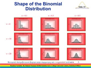
Shape of the Binomial
Distribution
p  0.1

Slide 33

p  0.3

Binomial Probability: n=4 p=0.1

p  0.5



0.6

0.5

0.5

0.4

0.4

0.4

0.3

P(x)

0.6

0.5

P(x)

0.7

0.6

n4

0.7

P(x)

0.7

0.3

0.2

0.2

0.1

0.1

0.0

0.2
0.1

0.0
0

1

2

3

0.3

0.0

4

0

1

2

x

3

4

0



4

0.4

0.4

0.3

0.3

0.3

P(x)

0.5

P(x)

P(x)

3


0.5

0.4

0.2

0.2

0.2

0.1

0.1

0.1

0.0

0.0
0

1

2

3

4

5

6

7

8

9 10

0.0
0

1

2

3

4

5

6

7

8

0

9 10

x


1

2

x


0.1

4

5
x

6

7

8

9 10

P(x)

0.2

0.1

0.0

3


0.2

P(x)

0.2

P(x)

n  20

2

x

0.5

n  10

1

x

0.1

0.0

0.0

0 1 2 3 4 5 6 7 8 9 1011121314151617181920

0 1 2 3 4 5 6 7 8 9 1011121314151617181920

0 1 2 3 4 5 6 7 8 9 1011121314151617181920

x

x

x

Binomial distributions become more symmetric as n increases and as p

.5.


3-5 Negative Binomial
Distribution

Slide 34

The negative binomial distribution is useful for determining the probability of the
number of trials made until the desired number of successes are achieved in a
sequence of Bernoulli trials. It counts the number of trials X to achieve the
number of successes s with p being the probability of success on each trial.

Negative Binomial Distribution :
P( X  x) 

( )
x 1
s 1

s

p (1  p )

( x  s)

The mean is : m 

s
p

The variance is : s

2



s (1  p )
p2


Negative Binomial Distribution Example
Example:
Suppose that the probability of a
manufacturing
process
producing a defective item is
0.05. Suppose further that the
quality of any one item is
independent of the quality of
any other item produced. If a
quality control officer selects
items at random from the
production line, what is the
probability
that the first
defective item is the eight item
selected.

Slide 35

Heres = 1, x = 8, and p = 0.05. Thus,

 8  1
P( X  8)  
0.05 (1  0.05)
1  1 
 0.0349
1

( 81 )


Calculating Negative Binomial
Probabilities using the Template

Slide 36


3-6 The Geometric Distribution

Slide 37

Within the context of a binomial experiment, in which the outcome of each of n
independent trials can be classified as a success (S) or a failure (F), the
geometric random variable counts the number of trials until the first success..
Geometric distribution:
x1
P ( x )  pq
where x = 1,2,3, . . . and p and q are the binomial parameters.
The mean and variance of the geometric distribution are:

m

1
p

s

2



q
2
p


The Geometric Distribution Example

Slide 38

Example:
A recent study indicates that Pepsi-Cola
has a market share of 33.2% (versus
40.9% for Coca-Cola). A marketing
research firm wants to conduct a new
taste test for which it needs Pepsi
P(1)  (.332)(.668)(11)  0332
.
drinkers. Potential participants for the
( 21)
test are selected by random screening of P(2)  (.332)(.668)
 0222
.
soft drink users to find Pepsi drinkers.
P(3)  (.332)(.668)( 31)  0148
.
What is the probability that the first
( 41)
 0.099
randomly selected drinker qualifies? P( 4)  (.332)(.668)
What’s the probability that two soft drink
users will have to be interviewed to find
the first Pepsi drinker? Three? Four?


Calculating Geometric
Distribution Probabilities using
the Template

Slide 39


3-7 The Hypergeometric
Distribution

Slide 40

The hypergeometric probability distribution is useful for determining the
probability of a number of occurrences when sampling without replacement. It
counts the number of successes (x) in n selections, without replacement, from a
population of N elements, S of which are successes and (N-S) of which are failures.

H ypergeom etric D istribution: The mean of the hypergeometric distribution is: m  np , where p 

 
 

 X n  x 
 N
 
 n
S

P(x) 

N  S

The variance is: s

2

 N  n  npq
 

 N  1


S
N

The Hypergeometric Distribution Example
Example:
Suppose that automobiles arrive at a
dealership in lots of 10 and that for
time and resource considerations,
only 5 out of each 10 are inspected
for safety. The 5 cars are randomly
chosen from the 10 on the lot. If 2
out of the 10 cars on the lot are below
standards for safety, what is the
probability that at least 1 out of the 5
cars to be inspected will be found not
meeting safety standards?

()

( )( )
() ()
 ( )
( ) ( ) ( )( )
() ()
 (10  2)


1  (5  1) 

2

P (1) 

2

4



10



5

2

10  2

1

5 2

2

2!

3



10



10

5

1! 1! 4 ! 4 !

5


 0.556
9

5! 5!

8

1

8!

10 !

10

5

P( 2) 

2!

8

1

Slide 41

5

8!

1! 1! 3 ! 5!
10 !



2
9

5! 5!

Thus, P(1) + P(2) =
0.556 + 0.222 = 0.778.


 0.222

Calculating Hypergeometric
Distribution Probabilities using
the Template


3-8 The Poisson Distribution

Slide 43

The Poisson probability distribution is useful for determining the probability of a
number of occurrences over a given period of time or within a given area or
volume.
That is, the Poisson random variable counts occurrences over a
continuous interval of time or space. It can also be used to calculate approximate
binomial probabilities when the probability of success is small (p£0.05) and the
number of trials is large (n³20).

Poisson D istribution :
m xe m
P( x) 
for x = 1,2,3,...
x!
where m is the mean of the distribution (which also happens to be the variance) and
e is the base of natural logarithms (e=2.71828...).


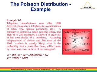
The Poisson Distribution Example
Example 3-5:
Telephone manufacturers now offer 1000
different choices for a telephone (as combinations
of color, type, options, portability, etc.). A
company is opening a large regional office, and
each of its 200 managers is allowed to order his
or her own choice of a telephone. Assuming
independence of choices and that each of the
1000 choices is equally likely, what is the
probability that a particular choice will be made
by none, one, two, or three of the managers?

Slide 44

.2 0 e - .2
P ( 0) =
= 0.8187
0! .2
.21 e P (1) =
= 0.1637
1! - .2
.2 2 e
P (2) =
= 0.0164
2 !- .2
.2 3 e
P ( 3) =
= 0.0011
3!

n = 200 m = np = (200)(0.001) = 0.2
p = 1/1000 = 0.001


Calculating Poisson Distribution


The Poisson Distribution
(continued)
•

Slide 46

Poisson assumptions:
The probability that an event will occur in a
short interval of time or space is proportional
to the size of the interval.
In a very small interval, the probability that two
events will occur is close to zero.
The probability that any number of events will
occur in a given interval is independent of
where the interval begins.
The probability of any number of events
occurring over a given interval is independent
of the number of events that occurred prior to
the interval.

The Poisson Distribution
(continued)
m =1.5

m =1.0
0.4

0.3

0.3

)
P( x

0.4

P(x)

Slide 47

0.2

0.1

0.2

0.1

0.0

0.0
0

1

2

3

4

0

1

2

3

4

X

m =4

5

6

7

X

m =10

0.2

0.15

P (x)

P(x)

0.10
0.1

0.05

0.0

0.00
0

1

2

3

4

5

X

6

7

8

9

10

0 1 2 3 4 5 6 7 8 9 1011121314151617181920

X


Discrete and Continuous
Random Variables - Revisited

• A continuous random variable:

• A discrete random variable:

– measures (e.g.: height, weight,

–
–

possible values
has discrete jumps between
successive values
has measurable probability
associated with individual values
probability is height

For example:
Binomial
n=3 p=.5
P(x)
0.125
0.375
0.375
0.125
1.000

0.4
0.3

P(x
)

x
0
1
2
3

Binomial: n=3 p=.5

0.2
0.1
0.0
0

1

2

C1

3

–
–
–
–

speed, value, duration, length)
has an uncountably infinite
number of possible values
moves continuously from value to
value
has no measurable probability
associated with individual values
probability is area

For example:
In this case,
the
shaded
area epresents
the probability
that the task
takes between
2
and
3
minutes.

Minute s to Co mplete Tas k
0.3

0.2

P(x)

– counts occurrences
– has a countable number of
–

Slide 48

0.1

0.0
1

2

3

4

Minutes


5

6

From a Discrete to a Continuous
Distribution

Slide 49

The time it takes to complete a task can be subdivided into:
Half-Minute Intervals

Eighth-Minute Intervals

Quarter-Minute Intervals
M
inutes to Complete Task: Fourths of a Minute

Minute s to Complete Task: By Half-Minute s

M
inutes to Complete Task: Eighths of a M
inute

0.15

P(x)

P(x)

P(x)

0.10

0.05

0.00
0.01.0 1.5 2.0 2.5 3.0 3.5 4.0 4.5 5.0 5.5 6.0 6.5
.

0

M
inutes

1

2

3

4

5

6

7

0

1

2

Minute s

3

4

5

6

7

M
inutes

Or even infinitesimally small intervals:

f(z)

Minutes to Complete Task: Probability Density Function

0

1

2

3

4

5

6

When a continuous random variable has been subdivided into
infinitesimally small intervals, a measurable probability can
only be associated with an interval of values, and the
probability is given by the area beneath the probability density
function corresponding to that interval. In this example, the
shaded area represents P(2 £ X £ 3).

7

Minutes


3-9 Continuous Random
Variables

Slide 50

A continuous random variable is a random variable that can take on any value in an
interval of numbers.

The probabilities associated with a continuous random variable X are determined by the
probability density function of the random variable. The function, denoted f(x), has the
following properties.
1.
2.
3.

f(x) ³ 0 for all x.
The probability that X will be between two numbers a and b is equal to the area
under f(x) between a and b.
The total area under the curve of f(x) is equal to 1.00.

The cumulative distribution function of a continuous random variable:
F(x) = P(X £ x) =Area under f(x) between the smallest possible value of X (often -¥) and
the point x.


Probability Density Function and
Cumulative Distribution Function
F(x)
1
F(b)
F(a)
0
f(x)

}
a

b

Slide 51

P(a £ X £ b)=F(b) - F(a)

x
P(a £ X £ b) = Area under
f(x) between a and b
= F(b) - F(a)

0

a

b

x


3-10 Uniform Distribution

Slide 52

The uniform [a,b] density:

{

1/(a – b) for a £ X £ b
f(x)=
0 otherwise

E(X) = (a + b)/2; V(X) = (b – a)2/12

f(x)

Uniform [a, b]
Distribution

The entire area under f(x) =
1/(b – a) * (b – a) = 1.00
The area under f(x) from a1 to
b1 = P(a1£X£ b1)

a a
1

x

b
1

b

= (b1 – a1)/(b – a)


Uniform Distribution (continued)

Slide 53

The uniform [0,5] density:

{

1/5 for 0 £ X £ 5
f(x)=
0 otherwise

E(X) = 2.5

The entire area under
f(x) = 1/5 * 5 = 1.00

Uniform [0,5] Distribution
0.5
0.4

f(x)

0.3

The area under f(x) from 1 to 3
= P(1£X£3)

0.2
0.1
.0.0
-1

0

1

2

3

4

5

6

x

= (1/5)2 = 2/5

Calculating Uniform Distribution


3-11 Exponential Distribution

Slide 55

E xp o n e ntial Dis trib utio n: l = 2

The exponential random variable measures
the time between two occurrences that have
a Poisson distribution.

2

Exponential distribution:
f(x)

The density function is:
f (x)  lelx for x  0, l  0

1

1
The mean and standard deviation are both equal to .

l

The cumulative distribution function is:
F(x)  1  elx for x  0.

0
0

1

2

3

Time


Exponential Distribution Example

Slide 56

Example
The time a particular machine operates before breaking down (time between
breakdowns) is known to have an exponential distribution with parameter l = 2. Time is
measured in hours. What is the probability that the machine will work continuously for
at least one hour? What is the average time between breakdowns?

F (x ) = 1 - e - l x Þ P( X ³ x ) = e - l x
P ( X ³ 1) = e ( - 2 )(1)
=.1353

E(X ) =

1 1
= =.5
l 2


Calculating Exponential Distribution


Name
Religion
Domicile
Contact #
E.Mail
M.Phil (Statistics)

Shakeel Nouman
Christian
Punjab (Lahore)
0332-4462527. 0321-9898767
sn_gcu@yahoo.com
sn_gcu@hotmail.com
GC University, .
(Degree awarded by GC University)

M.Sc (Statistics)
Statitical Officer
(BS-17)
(Economics & Marketing
Division)

GC University, .
(Degree awarded by GC University)

Livestock Production Research Institute
Bahadurnagar (Okara), Livestock & Dairy Development
Department, Govt. of Punjab


Discrete random variable.

Recommended

More Related Content

What's hot (20)

Viewers also liked (8)

Similar to Discrete random variable. (20)

More from Shakeel Nouman (19)

Recently uploaded (20)

Discrete random variable.