SlideShare a Scribd company logo
Variational Autoencoders
for Image Generation
Steven Flores, sflores@compthree.com
Do you recognize these people?
Computer-generated images
No, you don’t. All images were generated by a random seed.
From “Progressive Growing of GANs for Improved Quality, Stability, and
Variation,” https://arxiv.org/abs/1710.10196.
Applications
● Image editing
From “Unpaired Image-to-Image Translation using Cycle-Consistent
Adversarial Networks,” https://arxiv.org/abs/1703.10593
Applications
● Style transfer
From “Unpaired Image-to-Image Translation using Cycle-Consistent
Adversarial Networks,” https://arxiv.org/abs/1703.10593
Applications
● Pose interpolation
From “Representation Learning by Rotating Your Faces,”
https://arxiv.org/abs/1705.11136
GeneratedInput
Applications
● Image repair
From “Context Encoders: Feature Learning by Inpainting,”
https://arxiv.org/abs/1604.07379
Applications
● Image synthesis
From “High-Resolution Image Synthesis and Semantic Manipulation with
Conditional GANs,” https://arxiv.org/abs/1711.11585
Contents
● Part 1: A survey of generative models in computer vision
● Part 2: From autoencoders to variational autoencoders
● Part 3: A Bayesian approach to variational autoencoders
Part 1
A survey of generative
models in computer vision
PixelRNN
● Generate an image pixel-by-pixel from the top-left corner going right/down.
● Each pixel value (red) depends only on
previous pixel values (blue).
● Pixel-value dependency is modeled with a
recurrent neural network, with parameters .
● Probability of pixel value
at site is computed in a final softmax layer.
● Probability of generating a particular image is
● Learning objective: maximize over training data .TL(θ) =
1
|T | ∑
x∈T
log pθ(x)
pθ(x) =
n
∏
i,j=1
pθ(xi,j | xi−1,j, xi,j−1)
pθ(xi,j | xi−1,j, xi,j−1) xi,j
x
θ
i, j
Generative Adversarial Network (GAN)
Fake Image
Random
Noise
=
Real
Image
Generator Discriminator
“Real” Label
“Fake” Label
Variational Autoencoder
A Bayesian twist on a lossy compression algorithm called an “autoencoder.”
Encoded Data
Encoder Decoder
Input Data Reconstructed Data
Latent
Space
σ2
1
σ2
2
μ1
μ2 Diagonal
Multivariate
Gaussian
Mean, Variance
Random Sample
Part 2
From autoencoders
to variational autoencoders
The autoencoder (AE)
● Learn a low-dimensional representation of high-dimensional data.
● Macro-architecture comprises an encoder followed by a decoder.
Encoder Decoder
low-dimensional
“latent" space
compressed
representation
E(x) reconstructed
data
original high-dimensional
vector space
D(E(x))
high-dimensional
vector space
original
datapoint
x
AE microarchitecture
● The encoder and decoder are usually neural networks:
● Layers are often fully connected or convolutional (for image data):
Encoded Data
Encoder Decoder
Input Data Reconstructed Data
Latent
Space
AE learning objective
● An AE learns by minimizing the objective function
where is our set of training data and is a “distance function.”
● Update weights in the encoder and decoder via gradient descent.
L =
1
|T| ∑
x∈T
d(x, D(E(x))
T d
E D
AE model evaluation
● An AE does well if loss, summed over a distinct validation set is small.
● Other ways of measuring quality are the “inception score” for image data,
mode coverage to measure output diversity, and interpolation methods.
V
L =
1
|V | ∑
x∈V
d(x, D(E(x))
Generated images from BigGAN
(a GAN, not an AE) which contribute
to this model’s state-of-the-art high
inception score of 166.3
From “Large Scale GAN Training for
High Fidelity Natural Image Synthesis”,
https://arxiv.org/abs/1809.11096
AE with MNIST
● MNIST is a famous dataset of 70,000 28 x 28 images of handwritten digits.
● Train an AE to compress digits to a 2-D latent space.
28 x 28
= 784
500 250 2
28 x 28
= 784
500250
Encoder Decoder
Latent
Space
All layers fully connected
AE digit reconstruction
AE with celebA
● CelebA is a dataset of over 200,000 images of celebrity faces.
● Train an AE to compress face images to a 100-D latent space.
100
64 x
64 x
3
4 x
4 x
256
4096
8 x
8 x
128
32 x
32 x
32
4 x 4 x 32
conv.
4 x 4 x 64
conv. 16 x
16 x
64
4 x 4 x 128
conv.
4 x 4 x 256
conv.
flatten
4096
32 x
32 x
32
64 x
64 x
3
16 x
16 x
64
4 x
4 x
256
4 x 4 x 256
deconv.
4 x 4 x 128
deconv. 8 x
8 x
128
4 x 4 x 64
deconv.
4 x 4 x 32
deconv.
4 x 4 x 3
deconv.
fully connectedfully connected
AE face reconstruction
Rightward and counting from one, odd col. = original, even col. = reconstruction.
AE data generation?
In an autoencoder, drop the encoder and feed the decoder a random sample.
Decoder
low-dimensional
“latent" space
random
sample
z generated
data
original high-dimensional
vector space
D(z)
Output quality
● What we want: “fake” data that looks like our training data.
● What we get: “garbage” if the random sampling is not done right.
Decoderz
Decoderz
AE digit generation
AE digit generation
Fake random handwritten digits generated by “decoding” the lattice sites.
AE digit generation
As before, but now decoding a “great circle” slicing a 10-D “red” hypersphere.
AE face generation
Generated from normal random samples using the training mean and variance.
AE limitations
● Encoded representations optimize for data reconstruction, not generation.
● Encoding clusters have irregular shape, which make them hard to sample.
● As a result, random generation of good imitation data is hard to do.
The encodings we got. The encodings we want.
Variational autoencoders (VAE)
A variational autoencoder (VAE) is an AE with two adaptations.
● Encoder maps datapoints to probability distributions.
● Add a new “KL-divergence” term to the loss function during training.
Encoded Data
Encoder Decoder
Input Data Reconstructed Data
Latent
Space
σ2
1
σ2
2
μ1
μ2 Diagonal
Multivariate
Gaussian
Mean, Variance
Random Sample
VAE learning objective
● KL-divergence measures “distance” between two probability distributions.
The KL term in encourages datapoints to map near to unit-Gaussians.
● Update weights in the encoder and decoder via gradient descent.E D
L =
1
|T | ∑
x∈T
d(x, D(E(x)) + KL(𝒩(μ(x), σ(x)2
) || 𝒩(0,1))
L
VAE digit reconstruction
VAE digit generation
Fake random handwritten digits generated by “decoding” the lattice sites.
VAE digit generation
As before, but now decoding a “great circle” slicing a 10-D “red” hypersphere.
VAE digit generation
AE vs VAE digit generation
left = AE generated digits, right = VAE generation digits (10-D latent space).
VAE face reconstruction
Rightward and counting from one, odd col. = original, even col. = reconstruction.
VAE face generation
Generated from unit-normal random samples.
AE vs VAE face reconstruction
left = original, middle = AE reconstruction, right = VAE reconstruction.
left = AE face generation, right = VAE face generation.
AE vs VAE face generation
VAE face interpolation
We can also gradually add features to faces:
● Find the center of mass of all encoded faces with a certain feature.
● Find the center of mass of all encoded faces without that feature.
● The difference of these vectors “point” in the feature’s “direction.”
● Add multiples of of increasing length to an encoded face and decode.
Δ
Δ
VAE face interpolation
Pros and cons of VAEs
● Pros:
● Simultaneously learns data encoding, reconstruction, and generation.
● Easy to sample latent space for good data generation, interpolation.
● Unlike alternative generative models like GANs, training is stable.
● Cons:
● If image data is used, then generated images are often blurry.
● The pixel distance term in the loss may not always be the best choice.
● Generated data not as good as state-of-the-art GANs of today.
Enhancements
● Use PixelCNN layers.
● Use perceptual loss functions.
● Use a hierarchy of latent variable encodings.
● Use a more general optimization criterion (maybe not based on Bayes).
● Combine VAEs with GANs to get VAE-GANs.
Encoder
Decoder/
Generator
E(x)x D(E(x))
Discriminator
real
or
fake
Colaboratory demonstration
● Collaboratory is a machine learning research tool by google.
● Workflow happens within jupyter notebooks.
● Has many useful features, including
● a free-to-use GPU (with limitations),
● all major python toolkits pre-installed,
● the ability to mount your google drive and stream data in/out from it.
● https://research.google.com/colaboratory/faq.html
● Now we train and use our own VAE on the celebA dataset in collaboratory.
Part 3
A Bayesian approach
to variational autoencoders
Modeling a data distribution
● Given data in the form of some vectors in a vector space ,
● Find a probability distribution over , “peaked” only on the data .
● Choose a formula for this distribution with parameters , and maximize
p(x)
V
V
pθ(x) θ
1
|T |
log
∏
x∈T
pθ(x) =
1
|T | ∑
x∈T
log pθ(x)
x ∈ T
T
Low-dimensionality of data
● Data usually lies on a low-dimensional submanifold of some high-
dimensional ambient vector space.
● For example, the collection of 64 x 64 x 3 color images that are of a face
live on a small sub-manifold of all possible 64 x 64 x 3 x 256 color images.
Latent variables
● We transform to the lower-dimensional subspace of interest by writing
where is a “latent variable” from the subspace. For a VAE, we assume that
● The above transformation is the sum rule for conditional probability.
z
pθ(x | z) ∼ normal with mean M(z) and variance Σ(z)2
p(z) ∼ standard normal
pθ(x) =
∫
pθ(x | z) p(z) dz
z lives in here
The “decoder”
● The VAE “decoder” is the map .
● The formulas for and are given by neural networks.
z ↦ (Mθ(z), Σθ(z)2
)
Mθ(z) Σθ(z)2
z Mθ(z)
A difficulty
● Unfortunately, it is difficult to estimate from its integral formula.
● An easier integral would be
where the distributions and are nearly identical for each .
pθ(x)
pθ(x) =
∫
pθ(x | z) p(z) dz ≈
1
N
N
∑
i = 0
zi ∼ p(z)
pθ(x | zi)
small for most , so we
need a huge to estimate this.
zi ∼ p(z)
N
pθ(x) =
∫
pθ(x | z) q(z | x) dz ≈
1
N
N
∑
i = 0
zi ∼ q(z | x)
pθ(x | zi)
large for most , so we
don’t need large to estimate this.
zi ∼ q(z | x)
N
q(x | z) pθ(x | z) z
The fix
● We choose a formula for that depends on parameters .
● For a VAE, we assume that
and tune the parameters so and are almost identical.
● By identical, we mean that the “KL-divergence,”
a kind of measure of distance between these distributions, is small.
qϕ(z | x) ∼ normal with mean μϕ(x) and variance σϕ(x)2
qϕ(z | x) pθ(z | x)ϕ
q(z | x) ϕ
KL(qϕ( ⋅ | x) || pθ( ⋅ | x)) :=
∫
qϕ(z | x) log
(
qϕ(z | x)
pθ(z | x) )
dz,
The “encoder”
● The VAE “encoder” is the map .
● The formulas for and are given by neural networks.
x ↦ (μϕ(x), σϕ(x)2
)
μϕ(x) σϕ(x)2
x
μ
σ2
ELBO learning objective
● In summary, we want to maximize the evidence lower bound (ELBO) loss.
● With some algebra, we can write this loss in an expected form.
● As discussed, the first term (purple) is easier to numerically estimate.
● The second term (brown) has an explicit formula which is easy to use.
L(θ, ϕ) =
1
|T | ∑
x∈T
[ log pθ(x) − KL(qϕ( ⋅ | x) || pθ( ⋅ | x)) ]KL(qϕ( ⋅ | x) || pθ( ⋅ | x))log pθ(x)
=
1
|T | ∑
x∈T
[ ∫
pθ(x | z) p(z) dz − KL(qϕ( ⋅ | x) || pθ( ⋅ | x)) ]∫
pθ(x | z) p(z) dz KL(qϕ( ⋅ | x) || pθ( ⋅ | x))
L(θ, ϕ) =
1
|T | ∑
x∈T
[ ∫
pθ(x | z) qϕ(z | x) dz − KL(qϕ( ⋅ | x) || p( ⋅ )) ]∫
pθ(x | z) qϕ(z | x) dz KL(qϕ( ⋅ | x) || p( ⋅ ))
ELBO learning objective
● The learning objective that we seek to maximize is therefore
● Compare to the previous learning objective that we sought to maximize.
● The purple and brown terms of either expression correspond.
L =
1
|T | ∑
x∈T
[− d(x, D(E(x)) − KL(𝒩(μϕ(x), σϕ(x)2
) || 𝒩(0,1))]
L(θ, ϕ) =
1
|T | ∑
x∈T
[ ∫
pθ(x | z) qϕ(z | x) dz − KL(qϕ( ⋅ | x) || p( ⋅ )) ]∫
pθ(x | z) qϕ(z | x) dz KL(qϕ( ⋅ | x) || p( ⋅ ))
−d(x, D(E(x)) −KL(𝒩(μϕ(x), σϕ(x)2
) || 𝒩(0,1))
Putting it all together
● Combining the encoder with the decoder gives us the VAE:
Encoded Data
Encoder Decoder
Input Data Reconstructed Data
Latent
Space
σ2
1
σ2
2
μ1
μ2 Diagonal
Multivariate
Gaussian
Mean, Variance
Random Sample
References
● The original article on VAEs: https://arxiv.org/abs/1312.6114
● Informative blogs on VAEs:
● http://gokererdogan.github.io/2017/08/15/variational-autoencoder-
explained/
● https://towardsdatascience.com/intuitively-understanding-variational-
autoencoders-1bfe67eb5daf
● http://krasserm.github.io/2018/07/27/dfc-vae/
● https://www.jeremyjordan.me/variational-autoencoders/
● Applications of generative models in CV:
https://medium.com/@jonathan_hui/gan-some-cool-applications-of-
gans-4c9ecca35900
References
● Improvements to VAEs
● PixelVAE: https://arxiv.org/abs/1611.05013
● Perceptual loss: https://arxiv.org/abs/1610.00291
● Different optimization criteria: https://arxiv.org/abs/1702.08658
● VAE-GAN: https://arxiv.org/abs/1512.09300
● Check out our VAE implementation at
https://github.com/compthree/variational-autoencoder
About Comp Three
● We are an AI and data consulting company based in San Jose.
● Our website: http://www.compthree.com
● We have resources currently available for everything from roadmaps and
architecture to nuts-and-bolts front and back end ML engineering.
● Reach out to us at contact@compthree.com.
Thank you!
Questions?
Ad

Recommended

Variational Autoencoders VAE - Santiago Pascual - UPC Barcelona 2018
Universitat Politècnica de Catalunya
 
Generative adversarial network and its applications to speech signal and natu...
宏毅 李
 
Autoencoders Tutorial | Autoencoders In Deep Learning | Tensorflow Training |...
Edureka!
 
Deep Learning for Computer Vision: Generative models and adversarial training...
Universitat Politècnica de Catalunya
 
Tutorial on Deep Generative Models
MLReview
 
Introduction to Visual transformers
leopauly
 
PR-231: A Simple Framework for Contrastive Learning of Visual Representations
Jinwon Lee
 
Introduction to Autoencoders
Yan Xu
 
Variational Autoencoder
Mark Chang
 
AlexNet
AlexNet
Bertil Hatt
 
Generative Adversarial Networks (GAN)
Manohar Mukku
 
Edge Detection and Segmentation
Dr. A. B. Shinde
 
Self-supervised Learning Lecture Note
Sangwoo Mo
 
Object detection
Object detection
Jksuryawanshi
 
IMAGE SEGMENTATION.
IMAGE SEGMENTATION.
Tawose Olamide Timothy
 
Image segmentation with deep learning
Antonio Rueda-Toicen
 
Image Processing and Computer Vision
Silicon Mentor
 
Backpropagation And Gradient Descent In Neural Networks | Neural Network Tuto...
Simplilearn
 
Medical image analysis
Aboul Ella Hassanien
 
Generative Adversarial Network (GAN)
Prakhar Rastogi
 
U-Net (1).pptx
U-Net (1).pptx
Changjin Lee
 
Feature Engineering
Feature Engineering
HJ van Veen
 
GAN - Theory and Applications
Emanuele Ghelfi
 
Generative adversarial networks
Ding Li
 
Multi-Layer Perceptrons
ESCOM
 
Bayesian networks
Bayesian networks
Massimiliano Patacchiola
 
03 image transform
03 image transform
Rumah Belajar
 
Feature Engineering
Feature Engineering
odsc
 
Deep Generative Models I (DLAI D9L2 2017 UPC Deep Learning for Artificial Int...
Universitat Politècnica de Catalunya
 
VAE-type Deep Generative Models
Kenta Oono
 

More Related Content

What's hot (20)

Variational Autoencoder
Mark Chang
 
AlexNet
AlexNet
Bertil Hatt
 
Generative Adversarial Networks (GAN)
Manohar Mukku
 
Edge Detection and Segmentation
Dr. A. B. Shinde
 
Self-supervised Learning Lecture Note
Sangwoo Mo
 
Object detection
Object detection
Jksuryawanshi
 
IMAGE SEGMENTATION.
IMAGE SEGMENTATION.
Tawose Olamide Timothy
 
Image segmentation with deep learning
Antonio Rueda-Toicen
 
Image Processing and Computer Vision
Silicon Mentor
 
Backpropagation And Gradient Descent In Neural Networks | Neural Network Tuto...
Simplilearn
 
Medical image analysis
Aboul Ella Hassanien
 
Generative Adversarial Network (GAN)
Prakhar Rastogi
 
U-Net (1).pptx
U-Net (1).pptx
Changjin Lee
 
Feature Engineering
Feature Engineering
HJ van Veen
 
GAN - Theory and Applications
Emanuele Ghelfi
 
Generative adversarial networks
Ding Li
 
Multi-Layer Perceptrons
ESCOM
 
Bayesian networks
Bayesian networks
Massimiliano Patacchiola
 
03 image transform
03 image transform
Rumah Belajar
 
Feature Engineering
Feature Engineering
odsc
 
Variational Autoencoder
Mark Chang
 
Generative Adversarial Networks (GAN)
Manohar Mukku
 
Edge Detection and Segmentation
Dr. A. B. Shinde
 
Self-supervised Learning Lecture Note
Sangwoo Mo
 
Image segmentation with deep learning
Antonio Rueda-Toicen
 
Image Processing and Computer Vision
Silicon Mentor
 
Backpropagation And Gradient Descent In Neural Networks | Neural Network Tuto...
Simplilearn
 
Generative Adversarial Network (GAN)
Prakhar Rastogi
 
Feature Engineering
Feature Engineering
HJ van Veen
 
GAN - Theory and Applications
Emanuele Ghelfi
 
Generative adversarial networks
Ding Li
 
Multi-Layer Perceptrons
ESCOM
 
Feature Engineering
Feature Engineering
odsc
 

Similar to Variational Autoencoders For Image Generation (20)

Deep Generative Models I (DLAI D9L2 2017 UPC Deep Learning for Artificial Int...
Universitat Politècnica de Catalunya
 
VAE-type Deep Generative Models
Kenta Oono
 
Adversarial Variational Autoencoders to extend and improve generative model
Loc Nguyen
 
Adversarial Variational Autoencoders to extend and improve generative model -...
Loc Nguyen
 
AI 로봇 아티스트의 비밀(창원대학교 정보통신공학과 특강)
Changwon National University
 
Explanation of Autoencoder to Variontal Auto Encoder
seshathirid
 
Lecture 7-8 From Autoencoder to VAE.pdf
EmadAbdelkader5
 
Alberto Massidda - Scenes from a memory - Codemotion Rome 2019
Codemotion
 
GDC2019 - SEED - Towards Deep Generative Models in Game Development
Electronic Arts / DICE
 
Explicit Density Models
Sangwoo Mo
 
Iclr2016 vaeまとめ
Iclr2016 vaeまとめ
Deep Learning JP
 
Deep Generative Modelling
Petko Nikolov
 
DPL-co4-session-4-VAEDPL-co4-session-4-VAE.pptx
Kv Sagar
 
Introduction to Autoencoders: Types and Applications
Amr Rashed
 
Introduction to Deep Generative Models
Hao-Wen (Herman) Dong
 
The Success of Deep Generative Models
inside-BigData.com
 
Tutorial on Theory and Application of Generative Adversarial Networks
MLReview
 
PR-355: Masked Autoencoders Are Scalable Vision Learners
Jinwon Lee
 
Unsupervised Computer Vision: The Current State of the Art
TJ Torres
 
Deep Feature Consistent VAE
강민국 강민국
 
Deep Generative Models I (DLAI D9L2 2017 UPC Deep Learning for Artificial Int...
Universitat Politècnica de Catalunya
 
VAE-type Deep Generative Models
Kenta Oono
 
Adversarial Variational Autoencoders to extend and improve generative model
Loc Nguyen
 
Adversarial Variational Autoencoders to extend and improve generative model -...
Loc Nguyen
 
AI 로봇 아티스트의 비밀(창원대학교 정보통신공학과 특강)
Changwon National University
 
Explanation of Autoencoder to Variontal Auto Encoder
seshathirid
 
Lecture 7-8 From Autoencoder to VAE.pdf
EmadAbdelkader5
 
Alberto Massidda - Scenes from a memory - Codemotion Rome 2019
Codemotion
 
GDC2019 - SEED - Towards Deep Generative Models in Game Development
Electronic Arts / DICE
 
Explicit Density Models
Sangwoo Mo
 
Deep Generative Modelling
Petko Nikolov
 
DPL-co4-session-4-VAEDPL-co4-session-4-VAE.pptx
Kv Sagar
 
Introduction to Autoencoders: Types and Applications
Amr Rashed
 
Introduction to Deep Generative Models
Hao-Wen (Herman) Dong
 
The Success of Deep Generative Models
inside-BigData.com
 
Tutorial on Theory and Application of Generative Adversarial Networks
MLReview
 
PR-355: Masked Autoencoders Are Scalable Vision Learners
Jinwon Lee
 
Unsupervised Computer Vision: The Current State of the Art
TJ Torres
 
Ad

Recently uploaded (20)

Automated Testing and Safety Analysis of Deep Neural Networks
Lionel Briand
 
ERP Systems in the UAE: Driving Business Transformation with Smart Solutions
dheeodoo
 
Digital Transformation: Automating the Placement of Medical Interns
Safe Software
 
Enable Your Cloud Journey With Microsoft Trusted Partner | IFI Tech
IFI Techsolutions
 
From Code to Commerce, a Backend Java Developer's Galactic Journey into Ecomm...
Jamie Coleman
 
IObit Driver Booster Pro 12 Crack Latest Version Download
pcprocore
 
Complete WordPress Programming Guidance Book
Shabista Imam
 
A Guide to Telemedicine Software Development.pdf
Olivero Bozzelli
 
Threat Modeling a Batch Job Framework - Teri Radichel - AWS re:Inforce 2025
2nd Sight Lab
 
Sysinfo OST to PST Converter Infographic
SysInfo Tools
 
declaration of Variables and constants.pptx
meemee7378
 
AI for PV: Development and Governance for a Regulated Industry
Biologit
 
Streamlining CI/CD with FME Flow: A Practical Guide
Safe Software
 
Why Every Growing Business Needs a Staff Augmentation Company IN USA.pdf
mary rojas
 
Decipher SEO Solutions for your startup needs.
mathai2
 
Heat Treatment Process Automation in India
Reckers Mechatronics
 
HYBRIDIZATION OF ALKANES AND ALKENES ...
karishmaduhijod1
 
OpenChain Webinar - AboutCode - Practical Compliance in One Stack – Licensing...
Shane Coughlan
 
Simplify Insurance Regulations with Compliance Management Software
Insurance Tech Services
 
Key Challenges in Troubleshooting Customer On-Premise Applications
Tier1 app
 
Ad

Variational Autoencoders For Image Generation

  • 2. Do you recognize these people?
  • 3. Computer-generated images No, you don’t. All images were generated by a random seed. From “Progressive Growing of GANs for Improved Quality, Stability, and Variation,” https://arxiv.org/abs/1710.10196.
  • 4. Applications ● Image editing From “Unpaired Image-to-Image Translation using Cycle-Consistent Adversarial Networks,” https://arxiv.org/abs/1703.10593
  • 5. Applications ● Style transfer From “Unpaired Image-to-Image Translation using Cycle-Consistent Adversarial Networks,” https://arxiv.org/abs/1703.10593
  • 6. Applications ● Pose interpolation From “Representation Learning by Rotating Your Faces,” https://arxiv.org/abs/1705.11136 GeneratedInput
  • 7. Applications ● Image repair From “Context Encoders: Feature Learning by Inpainting,” https://arxiv.org/abs/1604.07379
  • 8. Applications ● Image synthesis From “High-Resolution Image Synthesis and Semantic Manipulation with Conditional GANs,” https://arxiv.org/abs/1711.11585
  • 9. Contents ● Part 1: A survey of generative models in computer vision ● Part 2: From autoencoders to variational autoencoders ● Part 3: A Bayesian approach to variational autoencoders
  • 10. Part 1 A survey of generative models in computer vision
  • 11. PixelRNN ● Generate an image pixel-by-pixel from the top-left corner going right/down. ● Each pixel value (red) depends only on previous pixel values (blue). ● Pixel-value dependency is modeled with a recurrent neural network, with parameters . ● Probability of pixel value at site is computed in a final softmax layer. ● Probability of generating a particular image is ● Learning objective: maximize over training data .TL(θ) = 1 |T | ∑ x∈T log pθ(x) pθ(x) = n ∏ i,j=1 pθ(xi,j | xi−1,j, xi,j−1) pθ(xi,j | xi−1,j, xi,j−1) xi,j x θ i, j
  • 12. Generative Adversarial Network (GAN) Fake Image Random Noise = Real Image Generator Discriminator “Real” Label “Fake” Label
  • 13. Variational Autoencoder A Bayesian twist on a lossy compression algorithm called an “autoencoder.” Encoded Data Encoder Decoder Input Data Reconstructed Data Latent Space σ2 1 σ2 2 μ1 μ2 Diagonal Multivariate Gaussian Mean, Variance Random Sample
  • 14. Part 2 From autoencoders to variational autoencoders
  • 15. The autoencoder (AE) ● Learn a low-dimensional representation of high-dimensional data. ● Macro-architecture comprises an encoder followed by a decoder. Encoder Decoder low-dimensional “latent" space compressed representation E(x) reconstructed data original high-dimensional vector space D(E(x)) high-dimensional vector space original datapoint x
  • 16. AE microarchitecture ● The encoder and decoder are usually neural networks: ● Layers are often fully connected or convolutional (for image data): Encoded Data Encoder Decoder Input Data Reconstructed Data Latent Space
  • 17. AE learning objective ● An AE learns by minimizing the objective function where is our set of training data and is a “distance function.” ● Update weights in the encoder and decoder via gradient descent. L = 1 |T| ∑ x∈T d(x, D(E(x)) T d E D
  • 18. AE model evaluation ● An AE does well if loss, summed over a distinct validation set is small. ● Other ways of measuring quality are the “inception score” for image data, mode coverage to measure output diversity, and interpolation methods. V L = 1 |V | ∑ x∈V d(x, D(E(x)) Generated images from BigGAN (a GAN, not an AE) which contribute to this model’s state-of-the-art high inception score of 166.3 From “Large Scale GAN Training for High Fidelity Natural Image Synthesis”, https://arxiv.org/abs/1809.11096
  • 19. AE with MNIST ● MNIST is a famous dataset of 70,000 28 x 28 images of handwritten digits. ● Train an AE to compress digits to a 2-D latent space. 28 x 28 = 784 500 250 2 28 x 28 = 784 500250 Encoder Decoder Latent Space All layers fully connected
  • 21. AE with celebA ● CelebA is a dataset of over 200,000 images of celebrity faces. ● Train an AE to compress face images to a 100-D latent space. 100 64 x 64 x 3 4 x 4 x 256 4096 8 x 8 x 128 32 x 32 x 32 4 x 4 x 32 conv. 4 x 4 x 64 conv. 16 x 16 x 64 4 x 4 x 128 conv. 4 x 4 x 256 conv. flatten 4096 32 x 32 x 32 64 x 64 x 3 16 x 16 x 64 4 x 4 x 256 4 x 4 x 256 deconv. 4 x 4 x 128 deconv. 8 x 8 x 128 4 x 4 x 64 deconv. 4 x 4 x 32 deconv. 4 x 4 x 3 deconv. fully connectedfully connected
  • 22. AE face reconstruction Rightward and counting from one, odd col. = original, even col. = reconstruction.
  • 23. AE data generation? In an autoencoder, drop the encoder and feed the decoder a random sample. Decoder low-dimensional “latent" space random sample z generated data original high-dimensional vector space D(z)
  • 24. Output quality ● What we want: “fake” data that looks like our training data. ● What we get: “garbage” if the random sampling is not done right. Decoderz Decoderz
  • 26. AE digit generation Fake random handwritten digits generated by “decoding” the lattice sites.
  • 27. AE digit generation As before, but now decoding a “great circle” slicing a 10-D “red” hypersphere.
  • 28. AE face generation Generated from normal random samples using the training mean and variance.
  • 29. AE limitations ● Encoded representations optimize for data reconstruction, not generation. ● Encoding clusters have irregular shape, which make them hard to sample. ● As a result, random generation of good imitation data is hard to do. The encodings we got. The encodings we want.
  • 30. Variational autoencoders (VAE) A variational autoencoder (VAE) is an AE with two adaptations. ● Encoder maps datapoints to probability distributions. ● Add a new “KL-divergence” term to the loss function during training. Encoded Data Encoder Decoder Input Data Reconstructed Data Latent Space σ2 1 σ2 2 μ1 μ2 Diagonal Multivariate Gaussian Mean, Variance Random Sample
  • 31. VAE learning objective ● KL-divergence measures “distance” between two probability distributions. The KL term in encourages datapoints to map near to unit-Gaussians. ● Update weights in the encoder and decoder via gradient descent.E D L = 1 |T | ∑ x∈T d(x, D(E(x)) + KL(𝒩(μ(x), σ(x)2 ) || 𝒩(0,1)) L
  • 34. Fake random handwritten digits generated by “decoding” the lattice sites. VAE digit generation
  • 35. As before, but now decoding a “great circle” slicing a 10-D “red” hypersphere. VAE digit generation
  • 36. AE vs VAE digit generation left = AE generated digits, right = VAE generation digits (10-D latent space).
  • 37. VAE face reconstruction Rightward and counting from one, odd col. = original, even col. = reconstruction.
  • 38. VAE face generation Generated from unit-normal random samples.
  • 39. AE vs VAE face reconstruction left = original, middle = AE reconstruction, right = VAE reconstruction.
  • 40. left = AE face generation, right = VAE face generation. AE vs VAE face generation
  • 41. VAE face interpolation We can also gradually add features to faces: ● Find the center of mass of all encoded faces with a certain feature. ● Find the center of mass of all encoded faces without that feature. ● The difference of these vectors “point” in the feature’s “direction.” ● Add multiples of of increasing length to an encoded face and decode. Δ Δ
  • 43. Pros and cons of VAEs ● Pros: ● Simultaneously learns data encoding, reconstruction, and generation. ● Easy to sample latent space for good data generation, interpolation. ● Unlike alternative generative models like GANs, training is stable. ● Cons: ● If image data is used, then generated images are often blurry. ● The pixel distance term in the loss may not always be the best choice. ● Generated data not as good as state-of-the-art GANs of today.
  • 44. Enhancements ● Use PixelCNN layers. ● Use perceptual loss functions. ● Use a hierarchy of latent variable encodings. ● Use a more general optimization criterion (maybe not based on Bayes). ● Combine VAEs with GANs to get VAE-GANs. Encoder Decoder/ Generator E(x)x D(E(x)) Discriminator real or fake
  • 45. Colaboratory demonstration ● Collaboratory is a machine learning research tool by google. ● Workflow happens within jupyter notebooks. ● Has many useful features, including ● a free-to-use GPU (with limitations), ● all major python toolkits pre-installed, ● the ability to mount your google drive and stream data in/out from it. ● https://research.google.com/colaboratory/faq.html ● Now we train and use our own VAE on the celebA dataset in collaboratory.
  • 46. Part 3 A Bayesian approach to variational autoencoders
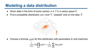
  • 47. Modeling a data distribution ● Given data in the form of some vectors in a vector space , ● Find a probability distribution over , “peaked” only on the data . ● Choose a formula for this distribution with parameters , and maximize p(x) V V pθ(x) θ 1 |T | log ∏ x∈T pθ(x) = 1 |T | ∑ x∈T log pθ(x) x ∈ T T
  • 48. Low-dimensionality of data ● Data usually lies on a low-dimensional submanifold of some high- dimensional ambient vector space. ● For example, the collection of 64 x 64 x 3 color images that are of a face live on a small sub-manifold of all possible 64 x 64 x 3 x 256 color images.
  • 49. Latent variables ● We transform to the lower-dimensional subspace of interest by writing where is a “latent variable” from the subspace. For a VAE, we assume that ● The above transformation is the sum rule for conditional probability. z pθ(x | z) ∼ normal with mean M(z) and variance Σ(z)2 p(z) ∼ standard normal pθ(x) = ∫ pθ(x | z) p(z) dz z lives in here
  • 50. The “decoder” ● The VAE “decoder” is the map . ● The formulas for and are given by neural networks. z ↦ (Mθ(z), Σθ(z)2 ) Mθ(z) Σθ(z)2 z Mθ(z)
  • 51. A difficulty ● Unfortunately, it is difficult to estimate from its integral formula. ● An easier integral would be where the distributions and are nearly identical for each . pθ(x) pθ(x) = ∫ pθ(x | z) p(z) dz ≈ 1 N N ∑ i = 0 zi ∼ p(z) pθ(x | zi) small for most , so we need a huge to estimate this. zi ∼ p(z) N pθ(x) = ∫ pθ(x | z) q(z | x) dz ≈ 1 N N ∑ i = 0 zi ∼ q(z | x) pθ(x | zi) large for most , so we don’t need large to estimate this. zi ∼ q(z | x) N q(x | z) pθ(x | z) z
  • 52. The fix ● We choose a formula for that depends on parameters . ● For a VAE, we assume that and tune the parameters so and are almost identical. ● By identical, we mean that the “KL-divergence,” a kind of measure of distance between these distributions, is small. qϕ(z | x) ∼ normal with mean μϕ(x) and variance σϕ(x)2 qϕ(z | x) pθ(z | x)ϕ q(z | x) ϕ KL(qϕ( ⋅ | x) || pθ( ⋅ | x)) := ∫ qϕ(z | x) log ( qϕ(z | x) pθ(z | x) ) dz,
  • 53. The “encoder” ● The VAE “encoder” is the map . ● The formulas for and are given by neural networks. x ↦ (μϕ(x), σϕ(x)2 ) μϕ(x) σϕ(x)2 x μ σ2
  • 54. ELBO learning objective ● In summary, we want to maximize the evidence lower bound (ELBO) loss. ● With some algebra, we can write this loss in an expected form. ● As discussed, the first term (purple) is easier to numerically estimate. ● The second term (brown) has an explicit formula which is easy to use. L(θ, ϕ) = 1 |T | ∑ x∈T [ log pθ(x) − KL(qϕ( ⋅ | x) || pθ( ⋅ | x)) ]KL(qϕ( ⋅ | x) || pθ( ⋅ | x))log pθ(x) = 1 |T | ∑ x∈T [ ∫ pθ(x | z) p(z) dz − KL(qϕ( ⋅ | x) || pθ( ⋅ | x)) ]∫ pθ(x | z) p(z) dz KL(qϕ( ⋅ | x) || pθ( ⋅ | x)) L(θ, ϕ) = 1 |T | ∑ x∈T [ ∫ pθ(x | z) qϕ(z | x) dz − KL(qϕ( ⋅ | x) || p( ⋅ )) ]∫ pθ(x | z) qϕ(z | x) dz KL(qϕ( ⋅ | x) || p( ⋅ ))
  • 55. ELBO learning objective ● The learning objective that we seek to maximize is therefore ● Compare to the previous learning objective that we sought to maximize. ● The purple and brown terms of either expression correspond. L = 1 |T | ∑ x∈T [− d(x, D(E(x)) − KL(𝒩(μϕ(x), σϕ(x)2 ) || 𝒩(0,1))] L(θ, ϕ) = 1 |T | ∑ x∈T [ ∫ pθ(x | z) qϕ(z | x) dz − KL(qϕ( ⋅ | x) || p( ⋅ )) ]∫ pθ(x | z) qϕ(z | x) dz KL(qϕ( ⋅ | x) || p( ⋅ )) −d(x, D(E(x)) −KL(𝒩(μϕ(x), σϕ(x)2 ) || 𝒩(0,1))
  • 56. Putting it all together ● Combining the encoder with the decoder gives us the VAE: Encoded Data Encoder Decoder Input Data Reconstructed Data Latent Space σ2 1 σ2 2 μ1 μ2 Diagonal Multivariate Gaussian Mean, Variance Random Sample
  • 57. References ● The original article on VAEs: https://arxiv.org/abs/1312.6114 ● Informative blogs on VAEs: ● http://gokererdogan.github.io/2017/08/15/variational-autoencoder- explained/ ● https://towardsdatascience.com/intuitively-understanding-variational- autoencoders-1bfe67eb5daf ● http://krasserm.github.io/2018/07/27/dfc-vae/ ● https://www.jeremyjordan.me/variational-autoencoders/ ● Applications of generative models in CV: https://medium.com/@jonathan_hui/gan-some-cool-applications-of- gans-4c9ecca35900
  • 58. References ● Improvements to VAEs ● PixelVAE: https://arxiv.org/abs/1611.05013 ● Perceptual loss: https://arxiv.org/abs/1610.00291 ● Different optimization criteria: https://arxiv.org/abs/1702.08658 ● VAE-GAN: https://arxiv.org/abs/1512.09300 ● Check out our VAE implementation at https://github.com/compthree/variational-autoencoder
  • 59. About Comp Three ● We are an AI and data consulting company based in San Jose. ● Our website: http://www.compthree.com ● We have resources currently available for everything from roadmaps and architecture to nuts-and-bolts front and back end ML engineering. ● Reach out to us at [email protected].