Energy aware routing for wireless sensor networks

For more Https://www.ThesisScientist.com
A Detail Comparative Routing Analysis in Wireless
Sensor Networks for Static and Mobile Environments
A Dissertation Report Submitted in the Partial Fulfillment of
The Award of the Degree of
MASTER OF TECHNOLOGY
IN
COMPUTER SCIENCE AND ENGINEERING
Under Guidance of: Submitted By:
Name of Internal Guide Name of Students
(Designation) Roll No

AODV Ad-hoc On-demand Distance Vector
CAP Contention Access Period
CBR Continuous Bit Rate
CCA Clear Channel Assessment
CFP Contention Free Period
CRC Cyclic Redundancy Check
CSMA-CA Carrier Sense Multiple Access with Collision Avoidance
CSMA-CD Carrier Sense Multiple Access with Collision Detection
CTS Clear-To-Send message
DARPA Defence Advanced Research Project Agency
DSN Distributed Sensor Networks
DSSS Direct Sequence Spread Spectrum
ED Energy Detection
FC4 Fedora Core 4
FTP File Transfer Protocol
GPS Global Positioning System
GTS Guaranteed Time Slot
GUI Graphical User Interface
IEEE Institute of Electrical and Electronics Engineers
IP Internet Protocol
IPTO Information Processing Techniques Office
ISM Industrial, Scientific and Medical
LAN Local Area Network
LQI Link Quality Indication
LR-WPAN Low Rate Wireless Personal Area Network
MAC Medium Access Control
MAN Metropolitan Area Network
MEMS Micro-Electro-Mechanical System
NAM Network Animation
NB Number of Back offs

NS Network Simulator
OTCL Object Oriented Tool Command Language
PAN Personal Area Network
PDAs Personal Digital Assistants
PHY Physical
QOS Quality of Service
RREP Route Reply
RREQ Route Request
RTS Ready-To-Send message
SSCS Service Specific Convergence Sub-layer
TCP/IP Transmission Control Protocol/Internet Protocol
UDP User Datagram Protocol
VINT Virtual Inter Network Test-bed
WLAN Wireless Local Area Network
WPAN Wireless Personal Area Network
WSN Wireless Senor Network

ABSTRACT
Deployment of sensor networks are increasing either manually or randomly to monitor
physical environments in different applications such as military, agriculture, medical
transport, industry etc. In monitoring of physical environments, the most important
application of wireless sensor network is monitoring of critical conditions. The most
important in monitoring application like critical condition is the sensing of information
during emergency state from the physical environment where the network of sensors is
deployed. In order to respond within a fraction of seconds in case of critical conditions
like explosions, fire and leaking of toxic gases, there must be a system which should be
fast enough. A big challenge to sensor networks is a fast, reliable and fault tolerant
channel during emergency conditions to sink (base station) that receives the events.
In this thesis work, firstly an attempt have been made to evaluate the performance of
DSR and OLSR routing protocol in mobile and static environments using Random
Waypoint model, and also investigate how well these selected protocols performs on
WSNs, , using OPNET 16.0 Simulation tool. The performance analysis of these protocols
will focus on the impact of the network size and the number of nodes. The performance
metrics used in this work are throughput, average end-to-end delay, network load, routing
overhead, jitter and propagation delay.
Keywords-- Ad-hoc network, OLSR, DSR, MANET, OPNET Simulation, WSN

CHAPTER 1
WIRELESS SENSOR NETWORK
In this chapter firstly introduce the basic concepts behind the emerging area of
Wireless Sensor Networks (WSN) such as, network components of Wireless Sensor
Networks, Mobility models and its standards ,at the same time we also present an
overview of the its applications and security challenges.
1.1. Introduction:
Wireless sensors network (WSN) is the collection of homogenous, self organized nodes
known as sensor nodes. These nodes have the event sensing capabilities, data processing
capabilities.

Figure 1.1 Wireless Sensor Network
The components of sensor node are integrated on a single or multiple boards, and
packaged in a few cubic inches. A wireless sensor network consists of few to thousands
of nodes which communicate through wireless channels for information sharing and
cooperative processing. A user can retrieve information of his/her interest from the
wireless sensor network by putting queries and gathering results from the base stations or
sink nodes. The base stations in wireless sensor networks behave as an interface between
users and the network. Wireless sensor networks can also be considered as a distributed
database as the sensor networks can be connected to the Internet, through which global
information sharing becomes feasible. Wireless Sensor Networks consist of number of
individual nodes that are able to interact with the environment by sensing physical
parameter or controlling the physical parameters, these nodes have to collaborate in order
to fulfil their tasks as usually, a single node is incapable of doing so and they use wireless
communication to enable this collaboration.
1.1.1 Wireless Sensor Network Model:
The major components of a typical sensor network are:
 Sensor Field: A sensor field is the area in which the all sensors nodes are placed.

Figure 1.2 : Wireless Sensor network model
 Sensor nodes: Sensor node has capabilities of event sensing, data processing and
communication capabilities.
Figure 1.3 The picture of sensor node
 Sink: A sink is a sensor node with the specific task of data receiving, data
processing and data storing from the other sensor nodes. They serve to reduce the
total number of messages that need to be sent, hence reducing the overall energy
requirements of the network. Sinks are also known as data aggregation points.
 Task Manager: The task manager also known as base station is a centralised
point of control within the network that extracts information from the network.
1.1.2 Network Components of a Wireless Sensor Node:
The main components of a general WSN are the sensor nodes, the sink (base station).
 Sensing Unit: Sensors play a very important role in wireless sensor networks by
creating a connection between physical world and computation world. Sensor is

a hardware device used to measure the change in physical condition of an area of
interest and produce response to that change. It converts the analogue data
(sensed data from an environment) to digital data and then sends it to the
microcontroller for further processing.
A typical wireless sensor node is a micro-electronic node with less than 0.5 Ah
and 1.2 V power source.
Figure 1.4: Components of a Wireless Sensor Node
 Memory Unit: Memory unit of the sensor node is used to store both the data and
program code. For data packets storing from neighbouring (other) nodes
Random Only Memory (ROM) is normally used and to storing the program
code, flash memory or Electrically Erasable Programmable Read Only Memory
(EEPRM) is used.

 Power Unit: A sensor node consist a power unit that responsible for computation
and transmission and deliver power to all its units. The basic power consumption
at node is due to computation and transmission where transmission is the most
expensive activity at sensor node in terms of power consumption. Mostly, sensor
nodes are battery operated but it can also scavenge energy from the environment
through solar cells.
 Processing Unit: Processing unit is responsible for data acquisition, processing
incoming and outgoing information, implementing and adjusting routing
information considering the performance conditions of the transmission. Sensor
node has a microcontroller which consist a processing unit, memory, converters
(analogue to digital, ATD) timer and Universal Asynchronous Receive and
Transmit (UART) interfaces to do the processing tasks.
1.1.3 WSN Communication Architecture:
The protocol stack consists of the physical layer, data link layer, network layer, transport
layer and application layer. And also consist of power management plane, mobility
management plane and task management plane. The main usage of protocol stack are
integrating data with networking protocols, communicates power efficiently through the
wireless medium. The physical layer is required for carrier frequency generation,
frequency selection, signal detection, modulation and data encryption, transmission and
receiving mechanisms. The Data Link Layer is required for medium access, error control,
multiplexing and de- multiplexing of data streams and data frame detection.
It also ensures reliable point to point and point to multi-hop connections in the network.
The MAC layer of data link layer provides the facility of collision detection and use
minimal power. The network layer is required for routing the information received from
the transport layer i.e. finding the most efficient path for the packet to travel on its way to
a destination.

Figure 1.5: Protocol Stack
The Transport Layer is needed when the sensor network intends to be accessed through
the internet. It also helps in maintaining the flow of data whenever the application
requires it. The application layer is responsible for presenting all required information to
the application and application users and propagating requests from the application layer
down to the lower layer.
1.2 Clustering in wireless sensor network:
In clustering, the sensor nodes are partitioned into different clusters. Each cluster is
managed by a node referred as cluster head (CH) and other nodes are referred as cluster
nodes. Cluster nodes do not communicate directly with the sink node. They have to pass
the collected data to the cluster head and cluster head received from data from cluster
nodes and then aggregate the data and transmits it to the base station .Thus minimizes the
energy consumption and number of messages communicated to base station. Also
number of active nodes in communication is reduced.
Sensor Node: It is the core component of wireless sensor network. It has the capability of
sensing, processing, routing, etc.

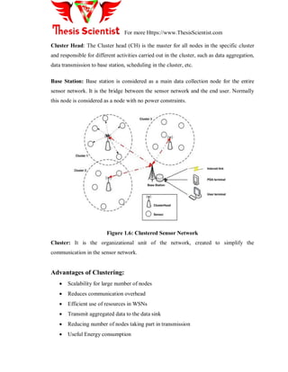
Cluster Head: The Cluster head (CH) is the master for all nodes in the specific cluster
and responsible for different activities carried out in the cluster, such as data aggregation,
data transmission to base station, scheduling in the cluster, etc.
Base Station: Base station is considered as a main data collection node for the entire
sensor network. It is the bridge between the sensor network and the end user. Normally
this node is considered as a node with no power constraints.
Figure 1.6: Clustered Sensor Network
Cluster: It is the organizational unit of the network, created to simplify the
communication in the sensor network.
Advantages of Clustering:
 Scalability for large number of nodes
 Reduces communication overhead
 Efficient use of resources in WSNs
 Transmit aggregated data to the data sink
 Reducing number of nodes taking part in transmission
 Useful Energy consumption

1.3. Characteristics of Wireless Sensor Networks
Wireless Sensor Networks have some unique characteristics. These are:
 Low power consumption: Sensor nodes are small-scale devices with volumes
approaching a cubic millimetre in the near future. Such small devices are very
limited in the amount of energy they can store or harvest from the environment.
 Ability to cope with node failures: Nodes are subject to failures due to depleted
batteries or, more generally, due to environmental influences. Limited size and
energy also typically means restricted resources (CPU performance, memory,
wireless communication bandwidth and range).
 Limited Communication Capability: The transmission range of a sensor nodes
is varied from tens of meters to hundreds of meters, which is highly depend on
the geographical environments and the natural causes. The bandwidth of a sensor
node is also very limited. Consequently, how to finish the expected tasks under
the constraint of limited communication capability is a challenge issue in
Wireless Sensor Networks.
 Limited Computing and Storage Capabilities: The computing, processing, and
storage capabilities of sensor nodes are very limited. Thus, only some basic data
processing and computing tasks can be finished on a node. Meanwhile, the
memory and storage space of sensor nodes are also very limited, where some
temporary data can be stored.
 Dynamic Network: Wireless Sensor Networks are large-scale networks. During
the working process of a Wireless Sensor Networks, some nodes may die due to
exhaust their energy or damaged by some other causes, and some new nodes may
come to join the network. Hence, how to deal with this dynamics for Wireless

Sensor Networks and make the network adapt the changes is a challenge issue
when design algorithms and protocols for Wireless Sensor Networks
 Huge Data Flows: The data produced by the sensor nodes by viewed as data
flows. Intuitively, as time goes on, huge data flows are generated by a Wireless
Sensor Networks. Among these data flows, there may be a lot of redundant data.
Considering the limitations of sensors nodes on computing, communication, and
storage capabilities, how to manage, query, analyze, and utilize these data is
another challenge works for researchers.
1.4. Applications of Wireless Sensor Networks:
Wireless sensor network can be developed for various types of application based on its
data delivery, application type and application objective. Generally WSN application can
be classified into following four classes.
1. Commercial and Industrial Applications:
a. Monitoring an Industrial Plant: The wireless sensors are used to monitor the state of
the physical plant and control device Cost savings can be achieved through inexpensive
wireless means.
b. Inventory Control: Sensor nodes are used for warehouses products tagging. This will
enable the users to track the exact location of the products as well as inventory the stock
on hand. Inserting new products can be achieved by attaching the appropriate sensor
nodes to the products. If the products are perishable, the senor node can also report the
state of the products such as days in storage or temperature.
2. Health Applications
a. Gym Workout Performance Monitoring: The gym member users pulse and
respiratory rate can be monitored via wireless sensor nodes and transmitted to a personal
computer for analysis. The gym club can monitors the exercise behaviour of members
and intervene when members need help reaching their goals.

b. Monitoring of Human Physiological Data: Sensor nodes can collected the
physiological data and stored over a period of time to study human habits and behaviour.
Sensor nodes allow greater freedom of movement and allow physicians to either monitor
an existing condition.
3. Environmental Applications:
a. Soil Condition Monitoring: Sensor nodes can monitor soil temperature and moisture
for a given area. The sensor nodes can also be fitted with a variety of chemical and
biological sensors so that the farmers can determine the level of fertilizer. This
application is most suited for vineyards as minor changes in the environment can greatly
affect the value of the crop and how it is subsequently processed.
b. Seismic Activity Detection: Sensor nodes placed in regions for detection of seismic
activity such as earthquakes, volcanic eruptions or a tsunami. Timely analysis of such
information will enable cities to be evacuated. Sensor nodes placed in regions of seismic
activity will enable geologists to monitor and predict the onset of an earthquake, volcanic
eruption or a tsunami.
4. Security and Military Applications:
A wireless sensor network can be an integral part of military command, intelligence,
surveillance, targeting systems, control, computing, and communications. They can be
quickly deployed and are fault tolerant, which makes them an ideal sensing technique for
reconnaissance and surveillance.
a. Monitoring of Force Movement and Inventory: Wireless sensor networks can be
used for monitoring of force movement and availability of equipment and
ammunition. This will enable the military commander to give order to his forces
or equipment to where it is needed most.
b. Battlefield Reconnaissance and Surveillance: A wireless sensor network can be used
to locate and identify targets for potential attacks or to support an attack by friendly

forces Deployed .And wireless sensors networks can also be used in place of guards or
sentries
2. Motivation
Recent research into wireless sensor network (WSN) has attracted great interest because
of its advantages like self identification, self diagnostics, reliability, time awareness for
co-ordination with other nodes. In WSN nodes in a network communicate with each other
via wireless communication. Moreover, the energy required to transmit a message is
about twice as great as the energy needed to receive the same message. The route of each
message destined to the base station is really crucial in terms network lifetime: e.g., using
short routes to the base station that contains nodes with depleted batteries may yield
decreased network lifetime. On the other hand, using a long route composed of many
sensor nodes can significantly increase the network delay.
But, some requirements for the routing protocols are conflicting. Always selecting the
shortest route towards the base station causes the intermediate nodes to deplete faster, this
result in a decreased network lifetime. At the same time, always choosing the shortest
path might result in lowest energy consumption and lowest network delay. Finally, the
routing objectives are tailored by the application; e.g., real-time applications require
minimal network delay, while applications performing statistical computations may
require maximized network lifetime. Hence, different routing mechanisms have been
proposed for different applications. These routing mechanisms primarily differ in terms
of routing objectives and routing techniques, where the techniques are mainly influenced
by the network characteristics.
3. Aims and objectives:
The main aim of this research study is to identify the performance challenges for selected
routing protocols in wireless sensors and then evaluate the selected routing protocols for
a selected application environment (Static and Mobile) against the set of qualitative

performance metrics for any protocol. Furthermore the another main objective of this
thesis is to identify delivery demand of the communication for the selected application, to
compare different routing protocols for these applications and to identify the protocol
suitability in the selected application environment on the basis of performance results in
order to attain efficient communication and save network resources.
The particular goals of this thesis work are to:
 Develop and design a simulation model and scenarios.
 Perform a simulation with different metrics and different scenarios.
 Analysis of the results in static and mobile environment.
 Comparative study has been done on the basis of simulation results.
 Deriving a conclusion on basis of performance evaluation.
4. Simulation Tool
In our dissertation work we are using the Optimized Network Engineering Tool (OPNET
v16.0) software for simulating selected routing protocols. OPNET is a network simulator.
Figure: Flow chart of OPNET
It provides multiple solutions for managing networks and applications e.g. network
operation, planning, research and development (R&D), network engineering and
performance management. OPNET 16.0 is designed for modelling communication

devices, technologies, and protocols and to simulate the performance of these
technologies. It allows the user to design and study the network communication devices,
protocols, individual applications and also simulate the performance of routing protocol.
It supports many wireless technologies and standards such as, IEEE 2002.11, IEEE
2002.15.1, IEEE 2002.16, IEEE 2002.20 and satellite networks. OPNET IT Guru
Academic Edition is available for free to the academic research and teaching community.
It provides a virtual network environment that models the behaviour of an entire network
including its switches, routers, servers, protocols and individual application. The main
merits of OPNET are that it is much easier to use, very user friendly graphical user
interface and provide good quality of documentation.
5. RESEARCH METHODOLOGY
Research methodology defines how the development work should be carried out in the
form of research activity. Research methodology can be understand as a tool that is used
to investigate some area, for which data is collected, analyzed and on the basis of the
analysis conclusions are drawn. There are three types of research i.e. quantitative,
qualitative and mixed approach as defined in.
5.1 Quantitative Approach
This approach is carried out by investigating the problem by means of collecting data,
experiments and simulation which gives some results, these results are analyzed and
decisions are made on their basis. This approach is used when the researchers‟ want
verify the theories they proposed, or observe the information in greater detail.
5.2 Qualitative Approach
This approach is usually involves the knowledge claims. These claims are based on a
participatory as well as / or constructive perspectives. This approach follows the
strategies such as ethnographies, phenomenology and grounded theories. When the
researcher wants to study the context or focusing on single phenomenon or concepts, they
used qualitative approach to achieve their desired goals.

5.3 Mixed Approach
Mixed approach glue together both quantitative and qualitative approaches. This
approach is followed when the researchers wants to base their knowledge claims on
matter of fact grounds. Mixed approach has the ability to produce more complete
knowledge necessary to put a theory and practice as it combined both quantitative and
qualitative approaches.
5.4 Author’s Approach
Author‟s approach towards the thesis is quantitative. This approach starts by studying the
elated literature specific to security issues in MANETs. Literature review is followed by
simulation modeling. The results are gathered and analyzed and conclusions are drawn on
the basis of the results obtained from simulation.
5.5 Research Design
The author divided the whole research thesis into four stages.
1) Problem Identification and Selection.
2) Literature study.
3) Building simulation.
4) Result analysis.

Fig. Research Methodology
1) Problem Identification and Selection
The most important phase, where it is important to select the proper problem area.
Different areas are studied with in mind about the interest of authors. Most of the time is
given to this phase to select the hot issue. The authors selected MANET as the area of
interest and within MANET the focus was given to the security issues.
2) Literature Study
Once the problem was identified the second phase is to review the state of the art. It is
important to understand the basic and expertise regarding MANETs and the security
issues involved in MANETs. Literature study is conducted to develop a solid background
for the research. Different simulation tools and their functionality are studied.
3) Building Simulation

The knowledge background developed in the literature phase is put together to develop
and build simulation. Different scenarios are developed according to the requirements of
the problems and are simulated.
4) Result Analysis
The last stage and important and most of the time is given to this stage. Results obtained
from simulation are analyzed carefully and on the basis of analysis, conclusions are
drawn.
CHAPTER2
LITERATURE REVIEW
In this chapter we have studied the various related work on Wireless Sensor
Networks (WSNs) such as its routing protocols, its application classes its and its
network simulator of Wireless Sensor Networks. By conducting literature survey,
we studied different research articles, papers including books to identify factors
which highly influence the routing protocols and affect their performance.
2.1 Related Work:

Sonam Palden.et al; (2012): In this paper authors proposed a novel energy efficient
routing protocol. The proposed protocol is hierarchical and cluster based. In this protocol,
the Base Station selects the Cluster Heads (CH). The selection procedure is carried out in
two stages. In the first stage, all candidate nodes for becoming CH are listed, based on the
parameters like relative distance of the candidate node from the Base Station, remaining
energy level, probable number of neighboring sensor nodes the candidate node can have,
and the number of times the candidate node has already become the Cluster Head. The
Cluster Head generates two schedules for the cluster members namely Sleep and TDMA
based Transmit. The data transmission inside the cluster and from the Cluster Head tothe
Base Station takes place in a multi-hop fashion. They compared the performance of the
proposed protocol with the LEACH through simulation experiments. and observation is
that the proposed protocol outperforms LEACH under all circumstances considered
during the simulation. As a future scope they state that, the protocol can be enhanced for
dealing with mobility of nodes. Even effort can be made to decide the number of clusters
dynamically and this may give better scalability to the protocol for dealing with very
large wireless sensor networks.
P. Kamalakkannan.et al; [2013]: In this paper, they proposed an enhanced algorithm
for Low Energy Adaptive Clustering Hierarchy–Mobile (LEACH-M)protocol called
ECBR-MWSN which is Enhanced Cluster Based Routing Protocol for Mobile Nodes in
Wireless Sensor Network. ECBR-MWSN protocol selects the CHs using the parameters
of highest residual energy, lowest Mobility and least Distance from the Base Station. The
Base Station periodically runs the proposed algorithm to select new CHs after a certain
period of time. It is aimed to prolonging the lifetime of the sensor networks by balancing
the energy consumption of the nodes. The experiments were performed to evaluate the
performance of the proposed protocol in terms of four factors like Average Energy
Consumption, Packet Delivery Ratio, Throughput, Routing Overhead and Average end to
end Delay. The simulations results indicates that the proposed clustering approach is
more energy efficient and hence effective in prolonging the network life time compared
to LEACH-M and LEACH-ME. They also suggest in future scope that the algorithms and
techniques implemented in the proposed protocol will be optimized in order to minimize

energy and routing related packets, which in turn lead to reduced routing overhead. Then
to find the energy consumption while delivery of packets under non-uniform transmission
situations. And also the proposed protocol will improve the performance to decrease the
delay. Particularly for reaching the optimal solution for mobile sensor networks is an
open issue.
Pallavi Jindal. et al; (2013):In this paper authors shows the various routing techniques
like LEACH, WLEACH, LEACH-CC, GAF, CODE. They show the comparison between
LEACH, WLEACH and LEACH-CC. Their survey shows the limitation of basic leach.
Leach use TDMA or CDMA Mac to share channel. The goal of LEACH is to lower the
energy consumption required to create and maintain clusters in order to improve the life
time of a wireless sensor network. LEACH is a hierarchical protocol in which most nodes
transmit to cluster heads, and the cluster heads aggregate and compress the data and
forward it to the base station (sink). Each node uses a stochastic algorithm at each round
to determine whether it will become a cluster head in this round. LEACH assumes that
each node has a radio powerful enough to directly reach the base station or the nearest
cluster head, but that using this radio at full power all the time would waste energy. By
data-fusion and energy-equilibrium, LEACH can extend the life of network .But there are
some disadvantage of leach that are: first it uses random number to decide a node
whether becomes a cluster-head node, so when a low-energy node becomes cluster-head
node, it will die immediately. Secondly, LEACH doesn‟t care the neighbor nodes when
makes cluster head nodes, so when some nodes are far from its cluster-head node in long
time, they will die immediately too. Finally, every node uses single-jump routing to
transmit data, which makes that commutation between nodes too costly.
L.I. Jian. et al; (2013):in their paper they aim at the node characteristic of uneven
distribution in the real environment the improved algorithm combines the advantages of
EUUC algorithm and PEGASIS algorithm. The new improved algorithm improves
uneven energy consumption of the cluster head nodes under EUUC algorithm, also
reduces the complexity of clustering signaling, as well as takes real-time problems into
consideration. By calculating dispersion coefficient of the cluster to determine the
communication topology within each cluster and by using multi-objective particle swarm

optimization to optimize cluster head routing. The simulation results of the algorithm
shows that the improved algorithm is more suitable for large-scale wireless sensor
networks, and makes overall network performance more effective. But improved
algorithm is to measure distance based on the signal intensity. In real application, the
signal intensity is to being effected by outside environment.
R. Balasubramaniyan et al; (2013):In the paper authors consider the study that in
WMASNs, the number of control packets for flooding increases exponentially with the
number of nodes. The CBRP (Cluster-Based Routing Protocol)methods were proposed to
solve the problem of exponential increase. The CBRP methods have been widely used to
achieve efficient management and extension of distributed nodes. Well-known CBRP
methods include LCA (Linked Clustered Algorithm), LID (Lowest-ID), LCC (Least
Cluster Change),MCC (Maximum Connectivity) and RCC (Random Competition
Clustering) . These existing algorithms have clustering criteria for selecting cluster heads
and are based on the minimum cluster overlap method in the formation of clusters. These
algorithms, however, cannot guarantee stability due to the ambiguity in the selection of
cluster heads. Thus, several clustering algorithms were proposed in WMASNs to improve
performance and reduce overhead. Selecting the cluster head is based on the mobility of
nodes in, and on the mobility of nodes and power capacity in. These algorithms have the
advantage of clear selection of the cluster head, but they have the problem of requiring
correct information for the attributes and relationships of nodes. Though many clustering
algorithms are proposed, few algorithms are dedicated for wireless mobile ad hoc
networks.
Ali Norouzi.et al;(2013): In this paper authors made an elaborate study on the routing
method featured with optimum energy consumption in wireless sensor networks. Some of
routing protocols with high energy efficiency (LEACH, Director Diffusion, Gossiping,
PEGASIS, and EESR) were examined. Authors have also view the strategies of the
protocol for WSNs such as data aggregation and clustering, routing, different node role
assignments, and data-center methods. The routing protocols were compared regarding
variety of metrics influencing requirements of the specific application .The result of their

paper in which the comparison showed that Gossiping consumes a medium amount of
energy and best performance was obtained by PEGASIS and LEACH.
Franscisco j. Martinez et al; (2009): In this paper authors present a survey and
comparative study of several publicly available network simulators, mobility generators
and Wireless sensor networks simulators. In their work , the network simulators like NS-
2, SNS, GloMoSim, SWANS, and QualNet briefly described by authors. In this paper
authors also present comparative study of various mobility generator like SUMO, MOVE
FreeSim, CityMob, STRAW, and Netstream. In their work authors conclude that SUMO,
STRAW and MOVE have good traffic model support and also have some good features
but these are the best. Finally the authors present briefly introduction of Wireless sensor
networks simulators such as Trans, MobiREAL, GrooveNet, NCTUns. According to the
authors survey GrooveNet and NCTUns are more frequently used for Wireless sensor
networks simulations than simulation tools.
Bhardwaj P. K et al; (2012): In this paper authors analyze performance of two routing
protocols AODV and OLSR by using OPNET Modelar 14.5.In their work ,authors create
a network scenario of 50 nodes with the comparison of network load media access delay
and throughput to examine the AODV and OLSR routing protocols with simulation
parameters like 800*800 m campus area , 50 nodes and 20 minutes simulation time
.According to the authors simulation result OLSR routing protocol shows low media
access delay and low network load in comparison of AODV , with the overall
performance OLSR is better than AODV but it is not necessary that OLSR is always
better than AODV.
Moravejosharieh A. et al; (2013):Here authors, reveals the performance analysis of
reactive routing protocols AODV, AOMDV and DSR. In their work, authors performed
comparison with proactive routing protocol DSDV. In this paper authors used NS-2.34
simulation tool for simulation purpose with taken various parameters such as 200 second
simulation time , 10*1000 m simulation area and 100 bytes packet size, by using
performance metrics such as packet delivery ratio, average packet loss ratio and average
end to end delay of packets are investigated on the basis of node velocity and node
density .

According to the authors simulation result, DSDV routing protocol shows the worst
packet delivery ratio and AOMDV and AODV have highest average end to end delays.
Siva D. Muruganathan. et al; (2010):here authors have made a comparison between the
average query response time of the Two-level Hierarchical Clustering based Hybrid-
routing Protocol (THCHP) and Adaptive Periodic Threshold-sensitive Energy Efficient
sensor Network (APTEEN)Protocol, and the result shows that THCHP is better suited
than APTEEN for delay sensitive WSN applications such as forest fire detection.
APTEEN utilizes adaptive threshold values and a periodic update interval parameter to
switch between proactive and reactive modes of data routing where as THCHP, an
alternative hybrid routing protocol.
Waghmare et al; (2008):in this paper authors try to make best use of GRPC channels by
proposing a cluster based multi channel communication scheme. In this scheme authors
assumed that each sensors node is equipped with two GRPC transceiver that can work on
two different channel simultaneously. In their work they divide time in to periods that can
be repeated every T millisecond. And each period is further divide into sub periods for
exchange data.
Mahmud et al; (2008):Here, authors proposed a hybrid media access technique for
cluster based wireless sensors networks ,this technique is based on the scheduled based
approach such as TDMA for intra cluster based communications and management , and
contention based approach for the inter cluster based communications and management.
In this scheme authors used a control channel for delivering the safety and non safety
application related messages to the nearby clusters.
Wan-Li Zhao. et al;(2010): in this paper authors have discussed the routing algorithm
like Leach a clustering routing protocol which was first proposed in wireless sensor
networks. Cluster head in LEACH can be randomly selected to average the power
consumption in the whole network, yet the cluster head selection ignores such indicators
as the residual energy of the nodes and the number of neighboring nodes. As a result, a
node tends to act as a cluster head node for too long before it gets ineffective or there is
no cluster head node to manage an area for a long time with slim chances of data
collection. Even worse, from the perspective of the whole network, cluster heads are not

optimized. Secondly, in HEED algorithm there are two parameters as the main references
in cluster head selection. The major parameter depending on the residual energy of the
node is used to randomly select the set of the initial cluster headed nodes. The node with
more residual energy will be a cluster head in large probability.
Paul J.M. Havinga. et al; (2013): in this paper authors made the study of basic
clustering algorithm Leach. A comparison is made between Leach and Leach. In this
paper they propose REC+, a Reliable and Energy-efficient Chain-cluster based routing
protocol, which aims to achieve the maximum reliability in a multi-hop network by
finding the best place for the Cluster Head (CH) and the proper shape/size of the clusters
without the need of using any error controlling approaches that can be quite expensive in
terms of computation and communication overhead. Most importantly, REC+ relaxes
some strong assumptions that other cluster-based routing algorithms rely on, which make
them inapplicable for real WSNs. Simulation results show that REC+ outperforms a
number of other approaches in terms of delay, energy, delay*energy and lifetime.
Compared with existing approaches that reform clusters in each round, REC+ starts to
change the clusters hopes when the energy goes below a threshold or end to end
reliability changes significantly. In the ongoing work, authors will work on making this
centralized cluster-chain routing approach autonomous and distributed.
Akyildiz.I.F. et al;(2002):In this paper authors present a communication architecture for
wireless sensor networks and proceed to survey the current research pertaining to all
layers of the protocol stack: Physical, Data Link, Network, Transport and Application
layers. A wireless sensor network is deal as being composed of a large number of nodes
which are deployed dense lyin close proximity to the phenomenon to be monitored. Each
of these nodes collects data and its purpose is to route this information back to a sink. The
network must possess self-organizing capabilities since the positions of individual nodes
are not predetermined. The authors point out that none of the studies surveyed has a fully
integrated view of all the factors driving the design of sensor networks and proceeds to
present its own communication architecture and design factors to be used as a guideline
and as a tool to compare various protocols.

2.2 Classification of Routing protocols in WSN:
Routing protocol of WSN can be categorized according to the nature of wireless sensor
network and its architecture. Wireless sensors network can be classified in to two broad
categories, network architecture based routing protocols and route selection based routing
protocols.
2.2.1 Architecture Based Routing Protocols:
In the WSN routing protocols can also divided according to the structure of network.
Protocols included into this category are further divided into three subcategories
according to their functionalities. These protocols are:
 Flat-based routing
 Hierarchical-based routing
 Location-based routing
2.2.2 Route Selection Based Routing Protocols:
This classification of protocol is based on how the source node finds a route to a
destination node and can be further classified in to two categories.
Proactive Routing Protocols: These types of protocols are table based because they
maintain table of connected nodes to transmit data from one node to another and each
node share its table with another node.
Reactive Routing Protocols: These type of routing protocols is also known as On
Demand routing protocols because it establish a route from source to destination
whenever a node has something to send thus reducing burden on network.
2.3Route Selection Base Classification of Routing Protocols:
This classification of protocol is based on how the source node finds a route to a
destination node and can be further classified in to two categories.
2.3.1: Proactive Routing Protocols:

Figure 2.1: Proactive routing protocols routing scheme
These types of protocols are table based because they maintain table of connected nodes
to transmit data from one node to another and each node share its table with another
node. Different types of proactive routing protocols are Destination Sequence Distance
Vector Routing (DSDV), Optimized link state routing (OLSR) and Fisheye State
Routing.
Ad hoc On Demand Distance Vector (AODV):
Ad hoc On Demand Distance Vector(AODV)is an pure reactive routing protocol which is
capable of both unicasting and multicasting. In Ad hoc On Demand Distance Vector
(AODV), like all reactive protocols, it works on demand basis when it is required by the
nodes within the network. When source node has to send some data to destination node
then initially it propagates Route Request (RREQ) message which is forwarded by
intermediate nodes until destination is reached. A route reply message is unicasted back
to the source node if the receiver is either the node using the requested address, or it has a
valid route to the requested address that is shown is figure 2.10.

(a) (b)
Figure 2.2: AODV route discovery process. (a) Propagation of the RREQ. (b) Path
of the RREP to the source.
Working of Ad Hoc On Demand Distance Vector Routing (AODV):
The Ad hoc On-Demand Distance Vector (AODV) allows the communication between
two nodes via intermediated nodes, if those two nodes are not within the range of each
other. To establish a route between source to the destination, AODV using route
discovery phase, along which Route Request message (RREQ) messages are broadcasted
to all its neighboring nodes. This phase makes sure that these routes do not forms any
loops and find only the shortest possible route to the destination node. It also uses
destination sequence number for each route entry, that ensures the loop free route, this is
the one of the main benefit of AODV routing protocol. For example if two different
sources sends two different request to a same destination node, then a requesting node
selects the one with greatest sequence number. In the route discovery phase several
control messages are defined in AODV. Different control messages are defined as
follows.
RREQ (Route Request):

When any node wants to communicate with other node then it broadcast route request
message (RREQ) to its neighboring nodes. This message is forwarded by all intermediate
nodes until destination is reached. The route request messages (RREQ) contains the some
information such as RREQ id or broadcast id, source and destination IP address, source
and destination sequence number and a counter.
RREP (Route Reply):
When any intermediate nodes received Route Request (RREQ) message then it unicast
the route reply message (RREP) to source node either it is valid destination or it has path
to destination and reverse path is constructed between source and destination. Each route
reply message (RREP) packet consist of some information such as hop count, destination
sequence number, source and destination IP address.
RERR (Route Error):
Whenever there is any link failure arises in the routing process then route error message
(RERR) is used for link failure notifications. The route error message RERR) consist of
some information such as Unreachable Destination node IP Address, Unreachable
Destination node Sequence Number.
AODV Route Discovery phase:
To establish a route between source node to the destination node, AODV using route
discovery phase, along which the Route Request message (RREQ) messages are
broadcasted to all its neighbouring nodes. This phase makes sure that these routes do not
forms any loops and find only the shortest possible path to the destination node. It also
uses destination sequence number for each route entry, that ensures the loop free route,
this is the one of the main benefit of AODV routing protocol.
For example if two different sources sends two different request to a same destination
node, then a destination node selects only that node having largest sequence number. In
the route discovery phase several control messages are defined in AODV protocol.
Different control messages are defined as follows.

AODV Route Table Management:
In AODV, Routing table management is required to avoid those entities of nodes that do
not exist or having invalid route from source to destination. The need for routing table
management is important to make communication loop free. It consists of following
characteristics to maintain the route table for each node
•Destination IP address
• Total number of hops to the destination
• Destination sequence numbers
• Number of active neighbors
• Route expiration time
AODV Route Maintenance:
In AODV ,when any node in the network detects that a route is not valid anymore for
communication it delete all the related entries from the routing table .And it sends the
Route reply message(RREP) to all current active neighboring nodes to inform that the
route is not valid anymore for communication purpose.
2.3.2: Reactive Routing Protocols:
These type of routing protocols is also known as On Demand routing protocols because it
establish a route from source to destination whenever a node has something to send thus
reducing burden on network. Reactive routing have route discovery phase where network
is flooded in search of destination that shown in figure 2.3. There are different types of
Reactive routing protocols like AODV, DSR, TORA.

Figure 2.3 Reactive routing protocols routing scheme .

Chapter 3
Simulation Environment
3.1 Software Environment
In our dissertation work we are using the Optimized Network Engineering Tool (OPNET
v14.5) software for simulating selected routing protocols. OPNET is a network simulator.
It provides multiple solutions for managing networks and applications e.g. network
operation, planning, research and development (R&D), network engineering and
performance management. OPNET 14.5 is designed for modelling communication
devices, technologies, and protocols and to simulate the performance of these
technologies. It allows the user to design and study the network communication devices,
protocols, individual applications and also simulate the performance of routing protocol.
It supports many wireless technologies and standards such as, IEEE 802.11, IEEE
802.15.1, IEEE 802.16, IEEE 802.20 and satellite networks. OPNET IT Guru Academic
Edition is available for free to the academic research and teaching community.
Figure 3.1: Flow chart of OPNET

It provides a virtual network environment that models the behaviour of an entire network
including its switches, routers, servers, protocols and individual application. The main
merits of OPNET are that it is much easier to use, very user friendly graphical user
interface and provide good quality of documentation. The OPNET usability can be
divided into four main steps. The OPNET first step is the modelling, it means to create
network model. The sec step is to choose and select statistics. Third step is to simulate the
network. Fourth and last step is to view and analyze results.
3.2 Simulation results and Statistics
In OPNET there are two kinds of statistics, one is Object statistics and the other is Global
statistics. Object statistics can be defined as the statistics that can be collected from the
individual nodes. On the other hand Global statistics can be collected from the entire
network. When someone choose the desired statistics then run the simulation to record
the statistics.
Table 1. Simulation Parameters
Simulation Parameters
Examined Protocols OLSR and DSR
Number of Nodes 100,150,200, 250 and 300
Types of Nodes Static
Simulation Area 50*50 KM
Simulation Time 1800 seconds
Pause Time 200 s
Performance Parameters Throughput, Delay, Network load
Traffic type FTP
Mobility model used Random waypoint
Data Type Constant Bit Rate (CBR)
Packet Size 512 bytes
Trajectory VECTOR
Long Retry Limit 4
Max Receive Lifetime 0.5 seconds
Buffer Size(bits) 25600
Physical Characteristics IEEE 802.11g (OFDM)

Data Rates(bps) 54 Mbps
Transmit Power 0.005
RTS Threshold 1024
Packet-Reception Threshold -95
These collected results are viewed and analyzed. To view the results right click in the
project editor workspace and choose view results or click on DES, results then view
results.
3.3 Simulation Environment
The dissertation work is carried out in the OPNET Modeler 16.0. Below in fig. it is
showing the simulation environment of one scenario having 200 mobile nodes for DSR
routing protocol. The key parameters are provided here i.e. delay, network load and
throughput. We run eight scenarios. In every scenario there are different numbers of
mobile nodes and different mobility. In first scenario we have 100 mobile nodes for
simulating OLSR routing protocol. In second scenario we have 100 mobile nodes for
simulating DSR routing protocol and so on that shown in table.
Table 2 Scenario used
Scenarios Nodes and Its Types Protocol
Scenario 1 100 Static Nodes OLSR
Scenario 2 100 Static Nodes DSR
Scenario 1 100 Mobile Nodes OLSR
Scenario 2 100 Mobile Nodes DSR

Each scenario was run for 12000 second (simulation time). All the simulations show the
required results. Under each simulation we check the behaviour of OLSR and DSR. Main
goal of our simulation was to model the behaviour of the routing protocols. We collected
DES (global discrete event statistics) on each protocol and Wireless LAN. We examined
average statistics of the delay, network load and throughput for the MANET. A campus
network was modelled within an area of 2000 m x 2000 m. The mobile nodes were
spread within the area. We take the FTP traffic to analyze the effects on routing
protocols. We configured the profile with FTP application. The nodes were wireless LAN
mobile nodes with data rate of 11Mbps.
3.3 Performance Parameters
Here are different kinds of parameters for the performance evaluation of the routing
protocols. These have different behaviours of the overall network performance. We will
evaluate three parameters for the comparison of our study on the overall network
performance. These parameters are delay, network load, and throughput for protocols
evaluation. These parameters are important in the consideration of evaluation of the
routing protocols in a communication network. These protocols need to be checked
against certain parameters for their performance. To check protocol effectiveness in
finding a route towards destination, we will look to the source that how much control
messages it sends. It gives the routing protocol internal algorithm‟s efficiency. If the
routing protocol gives much end to end delay so probably this routing protocol is not
efficient as compare to the protocol which gives low end to end delay. Similarly a routing
protocol offering low network load is called efficient routing protocol [17]. The same is
the case with the throughput as it represents the successful deliveries of packets in time.
If a protocol shows high throughput so it is the efficient and best protocol than the routing
protocol which have low throughput. These parameters have great influence in the
selection of an efficient routing protocol in any communication network.
3.3.1 Delay
The packet end-to-end delay is the time of generation of a packet by the source up to the
destination reception. So this is the time that a packet takes to go across the network. This

time is expressed in sec. Hence all the delays in the network are called packet end-to-end
delay, like buffer queues and transmission time. Sometimes this delay can be called as
latency; it has the same meaning as delay. Some applications are sensitive to packet delay
such as voice is a delay sensitive application. So the voice requires a low average delay in
the network. The FTP is tolerant to a certain level of delays. There are different kinds of
activities because of which network delay is increased. Packet end-to-end delay is a
measure of how sound a routing protocol adapts to the various constraints in the network
to give reliability in the routing protocol. We have several kinds of delays which are
processing delay (PD), queuing delay (QD), transmission delay (TD) and propagation
delay (PD). The queuing delay (QD) is not included, as the network delay has no concern
with it [16].
3.3.2 Network Load
Network load represents the total load in bit/sec submitted to wireless LAN layers by all
higher layers in all WLAN nodes of the network. When there is more traffic coming on
the network, and it is difficult for the network to handle all this traffic so it is called the
network load. The efficient network can easily cope with large traffic coming in, and to
make a best network, many techniques have been introduced.
High network load affects the MANET routing packets and slow down the delivery of
packets for reaching to the channel , and it results in increasing the collisions of these
control packets. Thus, routing packets may be slow to stabilize. Network load is shown in
the below figure 4.6.
3.3.3 Throughput
Throughput is defined as; the ratio of the total data reaches a receiver from the sender.
The time it takes by the receiver to receive the last message is called as throughput.
Throughput is expressed as bytes or bits per sec (byte/sec or bit/sec). Some factors affect
the throughput as; if there are many topology changes in the network, unreliable
communication between nodes, limited bandwidth available and limited energy. A high
throughput is absolute choice in every network.

IMPLEMENTATION PROCEDURE:
To implement the AODV and DSR routing protocols in Vehicular ad hoc network we
have to go through the following number of steps.
A. Define Initial Simulation Parameters
1. Choose Campus network of size 1500 m x 1500 m (simulation area) and click on
next that shown in figure A.1 and then select MANET and click YES.
Figure A.1: Defining simulation area
2. From MANET object palette drag and drop the one wlan_server (fixed node) onto
the project editor workspace.

Figure A.2: Simulation setup
3. From MANET object palette drag and drop the several wlan_wkstn (mobile
nodes) onto the project editor workspace according to the Table 4.2.

4. Click Edit  select all in subnet  select edit attributes
5. Click Protocol  IP  Addressing  Auto-assign IPv4 addresses
6. Right click and go to Edit attributes and then expand AD HOC Protocols and
choose the appropriate protocol that shown in figure A.3.
Figure A.3: Defining Ad hoc protocols
7. For apply appropriate protocol on selected object tick on „apply to selected
objects‟  click OK  Save
B. Application Configuration

This procedure defines the configuration steps for setting up the application that will be
deployed in the profile configuration.
1. Drag and drop the application configuration object from the MANET object
palette onto the project editor workspace and name it appropriately
2. Right click and go to edit attributes
3. Expand application definitions and enter the number of rows (1)
4. Click on the row and enter the name (FTP)
5.
Figure A.4: Application Configuration
6. Under description choose Ftp, High load and click OK. This sets the application
to model the high load FTP traffic.

C. Profile Configuration
This procedure defines the configuration of the profiles to be deployed in the MANET.
1. Drag and drop the Profile Configuration object from the MANET object palette
onto the project editor workspace and name it appropriately
2. Right click and go to edit attributes
3. Expand profile configuration and enter the number of rows (1)
4. Enter the profile name
5. Under applications enter the number of rows (1) and choose FTP
6. Under FTP set the start time offset (seconds) to constant (0) and duration
(seconds) to constant (10). This sets the time from the start of the profile to the
start of the application.

7. Under FTP repeatability set inter-repetition time (seconds) to uniform (10, 20)
and number of repetitions to constant (3). This defines when the next session of
the application will start and the distribution name and parameters used for
generating random session counts respectively.
8. Set the start time (seconds) to uniform (100, 3400) and duration to end of
simulation. This defines at what instance the profile will start from the beginning
of the simulation.
9. Leave repeatability at default of constant (300) for inter-repetition time and
constant (0) for number of repetitions.
10. Click OK
D. Deploying Traffic
To deploy the configured profile to the network, follow the following procedure.
1. Protocol  Applications Deploy Defined
2. Select all mobile nodes and transfer to sources under your profile
3. Select the server and transfer to server under application: FTP
4. Click apply and then OK to complete the deployment

Figure A.6: Deploying Traffic
E. Mobility Configuration
Mobility Configuration defines the mobility pattern and model that the nodes will follow
during the simulation. We use the random waypoint mobility model for our simulations.
1. Drag and drop the mobility configuration object from the object palette onto the
workspace and name it appropriately
2. Right click on the mobility configuration object and edit attributes that shown in
figure A.7.
3. In mobility configuration object attribute dialog box firstly expand default random
waypoint then under the random waypoint parameters set speed (meters/seconds)
to constant (10). This sets the speed at which the mobile node will be moving.
4. Under the random waypoint parameters set pause time (seconds) to constant
(200). This sets the duration of the pause time for the mobile stations before
changing direction to the new destination during the simulation and start time
(seconds) to constant (0).
5. Leave the rest as default and click OK
6. To deploy the mobility profile to the MANET, Select Topology  Random
Mobility  Set mobility profile
7. Enter the default random waypoint profile and click OK

Figure: Mobility configuration
F. Collect Statistics
The following procedure should be followed to collect global statistics for all the nodes.
1. In the workspace, right click and choose “choose individual DES statistics”
2. Expand global statistics and choose AODV, DSR and wireless LAN
3. Click OK and save
G. Duplicate Scenario
1. Scenarios  Duplicate scenarios
2. Enter the name of the new scenario
3. Change the number of mobile nodes, AD HOC protocol and speed as appropriate
according to the table above
4. Save.
5. Repeat the procedure for all the protocols in each category.

H. Running Simulation
1. For running scenarios firstly we click on Scenarios  Manage Scenarios. After
that Manage Scenarios window will pops up, in this window we will enter the
appropriate simulation time of all defined scenarios.
2. In Manage Scenario window, click „collect‟ under results for all the scenarios and
enter the appropriate simulation time for all scenarios then click OK to run the
simulation. After that DES Execution Manager window will be appear that shown
in figure A.8.
Figure A.8: DES Execution Manager
I. Viewing Results
1. For viewing result firstly we click on DES  Results  Compare Results or
View Result.
2. Select the scenarios or project from the Result Browser pop up window for which
you want to compare the results.

Figure A.10: Result Browser
3. In result browser Expand Global statistics, choose the appropriate statistics you
want to view that shown in figure A.10.

Chapter 5
Results and Analysis
This chapter presents and analyzed the results of DSR and OLSR simulations. We have
presented our results according to the scenarios we choose in two networks having static
and mobile nodes. Fixed node network represents data gathering applications in WSN
while mobile nodes depicts object tracking applications.
5.1. Fixed Nodes Scenarios for DSR and OLSR
In a fixed node network first scenario we increased the number of fixed nodes to check
protocols behavior with changing network size by looking at WLAN metrics and routing
overhead. . All participating nodes in both scenarios were considered as fixed and
submitting nodes, communicating to sink node within a regular interval. The application
used for all scenarios was FTP with packet size 512 bytes with packet rate of 4
packet/sec. Each scenario was simulated for 3600 seconds. 100 fixed nodes were used
initially and results were collected with and without node failure. Then nodes were
increased up to 250 and after simulation results were collected for end to end delay,
throughput and network load. In each scenario two different protocols DSR and OLSR
were implemented (simulated) in order to evaluate their performance for designed
network in the presence of scalability and node failure. The input parameters used for
both scenarios were used the same show in table 1 except number of nodes. The results
for each metric are show in graph below with respect to scenarios.
5.1.1 Network Load
In figure 5.1-5.4, the graphs represent the network load in bits per second, wherein the
horizontal line shows the simulation time in seconds and the vertical line indicates the
network load in bits per second. To find routes, routing protocols used to send control
information (packets). These control information along includes basically route request

sent, route reply send and route error sent packets. Routing In order to check the protocol
effectiveness in finding routes towards destination, it is interesting to check how much
control packets it sends. This metric used to measure the internal algorithm‟s efficiency
of routing protocol. The larger is routing overhead of a protocols (in packets/ bytes),
larger will be the wastage of the resources (bandwidth). Therefore, it is necessary to
examine the routing overhead of a protocol in order to determine its efficiency.
Considering the results in figure 5.1, we observed the behavior of DSR in 100 nodes case
without node failure scenario that DSR generates considerable routing overhead as
simulation starts but then after a specific time interval it decreases overhead which
indicates the routes establishment after which the overhead decrease regularly. Besides,
DSR seems to generate more overhead if network grows as it use source routing therefore
if a routes is not available from a node to destination somewhere in the middle it will
propagate SOURCE REQUEST in the network. This can also lead to the generation of
REQUEST ERRORS messages causing also routing overhead. While in small network of
100 nodes it performs better with negligible routing overhead which is discussed later.
Furthermore, we found a notable change in DSR behavior in 150 nodes network case
with nodes failure scenario shown in Figure 5.2 It gives the routing overhead of
1packet/sec in 100 nodes case when it application runs but then quickly drops its
overhead ration to 125bits/sec and stay with this ratio for rest of the simulation time. This
implies that for small network DSR outperforms and makes it better choice for routing
due to its reactive nature. This means that it sends control messages to nodes only when it
is required and do not creates any overhead by sending periodic updates or by maintain
routes information. On other hand, in 0 nodes scenario it jumps and gives 7100 bits/sec of
routing overhead. A minor drop after I minute can be seen and then again it rises to 7400
bits/sec and stay for about 2 minutes with this rate. Similarly, again a minor rise is clear
for the next minute but then a sudden drop up to 4800 bits/sec. the routing overhead rate
then further decreasing the same way and shows a slight small rise again at the end of
simulation. So this behavior of DSR in 150 nodes case in node failure scenario shows its
operation nature very clearly. As it is clear from the graph that it‟s routing overhead a
smaller than that of without node failure scenario but it treats both the failed and working

nodes in the same way. This is because of source routing nature of DSR. As there is
neither routing table information nor link status information (hello messages) present to
DSR, therefore it starts by sending a large amount of control messages (ROUTE
REQUESTS) to different nodes to reach a destination when application just starts running
which is shown in the start of simulation. But here we can see the difference in behavior
with respect of scenario without node failure. As its overhead does not drop directly in
start which means ROUTE REPLIES did not received and ROUTE ERROR generated to
source which increase the overhead further. While the direct drop shows the successful
route finding via same or different path and reduces overhead. On the other hand, if we
look at behavior of OLSR it gives a consistent nature of routing overhead due to its
proactive routing nature. This means that path to all nodes are already defined and
calculated. The only overhead created at network is the periodic updates of routing
information which is slightly low. Although network size will affect the routing overhead
but it remains stable and consistent.
Figure 5.1: Network load of OLSR and DSR for 100 Static nodes.

Figure 5.4: Network load of OLSR and DSR for 250 Static nodes

5.1.2 End-to-End Delay
During the transmission, submitting nodes (sender) in WLAN sends data (packet) to the
recipient nodes which receive this data at its MAC layer and then forwarded to higher
layers. By end-to-end delay, we mean the end-to-end delay of the entire packet received
at WLAN MAC of all nodes in the network and forwarded to higher layer. This includes
medium access delay at source MAC, individual reception of all fragments and frames
transmission of frames through access point delay if enabled. In figure 5.5, we can see the
behavior of DSR and OLSR for both 100 and 150 fixed nodes scenario with and without
random node failure. If we look at the scenario without node failure, it is clear from the
figure that, OLSR gives the lowest and consistent delay as compare to DSR in both small
and large network. As the application starts it shows a minor spike but then it stay
constant for the rest of the simulation time. OLSR is the proactive protocol which means
that whenever application layer is interested to transmit traffic, routes in a network are
always available. Periodic nature of routing updates provides fresh route to use. The use
of predefined and pre-computed routes towards every node results in consistent nature of
delay. OLSR use two types of control messages i.e. Hello and topology control messages.
To find information about link status and host‟s neighbor it use hello message which only
sent to one hop away. And to share own advertized neighbors, it broadcast topology
control messages periodically. Now, If we look at graph of 100 and 150 nodes without
node failure in Figure 5.6, it can be seen that it show a minor spick when the application
starts running and then directly comes to a constant state throughout the entire simulation
duration. This spike is show in time window between 0.0003 and 0005 seconds and then
it‟s consistent behavior in term of delay is show by its value on staying at 0.0004 sec. The
reason behind its initial spick (which in negligible) is its initial hello messaging use to
share the link status and host‟s neighbor information. After sharing this information, due
to its proactive nature path toward every node is always ready so it gives lowest and
consistent delay. This means that, the absence of route discovery mechanism (Pre-
computed) in OLSR ensures minimum latency.

Figure 5.5: End to End Delay of OLSR and DSR for 100 Static nodes

5.3 Throughput
The results of throughput are shown in figure 5.9-5.12. Throughput is the ratio of total
amounts of data that reaches at the receiver end in the given period of time. The X-axis
represents the time in second and Y-Axis indicates the throughput in bits per second.
When the number of node increases, the throughput will also increase and hence the
performance will be high.
The ratio of total data received by a receiver from a sender for a time the last packet
received by receiver measures in bit/sec and byte/sec This means that if high throughput
is to be achieved, network delay should be low. The behavior of both routing protocols
both in presence and absence of node failure for a WLAN consisting 100 & 150 is shown
in figure 2 below. By looking at figure below we can see the overall throughput at
WLAN reduced approximately up to 50% in presence of node failure with respect to
without node failure scenario. This indicates that if nodes will fail in a network, the
overall number of transmitting data (bits/bytes/packets) will decreased accordingly
because of the less number of active flow at particular time (simulation time). As we are
interested in protocols behavior so we will look at each protocol in both scenarios to
compare their performances. In without node failure scenario we can see that, in 100
nodes network DSR throughput rate starts with approx 4000 bit/sec and within no time it
decreases up to 49000 bit/sec. the fact is, since DSR operates using source routing which
means it construct source route in packet‟s header by giving the addresses of all nodes the
packet has to be forwarded in order to reach the destination. This implies that it does not
have any routing table information except source cache, therefore for each node it has to
discover a route which involves route discovery, route reply packet and also need route
maintenance at each hop. This causes a significant delay before data transmission also
increase routing overhead. So it is clear from the graph that it performs worst as
compared to OLSR and cannot maintain its rate at which it started. The reason here is the
increasing number of nodes for which it has to establish routes. The more will be the
number of nodes the more will be degradation in its performance due to the reason of

delay at each hop which can be seen in DSR 100 nodes case in the same graph. It is also
clear that in small network case (100 nodes), although its throughput rate is effected
approx by 50% but then quickly for the rest of simulation time it maintain its
transmission rata slightly consistent. While in 100 nodes case, its rate not only decreased
to half of its rate at starting time but also it took longer time to maintain its rate slightly
stable. This indicates that, if the number of nodes will increased the more time it will take
for routing to reach all nodes and route maintenance as well . While looking at node
failure scenario for both 100 & 150 nodes, it depicts that the performance of DSR drops
from 50,000 bit/sec to 20,000bit/sec and in 100 nodes scenario it drops slightly with
greater ratio i.e. from 100,000 bits/sec to 40,000. This again implies that the presence of
random node failure will affect dense populated network badly as compare to small
network. The reason is, in a large network it becomes difficult to discover a route from
source to destination with the presence of failed node both by resources consumption
(memory, energy) and overhead complexities. Looking at OLSR performance in 100 &
150 nodes scenarios without node failure, it not only out performs but maintains its rate
stable after a short spike in both cases. This spike is because of control messages it needs
to send to share network information. It is clear that low delay means high throughput, as
OLSR experience minimum delay in transmission therefore it performs better by mainly
transmitting packets receives from sender not taking into account any activity like route
discovery or maintenance etc. Also in node failure case it performance can be viewed as
degraded due to the number of failure nodes. Here, it again maintains comparatively
better throughput rate than DSR for both small and large network cases. As it drops from
200, 000 to 175,000 bit sec in 100 nodes case and 340,000 to 310,000 bit/sec in 150
nodes case while DSR drops from 50,000 to 25,000 bit/sec and 100,000 to 49,000 bit/sec
respectively. This can be concluded that the random failure of nodes affects the
throughput rate of DSR roughly about ½ of its starting data rate while 1/8 of OLSR.

Figure 5.9: Throughput of OLSR and DSR for 100 Static nodes.
Figure 5.10: Throughput of OLSR and DSR for 150 Static nodes

5.2. Mobile Nodes Scenarios of DSR and OLSR
In mobile nodes network we developed two main scenarios. In first scenario we increased
the number of mobile nodes in networks to check protocols behavior with changing
network size by looking at WLAN metrics and routing overhead. While in second
scenario, we check both small and large (100 & 150 nodes) networks in the presence of
random failure for the same metrics to check protocols behavior toward node failure.
Both of these two scenarios were aimed to depict the Object tracking applications like
medical asset tracking by keeping nodes mobile. In first case all nodes were considered
executing nodes to understand the effect of scalability of network on selected protocols
performance. Then a random number of nodes were made failed to check the protocols
response in presence of failure i.e. re-routing, alternate route selection, updating routing
table entries. The effect was analyzed by looking their delay, throughput and routing
overhead. The application used for all scenarios was FTP with packet size 512 bytes with
packet rate of 4 packet/sec. Each scenario was simulated for 3600 seconds. 100 fixed
nodes were used initially and results were collected with and without node failure. Then
nodes were increased up to 150 and after simulation results were collected for end-to-end
delay, throughput, load and routing overhead. In each scenario two different protocols
DSR and OLSR were implemented (simulated) in order to evaluate their performance for
designed networks in the presence of scalability and node failure. The input parameters
used for both scenarios were used the same shown in table 2 except the changing number
of nodes.
5.2.1. End-to-End Delay
To analyze the results for end-to-end delay of selected protocols in both scenarios with
different number of nodes we will look at each scenario comparing both protocols with
respect to number of nodes and type of scenario. Considering the scenario without nodes
failure shown in Figure 5.13, we observe that DSR behaves nearly the same both in 100
and 150 nodes cases. Although delay time of DSR in 100 nodes case is smaller (starting
at 0.0030 sec) than that of 50 nodes case (starts at 0.0040) but the delay pattern remains
the same. Comparatively looking at OLSR, the case is not the same with respect to DSR

and even with respect to number of nodes. It gives notably smaller delay in both cases
than DSR and gives smaller and steady delay in 150 nodes as compare to 100 nodes case.
This can be argue the way that, DSR uses cache routes which leads to delay. But in case
of larger network as the number of cache routes increase resulting in high delay. The case
of OLSR is different. OLSR uses always ready routes and routing updates provides
multiple fresh routes for data transmission therefore it experienced lower delay in both 25
and 50 nodes cases. This can also be seen by looking at OLSR delay for 100 and 150
nodes cases. In 100 nodes it starts by giving delay of 0.0005 seconds and then it increases
a bit up to 0.0007 seconds and stay stable for the rest of simulation time.
Here we can see a smaller rise in its delay due to the smaller number of alternate routes
availability but the mobility of nodes do not have any effect on its delay pattern. The
reason for this is the multiple routes existence. Because, by looking at 50 nodes scenario
it is clear that it gives a lower delay with constant rate. This implies that it performs better
with in a large network. The fact behind its consistent and lower delay is its operation
nature. As routes are already computed to all nodes so nodes are moving within a defined
trajectory therefore it‟s not a challenging task for OLSR to used different node (hops) to
reach a destination. But number of alternate routes to destination can affects the
performance of protocols in terms of delay which is clear in 100 nodes case. On the other
hand if we look at node failure scenario presented in Figure 5.14, we can see an
interesting response of DSR. As in 100 nodes case, it starts by giving delay of 0.0035
seconds grows up to 0.0037 second in one minute time but then it rises up to 0.0038
seconds in 10 minutes. After that it stays consistent but not really stable till the last 10
minutes of simulation time. While in 50 nodes case, it starts with 0.0022 seconds delay
and grow up to 0.0037 and then a fall to 0.0034 and stay consistent for rest of the
simulation time 0.0035 seconds.

Figure 5.14: End to End Delay of OLSR and DSR for 100 Mobile nodes
6.2.2. Throughput
To analyze the results for throughput of selected protocols in both scenarios with
respect to number of nodes and type of scenario. If we look at scenario without nodes
failure shown in Figure 5.15, we can see the response of DSR in 100 and 150 nodes case
behaving differently. In 100 nodes case, it show a sudden rise in throughput rate but then
goes quietly to steady state with a smaller fraction of change in throughput rate up to
250,000 bits/sec. But in case of 100 nodes, although it gives high throughput but its
behavior do not look like stable. Because it is a reactive protocols so it can find routes in
small network with less number of ROUTE REQUEST (route request do not need to
propagate throughout the network), small number of ROUT ERROR messages. But,
when network grows, the ratio of ROUTE ERROR messages increase affecting
throughput rate shown by somehow unstable curve along time window. Comparatively

looking at OLSR, it outperforms as compared to DSR in 100 nodes case but as network
grows it drops its rate very poorly. The reason behind this is its nature of working. It
computes all paths in advance but as nodes are mobile so its routing table entries do not
works in larger network. While in smaller network it is possible to compute paths at
runtime but not in larger networks.
While looking at node failure scenario presented in Figure 5.16, we can see the behaviour
of DSR in 100 nodes case for throughput. It start with a constant rise and giving
throughput about to 59,000 bit/sec at start of simulation and then it moving towards x-
axis along with time window up to end of simulation time and keeping its throughput rate
slightly consistent with smaller fraction of spikes up to 140,000 bits/sec. while looking at
OLSR in the same scenario for 100 nodes case, it can be seen that it reacts the same way
as DSR but gives relatively higher throughput. It also keeps its rate more stable than DSR
without spikes. The reasons for the less smoothness in 100 nodes case of DSR behaviour
is its reactive approach. As the simulation starts it gives better data rate due the factor of
number of routes it established using demand basis transmission. After a while, as
number of failed nodes occurs in transmissions which enforce it to find alternative route
or ROUTE ERROR decreasing its throughput rate shown in minor spikes. While looking
at OLSR, it gives relatively higher throughput as compare to DSR but with the same
behavior of data rate. Which shows its behavior in smaller networks in presence of failed
nodes i.e. it can handle node mobility despite of precompiled routes. The smoothness of
OLSR curve along time window shows its response towards failed nodes. As there are
smaller number of nodes and node mobility does not affect it badly. An interesting
behaviour can be seen if we look at 50 nodes scenario for DSR and OLSR, DSR presents
a constantly changing curve represents its re-route discoveries and ROUTE ERROR
messages shown by regular spikes along time window. On the other hand, OLSR it gives
somehow double throughput as compared to 50 nodes case without node failure. The
reason of this behaviour is that OLSR cannot tolerate mobility if network grows. So in
the case of failure, as some nodes are failed which means the number of executing nodes
becomes smaller so it showed it performance slightly better than without node failure.

Figure 5.15: Throughput of OLSR and DSR for 100 Mobile nodes.
5.2.3. Routing Overhead
To analyze the results for routing overhead of DSR and OLSR in both scenarios with
respect to number of nodes and type of scenario. Considering the scenario without nodes
failure displayed in Figure 5.16, we observe that DSR behaves totally different in 100
nodes case as compare to 150 nodes case. As it uses source routing so the routing
overhead (control messages) for smaller network will be small also due to its proactive
nature of operation. Because when route is needed then ROUTE REQUEST message will
be send and the ratio of ROUTE ERROR will be small. But as network grows the routing
overhead will definitely increases for that protocol which do real time routing (on time).
Therefore it shows a relatively larger overhead in 150 node case. While looking at OLSR
performance, it is clear that it outperforms in both small and large network. This is due to
its predefined routes it using for each destination (node). So the only overhead it shows is
because of routing updates, topology control messages and hello messages used to aware
about network, link and node condition. Similarly, by analyzing both these protocols in

node failure scenario shown in Figure 5.17, for both cases we can see that the overhead is
comparatively low but its pattern is same for OLSR and DSR small network case. In
OLSR the fact of this consistent behaviour is the control messages it uses for monitoring
network conditions. Therefore, it can update its routing table and path according to the
node failure which can be sensed using topology control and hello messages. But DSR do
not use such a mechanism to sense the route or node status in advance. Therefore, node
failure affects its performance in large network. Interesting results can be seen in both
with and without node failure case for DSR in case of 150 nodes from the above graph. It
dictates that, without node failure the routing overhead increased up to 88 packets/sec and
then it varies between 70 to 90 packets/sec but remains irregular and high. While in the
case of node failure of 150 nodes, routing overhead grows up to 57 packets/sec but then it
decreases to 40 abruptly. Furthermore, it continuously decreases in an inconsistent way
and falls up to 35 packets/sec at the end of simulation. The reason here is the network
size (active nodes). In first case it checks for different nodes to reach destination which
results in higher overhead. After route establishment as the number of nodes remains the
same so according to demands just the direction of the routes has to change so show a
continuous overhead in irregular form. While in later case, as number of active nodes
decreases after failure, so it show a higher overhead to find routes to different nodes.
After some time, overhead continuously decreasing due to less number of ROUTE
REQUEST and ROUTE ERROR executions. This is done by keeping route cache helps
in neglecting the dead nodes and leaves retransmission to higher layer.

Figure 5.16: Network load of OLSR and DSR for 100 Mobile nodes.

REFERENCES
[1] ChenY. S., Y. W. Lin, and S. L. Lee, “A mobicast routing protocol forWireless
Sensor Networks(WSN)” in Proceedings of ACM/Springer Mobile Networks and
Applications, Vol. 15, 2010, pp.20-35.
[2] SkordylisA. and TrigoniN., “Delay-bounded routing inWireless Sensor
Networks(WSN),”in Proceedings of ACM International Symposium on Mobile Ad hoc
Networking and Computing, 2008, pp. 3020-3026.
[3] SahaA. K. and JohnsonD.B., “Modelling the mobility for Wireless Sensor
Networks(WSN),”in Proceedings of ACM International Workshop on Ad Hoc
Networks,2004, pp. 91-96.
[4] Vidhale, B.; Dorle, S.S., "Performance Analysis of Routing Protocols in Realistic
Environment forWireless Sensor Networks(WSN)," in Proceedings of Systems
Engineering (ICSEng), 2011 21st International Conference on , vol.2,Aug. 2011, pp.267-
272.
[5]Ait Ali, K.; Baala, O.; Caminada, A., "Routing Mechanisms Analysis inWireless
Sensor Networks(WSN),"in Proceedings of Ad hoc Networks Technology Conference ,
2011 IEEE 73rd ,May 2011,pp.15-18.
[6] T. Taleb, E. Sakhaee, K. Hashimoto, N. Kato, and Y. Nemoto, “A stablerouting
protocol to support ITS services inWireless Sensor Networks(WSN),” in Proceedings of
IEEE Transactions on, Vol. 56, 2007, pp. 3337-3347.
[7] YamaguchiH., K. Yukimasa, and S. Kusumoto, “QoS routing Protocol forWireless
Sensor Networks(WSN),” in Proceedings of IEEE International Workshopon Quality of
Service, 2006, pp. 132-139.

[8] Ding Y,Borcea C. , Xiao L “A static-node assisted adaptive routing protocol
inWireless Sensor Networks(WSN)” In Proceedings of the ACM international Workshop
onWireless Sensor Networks(WSN), 2007, pp 59–68.
[9] Manvi S., Kakkasageri M.S., Mahapurush , “Performance Analysis of AODV, DSR,
Routing Protocols In Wireless Sensor Networks(WSN)” InProceedings ofInternational
conference on future Computer and Communication., April. 2009. pp. 21-26.
[10] Bernsen, J. Manivannan, “Routing Protocols for Wireless Sensor Networks(WSN)
That Ensure Quality of Service” InProceedings of the fourth internationalconference on
Wireless and Mobile Communications., Aug. 2008, pp.1-6.
[11] TalebT., E. Sakhaee, A. Jamalipour, K. Hashimoto, N. Kato, and Y. Nemoto, “A
stable routing protocol to support its services inWireless Sensor Networks(WSN)” in
Proceedings of IEEE Transactions on Wireless and Mobile Communications, vol. 56, no.
6,November 2007, pp.3337–3347.
[12] GoelA., RamakrishnanK. G., D. Kataria, and D. Logothetis, “Efficient
computationof delay-sensitive routes from one source to all destinations,” in Proceedings
of IEEEConference on Computer Communications, 2001, pp. 854-858.
[13] BlumJ., EskandarianA., and HoffmanL.. "Performance Characteristics of Wireless
Sensor Networks(WSN)". in Proceedings of IEEE 6th International Conference
onComputer Communications, Shanghai, China,2004, Pp. 115-119.
[14] H. Wu, Fujimoto, R., Guensler, R., and Hunter, M, “MDDV: a mobility-centric data
dissemination algorithm for Wireless Sensor Networks(WSN),” in Proceedings of the 1st
ACM international Workshop onWireless Sensor Networks ,October, 2004,pp. 47-56.

[15] BalonN., and J. Guo, “Increasing Broadcast Reliability inWireless Sensor
Networks,”In Proceeding of the 3rd ACM International Workshop on Ad Hoc Networks,
NY, USA, 2006, pp. 104-105.
[16] Jorjeta G. Jetcheva, Yih-Chun Hu, Amit Kumar Saha, andDavid B. Johnson.
“Design and Evaluation of a Metropolitan Area Multitier WirelessAd Hoc Network
Architecture in Wireless Sensor Networks”. In Proceedings of the Fifth IEEE Workshop
onMobile Computing Systems & Applications,Monterey, CA,Oct. 2003,pp 32-37.
[17] TsengY.C., Y.S. Chen, and J.P. Sheu, "The broadcast storm problem in amobile ad
hoc network(MANET)," In Proceeding of the 5th ACM/IEEE International Conference
on Mobile Computing and Networking, NY, USA,1999, pp. 51-162.
[18] H. Safa, H. Artail, and R. Shibli, “An interoperability model for supporting
reliabilityand power-efficient routing in Wireless Sensor Networks,” International
Journal of Ad Hoc andUbiquitous Computing, Vol. 4, 2009, pp. 74-83.
[19] T. Sawamura, K. Tanaka, M. Atajanov, N. Matsumoto, and N. Yoshida,
“Adaptiverouter promotion and group forming in ad-hoc networks,”in Proceedings
ofInternational Journal ofAd Hoc and Ubiquitous Computing, Vol. 3, 2008, pp. 217-223.
[20] HeissenbüttelM., T. Braun, M. Wälchli, and T. Bernoulli, “Optimized stateless
broadcasting in wireless multi-hop networks,” in proceeding of 4th
IEEE international
conference on Infocom Barcelona,2006,pp.234-250.
[21] Sommer, C.; Dietrich, I.; Dressler, F. “Realistic Simulation of Network Protocols in
WSN Scenarios”in Proceedings ofInternational Journal ofAd Hoc and Ubiquitous
Computing, Vol. 3, 2008, pp. 217-223.

[22] TsengY.C., Y.S. Chen, and J.P. Sheu, "The broadcast storm problem in a Wireless
Sensor Networks, " In Proceeding of the 5th ACM/IEEE International Conference on
Mobile Computing and Networking, NY, USA,1999, pp. 51-162.
[23] KorkmazG., E. Ekici, F. Ozgüner, and U. Ozgüner, "Urban multi-hop broadcast
protocolforWireless Sensor Networks," In Proceeding of the 1st ACM International
Workshop on Ad Hoc Networks, NY, USA, 2004,pp. 76-85.
[24] Rajive Bagrodia, Richard Meyer, Mineo Takai, Yu an Chen, Xiang Zeng, Jay
Martin, andHa Yoon Song. “A parallel simulation environment for complex systems”in
Proceedings of the 1st ACM international workshop on ad hoc networks; 2004; Pages: 66
– 75.
[25]vBrian D. Noble, Jungkeun Yoon ,Mingyan Liu, Minkyong Kim, ”Building
realisticmobility models in Wireless Sensor Networks”, in Proceeding of the ACM
InternationalConference On Mobile Systems, Applications And Services, pp. 177-190,
2006.
[26] Fan Li and Yu Wang; “ Survey of Routing in Wireless Sensor Networks”,in
Proceedings ofIEEE Wireless Sensor Networks Technology Magazine, Volume 2, Issue
2, June 2007; pp. 12-22.
[27] Jahanzeb Farooq, Bilal Rauf “ Implementation and Evaluation of IEEE 802.11e
WirelessLAN in GloMoSim” In Proceeding of the 1st ACM International Workshop on
Ad Hoc Networks, NY, USA, 2004,pp. 76-85.
[28] Yue Liu, Jun Bi, Ju Yang; “Research onWireless Sensor Networks”in Proceedings
of Chinese Control and Decision Conference (CCDC), 2009, pp.4430 – 4435.
[29] Abedi, O.; Berangi, R.; Azgomi, M.A., "Improving Route Stability and Overhead on
AODV Routing Protocol and Make it Usable forWireless Sensor Networks," in

Proceedings of 29th IEEE International Conference onWireless Sensor Networks,June
2009, pp.464,467.
[30] Chowdhury, S.I.; Won-Il Lee; Youn-Sang Choi; Guen-Young Kee; Jae-Young
Pyun, "Performance evaluation of reactive routing protocols inWireless Sensor
Networks," in proceeding of Communications (APCC), 2011 17th Asia-Pacific
Conference onad hoc networks ,2011, pp.559,564.
[31] Sun Xi; Xia-Miao Li, "Study of the Feasibility of Wireless Sensor Networks and its
Routing Protocols," in proceeding of Wireless Communications, Networking and Mobile
Computing, 2008. 4th International Conference on ad hoc networks, 2008, pp.1-4.

Energy aware routing for wireless sensor networks

More Related Content

What's hot (20)

Similar to Energy aware routing for wireless sensor networks (20)

More from Thesis Scientist Private Limited (20)

Recently uploaded (20)

Energy aware routing for wireless sensor networks