


![ The Winograd short convolution algorithm: ( contd…)
Chinese Remainder Theorem for Integers:
Review of Integer Ring:
For every integer c and positive integer d, there is a unique pair of integer Q, called the
quotient, and integer s, called the remainder; such that c=dQ + s, where 0 ≤ s ≤ d-1.
i.e., Q= ⎣ c/d ⎦ and s=Rd[c]
Euclidean Algorithm: Given two positive integers s and t, where (t < s), then their
Greatest Common Divisor (GCD) can be computed by an iterative application of the
division algorithm.
Winograd Algorithm: (contd…)](https://image.slidesharecdn.com/01ec7311-moduleiv-230319063726-57a12920/85/01-EC-7311-Module-IV-pptx-42-320.jpg)

![ The Winograd short convolution algorithm: ( contd…)
Chinese Remainder Theorem for Integers: (contd…)
Euclidean Algorithm:
In matrix notation:
For any integer s and t, there exists integers a and b such that GCD[s, t]= as + bt
It is possible to uniquely determine a nonnegative integer given its moduli with
respect to each of several integers, provided that the integer is known to be smaller
than the product of the moduli.
Winograd Algorithm: (contd…)](https://image.slidesharecdn.com/01ec7311-moduleiv-230319063726-57a12920/85/01-EC-7311-Module-IV-pptx-44-320.jpg)


![ The Winograd short convolution algorithm: ( contd…)
Chinese Remainder Theorem for Integers: (contd…)
Given a set of integers m0, m1, … , mk that are pairwise relatively prime (co-prime),
then for each integer c, 0 ≤ c < M= m0m1…mk, there is a one-to-one map between c and
the vector of residues: (Rm0 [c], Rm1[c], … , Rmk [c])
Conversely, given a set of co-prime integers m0, m1, …, mk and a set of integers c0, c1, …,
ck with ci < mi . Then the system of equations ci =c (mod mi), i=0,1,…,k has at most one
solution for 0 ≤ c < M.
Winograd Algorithm: (contd…)](https://image.slidesharecdn.com/01ec7311-moduleiv-230319063726-57a12920/85/01-EC-7311-Module-IV-pptx-47-320.jpg)
![ The Winograd short convolution algorithm: ( contd…)
Chinese Remainder Theorem for Integers: (contd…)
Define Mi=M/mi, then GCD[Mi, mi]=1. So there exists integers Ni and ni with GCD[Mi,
mi]= 1 = NiMi + nimi, i=0,1,…,k.
The system of equations ci=c (mod mi), 0 ≤ I ≤ k, is uniquely solved by:
Winograd Algorithm: (contd…)](https://image.slidesharecdn.com/01ec7311-moduleiv-230319063726-57a12920/85/01-EC-7311-Module-IV-pptx-48-320.jpg)

![ The Winograd short convolution algorithm: ( contd…)
Chinese Remainder Theorem for Integers: (contd…)
Given ci = Rmi[c] (represents the remainder when cis divided by mi), for i = 0,1,...,k ,
where miare moduli and are relatively prime, then c = 𝑖=0
𝑘
𝑐𝑖 NiMi mod M, where
M = 𝑖=0
𝑘
𝑚𝑖, Mi = M/mi, and Niis the solution of NiMi + nimi = GCD(Mi, mi)=1,
provided that 0 ≤ c < M
Winograd Algorithm: (contd…)](https://image.slidesharecdn.com/01ec7311-moduleiv-230319063726-57a12920/85/01-EC-7311-Module-IV-pptx-50-320.jpg)

![ The Winograd short convolution algorithm: ( contd…)
Chinese Remainder Theorem (CRT) for Integers: (contd…)
Example: Using the CRT for integer, Choose moduli m0=3, m1=4, m2=5.
Then M = m0m1m2 = 60 and M i = M/mi
By Euclidean theorem, we have:
Where and are obtained using the Euclidean GCD algorithm.
Given that the integer c satisfy: 0 ≤ c < M, Let ci = Rmi[c]
Winograd Algorithm: (contd…)](https://image.slidesharecdn.com/01ec7311-moduleiv-230319063726-57a12920/85/01-EC-7311-Module-IV-pptx-52-320.jpg)


![ The Winograd short convolution algorithm: ( contd…)
Chinese Remainder Theorem for Polynomials: (contd…)
Define M(i)(x)=M(x)/m(i)(x), then GCD[M(i)(x),m(i)(x)]=1.
So there exists polynomials N(i)(x) and n(i)(x) with GCD[M(i)(x), m(i)(x)] = 1 =
N(i)(x)M(i)(x) + n(i)(x)m(i)(x), i=0,1,…,k.
The system of equations c(i)(x) =c(x) (mod m(i)(x) ), 0 ≤ I ≤ k, is uniquely solved
by:
Winograd Algorithm: (contd…)](https://image.slidesharecdn.com/01ec7311-moduleiv-230319063726-57a12920/85/01-EC-7311-Module-IV-pptx-58-320.jpg)


![ The Winograd short convolution algorithm: ( contd…)
Conclusions:
The number of multiplications in Winograd algorithm is highly dependent
on the degree of each m(i )( p).
Therefore, the degree of m(p) should be as small as possible.
More efficient form (or a modified version) of the Winograd algorithm can be
obtained by letting deg[m(p)]= deg[s(p)] and applying the CRT to:
s’(p) = s(p)-hN-1 . xL-1.m(p)
Winograd Algorithm: (contd…)](https://image.slidesharecdn.com/01ec7311-moduleiv-230319063726-57a12920/85/01-EC-7311-Module-IV-pptx-69-320.jpg)


01 EC 7311-Module IV.pptx
- 1. 01 EC 7311 VLSI Structures for Digital Signal Processing .
- 2. MODULE-4
- 3. Outline Fast convolution. Cook-Toom Algorithm. Modified Cook-Toom Algorithm. Winograd Algorithm. Cyclic convolution.
- 4. Introduction Fast convolution: Implementation of convolution algorithm using fewer multiplication operations by algorithmic strength reduction. Algorithmic Strength Reduction: Reducing the number of strong operations (such as multiplication operations) at the expense of an increase in the number of weak operations (such as addition operations). Reduce computation complexity. Best suited for implementation using either programmable or dedicated hardware.
- 5. Introduction Fast convolution: Example: Consider the complex number multiplication: (a+jb)(c+dj)=e+jf, where {a, b, c, d, e, f } ∈ R. (R: set of real numbers). The direct implementation requires four multiplications and two additions: The number of multiplications can be reduced to 3 at the expense of 3 extra additions by using the identities: Three Multiplications Five Additions
- 6. Introduction Fast convolution: Example: (contd…) In matrix form, its coefficient matrix can be decomposed as the product of a 2X3(C), a 3X3(H)and a 3X2(D) matrix: Where C is a post-addition matrix (requires two additions), D is a pre-addition matrix (requires one addition), and H is a diagonal matrix (requires two additions to get its diagonal elements).
- 7. Introduction Fast convolution: Example: (contd…) The arithmetic complexity is reduced to three multiplications and three additions (not including the additions in H matrix). Two well-known approaches for the design of fast short-length convolution algorithms: 1. Cook-Toom algorithm (based on Lagrange Interpolation) and 2. Winograd Algorithm (based on the Chinese remainder theorem)
- 8. A linear convolution algorithm for polynomial multiplication based on the Lagrange Interpolation Theorem. Lagrange Interpolation Theorem: Let β0, β1, ...., βn be a set of (n +1) distinct points, and let f(βi) , for i = 0, 1, …, n be given. There is exactly one polynomial f ( p) of degree “n” or less that has value f(βi) when evaluated at βi for i = 0, 1, …, n. It is given by: Cook-Toom algorithm:
- 9. Lagrange Interpolation Theorem: (contd…) Interpolation is a special case of data fitting, in which the goal is to find a linear combination of “n” known functions to fit a set of data that imposes “n” constraints, thus guaranteeing a unique solution that fits the data exactly, rather than approximately. Data fitting: Constructing a continuous function from a set of discrete data points, where the data is obtained from measurements. Cook-Toom algorithm: (contd…)
- 10. Cook-Toom algorithm: (contd…) Lagrange Interpolation Theorem: (contd…) Compute the unique polynomial pn(x) of degree “n” that satisfies pn(xi) = yi, i = 0, . . . , n, where the points (xi, yi) are given. The points x0, x1, . . . , xn are called interpolation points. The polynomial pn(x) is called the interpolating polynomial of the data (x0, y0), (x1, y1), . . ., (xn, yn). Form the system Ax = b, where bi = yi , i = 0, . . . , n for computing the interpolation polynomial
- 11. Lagrange Interpolation Theorem: (contd…) The entries of A are defined by aij = pj (xi); i, j = 0, . . . , n, where x0, x1, . . . , xn are the points at which the data y0, y1, . . . , yn are obtained, and pj (x) = xj , j = 0, 1, . . . , n. The basis {1, x, . . . , xn} of the space of polynomials of degree (n+1) is called the monomial basis. The corresponding matrix A is called the Vandermonde matrix for the points x0, x1, . . . , xn. Cook-Toom algorithm: (contd…)
- 12. Lagrange Interpolation Theorem: (contd…) In Lagrange interpolation, the matrix A is simply the identity matrix. The interpolating polynomial is written as: Where the polynomials have the property that: Cook-Toom algorithm: (contd…)
- 13. Lagrange Interpolation Theorem: (contd…) The polynomials {£n,j}, j = 0, … , n are called the Lagrange polynomials for the interpolation points x0, x1, … , xn. They are defined by: Cook-Toom algorithm: (contd…)
- 14. Convolution basics: Given two sequences: o Data sequence di, 0 ≤ i≤ N-1, of length N. o Filter sequence gi, 0 ≤ i≤ L-1, of length L The Linear convolution these two sequences is given by: (NL multiplications) Cook-Toom algorithm: (contd…)
- 15. Convolution basics: (contd…) Express the convolution in the notation of polynomials: o Let and , then where Cook-Toom algorithm: (contd…)
- 16. An algorithm for linear convolution by using multiplying polynomials. Consider the following system: The application of Lagrange interpolation theorem into linear convolution. Consider an N-point sequence h = {h0, h1, ... , hN-1} and an L-point sequence x = {x0, x1, ... , xL-1}. Cook-Toom algorithm: (contd…)
- 17. The linear convolution of h and x can be expressed in terms of polynomial multiplication as follows: s( p) = h( p) . x( p), where The output polynomial s(p) has degree (L+N-2) and has (L+N-1) different points. Cook-Toom algorithm: (contd…)
- 18. s(p) can be uniquely determined by its values at (L+N-1) different points. Let {β0, β1, ... , βL+N-2} be (L+N-1) different real numbers. If s(βi) for i = {0,1, ... , (L+N-2)} are known, then s(p) can be computed using the Lagrange interpolation theorem as: This equation is the unique solution to compute linear convolution for s(p) given the values of s(βi ) , for i = {0,1, ..., (L+N-2)}. Cook-Toom algorithm: (contd…)
- 19. Algorithm Description: 1. Choose (L+N-1) different real numbers β0, β1, … , βL+N -2. 2. Compute h(βi ) and x(βi ), for i = {0,1, … , (L+N-2)}. 3. Compute s(βi) = h(βi) . x(βi), for i = {0,1, … , (L+N-2)}. 4. Compute s(p) by using: Cook-Toom algorithm: (contd…)
- 20. Algorithm Complexity: The goal of the fast-convolution algorithm is to reduce the multiplication complexity. So, if βi ‘s (where i=0, 1, …, L+N-2) are chosen properly, the computation in step-2 involves some additions and multiplications by small constants. The multiplications are only used in step-3 to compute s(βi). So, only (L+N-1) multiplications are needed. Cook-Toom algorithm: (contd…)
- 21. Advantages : 1. The number of multiplications is reduced from (LN) to (L+N-1) at the expense of an increase in the number of additions. 2. An adder has much less area and computation time than a multiplier. 3. Lead to large savings in hardware (VLSI) complexity and generate computationally efficient implementation. Cook-Toom algorithm: (contd…)
- 22. Example: Construct a (2X2) convolution algorithm using Cook-Toom algorithm with β={0,1,-1}. Solution: Write the (2X2) convolution in polynomial multiplication form as: s (p) = h (p) . x (p), where h (p) = h0 + h1p . x (p) i.e., s (p) = s0 + s1p + s2p2 Direct implementation requires four multiplications and one addition. can be expressed in matrix form as follows: Cook-Toom algorithm: (contd…)
- 23. Example: Construct a (2X2) convolution algorithm using Cook-Toom algorithm with β={0,1,-1}. Solution: (contd…) The direct implementation can be expressed in matrix form as follows: Cook-Toom algorithm: (contd…)
- 24. Example: Construct a (2X2) convolution algorithm using Cook-Toom algorithm with β={0,1,-1}. Solution: (contd…) Use Cook-Toom algorithm to get an efficient convolution implementation with reduced multiplication number: 1. Step 1: Choose β0=0, β1=1, β2=-1 2. Step 2 : Cook-Toom algorithm: (contd…)
- 25. Example: Construct a (2X2) convolution algorithm using Cook-Toom algorithm with β={0,1,-1}. Solution: (contd…) 3. Step 3 : Calculate s(β0), s(β1), s(β2) by using 3 multiplications. Cook-Toom algorithm: (contd…)
- 26. Solution: (contd…) 4. Step 4: Compute s(p) by using Lagrange interpolation theorem: i.e., s(β0) = h(β0) . x(β0), s(β1) = h(β1) . x(β1) and s(β 2) = h(β2 ) . x(β2 ) Cook-Toom algorithm: (contd…)
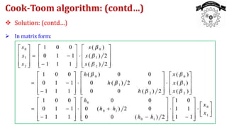
- 27. Solution: (contd…) In matrix form: Cook-Toom algorithm: (contd…)
- 28. Solution: (contd…) The computation is carried out as follows (5 additions, 3 multiplications): Hence the Cook-Toom algorithm needs three multiplications and five additions (ignoring the additions in the pre-computation ), i.e., the number of multiplications is reduced by one at the expense of four extra additions. Cook-Toom algorithm: (contd…)
- 29. Conclusions: Some additions in the pre-addition or post-addition matrices can be shared. So, when we count the number of additions, we count only one, instead of two or three. If we take h0, h1 as the FIR filter coefficients and take x0, x1 as the signal (data) sequence, then the terms H0, H1 need not be recomputed each time the filter is used. They can be precomputed once offline and stored. (So, we ignore these computations when counting the number of operations). Cook-Toom algorithm: (contd…)
- 30. Conclusions: The Cook-Toom algorithm is a matrix decomposition. A convolution can be expressed in matrix-vector forms as: Generally, the equation can be expressed as: Where C is the post-addition matrix, D is the pre-addition matrix, and H is a diagonal matrix with Hi, i = 0, 1, …, (L+N-2) on the main diagonal. Cook-Toom algorithm: (contd…)
- 31. Conclusions: Since T=CHD, it implies that the Cook-Toom algorithm provides a way to factorize the convolution matrix T into multiplication of 1 post-addition matrix C, 1 diagonal matrix H and 1 pre-addition matrix D, such that the total number of multiplications is determined only by the non-zero elements on the main diagonal of the diagonal matrix H (note matrices C and D contain only small integers). Limitations: Although the number of multiplications is reduced, the number of additions has increased. Cook-Toom algorithm: (contd…)
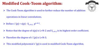
- 32. The Cook-Toom algorithm is used to further reduce the number of addition operations in linear convolutions. Define s' (p) = s(p) - SL+N-2 . pL+N-2. Notice that the degree of s(p) is L+N-2 and SL+N-2 is its highest order coefficient. Therefore the degree of s' (p) is L+N-3. This modified polynomial s’ (p) is used in modified Cook-Toom algorithm. Modified Cook-Toom algorithm:
- 33. Algorithm Description: 1. Choose L+N-2 different real numbers β0, β1, … , βL+N-3 2. Compute h(βi) and x(βi) , for i ={0,1, … , L+N-3} 3. Compute s(βi) = h(βi) . x(βi), for i ={0,1, … , L+N-3} 4. Compute s'(βi) = s(βi)-(sL+N-2).(βi)L+N-2, for i ={0,1, … , L+N-3} Modified Cook-Toom algorithm: (contd…)
- 34. Algorithm Description: 5. Compute s'(p) by using: 6. Compute s(p) = s'(p) + (sL+N-2 ) . (pL+N-2) Modified Cook-Toom algorithm: (contd…)
- 35. Example: Derive a (2X2) convolution algorithm using the modified Cook-Toom algorithm with β={0,-1}. Solution: Consider the Lagrange interpolation for s'(p) = s(p) - h1x1p2 at {β0 = 0, β1 = -1} Find, s'(βi) = h(βi)x(βi) - h1x1βi 2 Find, Modified Cook-Toom algorithm: (contd…)
- 36. Solution: (contd…) Find, This computation requires 2 multiplications {one for h0x0 and another for (h0-h1)(x0- x1); not counting that for h1x1 multiplication}. Apply the Lagrange interpolation algorithm, we get: Modified Cook-Toom algorithm: (contd…)
- 37. Solution: (contd…) Therefore, s( p) = s'( p) + h1x1 p2 = s0 + s1p + s2p2 The corresponding matrix-form expression expressions are: Modified Cook-Toom algorithm: (contd…)
- 38. Solution: (contd…) Modified Cook-Toom algorithm: (contd…)
- 39. Solution: (contd…) The computation is carried out as follows: The total number of operations are 3 multiplications (three in step-3) and 3 additions (one in step-2 and two in step-4). Compared with the linear convolution using Cook-Toom algorithm, the number of addition operations has been reduced by 2 while the number of multiplications remains the same Modified Cook-Toom algorithm: (contd…)
- 40. Conclusions: Limitations: 1. Although the number of multiplications is reduced, the number of additions has increased (As the size of the problem increases, the number of additions increase rapidly). 2. The choices of βi=0, ±1 are good, while the choices of ±2, ±4 (or other small integers) result in complicated pre-addition and post-addition matrices. 3. For larger problems, Cook-Toom algorithm becomes cumbersome. Cook-Toom algorithms:
- 41. The Winograd short convolution algorithm: Based on the CRT (Chinese Remainder Theorem). Chinese Remainder Theorem: It’s possible to uniquely determine a nonnegative integer given its remainder with respect to the given moduli, provided that the moduli are relatively prime and the integer is known to be smaller than the product of the moduli. Winograd Algorithm:
- 42. The Winograd short convolution algorithm: ( contd…) Chinese Remainder Theorem for Integers: Review of Integer Ring: For every integer c and positive integer d, there is a unique pair of integer Q, called the quotient, and integer s, called the remainder; such that c=dQ + s, where 0 ≤ s ≤ d-1. i.e., Q= ⎣ c/d ⎦ and s=Rd[c] Euclidean Algorithm: Given two positive integers s and t, where (t < s), then their Greatest Common Divisor (GCD) can be computed by an iterative application of the division algorithm. Winograd Algorithm: (contd…)
- 43. The Winograd short convolution algorithm: ( contd…) Chinese Remainder Theorem for Integers: (contd…) Euclidean Algorithm: 1. The process stops when a remainder of zero is obtained. 2. The last nonzero remainder t(n) is the GCD(s,t). Winograd Algorithm: (contd…)
- 44. The Winograd short convolution algorithm: ( contd…) Chinese Remainder Theorem for Integers: (contd…) Euclidean Algorithm: In matrix notation: For any integer s and t, there exists integers a and b such that GCD[s, t]= as + bt It is possible to uniquely determine a nonnegative integer given its moduli with respect to each of several integers, provided that the integer is known to be smaller than the product of the moduli. Winograd Algorithm: (contd…)
- 45. The Winograd short convolution algorithm: ( contd…) Chinese Remainder Theorem for Integers: (contd…) Euclidean Algorithm: Example: {m1=3, m2=5} and M=3×5=15 Winograd Algorithm: (contd…)
- 46. The Winograd short convolution algorithm: ( contd…) Chinese Remainder Theorem for Integers: (contd…) Euclidean Algorithm: Example: {m1, m2, m3} = {3, 4, 5} and M = 3× 4 × 5 = 60 Winograd Algorithm: (contd…)
- 47. The Winograd short convolution algorithm: ( contd…) Chinese Remainder Theorem for Integers: (contd…) Given a set of integers m0, m1, … , mk that are pairwise relatively prime (co-prime), then for each integer c, 0 ≤ c < M= m0m1…mk, there is a one-to-one map between c and the vector of residues: (Rm0 [c], Rm1[c], … , Rmk [c]) Conversely, given a set of co-prime integers m0, m1, …, mk and a set of integers c0, c1, …, ck with ci < mi . Then the system of equations ci =c (mod mi), i=0,1,…,k has at most one solution for 0 ≤ c < M. Winograd Algorithm: (contd…)
- 48. The Winograd short convolution algorithm: ( contd…) Chinese Remainder Theorem for Integers: (contd…) Define Mi=M/mi, then GCD[Mi, mi]=1. So there exists integers Ni and ni with GCD[Mi, mi]= 1 = NiMi + nimi, i=0,1,…,k. The system of equations ci=c (mod mi), 0 ≤ I ≤ k, is uniquely solved by: Winograd Algorithm: (contd…)
- 49. The Winograd short convolution algorithm: ( contd…) Chinese Remainder Theorem for Integers: (contd…) Example: GCD Winograd Algorithm: (contd…)
- 50. The Winograd short convolution algorithm: ( contd…) Chinese Remainder Theorem for Integers: (contd…) Given ci = Rmi[c] (represents the remainder when cis divided by mi), for i = 0,1,...,k , where miare moduli and are relatively prime, then c = 𝑖=0 𝑘 𝑐𝑖 NiMi mod M, where M = 𝑖=0 𝑘 𝑚𝑖, Mi = M/mi, and Niis the solution of NiMi + nimi = GCD(Mi, mi)=1, provided that 0 ≤ c < M Winograd Algorithm: (contd…)
- 51. The Winograd short convolution algorithm: ( contd…) Chinese Remainder Theorem for Integers: (contd…) If NiMi + nimi = GCD (Mi, mi) = 1, then we have NiMi= 1 (mod mi). C (mod mi) = 𝑖=0 𝑘 𝑐𝑖𝑁𝑖𝑀𝑖 (𝑚𝑜𝑑 𝑚𝑖) = ci NiMi (mod mi) = ci(mod mi) Winograd Algorithm: (contd…)
- 52. The Winograd short convolution algorithm: ( contd…) Chinese Remainder Theorem (CRT) for Integers: (contd…) Example: Using the CRT for integer, Choose moduli m0=3, m1=4, m2=5. Then M = m0m1m2 = 60 and M i = M/mi By Euclidean theorem, we have: Where and are obtained using the Euclidean GCD algorithm. Given that the integer c satisfy: 0 ≤ c < M, Let ci = Rmi[c] Winograd Algorithm: (contd…)
- 53. The Winograd short convolution algorithm: ( contd…) Chinese Remainder Theorem (CRT) for Integers: (contd…) Example: The integer c can be calculated as: For c=17: Winograd Algorithm: (contd…)
- 54. The Winograd short convolution algorithm: ( contd…) Chinese Remainder Theorem (CRT) for Integers: (contd…) By taking residues, large integers are broken down into small pieces (that may be easy to add and multiply). Examples: Winograd Algorithm: (contd…)
- 55. The Winograd short convolution algorithm: ( contd…) Chinese Remainder Theorem for Polynomials: Winograd Algorithm: (contd…)
- 56. The Winograd short convolution algorithm: ( contd…) Chinese Remainder Theorem for Polynomials: (contd…) Given a set of polynomials m(0)(x), m(1)(x), …, m(k)(x), that are pair-wise relatively prime (co-prime), then for each polynomial c(x), deg(c(x)) < deg(M(x)), M(x)= m(0)(x)m(1)(x)…m(k)(x), there is a one-to-one map between c(x) and the vector of residues: Winograd Algorithm: (contd…)
- 57. The Winograd short convolution algorithm: ( contd…) Chinese Remainder Theorem for Polynomials: (contd…) Conversely, given a set of co-prime polynomials m(0)(x), m(1)(x), …, m(k)(x) and a set of polynomials c(0)(x), c(1)(x), …, c(k)(x) with deg(c(i)(x)) < deg(m(i)(x)). Then the system of equations c(i)(x) =c(x) (mod m(i)(x)), i=0,1,…,k has at most one solution for deg(c(x)) < deg(M(x)). Winograd Algorithm: (contd…)
- 58. The Winograd short convolution algorithm: ( contd…) Chinese Remainder Theorem for Polynomials: (contd…) Define M(i)(x)=M(x)/m(i)(x), then GCD[M(i)(x),m(i)(x)]=1. So there exists polynomials N(i)(x) and n(i)(x) with GCD[M(i)(x), m(i)(x)] = 1 = N(i)(x)M(i)(x) + n(i)(x)m(i)(x), i=0,1,…,k. The system of equations c(i)(x) =c(x) (mod m(i)(x) ), 0 ≤ I ≤ k, is uniquely solved by: Winograd Algorithm: (contd…)
- 59. The Winograd short convolution algorithm: ( contd…) Chinese Remainder Theorem for Polynomials: (contd…) The remainder of a polynomial with regard to modulus xi + f(x), where deg(f(x)) < i, can be evaluated. by substituting xi by –f(x) in the polynomial Example: Winograd Algorithm: (contd…)
- 60. The Winograd short convolution algorithm: ( contd…) Algorithm Description: 1. Choose a polynomial with degree higher than the degree of h(p) x(p ) and factor it into (k+1) relatively prime polynomials with real coefficients, i.e., m(p)= m(0)(p)m(1)(p) … m(k )(p). 2. Let M(i)( p) = m(p)/m(i) (p). Use the Euclidean GCD algorithm to solve N(i)(p)M(i)(p) + n(i)(p)m(i)(p) = 1 for N(i)(p) Winograd Algorithm: (contd…)
- 61. The Winograd short convolution algorithm: ( contd…) Algorithm Description: (contd…) 3. Compute: h(i)(p) = h(p) mod m(i)(p) and x(i)(p) = x(p) mod m(i)(p) for i= 0, 1, …, k. 4. Compute: S(i)(p) = h(i)(p) x(i)(P) mod m(i)(p) for i =0, 1, …, k. 5. Compute s(p) by using: Winograd Algorithm: (contd…)
- 62. The Winograd short convolution algorithm: ( contd…) Example: Consider a (2X3) linear convolution S(p) = h(p)x(p) where h(p) = h0 + h1(p) and x(p) = x0 + x1p + x2p2. Construct an efficient realization using Winograd algorithm with m(p) = p(p-1)(p2+1). Solution: Let m(0)(p) = p, m(1)(p) = (p-1) and m(2)(p) = (p2+1). Construct the following table using the relationships: M(i)(p) = m(p)/m(i)(p) and N(i)(p)M(i)(p) + n(i)(p)m(i)(p) = 1 for i =0, 1, 2. Winograd Algorithm: (contd…)
- 63. The Winograd short convolution algorithm: ( contd…) Solution: (contd…) Compute residues from h(p) = h0 + h1 p and x(p) = x0 + x1p + x2p2: i.e., h(0)(p) = h0 and x(0)(p) = x0. h(1)(p) = h0 + h1 and x(1)(p) = x0 + x1 + x2. h(2)(p) = h0 + h1p and x(2)(p) = (x0 – x2) + x1p. Winograd Algorithm: (contd…) No multiplication operations required
- 64. The Winograd short convolution algorithm: ( contd…) Solution: (contd…) s(0)(p) = h0x0 = s0 (0) s(1)(p) = (h0 + h1)(x0 + x1 + x2) = s0 (1) s(2)(p) = (h0 + h1p)((x0-x2)+x1p) mod(p2+1) = h0(x0-x2)-h1x1+(h0x1+h1(x0-x2))p = s0(2) + s1 (2)p Algorithm complexity: One multiplication for s(0)(p), one for s(1)(p) and four for s(2)(p) Winograd Algorithm: (contd…)
- 65. The Winograd short convolution algorithm: ( contd…) Solution: (contd…) The computational complexity can be reduced to three multiplications as shown below: Then: Winograd Algorithm: (contd…)
- 66. The Winograd short convolution algorithm: ( contd…) Solution: (contd…) Substitute s(0)(p), s(1)(p) and s(2)(p) in the relation for s(p) to obtain the following table: Winograd Algorithm: (contd…)
- 67. The Winograd short convolution algorithm: ( contd…) Solution: (contd…) Therefore, we have: Notice that: Winograd Algorithm: (contd…)
- 68. The Winograd short convolution algorithm: ( contd…) Solution: (contd…) Finally, we have: Here the Winograd convolution algorithm requires five multiplications and 11 additions compared with six multiplications and two additions for direct implementation. Winograd Algorithm: (contd…)
- 69. The Winograd short convolution algorithm: ( contd…) Conclusions: The number of multiplications in Winograd algorithm is highly dependent on the degree of each m(i )( p). Therefore, the degree of m(p) should be as small as possible. More efficient form (or a modified version) of the Winograd algorithm can be obtained by letting deg[m(p)]= deg[s(p)] and applying the CRT to: s’(p) = s(p)-hN-1 . xL-1.m(p) Winograd Algorithm: (contd…)
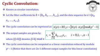
- 70. Known as circular convolution. Let the filter coefficients be h = {h0, h1, … , hn-1}, and the data sequence be x ={x0, x1, … , xn-1}. The cyclic convolution can be expressed as: The output samples are given by: where ((i-k)) denotes (i-k) mod n The cyclic convolution can be computed as a linear convolution reduced by modulo pn – 1 (Notice that there are 2n-1 different output samples for this linear convolution) Cyclic Convolution:
- 71. In circular convolution, coefficients with indices larger than (n-1) are folded back into terms with indices small than n. We can express the cyclic convolution by polynomial product : The circular convolution system is shown below: Cyclic Convolution: (contd…)
- 72. The direct computation of cyclic convolution: Cyclic Convolution: (contd…)
- 73. Alternatively, the cyclic convolution can be computed using CRT with m( p) = pn -1, which is much simpler. Example: Construct a (4X4) cyclic convolution algorithm using CRT with m( p) = p4-1 = (p - 1)(p + 1)(p2 + 1) Solution: Let h( p) = h0 + h1 p + h2 p2 + h p3 and x( p) = x0 + x1 p + x2 p2 + x3 p3 Let m(0 )( p) = p -1, m (1)( p) = p +1 and m(2 )( p) = p2 +1. Cyclic Convolution: (contd…)
- 74. Solution: (contd…) Get the following table using the relationships M (i)(p) = m(p)/m(i)(p) and N (i)(p)M (i)(p) + n (i)(p)m(i)(p) = 1. Cyclic Convolution: (contd…)
- 75. Solution: (contd…) Compute the residues: Cyclic Convolution: (contd…)
- 76. Solution: (contd…) i.e., Individual convolution sum need five multiplications. Cyclic Convolution: (contd…)
- 77. Solution: (contd…) In matrix form: Then: Cyclic Convolution: (contd…)
- 78. Solution: (contd…) So we have: i.e., Cyclic Convolution: (contd…)
- 79. Solution: (contd…) Therefore, we have: This algorithm requires five multiplications and 15 additions. The direct implementation requires 16 multiplications and 12 additions. An efficient cyclic convolution algorithm can often be easily extended to construct efficient linear convolution. Cyclic Convolution: (contd…)
- 80. Solution: (contd…) The direct implementation requires 16 multiplications and 12 additions as shown in the following matrix-form: Notice that the cyclic convolution matrix is a circulant matrix. Cyclic Convolution: (contd…)