SlideShare a Scribd company logo
3
Most read
4
Most read
7
Most read
Chapter 3
Data Mining Techniques
3.1 Introduction
• Parametric models describe the relationship between input and output
through the use of algebraic equations what are some parameters are not
specified. These unspecified parameters are determined by providing input
examples.
• Nonparametric techniques are more appropriate for data mining
applications. A non-parametric model is one that is data-driven. Recent
techniques are able to learn dynamically as data are added to the input.
This dynamic Learning process allows the model to be created
continuously. The more data, the better the model.
• Nonparametric techniques are particularly suitable to the database
applications with large amounts of dynamically changing data.
Nonparametric techniques include neural networks, decision trees, and
genetic algorithms.
3.2 Statistical Perspective. Point Estimation
• The bias of an estimator is the difference between the expected value of the estimator and the actual value. Let 𝐸 Θ denote the
expected value
𝐵𝑖𝑎𝑠 = 𝐸 Θ − Θ = 𝐸 Θ − Θ
• One measure of the effectiveness of an estimate is the mean squared error (MSE), which is the expected value of difference
between the estimates and the actual value:
𝐸 Θ − Θ 2
• The root mean square error (RMSE) is found by taking the square root of the MSE.
• The root mean square (RMS) may also be used to estimate error or as another statistic to describe a distribution. Unlike mean, it
does indicate the magnitude of the values.
𝑅𝑀𝑆 =
𝑗=1
𝑛
𝑥𝑗
2
𝑛
• At popular estimating technique is the jackknife estimate. With this approach, the estimate of a parameter, Θ, is obtained by
omitting one value from the set of observed values. Given set of jackknife estimates, Θ 𝑖 we can obtain an overall estimate
Θ . =
𝑖=1
𝑛
Θ(𝑖)
𝑛
• When we determine a range of values, within which the true parameter value should fall. This range is called a confidence interval.
3.2.2 Estimation and Summarization Models
• Maximum likelihood estimate (MLE) technique for point estimation. The approach obtains parameter estimates that maximize the
probability that that sample data 𝑋 = 𝑥𝑖, … , 𝑥 𝑛 occur for the specific model 𝑓 𝑥𝑖 Θ . The likelihood function is thus defined as
𝐿 Θ 𝑥𝑖, … , 𝑥 𝑛 =
𝑖=1
𝑛
𝑓(𝑥𝑖|Θ) .
The value Θ that maximizes 𝐿 is the estimate chosen. This can be found by taking the derivative with respect to Θ.
• The expectation maximization (EM) algorithm can solve the estimation problem with incomplete data. The EM algorithm finds an
MLE for a parameter (such as a mean) using a two step process: estimation and maximization. These steps are applied iteratively
until successive parameter estimates converge. Such iterative estimates must satisfy
𝜕𝑙𝑛𝐿(Θ|𝑋)
𝜕𝜃𝑖
= 0
• Models based on summarization provide an abstraction and the summarization of the data as a whole. Well-known statistical
concepts such as mean, variance, standard deviation, median, mode are simple models of the underlying population. Fitting
population into a specific frequency distribution provides an even better model of the data.
• Visualization techniques help to display the structure of the data graphically (histograms, box plots, scatter diagrams).
3.2.3 Bayes Theorem
• Bayes rule is a technique to estimate the likelihood of a property given the set of data as evidence or input.
Suppose that either hypothesis ℎ1 or hypothesis ℎ2 must occur and 𝑥𝑖 is an observable event, the Bayes rule
states
𝑃 ℎ1 𝑥𝑖 =
𝑃 𝑥𝑖|ℎ1 𝑃 ℎ1
𝑃 𝑥𝑖|ℎ1 𝑃 ℎ1 + 𝑃 𝑥𝑖|ℎ2 𝑃 ℎ2
• 𝑃 ℎ1 𝑥𝑖 is called the posterior probability, while 𝑃 ℎ1 is the prior probability associated with hypothesis ℎ1. 𝑃 𝑥𝑖
is the probability of the occurrence of data value 𝑥𝑖 and 𝑃 𝑥𝑖|ℎ1 is the conditional probability that, given a
hypothesis the tuple satisfies it. Bayes rule allows to assign probabilities 𝑃 ℎ𝑗 𝑥𝑖 of hypotheses given a data value
𝑃 ℎ1 𝑥𝑖 =
𝑃 𝑥𝑖|ℎ1 𝑃 ℎ1
𝑃 𝑥𝑖
• Hypothesis testing helps to determine if a set of observed variable values is statistically significant (differs
from the expected case). This approach explains the observed data by testing a hypothesis against it. A
hypothesis is first made, then the observed values are compared based on this hypothesis to those of the
expected case. Assuming that 𝑂 represents the observed data and 𝐸 is the expected values based on
hypothesis, the chi-squared statistic, 𝜒2
, is defined as:
𝜒2 =
𝑂 − 𝐸 2
𝐸
3.2.5 Correlations and Regression
• Linear regression assumes that a linear relationship exists between the input and the output data.
The common formula for a linear relationship is:
𝑦 = 𝑐0 + 𝑐1 𝑥1 + ⋯ + 𝑐 𝑛 𝑥 𝑛
• There are: 𝑛 input variables, which are called predictors or regressors; one output variable being
predicted (called a response); 𝑛+1 constants, which are chosen to match model by the input
sample. This is called multiple linear regression because there is more than one predictor.
• Both bivariate regression and correlation can be used to evaluate the strength of a relationship
between two variables.
• One standard formula to measure linear correlation is the correlation coefficient 𝑟 ∈ −1,1 . Here
negative correlation indicates that one variable increases while the other decreases:
𝑟 =
(𝑥𝑖 − 𝑋)(𝑦𝑖 − 𝑌)
(𝑥𝑖 − 𝑋)2 (𝑦𝑖 − 𝑌)2
• When two data variables have a strong correlation, they are similar. Thus, the correlation
coefficient can be used to define similarity for clustering or classification.
3.3 Similarity Measures
Those tuples, that answer the query should be more like each other than those that do not answer it. Each IR query provides the class
definition in the form of the IR query itself. So classification problem then becomes one of determining similarity between each tuple
and the query 𝑂 𝑛 rather than 𝑂 𝑛2
problem. Common similarity measures used:
• Dice 𝑠𝑖𝑚 𝑡𝑖, 𝑡𝑗 =
2 ℎ=1
𝑘
𝑡 𝑖ℎ 𝑡 𝑗ℎ
ℎ=1
𝑘 𝑡 𝑖ℎ
2 + ℎ=1
𝑘 𝑡 𝑗ℎ
2 relates the overlap to the average size of the two sets together
• Jaccard 𝑠𝑖𝑚 𝑡𝑖, 𝑡𝑗 = ℎ=1
𝑘
𝑡 𝑖ℎ 𝑡 𝑗ℎ
ℎ=1
𝑘 𝑡 𝑖ℎ
2 + ℎ=1
𝑘 𝑡 𝑗ℎ
2 − ℎ=1
𝑘 𝑡 𝑖ℎ 𝑡 𝑗ℎ
measures overlap of two sets as related to the whole set caused by their union
• Cosine 𝑠𝑖𝑚 𝑡𝑖, 𝑡𝑗 = ℎ=1
𝑘
𝑡 𝑖ℎ 𝑡 𝑗ℎ
ℎ=1
𝑘 𝑡 𝑖ℎ
2
ℎ=1
𝑘 𝑡 𝑗ℎ
2
relates the overlap to the geometric average of the two sets
• Overlap 𝑠𝑖𝑚 𝑡𝑖, 𝑡𝑗 = ℎ=1
𝑘
𝑡 𝑖ℎ 𝑡 𝑗ℎ
min ℎ=1
𝑘 𝑡 𝑖ℎ
2 , ℎ=1
𝑘 𝑡 𝑗ℎ
2
determines the degree to which two sets overlap
Distance or dissimilarity measure are often used instead of similarity measures. These measure how unlike items are.
• Euclidean 𝑑𝑖𝑠 𝑡𝑖, 𝑡𝑗 = ℎ=1
𝑘
(𝑡𝑖ℎ − 𝑡𝑗ℎ)2
• Manhattan 𝑑𝑖𝑠 𝑡𝑖, 𝑡𝑗 = ℎ=1
𝑘
(𝑡𝑖ℎ−𝑡𝑗ℎ)
Since most similarity measures assume numeric (and often discrete) values, they may be difficult to use for general data types. A
mapping from the attribute domain to a subset of integers may be used and some approach to determining the difference is needed.
3.4 Decision Trees
A decision tree (DT) is a predictive modeling technique used in classification,
clustering, and prediction. A computational DT model consists of three steps:
• A decision tree
• An algorithm to create the tree
• An algorithm that applies the tree to data and solves the problem under
consideration (complexity depends on the product of the number of levels
and the maximum branching factor).
Most decision tree techniques differ in how the tree is created. An algorithm
examines data from a training sample with known classification values in
order to build the tree, or it could be constructed by a domain expert.
3.5 Neural Networks
• The NN can be viewed as directed graph 𝐹 = 𝑉, 𝐴
consisting of vertices and arcs. All the vertices are
partitioned into source(input), sink (output), and
internal (hidden) nodes; every arch 𝑖, 𝑗 is labeled
with a numeric value 𝑤𝑖𝑗; every node 𝑖 is labeled with
a function 𝑓𝑖. The NN as an information processing
system consists of a directed graph and various
algorithms that access the graph.
• NN usually works only with numeric data.
• Artificial NN can be classified based on the type of
connectivity and learning into feed-forward or
feedback, with supervised or unsupervised learning.
• Unlike decision trees, after a tuple is processed, the
NN may be changed to improve future performance.
• NN have a long training time and thus are not
appropriate for real-world applications. NN can be
used in massively parallel systems.
Activation Functions
The output of each node 𝑖 in the NN is based on the definition of an activation function 𝑓𝑖,
associated with it. An activation 𝑓𝑖is applied to the input values 𝑥1𝑖, ⋯ , 𝑥 𝑘𝑖 and weights
𝑤1𝑖, ⋯ , 𝑤 𝑘𝑖 . The inputs are usually combined in a sum of products form 𝑆 = 𝑤ℎ𝑖 𝑥ℎ𝑖 .
The following are alternative definitions for activation function 𝑓𝑖 𝑆 at node 𝑖:
• Linear: 𝑓𝑖 𝑆 = 𝑐𝑆
• Threshold or step: 𝑓𝑖 𝑆 =
1 𝑖𝑓 𝑆 > 𝑇
0 𝑜𝑡ℎ𝑒𝑟𝑤𝑖𝑠𝑒
• Sigmoid: 𝑓𝑖 𝑆 =
1
(1+𝑒−𝑐𝑆)
. This function possesses a simple derivative
𝜕𝑓 𝑖
𝜕𝑆
= 𝑓𝑖 1 − 𝑓𝑖
• Hyperbolic tangent: 𝑓𝑖 𝑆 =
(1−𝑒−𝑆)
(1+𝑒−𝑐𝑆)
• Gaussian: 𝑓𝑖 𝑆 = 𝑒
−𝑆2
𝑣
03 Data Mining Techniques
3.6 Genetic Algorithms
• Initially, a population of individuals 𝑃 is created. They typically are generated randomly. From this
population, a new population 𝑃/ of the same size is created. The algorithm repeatedly selects
individuals from whom to create new ones. These parents (𝑖1, 𝑖2), are then used to produce
offspring or children (𝑜1, 𝑜2) using a crossover process. Then mutants may be generated. The
process continues until the new population satisfies the termination condition.
• A fitness function 𝑓 is used to determine the best individuals in a population. This is then used in
selection process to chose parents to keep. Given an objective by which the population can be
measured, the fitness function indicates how well the goodness objective is being met by an
individual.
• The simplest selections process is to select individuals based on their fitness. Here 𝑝𝐼 𝑖
is the
probability of selecting individual 𝐼𝑖. This type of selection is called roulette wheel selection.
𝑝𝐼 𝑖
=
𝑓(𝐼𝑖)
𝐼 𝑖∈𝑃 𝑓(𝐼𝑗)
• A genetic algorithm (GA) is computational model consisting of five parts: 1) starting set, 2)
crossover technique, 3) mutation algorithm, 4) fitness function, 5) GA algorithm.
References:
Dunham, Margaret H. “Data Mining: Introductory and Advanced
Topics”. Pearson Education, Inc., 2003.

More Related Content

What's hot (20)

PPT
similarity measure
ZHAO Sam
 
PPT
Computational Learning Theory
butest
 
PDF
Digital Image Processing: Image Segmentation
Mostafa G. M. Mostafa
 
PDF
Feature Extraction
skylian
 
PPTX
Image feature extraction
Rushin Shah
 
PPTX
Data mining
Hoang Nguyen
 
PDF
Feature selection
Dong Guo
 
PDF
data mining
manasa polu
 
PPTX
Density based methods
SVijaylakshmi
 
PPTX
R Graphical User Interface Comparison.pptx
Ramakrishna Reddy Bijjam
 
PPT
Digital Image Processing
Reshma KC
 
PPSX
Edge Detection and Segmentation
Dr. A. B. Shinde
 
PPT
Mining Frequent Patterns, Association and Correlations
Justin Cletus
 
PPTX
Hyperparameter Tuning
Jon Lederman
 
PPTX
Genetic algorithms in Data Mining
Atul Khanna
 
PPTX
Dm from databases perspective u 1
sakthyvel3
 
PPT
Knowledge Representation in Artificial intelligence
Yasir Khan
 
PPSX
Color Image Processing: Basics
Dr. A. B. Shinde
 
similarity measure
ZHAO Sam
 
Computational Learning Theory
butest
 
Digital Image Processing: Image Segmentation
Mostafa G. M. Mostafa
 
Feature Extraction
skylian
 
Image feature extraction
Rushin Shah
 
Data mining
Hoang Nguyen
 
Feature selection
Dong Guo
 
data mining
manasa polu
 
Density based methods
SVijaylakshmi
 
R Graphical User Interface Comparison.pptx
Ramakrishna Reddy Bijjam
 
Digital Image Processing
Reshma KC
 
Edge Detection and Segmentation
Dr. A. B. Shinde
 
Mining Frequent Patterns, Association and Correlations
Justin Cletus
 
Hyperparameter Tuning
Jon Lederman
 
Genetic algorithms in Data Mining
Atul Khanna
 
Dm from databases perspective u 1
sakthyvel3
 
Knowledge Representation in Artificial intelligence
Yasir Khan
 
Color Image Processing: Basics
Dr. A. B. Shinde
 

Viewers also liked (20)

PPTX
02 Related Concepts
Valerii Klymchuk
 
PPTX
05 Clustering in Data Mining
Valerii Klymchuk
 
PPTX
Data mining
Akannsha Totewar
 
PPTX
Data Warehouse Project
Valerii Klymchuk
 
PPT
Data Mining Techniques
Houw Liong The
 
PPT
Chapter 10 Data Mining Techniques
Houw Liong The
 
PPT
Chapter 08 Data Mining Techniques
Houw Liong The
 
PPTX
Database Project
Valerii Klymchuk
 
PPTX
04 Classification in Data Mining
Valerii Klymchuk
 
PPTX
01 Introduction to Data Mining
Valerii Klymchuk
 
PPTX
Artificial Intelligence for Automated Decision Support Project
Valerii Klymchuk
 
PPTX
Data mining tools (R , WEKA, RAPID MINER, ORANGE)
Krishna Petrochemicals
 
PPTX
Data Mining: Application and trends in data mining
DataminingTools Inc
 
PDF
Data Mining and Business Intelligence Tools
Motaz Saad
 
PPT
Data Mining Concepts
Dung Nguyen
 
PPT
1.2 steps and functionalities
Krish_ver2
 
PDF
Ghhh
agammya
 
PPTX
Monaco by Saseendranath vs
Saseendranath VS
 
PDF
Análise Pesquisa de Clima
Rafael Perez
 
PPT
Presentacion
Sacnuaj
 
02 Related Concepts
Valerii Klymchuk
 
05 Clustering in Data Mining
Valerii Klymchuk
 
Data mining
Akannsha Totewar
 
Data Warehouse Project
Valerii Klymchuk
 
Data Mining Techniques
Houw Liong The
 
Chapter 10 Data Mining Techniques
Houw Liong The
 
Chapter 08 Data Mining Techniques
Houw Liong The
 
Database Project
Valerii Klymchuk
 
04 Classification in Data Mining
Valerii Klymchuk
 
01 Introduction to Data Mining
Valerii Klymchuk
 
Artificial Intelligence for Automated Decision Support Project
Valerii Klymchuk
 
Data mining tools (R , WEKA, RAPID MINER, ORANGE)
Krishna Petrochemicals
 
Data Mining: Application and trends in data mining
DataminingTools Inc
 
Data Mining and Business Intelligence Tools
Motaz Saad
 
Data Mining Concepts
Dung Nguyen
 
1.2 steps and functionalities
Krish_ver2
 
Ghhh
agammya
 
Monaco by Saseendranath vs
Saseendranath VS
 
Análise Pesquisa de Clima
Rafael Perez
 
Presentacion
Sacnuaj
 
Ad

Similar to 03 Data Mining Techniques (20)

PPTX
Predictive analytics
Dinakar nk
 
PPTX
Unit 3 – AIML.pptx
hiblooms
 
PPT
Supervised and unsupervised learning
AmAn Singh
 
PDF
Machine Learning.pdf
BeyaNasr1
 
PPTX
Ability Study of Proximity Measure for Big Data Mining Context on Clustering
KamleshKumar394
 
PPTX
Cluster analysis
Avijit Famous
 
PPTX
AI & ML(Unit III).pptx.It contains also syllabus
NPRCET6
 
PPTX
Elements of Statistical Learning 読み会 第2章
Tsuyoshi Sakama
 
PPTX
Cluster Analysis
Baivab Nag
 
PPTX
DAM_3Unit.pptx it is used todddddddddddddd
PraneshDeshmukh
 
PPTX
machine learning for engineering students
Kavitabani1
 
PDF
Dr. Shivu___Machine Learning_Module 2pdf
Dr. Shivashankar
 
PPTX
ngboost.pptx
MohamedAliHabib3
 
PDF
Unit-3 Data Analytics.pdf
Sitamarhi Institute of Technology
 
PPTX
Lect 3 background mathematics
hktripathy
 
PDF
L1 statistics
dapdai
 
PPTX
Dimensionality Reduction.pptx
PriyadharshiniG41
 
PPTX
UNIT 3.pptx.......................................
vijayannamratha
 
PDF
Deep learning MindMap
Ashish Patel
 
PPTX
Lect 3 background mathematics for Data Mining
hktripathy
 
Predictive analytics
Dinakar nk
 
Unit 3 – AIML.pptx
hiblooms
 
Supervised and unsupervised learning
AmAn Singh
 
Machine Learning.pdf
BeyaNasr1
 
Ability Study of Proximity Measure for Big Data Mining Context on Clustering
KamleshKumar394
 
Cluster analysis
Avijit Famous
 
AI & ML(Unit III).pptx.It contains also syllabus
NPRCET6
 
Elements of Statistical Learning 読み会 第2章
Tsuyoshi Sakama
 
Cluster Analysis
Baivab Nag
 
DAM_3Unit.pptx it is used todddddddddddddd
PraneshDeshmukh
 
machine learning for engineering students
Kavitabani1
 
Dr. Shivu___Machine Learning_Module 2pdf
Dr. Shivashankar
 
ngboost.pptx
MohamedAliHabib3
 
Unit-3 Data Analytics.pdf
Sitamarhi Institute of Technology
 
Lect 3 background mathematics
hktripathy
 
L1 statistics
dapdai
 
Dimensionality Reduction.pptx
PriyadharshiniG41
 
UNIT 3.pptx.......................................
vijayannamratha
 
Deep learning MindMap
Ashish Patel
 
Lect 3 background mathematics for Data Mining
hktripathy
 
Ad

More from Valerii Klymchuk (7)

PDF
Sample presentation slides template
Valerii Klymchuk
 
PPTX
Toronto Capstone
Valerii Klymchuk
 
PDF
03 Data Representation
Valerii Klymchuk
 
PDF
05 Scalar Visualization
Valerii Klymchuk
 
PDF
06 Vector Visualization
Valerii Klymchuk
 
PDF
07 Tensor Visualization
Valerii Klymchuk
 
PDF
Crime Analysis based on Historical and Transportation Data
Valerii Klymchuk
 
Sample presentation slides template
Valerii Klymchuk
 
Toronto Capstone
Valerii Klymchuk
 
03 Data Representation
Valerii Klymchuk
 
05 Scalar Visualization
Valerii Klymchuk
 
06 Vector Visualization
Valerii Klymchuk
 
07 Tensor Visualization
Valerii Klymchuk
 
Crime Analysis based on Historical and Transportation Data
Valerii Klymchuk
 

Recently uploaded (20)

PPTX
Indigo dyeing Presentation (2).pptx as dye
shreeroop1335
 
PPTX
Presentation by Tariq & Mohammed (1).pptx
AbooddSandoqaa
 
PDF
Kafka Use Cases Real-World Applications
Accentfuture
 
PPTX
Model Evaluation & Visualisation part of a series of intro modules for data ...
brandonlee626749
 
DOCX
Artigo - Playing to Win.planejamento docx
KellyXavier15
 
PPTX
PPT2 W1L2.pptx.........................................
palicteronalyn26
 
DOCX
Cat_Latin_America_in_World_Politics[1].docx
sales480687
 
PPTX
english9quizw1-240228142338-e9bcf6fd.pptx
rossanthonytan130
 
PDF
Blood pressure (3).pdfbdbsbsbhshshshhdhdhshshs
hernandezemma379
 
PPTX
Mynd company all details what they are doing a
AniketKadam40952
 
PPTX
Communication_Skills_Class10_Visual.pptx
namanrastogi70555
 
PDF
624753984-Annex-A3-RPMS-Tool-for-Proficient-Teachers-SY-2024-2025.pdf
CristineGraceAcuyan
 
PDF
Microsoft Power BI - Advanced Certificate for Business Intelligence using Pow...
Prasenjit Debnath
 
PPTX
Monitoring Improvement ( Pomalaa Branch).pptx
fajarkunee
 
DOCX
Starbucks in the Indian market through its joint venture.
sales480687
 
PDF
Orchestrating Data Workloads With Airflow.pdf
ssuserae5511
 
DOCX
brigada_PROGRAM_25.docx the boys white house
RonelNebrao
 
PDF
Informatics Market Insights AI Workforce.pdf
karizaroxx
 
DOCX
Udemy - data management Luisetto Mauro.docx
M. Luisetto Pharm.D.Spec. Pharmacology
 
PDF
NVIDIA Triton Inference Server, a game-changing platform for deploying AI mod...
Tamanna36
 
Indigo dyeing Presentation (2).pptx as dye
shreeroop1335
 
Presentation by Tariq & Mohammed (1).pptx
AbooddSandoqaa
 
Kafka Use Cases Real-World Applications
Accentfuture
 
Model Evaluation & Visualisation part of a series of intro modules for data ...
brandonlee626749
 
Artigo - Playing to Win.planejamento docx
KellyXavier15
 
PPT2 W1L2.pptx.........................................
palicteronalyn26
 
Cat_Latin_America_in_World_Politics[1].docx
sales480687
 
english9quizw1-240228142338-e9bcf6fd.pptx
rossanthonytan130
 
Blood pressure (3).pdfbdbsbsbhshshshhdhdhshshs
hernandezemma379
 
Mynd company all details what they are doing a
AniketKadam40952
 
Communication_Skills_Class10_Visual.pptx
namanrastogi70555
 
624753984-Annex-A3-RPMS-Tool-for-Proficient-Teachers-SY-2024-2025.pdf
CristineGraceAcuyan
 
Microsoft Power BI - Advanced Certificate for Business Intelligence using Pow...
Prasenjit Debnath
 
Monitoring Improvement ( Pomalaa Branch).pptx
fajarkunee
 
Starbucks in the Indian market through its joint venture.
sales480687
 
Orchestrating Data Workloads With Airflow.pdf
ssuserae5511
 
brigada_PROGRAM_25.docx the boys white house
RonelNebrao
 
Informatics Market Insights AI Workforce.pdf
karizaroxx
 
Udemy - data management Luisetto Mauro.docx
M. Luisetto Pharm.D.Spec. Pharmacology
 
NVIDIA Triton Inference Server, a game-changing platform for deploying AI mod...
Tamanna36
 

03 Data Mining Techniques

  • 2. 3.1 Introduction • Parametric models describe the relationship between input and output through the use of algebraic equations what are some parameters are not specified. These unspecified parameters are determined by providing input examples. • Nonparametric techniques are more appropriate for data mining applications. A non-parametric model is one that is data-driven. Recent techniques are able to learn dynamically as data are added to the input. This dynamic Learning process allows the model to be created continuously. The more data, the better the model. • Nonparametric techniques are particularly suitable to the database applications with large amounts of dynamically changing data. Nonparametric techniques include neural networks, decision trees, and genetic algorithms.
  • 3. 3.2 Statistical Perspective. Point Estimation • The bias of an estimator is the difference between the expected value of the estimator and the actual value. Let 𝐸 Θ denote the expected value 𝐵𝑖𝑎𝑠 = 𝐸 Θ − Θ = 𝐸 Θ − Θ • One measure of the effectiveness of an estimate is the mean squared error (MSE), which is the expected value of difference between the estimates and the actual value: 𝐸 Θ − Θ 2 • The root mean square error (RMSE) is found by taking the square root of the MSE. • The root mean square (RMS) may also be used to estimate error or as another statistic to describe a distribution. Unlike mean, it does indicate the magnitude of the values. 𝑅𝑀𝑆 = 𝑗=1 𝑛 𝑥𝑗 2 𝑛 • At popular estimating technique is the jackknife estimate. With this approach, the estimate of a parameter, Θ, is obtained by omitting one value from the set of observed values. Given set of jackknife estimates, Θ 𝑖 we can obtain an overall estimate Θ . = 𝑖=1 𝑛 Θ(𝑖) 𝑛 • When we determine a range of values, within which the true parameter value should fall. This range is called a confidence interval.
  • 4. 3.2.2 Estimation and Summarization Models • Maximum likelihood estimate (MLE) technique for point estimation. The approach obtains parameter estimates that maximize the probability that that sample data 𝑋 = 𝑥𝑖, … , 𝑥 𝑛 occur for the specific model 𝑓 𝑥𝑖 Θ . The likelihood function is thus defined as 𝐿 Θ 𝑥𝑖, … , 𝑥 𝑛 = 𝑖=1 𝑛 𝑓(𝑥𝑖|Θ) . The value Θ that maximizes 𝐿 is the estimate chosen. This can be found by taking the derivative with respect to Θ. • The expectation maximization (EM) algorithm can solve the estimation problem with incomplete data. The EM algorithm finds an MLE for a parameter (such as a mean) using a two step process: estimation and maximization. These steps are applied iteratively until successive parameter estimates converge. Such iterative estimates must satisfy 𝜕𝑙𝑛𝐿(Θ|𝑋) 𝜕𝜃𝑖 = 0 • Models based on summarization provide an abstraction and the summarization of the data as a whole. Well-known statistical concepts such as mean, variance, standard deviation, median, mode are simple models of the underlying population. Fitting population into a specific frequency distribution provides an even better model of the data. • Visualization techniques help to display the structure of the data graphically (histograms, box plots, scatter diagrams).
  • 5. 3.2.3 Bayes Theorem • Bayes rule is a technique to estimate the likelihood of a property given the set of data as evidence or input. Suppose that either hypothesis ℎ1 or hypothesis ℎ2 must occur and 𝑥𝑖 is an observable event, the Bayes rule states 𝑃 ℎ1 𝑥𝑖 = 𝑃 𝑥𝑖|ℎ1 𝑃 ℎ1 𝑃 𝑥𝑖|ℎ1 𝑃 ℎ1 + 𝑃 𝑥𝑖|ℎ2 𝑃 ℎ2 • 𝑃 ℎ1 𝑥𝑖 is called the posterior probability, while 𝑃 ℎ1 is the prior probability associated with hypothesis ℎ1. 𝑃 𝑥𝑖 is the probability of the occurrence of data value 𝑥𝑖 and 𝑃 𝑥𝑖|ℎ1 is the conditional probability that, given a hypothesis the tuple satisfies it. Bayes rule allows to assign probabilities 𝑃 ℎ𝑗 𝑥𝑖 of hypotheses given a data value 𝑃 ℎ1 𝑥𝑖 = 𝑃 𝑥𝑖|ℎ1 𝑃 ℎ1 𝑃 𝑥𝑖 • Hypothesis testing helps to determine if a set of observed variable values is statistically significant (differs from the expected case). This approach explains the observed data by testing a hypothesis against it. A hypothesis is first made, then the observed values are compared based on this hypothesis to those of the expected case. Assuming that 𝑂 represents the observed data and 𝐸 is the expected values based on hypothesis, the chi-squared statistic, 𝜒2 , is defined as: 𝜒2 = 𝑂 − 𝐸 2 𝐸
  • 6. 3.2.5 Correlations and Regression • Linear regression assumes that a linear relationship exists between the input and the output data. The common formula for a linear relationship is: 𝑦 = 𝑐0 + 𝑐1 𝑥1 + ⋯ + 𝑐 𝑛 𝑥 𝑛 • There are: 𝑛 input variables, which are called predictors or regressors; one output variable being predicted (called a response); 𝑛+1 constants, which are chosen to match model by the input sample. This is called multiple linear regression because there is more than one predictor. • Both bivariate regression and correlation can be used to evaluate the strength of a relationship between two variables. • One standard formula to measure linear correlation is the correlation coefficient 𝑟 ∈ −1,1 . Here negative correlation indicates that one variable increases while the other decreases: 𝑟 = (𝑥𝑖 − 𝑋)(𝑦𝑖 − 𝑌) (𝑥𝑖 − 𝑋)2 (𝑦𝑖 − 𝑌)2 • When two data variables have a strong correlation, they are similar. Thus, the correlation coefficient can be used to define similarity for clustering or classification.
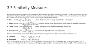
  • 7. 3.3 Similarity Measures Those tuples, that answer the query should be more like each other than those that do not answer it. Each IR query provides the class definition in the form of the IR query itself. So classification problem then becomes one of determining similarity between each tuple and the query 𝑂 𝑛 rather than 𝑂 𝑛2 problem. Common similarity measures used: • Dice 𝑠𝑖𝑚 𝑡𝑖, 𝑡𝑗 = 2 ℎ=1 𝑘 𝑡 𝑖ℎ 𝑡 𝑗ℎ ℎ=1 𝑘 𝑡 𝑖ℎ 2 + ℎ=1 𝑘 𝑡 𝑗ℎ 2 relates the overlap to the average size of the two sets together • Jaccard 𝑠𝑖𝑚 𝑡𝑖, 𝑡𝑗 = ℎ=1 𝑘 𝑡 𝑖ℎ 𝑡 𝑗ℎ ℎ=1 𝑘 𝑡 𝑖ℎ 2 + ℎ=1 𝑘 𝑡 𝑗ℎ 2 − ℎ=1 𝑘 𝑡 𝑖ℎ 𝑡 𝑗ℎ measures overlap of two sets as related to the whole set caused by their union • Cosine 𝑠𝑖𝑚 𝑡𝑖, 𝑡𝑗 = ℎ=1 𝑘 𝑡 𝑖ℎ 𝑡 𝑗ℎ ℎ=1 𝑘 𝑡 𝑖ℎ 2 ℎ=1 𝑘 𝑡 𝑗ℎ 2 relates the overlap to the geometric average of the two sets • Overlap 𝑠𝑖𝑚 𝑡𝑖, 𝑡𝑗 = ℎ=1 𝑘 𝑡 𝑖ℎ 𝑡 𝑗ℎ min ℎ=1 𝑘 𝑡 𝑖ℎ 2 , ℎ=1 𝑘 𝑡 𝑗ℎ 2 determines the degree to which two sets overlap Distance or dissimilarity measure are often used instead of similarity measures. These measure how unlike items are. • Euclidean 𝑑𝑖𝑠 𝑡𝑖, 𝑡𝑗 = ℎ=1 𝑘 (𝑡𝑖ℎ − 𝑡𝑗ℎ)2 • Manhattan 𝑑𝑖𝑠 𝑡𝑖, 𝑡𝑗 = ℎ=1 𝑘 (𝑡𝑖ℎ−𝑡𝑗ℎ) Since most similarity measures assume numeric (and often discrete) values, they may be difficult to use for general data types. A mapping from the attribute domain to a subset of integers may be used and some approach to determining the difference is needed.
  • 8. 3.4 Decision Trees A decision tree (DT) is a predictive modeling technique used in classification, clustering, and prediction. A computational DT model consists of three steps: • A decision tree • An algorithm to create the tree • An algorithm that applies the tree to data and solves the problem under consideration (complexity depends on the product of the number of levels and the maximum branching factor). Most decision tree techniques differ in how the tree is created. An algorithm examines data from a training sample with known classification values in order to build the tree, or it could be constructed by a domain expert.
  • 9. 3.5 Neural Networks • The NN can be viewed as directed graph 𝐹 = 𝑉, 𝐴 consisting of vertices and arcs. All the vertices are partitioned into source(input), sink (output), and internal (hidden) nodes; every arch 𝑖, 𝑗 is labeled with a numeric value 𝑤𝑖𝑗; every node 𝑖 is labeled with a function 𝑓𝑖. The NN as an information processing system consists of a directed graph and various algorithms that access the graph. • NN usually works only with numeric data. • Artificial NN can be classified based on the type of connectivity and learning into feed-forward or feedback, with supervised or unsupervised learning. • Unlike decision trees, after a tuple is processed, the NN may be changed to improve future performance. • NN have a long training time and thus are not appropriate for real-world applications. NN can be used in massively parallel systems.
  • 10. Activation Functions The output of each node 𝑖 in the NN is based on the definition of an activation function 𝑓𝑖, associated with it. An activation 𝑓𝑖is applied to the input values 𝑥1𝑖, ⋯ , 𝑥 𝑘𝑖 and weights 𝑤1𝑖, ⋯ , 𝑤 𝑘𝑖 . The inputs are usually combined in a sum of products form 𝑆 = 𝑤ℎ𝑖 𝑥ℎ𝑖 . The following are alternative definitions for activation function 𝑓𝑖 𝑆 at node 𝑖: • Linear: 𝑓𝑖 𝑆 = 𝑐𝑆 • Threshold or step: 𝑓𝑖 𝑆 = 1 𝑖𝑓 𝑆 > 𝑇 0 𝑜𝑡ℎ𝑒𝑟𝑤𝑖𝑠𝑒 • Sigmoid: 𝑓𝑖 𝑆 = 1 (1+𝑒−𝑐𝑆) . This function possesses a simple derivative 𝜕𝑓 𝑖 𝜕𝑆 = 𝑓𝑖 1 − 𝑓𝑖 • Hyperbolic tangent: 𝑓𝑖 𝑆 = (1−𝑒−𝑆) (1+𝑒−𝑐𝑆) • Gaussian: 𝑓𝑖 𝑆 = 𝑒 −𝑆2 𝑣
  • 12. 3.6 Genetic Algorithms • Initially, a population of individuals 𝑃 is created. They typically are generated randomly. From this population, a new population 𝑃/ of the same size is created. The algorithm repeatedly selects individuals from whom to create new ones. These parents (𝑖1, 𝑖2), are then used to produce offspring or children (𝑜1, 𝑜2) using a crossover process. Then mutants may be generated. The process continues until the new population satisfies the termination condition. • A fitness function 𝑓 is used to determine the best individuals in a population. This is then used in selection process to chose parents to keep. Given an objective by which the population can be measured, the fitness function indicates how well the goodness objective is being met by an individual. • The simplest selections process is to select individuals based on their fitness. Here 𝑝𝐼 𝑖 is the probability of selecting individual 𝐼𝑖. This type of selection is called roulette wheel selection. 𝑝𝐼 𝑖 = 𝑓(𝐼𝑖) 𝐼 𝑖∈𝑃 𝑓(𝐼𝑗) • A genetic algorithm (GA) is computational model consisting of five parts: 1) starting set, 2) crossover technique, 3) mutation algorithm, 4) fitness function, 5) GA algorithm.
  • 13. References: Dunham, Margaret H. “Data Mining: Introductory and Advanced Topics”. Pearson Education, Inc., 2003.