SlideShare a Scribd company logo
Analysis of Algorithms
Basic Graph Algorithms
Andres Mendez-Vazquez
October 28, 2015
1 / 84
Outline
1 Introduction
Graphs Everywhere
History
Basic Theory
Representing Graphs in a Computer
2 Traversing the Graph
Breadth-first search
Depth-First Search
3 Applications
Finding a path between nodes
Connected Components
Spanning Trees
Topological Sorting
2 / 84
Outline
1 Introduction
Graphs Everywhere
History
Basic Theory
Representing Graphs in a Computer
2 Traversing the Graph
Breadth-first search
Depth-First Search
3 Applications
Finding a path between nodes
Connected Components
Spanning Trees
Topological Sorting
3 / 84
We are full of Graphs
Maps
4 / 84
We are full of Graphs
Branch CPU estimators
5 / 84
We are full of Graphs
Social Networks
6 / 84
Outline
1 Introduction
Graphs Everywhere
History
Basic Theory
Representing Graphs in a Computer
2 Traversing the Graph
Breadth-first search
Depth-First Search
3 Applications
Finding a path between nodes
Connected Components
Spanning Trees
Topological Sorting
7 / 84
History
Something Notable
Graph theory started with Euler who was asked to find a nice path across
the seven Königsberg bridges
The Actual City
8 / 84
History
Something Notable
Graph theory started with Euler who was asked to find a nice path across
the seven Königsberg bridges
The Actual City
8 / 84
No solution for a odd number of Bridges
What we want
The (Eulerian) path should cross over each of the seven bridges exactly
once
We cannot do this for the original problem
9 / 84
No solution for a odd number of Bridges
What we want
The (Eulerian) path should cross over each of the seven bridges exactly
once
We cannot do this for the original problem
9 / 84
Necessary Condition
Euler discovered that
A necessary condition for the walk of the desired form is that the graph be
connected and have exactly zero or two nodes of odd degree.
Add an extra bridge
10 / 84
Necessary Condition
Euler discovered that
A necessary condition for the walk of the desired form is that the graph be
connected and have exactly zero or two nodes of odd degree.
Add an extra bridge
Add Extra Bridge
10 / 84
Studying Graphs
All the previous examples are telling us
Data Structures are required to design structures to hold the information
coming from graphs!!!
Good Representations
They will allow to handle the data structures with ease!!!
11 / 84
Studying Graphs
All the previous examples are telling us
Data Structures are required to design structures to hold the information
coming from graphs!!!
Good Representations
They will allow to handle the data structures with ease!!!
11 / 84
Outline
1 Introduction
Graphs Everywhere
History
Basic Theory
Representing Graphs in a Computer
2 Traversing the Graph
Breadth-first search
Depth-First Search
3 Applications
Finding a path between nodes
Connected Components
Spanning Trees
Topological Sorting
12 / 84
Basic Theory
Definition
A Graph is composed of the following parts: Nodes and Edges
Nodes
They can represent multiple things:
People
Cities
States of Being
etc
Edges
They can represent multiple things too:
Distance between cities
Friendships
Matching Strings
Etc
13 / 84
Basic Theory
Definition
A Graph is composed of the following parts: Nodes and Edges
Nodes
They can represent multiple things:
People
Cities
States of Being
etc
Edges
They can represent multiple things too:
Distance between cities
Friendships
Matching Strings
Etc
13 / 84
Basic Theory
Definition
A Graph is composed of the following parts: Nodes and Edges
Nodes
They can represent multiple things:
People
Cities
States of Being
etc
Edges
They can represent multiple things too:
Distance between cities
Friendships
Matching Strings
Etc
13 / 84
Basic Theory
Definition
A Graph is composed of the following parts: Nodes and Edges
Nodes
They can represent multiple things:
People
Cities
States of Being
etc
Edges
They can represent multiple things too:
Distance between cities
Friendships
Matching Strings
Etc
13 / 84
Basic Theory
Definition
A Graph is composed of the following parts: Nodes and Edges
Nodes
They can represent multiple things:
People
Cities
States of Being
etc
Edges
They can represent multiple things too:
Distance between cities
Friendships
Matching Strings
Etc
13 / 84
Basic Theory
Definition
A Graph is composed of the following parts: Nodes and Edges
Nodes
They can represent multiple things:
People
Cities
States of Being
etc
Edges
They can represent multiple things too:
Distance between cities
Friendships
Matching Strings
Etc
13 / 84
Basic Theory
Definition
A Graph is composed of the following parts: Nodes and Edges
Nodes
They can represent multiple things:
People
Cities
States of Being
etc
Edges
They can represent multiple things too:
Distance between cities
Friendships
Matching Strings
Etc
13 / 84
Basic Theory
Definition
A Graph is composed of the following parts: Nodes and Edges
Nodes
They can represent multiple things:
People
Cities
States of Being
etc
Edges
They can represent multiple things too:
Distance between cities
Friendships
Matching Strings
Etc
13 / 84
Basic Theory
Definition
A Graph is composed of the following parts: Nodes and Edges
Nodes
They can represent multiple things:
People
Cities
States of Being
etc
Edges
They can represent multiple things too:
Distance between cities
Friendships
Matching Strings
Etc
13 / 84
Basic Theory
Definition
A Graph is composed of the following parts: Nodes and Edges
Nodes
They can represent multiple things:
People
Cities
States of Being
etc
Edges
They can represent multiple things too:
Distance between cities
Friendships
Matching Strings
Etc
13 / 84
Basic Theory
Definition
A graph G = (V , E) is composed of a set of vertices (or nodes) V and a
set of edges E, each assumed finite i.e. |V | = n and |E| = m.
Example
14 / 84
Basic Theory
Definition
A graph G = (V , E) is composed of a set of vertices (or nodes) V and a
set of edges E, each assumed finite i.e. |V | = n and |E| = m.
Example
14 / 84
Properties
Incident
An edge ek = (vi, vj) is incident with the vertices vi and vj.
A simple graph has no self-loops or multiple edges like below
15 / 84
Properties
Incident
An edge ek = (vi, vj) is incident with the vertices vi and vj.
A simple graph has no self-loops or multiple edges like below
15 / 84
Some properties
Degree
The degree d(v) of a vertex V is its number of incident edges
A self loop
A self-loop counts for 2 in the degree function.
Proposition
The sum of the degrees of a graph G = (V , E) equals 2|E| = 2m (trivial).
16 / 84
Some properties
Degree
The degree d(v) of a vertex V is its number of incident edges
A self loop
A self-loop counts for 2 in the degree function.
Proposition
The sum of the degrees of a graph G = (V , E) equals 2|E| = 2m (trivial).
16 / 84
Some properties
Degree
The degree d(v) of a vertex V is its number of incident edges
A self loop
A self-loop counts for 2 in the degree function.
Proposition
The sum of the degrees of a graph G = (V , E) equals 2|E| = 2m (trivial).
16 / 84
Some properties
Complete
A complete graph Kn is a simple graph with all n(n−1)/2 possible edges,
like the graph below for n = 2, 3, 4, 5.
Example
17 / 84
Some properties
Complete
A complete graph Kn is a simple graph with all n(n−1)/2 possible edges,
like the graph below for n = 2, 3, 4, 5.
Example
17 / 84
Outline
1 Introduction
Graphs Everywhere
History
Basic Theory
Representing Graphs in a Computer
2 Traversing the Graph
Breadth-first search
Depth-First Search
3 Applications
Finding a path between nodes
Connected Components
Spanning Trees
Topological Sorting
18 / 84
Clearly
We need to represent
Nodes
Vertices
We need to represent
Directed edges
Undirected edges
19 / 84
Clearly
We need to represent
Nodes
Vertices
We need to represent
Directed edges
Undirected edges
19 / 84
We need NICE representations of this definition
First One
Adjacency Representation
Second One
Matrix Representation
20 / 84
We need NICE representations of this definition
First One
Adjacency Representation
Second One
Matrix Representation
20 / 84
Adjacency-list representation
Basic Definition
It is an array of size |V| with
A list for each bucket representing a node telling us which nodes are
connected to it by one edge
21 / 84
Adjacency-list representation
Basic Definition
It is an array of size |V| with
A list for each bucket representing a node telling us which nodes are
connected to it by one edge
1
2
3
4
5
6
4
4 6
4
5
1
2
2 3 5
21 / 84
Properties
Space for storage
For undirected or directed graphs O (V + E)
Search: Successful or Unsuccessful
O(1 + degree(v))
In addition
Adjacency lists can readily be adapted to represent weighted graphs
Weight function w : E → R
The weight w(u, v) of the edge (u, v) ∈ E is simply stored with
vertex v in u’s adjacency list
22 / 84
Possible Disadvantage
When looking to see if an edge exist
There is no quicker way to determine if a given edge (u,v)
23 / 84
Adjacency Matrix Representation
In a natural way the edges can be identified by the nodes
For example, the edge between 1 and 4 nodes gets named as (1,4)
Then
How, we use this to represent the graph through a Matrix or and Array of
Arrays??!!!
24 / 84
Adjacency Matrix Representation
In a natural way the edges can be identified by the nodes
For example, the edge between 1 and 4 nodes gets named as (1,4)
Then
How, we use this to represent the graph through a Matrix or and Array of
Arrays??!!!
24 / 84
What about the following?
How do we indicate that an edge exist given the following matrix
1 2 3 4 5 6
1 − − − − − −
2 − − − − − −
3 − − − − − −
4 − − − − − −
5 − − − − − −
6 − − − − − −
You say it!!
Use a 0 for no-edge
Use a 1 for edge
25 / 84
What about the following?
How do we indicate that an edge exist given the following matrix
1 2 3 4 5 6
1 − − − − − −
2 − − − − − −
3 − − − − − −
4 − − − − − −
5 − − − − − −
6 − − − − − −
You say it!!
Use a 0 for no-edge
Use a 1 for edge
25 / 84
We have then...
Definition
0/1 N × N matrix with N =Number of nodes or vertices
A(i, j) = 1 iff (i, j) is an edge
26 / 84
We have then...
For the previous example
1 2 3 4 5 6
1 0 0 0 1 0 0
2 0 0 0 1 0 0
3 0 0 0 1 0 0
4 1 1 1 0 1 0
5 0 0 0 1 0 1
6 0 0 0 0 1 0
27 / 84
Properties of the Matrix for Undirected Graphs
Property One
Diagonal entries are zero.
Property Two
Adjacency matrix of an undirected graph is symmetric:
A (i, j) = A (j, i) for all i and j
28 / 84
Properties of the Matrix for Undirected Graphs
Property One
Diagonal entries are zero.
Property Two
Adjacency matrix of an undirected graph is symmetric:
A (i, j) = A (j, i) for all i and j
28 / 84
Complexity
Memory
Θ (V 2) (1)
Looking for an edge
O(1)
29 / 84
Complexity
Memory
Θ (V 2) (1)
Looking for an edge
O(1)
29 / 84
Traversing the Graph
Why do we need to traverse the graph?
Do you have any examples?
Yes
Search for paths satisfying various constraints
Shortest Path
Visit some sets of vertices
Tours
Search if two graphs are equivalent
Isomorphisms
30 / 84
Traversing the Graph
Why do we need to traverse the graph?
Do you have any examples?
Yes
Search for paths satisfying various constraints
Shortest Path
Visit some sets of vertices
Tours
Search if two graphs are equivalent
Isomorphisms
30 / 84
Traversing the Graph
Why do we need to traverse the graph?
Do you have any examples?
Yes
Search for paths satisfying various constraints
Shortest Path
Visit some sets of vertices
Tours
Search if two graphs are equivalent
Isomorphisms
30 / 84
Traversing the Graph
Why do we need to traverse the graph?
Do you have any examples?
Yes
Search for paths satisfying various constraints
Shortest Path
Visit some sets of vertices
Tours
Search if two graphs are equivalent
Isomorphisms
30 / 84
Outline
1 Introduction
Graphs Everywhere
History
Basic Theory
Representing Graphs in a Computer
2 Traversing the Graph
Breadth-first search
Depth-First Search
3 Applications
Finding a path between nodes
Connected Components
Spanning Trees
Topological Sorting
31 / 84
Breadth-first search
Definition
Given a graph G = (V , E) and a source vertex s, breadth-first search
systematically explores the edges of Gto “discover” every vertex that is
reachable from the vertex s
Something Notable
A vertex is discovered the first time it is encountered during the search
32 / 84
Breadth-First Search Algorithm
Algorithm
BFS(G, s)
1. for each vertex u ∈ G.V − {s}
2. u.color = WHITE
3. u.d = ∞
4. u.π = NIL
5. s.color =GRAY
6. s.d = 0
7. s.π = NIL
8. Q = ∅
9. Enqueue(Q, s)
10. while Q = ∅
11. u =Dequeue(Q)
12. for each v ∈ G.Adj [u]
13. if v.color ==WHITE
14. v.color =GRAY
15. v.d = u.d + 1
16. v.π = u
17. Enqueue(Q, v)
18. u.color = BLACK
33 / 84
BFS allows to change the order of recursion
Remember
1
2
3 4
5
6
34 / 84
Loop Invariance
The While loop
This while loop maintains the following invariant :
At the test in line 10, the queue Q consists of the set of gray vertices
First iteration
Q = sand s.color = GRAY
Maintenance
The inner loop only pushes gray nodes into the queue.
35 / 84
Loop Invariance
The While loop
This while loop maintains the following invariant :
At the test in line 10, the queue Q consists of the set of gray vertices
First iteration
Q = sand s.color = GRAY
Maintenance
The inner loop only pushes gray nodes into the queue.
35 / 84
Loop Invariance
The While loop
This while loop maintains the following invariant :
At the test in line 10, the queue Q consists of the set of gray vertices
First iteration
Q = sand s.color = GRAY
Maintenance
The inner loop only pushes gray nodes into the queue.
35 / 84
Loop Invariance
Termination
When every node that can be visited is painted black
36 / 84
Example
What do you see?
0
0
37 / 84
Example
What do you see?
0
1 1
1
1
38 / 84
Example
What do you see?
0
1 2
1
12
39 / 84
Example
What do you see?
0
2 2 2
1
12
2
2
40 / 84
Example
What do you see?
0
2 2
1
12
2
2
41 / 84
Example
What do you see?
0
2 3
1
12
2
2
3
42 / 84
Example
What do you see?
0
3 3
1
12
2
2
3
3
43 / 84
Example
What do you see?
0
3
1
12
2
2
3
3
44 / 84
Example
What do you see?
01
12
2
2
3
3
45 / 84
Complexity
What about the outer loop?
O(V ) Enqueue / Dequeue operations – Each adjacency list is processed
only once.
What about the inner loop?
The sum of the lengths of f all the adjacency lists is Θ(E) so the scanning
takes O(E)
46 / 84
Complexity
What about the outer loop?
O(V ) Enqueue / Dequeue operations – Each adjacency list is processed
only once.
What about the inner loop?
The sum of the lengths of f all the adjacency lists is Θ(E) so the scanning
takes O(E)
46 / 84
Complexity
Overhead of Creation
O (V )
Then
Total complexity O (V + E)
47 / 84
Complexity
Overhead of Creation
O (V )
Then
Total complexity O (V + E)
47 / 84
Properties: Predecessor Graph
Something Notable
Breadth-first search constructs a breadth-first tree, initially containing only
its root, which is the source vertex s
Thus
We say that u is the predecessor or parent of v in the breadth-first tree.
48 / 84
Properties: Predecessor Graph
Something Notable
Breadth-first search constructs a breadth-first tree, initially containing only
its root, which is the source vertex s
Thus
We say that u is the predecessor or parent of v in the breadth-first tree.
48 / 84
For example
From the previous example
Predecessor Graph
49 / 84
For example
From the previous example
Predecessor Graph
s
r w
v t x
yu
49 / 84
This allow to use the Algorithm for finding The Shortest
Path
Clearly
This is the unweighted version or all weights are equal!!!
We have the following function
δ (s, v)= shortest path from s to v
We claim that
Upon termination of BFS, every vertex v ∈ V reachable from s has
v.d = δ(s, v)
50 / 84
This allow to use the Algorithm for finding The Shortest
Path
Clearly
This is the unweighted version or all weights are equal!!!
We have the following function
δ (s, v)= shortest path from s to v
We claim that
Upon termination of BFS, every vertex v ∈ V reachable from s has
v.d = δ(s, v)
50 / 84
This allow to use the Algorithm for finding The Shortest
Path
Clearly
This is the unweighted version or all weights are equal!!!
We have the following function
δ (s, v)= shortest path from s to v
We claim that
Upon termination of BFS, every vertex v ∈ V reachable from s has
v.d = δ(s, v)
50 / 84
Intuitive Idea of Claim
Correctness of breadth-first search
Let G = (V , E) be a directed or undirected graph.
Suppose that BFS is run on G from a given source vertex s ∈ V .
Then
Then, during its execution, BFS discovers every vertex v ∈ V that is
reachable from the source.
51 / 84
Intuitive Idea of Claim
Correctness of breadth-first search
Let G = (V , E) be a directed or undirected graph.
Suppose that BFS is run on G from a given source vertex s ∈ V .
Then
Then, during its execution, BFS discovers every vertex v ∈ V that is
reachable from the source.
51 / 84
Intuitive Idea of Claim
Correctness of breadth-first search
Let G = (V , E) be a directed or undirected graph.
Suppose that BFS is run on G from a given source vertex s ∈ V .
Then
Then, during its execution, BFS discovers every vertex v ∈ V that is
reachable from the source.
51 / 84
Intuitive Idea of Claim
Distance Idea
First, once a node u is reached from v, we use the previous shortest
distance from s to update the node distance.
52 / 84
Intuitive Idea of Claim
You can use the idea of strong induction
Given a branch of the breadth-first search u s, u1, u2, ..., un
un.π = un−1.π + 1 = un−1.π + 2 = n + s.π = n (2)
Thus, we have that
For any vertex v = s that is reachable from s, one of the shortest
path from s to v is
A shortest path from s to v.π followed by thew edge (v.π, v).
53 / 84
Outline
1 Introduction
Graphs Everywhere
History
Basic Theory
Representing Graphs in a Computer
2 Traversing the Graph
Breadth-first search
Depth-First Search
3 Applications
Finding a path between nodes
Connected Components
Spanning Trees
Topological Sorting
54 / 84
Depth-first search
Given G
Pick an unvisited vertex v, remember the rest.
Recurse on vertices adjacent to v
55 / 84
The Pseudo-code
Code for DFS
DFS(G)
1. for each vertex u ∈ G.V
2. u.color = WHITE
3. u.π = NIL
4. time = 0
5. for each vertex u ∈ G.V
6. if u.color = WHITE
7.
DFS-VISIT(G, u)
DFS-VISIT(G, u)
1. time = time + 1
2. u.d = time
3. u.color = GRAY
4. for each vertex v ∈ G.Adj [u]
5. if v.color == WHITE
6. v.π = u
7. DFS-VISIT(G, v)
8. u.color = BLACK
9. time = time + 1
10. u.f = time
56 / 84
Example
What do we do?
57 / 84
Example
What do we do?
58 / 84
Example
What do we do?
59 / 84
Example
What do we do?
60 / 84
Example
What do we do?
61 / 84
Example
What do we do?
62 / 84
Example
What do we do?
63 / 84
Example
What do we do?
64 / 84
Complexity
Analysis
1 The loops on lines 1–3 and lines 5–7 of DFS take Θ (V ).
2 The procedure DFS-VISIT is called exactly once for each vertex
v ∈ V .
3 During an execution of DFS-VISIT(G, v) the loop on lines 4–7
executes |Adj (v)| times.
4 But v∈V |Adj (v)| = Θ (E) we have that the cost of executing g
lines 4–7 of DFS-VISIT is Θ (E) .
Then
DFS complexity is Θ (V + E)
65 / 84
Applications
We have several
Topological Sort
Strongly Connected Components
Computer Vision Algorithms
Artificial Intelligence Algorithms
Importance in Social Network
Rank Algorithms for Google
Etc.
66 / 84
Applications
We have several
Topological Sort
Strongly Connected Components
Computer Vision Algorithms
Artificial Intelligence Algorithms
Importance in Social Network
Rank Algorithms for Google
Etc.
66 / 84
Applications
We have several
Topological Sort
Strongly Connected Components
Computer Vision Algorithms
Artificial Intelligence Algorithms
Importance in Social Network
Rank Algorithms for Google
Etc.
66 / 84
Applications
We have several
Topological Sort
Strongly Connected Components
Computer Vision Algorithms
Artificial Intelligence Algorithms
Importance in Social Network
Rank Algorithms for Google
Etc.
66 / 84
Applications
We have several
Topological Sort
Strongly Connected Components
Computer Vision Algorithms
Artificial Intelligence Algorithms
Importance in Social Network
Rank Algorithms for Google
Etc.
66 / 84
Applications
We have several
Topological Sort
Strongly Connected Components
Computer Vision Algorithms
Artificial Intelligence Algorithms
Importance in Social Network
Rank Algorithms for Google
Etc.
66 / 84
Applications
We have several
Topological Sort
Strongly Connected Components
Computer Vision Algorithms
Artificial Intelligence Algorithms
Importance in Social Network
Rank Algorithms for Google
Etc.
66 / 84
Outline
1 Introduction
Graphs Everywhere
History
Basic Theory
Representing Graphs in a Computer
2 Traversing the Graph
Breadth-first search
Depth-First Search
3 Applications
Finding a path between nodes
Connected Components
Spanning Trees
Topological Sorting
67 / 84
Finding a path between nodes
We do the following
Start a breadth-first search at vertex v.
Terminate when vertex u is visited or when Q becomes empty
(whichever occurs first).
Time Complexity
O V 2 when adjacency matrix used.
O(V + E) when adjacency lists used.
68 / 84
Finding a path between nodes
We do the following
Start a breadth-first search at vertex v.
Terminate when vertex u is visited or when Q becomes empty
(whichever occurs first).
Time Complexity
O V 2 when adjacency matrix used.
O(V + E) when adjacency lists used.
68 / 84
Finding a path between nodes
We do the following
Start a breadth-first search at vertex v.
Terminate when vertex u is visited or when Q becomes empty
(whichever occurs first).
Time Complexity
O V 2 when adjacency matrix used.
O(V + E) when adjacency lists used.
68 / 84
Finding a path between nodes
We do the following
Start a breadth-first search at vertex v.
Terminate when vertex u is visited or when Q becomes empty
(whichever occurs first).
Time Complexity
O V 2 when adjacency matrix used.
O(V + E) when adjacency lists used.
68 / 84
This allow to use the Algorithm for finding The Shortest
Path
Clearly
This is the unweighted version or all weights are equal!!!
We have the following function
δ (s, v)= shortest path from s to v
Actually
Upon termination of BFS, every vertex v ∈ V reachable from s has
distance(v) = δ(s, v)
69 / 84
This allow to use the Algorithm for finding The Shortest
Path
Clearly
This is the unweighted version or all weights are equal!!!
We have the following function
δ (s, v)= shortest path from s to v
Actually
Upon termination of BFS, every vertex v ∈ V reachable from s has
distance(v) = δ(s, v)
69 / 84
This allow to use the Algorithm for finding The Shortest
Path
Clearly
This is the unweighted version or all weights are equal!!!
We have the following function
δ (s, v)= shortest path from s to v
Actually
Upon termination of BFS, every vertex v ∈ V reachable from s has
distance(v) = δ(s, v)
69 / 84
Outline
1 Introduction
Graphs Everywhere
History
Basic Theory
Representing Graphs in a Computer
2 Traversing the Graph
Breadth-first search
Depth-First Search
3 Applications
Finding a path between nodes
Connected Components
Spanning Trees
Topological Sorting
70 / 84
Connected Components
Definition
A connected component (or just component) of an undirected graph is a
subgraph in which any two vertices are connected to each other by paths.
Example
71 / 84
Connected Components
Definition
A connected component (or just component) of an undirected graph is a
subgraph in which any two vertices are connected to each other by paths.
Example
71 / 84
Procedure
First
Start a breadth-first search at any as yet unvisited vertex of the graph.
Thus
Newly visited vertices (plus edges between them) define a component.
Repeat
Repeat until all vertices are visited.
72 / 84
Procedure
First
Start a breadth-first search at any as yet unvisited vertex of the graph.
Thus
Newly visited vertices (plus edges between them) define a component.
Repeat
Repeat until all vertices are visited.
72 / 84
Procedure
First
Start a breadth-first search at any as yet unvisited vertex of the graph.
Thus
Newly visited vertices (plus edges between them) define a component.
Repeat
Repeat until all vertices are visited.
72 / 84
Time
O (V 2
)
When adjacency matrix used
O(V + E)
When adjacency lists used (E is number of edges)
73 / 84
Time
O (V 2
)
When adjacency matrix used
O(V + E)
When adjacency lists used (E is number of edges)
73 / 84
Outline
1 Introduction
Graphs Everywhere
History
Basic Theory
Representing Graphs in a Computer
2 Traversing the Graph
Breadth-first search
Depth-First Search
3 Applications
Finding a path between nodes
Connected Components
Spanning Trees
Topological Sorting
74 / 84
Spanning Tree with edges with same weight of no weight
Definition
A spanning tree of a graph G = (V , E) is a acyclic graph where for
u, v ∈ V , there is a path between them
Example
75 / 84
Spanning Tree with edges with same weight of no weight
Definition
A spanning tree of a graph G = (V , E) is a acyclic graph where for
u, v ∈ V , there is a path between them
Example
2
3
5
1
4
6
7
9
8
75 / 84
Procedure
First
Start a breadth-first search at any vertex of the graph.
Thus
If graph is connected, the n − 1 edges used to get to unvisited vertices
define a spanning tree (breadth-first spanning tree).
76 / 84
Procedure
First
Start a breadth-first search at any vertex of the graph.
Thus
If graph is connected, the n − 1 edges used to get to unvisited vertices
define a spanning tree (breadth-first spanning tree).
76 / 84
Time
O (V 2
)
When adjacency matrix used
O(V + E)
When adjacency lists used (E is number of edges)
77 / 84
Time
O (V 2
)
When adjacency matrix used
O(V + E)
When adjacency lists used (E is number of edges)
77 / 84
Outline
1 Introduction
Graphs Everywhere
History
Basic Theory
Representing Graphs in a Computer
2 Traversing the Graph
Breadth-first search
Depth-First Search
3 Applications
Finding a path between nodes
Connected Components
Spanning Trees
Topological Sorting
78 / 84
Topological Sorting
Definitions
A topological sort (sometimes abbreviated topsort or toposort) or
topological ordering of a directed graph is a linear ordering of its vertices
such that for every directed edge (u, v) from vertex u to vertex y, u comes
before v in the ordering.
From Industrial Engineering
The canonical application of topological sorting (topological order) is
in scheduling a sequence of jobs or tasks based on their dependencies.
Topological sorting algorithms were first studied in the early 1960s in
the context of the PERT technique for scheduling in project
management (Jarnagin 1960).
79 / 84
Then
We have that
The jobs are represented by vertices, and there is an edge from x to y if
job x must be completed before job y can be started.
Example
When washing clothes, the washing machine must finish before we put the
clothes to dry.
Then
A topological sort gives an order in which to perform the jobs.
80 / 84
Then
We have that
The jobs are represented by vertices, and there is an edge from x to y if
job x must be completed before job y can be started.
Example
When washing clothes, the washing machine must finish before we put the
clothes to dry.
Then
A topological sort gives an order in which to perform the jobs.
80 / 84
Algorithm
Pseudo Code
TOPOLOGICAL-SORT
1 Call DFS(G) to compute finishing times v.f for each vertex v.
2 As each vertex is finished, insert it onto the front of a linked list
3 Return the linked list of vertices
81 / 84
Algorithm
Pseudo Code
TOPOLOGICAL-SORT
1 Call DFS(G) to compute finishing times v.f for each vertex v.
2 As each vertex is finished, insert it onto the front of a linked list
3 Return the linked list of vertices
81 / 84
Algorithm
Pseudo Code
TOPOLOGICAL-SORT
1 Call DFS(G) to compute finishing times v.f for each vertex v.
2 As each vertex is finished, insert it onto the front of a linked list
3 Return the linked list of vertices
81 / 84
Example
Dressing
undershort
socks
pants
belt
shirt
tie
jacket
shoes
watch
11/16
12/15
6/7
1/8
2/5
3/4
17/18
13/14
u.d/u.f
9/10
82 / 84
Thus
Using the u.f
As each vertex is finished, insert it onto the front of a
linked list
83 / 84
Example
After Sorting
undershortsocks pants beltshirt tie jacketshoes watch
11/16 12/15 6/71/8 2/5 3/417/18 13/14 9/10
84 / 84
Ad

More Related Content

What's hot (20)

Binomial Heap
Binomial HeapBinomial Heap
Binomial Heap
Goa App
 
Approximation Algorithms
Approximation AlgorithmsApproximation Algorithms
Approximation Algorithms
Nicolas Bettenburg
 
Graph theory
Graph theory Graph theory
Graph theory
iranian translate
 
Dijkstra s algorithm
Dijkstra s algorithmDijkstra s algorithm
Dijkstra s algorithm
mansab MIRZA
 
Fp growth
Fp growthFp growth
Fp growth
Farah M. Altufaili
 
BFS
BFSBFS
BFS
jyothimonc
 
Knapsack Problem
Knapsack ProblemKnapsack Problem
Knapsack Problem
Jenny Galino
 
Depth-First Search
Depth-First SearchDepth-First Search
Depth-First Search
Dakshitha Dissanayaka
 
Graph coloring and_applications
Graph coloring and_applicationsGraph coloring and_applications
Graph coloring and_applications
mohammad alkhalil
 
Elliptical curve cryptography
Elliptical curve cryptographyElliptical curve cryptography
Elliptical curve cryptography
Barani Tharan
 
dijkstra algo.ppt
dijkstra algo.pptdijkstra algo.ppt
dijkstra algo.ppt
Santhosh Krishna
 
Dijkstra’S Algorithm
Dijkstra’S AlgorithmDijkstra’S Algorithm
Dijkstra’S Algorithm
ami_01
 
Ch4b
Ch4bCh4b
Ch4b
kinnarshah8888
 
Data Structure and Algorithms Hashing
Data Structure and Algorithms HashingData Structure and Algorithms Hashing
Data Structure and Algorithms Hashing
ManishPrajapati78
 
Algorithms Lecture 7: Graph Algorithms
Algorithms Lecture 7: Graph AlgorithmsAlgorithms Lecture 7: Graph Algorithms
Algorithms Lecture 7: Graph Algorithms
Mohamed Loey
 
RSA Algorithm
RSA AlgorithmRSA Algorithm
RSA Algorithm
chauhankapil
 
graph theory
graph theory graph theory
graph theory
ganith2k13
 
Directed Acyclic Graph
Directed Acyclic Graph Directed Acyclic Graph
Directed Acyclic Graph
AJAL A J
 
Breadth first search and depth first search
Breadth first search and  depth first searchBreadth first search and  depth first search
Breadth first search and depth first search
Hossain Md Shakhawat
 
Slides Chapter10.1 10.2
Slides Chapter10.1 10.2Slides Chapter10.1 10.2
Slides Chapter10.1 10.2
showslidedump
 

Viewers also liked (20)

Distributed Graph Algorithms
Distributed Graph AlgorithmsDistributed Graph Algorithms
Distributed Graph Algorithms
Saurav Kumar
 
Graph theory
Graph theoryGraph theory
Graph theory
Kumar
 
17 Disjoint Set Representation
17 Disjoint Set Representation17 Disjoint Set Representation
17 Disjoint Set Representation
Andres Mendez-Vazquez
 
1535 graph algorithms
1535 graph algorithms1535 graph algorithms
1535 graph algorithms
Dr Fereidoun Dejahang
 
Union find
Union findUnion find
Union find
Vyakhya Shrivastava
 
Topological Sort
Topological SortTopological Sort
Topological Sort
Dr Sandeep Kumar Poonia
 
Advanced Algorithms #1 - Union/Find on Disjoint-set Data Structures.
Advanced Algorithms #1 - Union/Find on Disjoint-set Data Structures.Advanced Algorithms #1 - Union/Find on Disjoint-set Data Structures.
Advanced Algorithms #1 - Union/Find on Disjoint-set Data Structures.
Andrea Angella
 
Graph Traversal Algorithm
Graph Traversal AlgorithmGraph Traversal Algorithm
Graph Traversal Algorithm
jyothimonc
 
07. disjoint set
07. disjoint set07. disjoint set
07. disjoint set
Onkar Nath Sharma
 
Disjoint sets
Disjoint setsDisjoint sets
Disjoint sets
Core Condor
 
Huffman tree
Huffman tree Huffman tree
Huffman tree
Al-amin Hossain
 
Fano algorithm
Fano algorithmFano algorithm
Fano algorithm
Hrudya Balachandran
 
Sets and disjoint sets union123
Sets and disjoint sets union123Sets and disjoint sets union123
Sets and disjoint sets union123
Ankita Goyal
 
Binary Search Tree
Binary Search TreeBinary Search Tree
Binary Search Tree
GowriKumar Chandramouli
 
Graph Traversal Algorithms - Depth First Search Traversal
Graph Traversal Algorithms - Depth First Search TraversalGraph Traversal Algorithms - Depth First Search Traversal
Graph Traversal Algorithms - Depth First Search Traversal
Amrinder Arora
 
Shannon Fano
Shannon FanoShannon Fano
Shannon Fano
anithabalaprabhu
 
2.2 topological sort 02
2.2 topological sort 022.2 topological sort 02
2.2 topological sort 02
Krish_ver2
 
Set data structure
Set data structure Set data structure
Set data structure
Tech_MX
 
DFS and BFS
DFS and BFSDFS and BFS
DFS and BFS
satya parsana
 
Graphs bfs dfs
Graphs bfs dfsGraphs bfs dfs
Graphs bfs dfs
Jaya Gautam
 
Ad

Similar to 18 Basic Graph Algorithms (20)

Graphs and eularian circuit & path with c++ program
Graphs and eularian circuit & path with c++ programGraphs and eularian circuit & path with c++ program
Graphs and eularian circuit & path with c++ program
Muhammad Danish Badar
 
Graph Analytics - From the Whiteboard to Your Toolbox - Sam Lerma
Graph Analytics - From the Whiteboard to Your Toolbox - Sam LermaGraph Analytics - From the Whiteboard to Your Toolbox - Sam Lerma
Graph Analytics - From the Whiteboard to Your Toolbox - Sam Lerma
PyData
 
Lecture 5b graphs and hashing
Lecture 5b graphs and hashingLecture 5b graphs and hashing
Lecture 5b graphs and hashing
Victor Palmar
 
Introduction to Graph Theory
Introduction to Graph TheoryIntroduction to Graph Theory
Introduction to Graph Theory
Premsankar Chakkingal
 
Data Structure of computer science and technology
Data Structure of computer science and technologyData Structure of computer science and technology
Data Structure of computer science and technology
bhaskarsai499
 
Preparation Data Structures 11 graphs
Preparation Data Structures 11 graphsPreparation Data Structures 11 graphs
Preparation Data Structures 11 graphs
Andres Mendez-Vazquez
 
graph_theory_1-11.pdf___________________
graph_theory_1-11.pdf___________________graph_theory_1-11.pdf___________________
graph_theory_1-11.pdf___________________
ssuser1989da
 
Data Structures and Agorithm: DS 21 Graph Theory.pptx
Data Structures and Agorithm: DS 21 Graph Theory.pptxData Structures and Agorithm: DS 21 Graph Theory.pptx
Data Structures and Agorithm: DS 21 Graph Theory.pptx
RashidFaridChishti
 
Breadth first search
Breadth first searchBreadth first search
Breadth first search
Sazzad Hossain
 
Graphs
GraphsGraphs
Graphs
KomalPaliwal3
 
graph representation.pdf
graph representation.pdfgraph representation.pdf
graph representation.pdf
amitbhachne
 
Graph ASS DBATU.pptx
Graph ASS DBATU.pptxGraph ASS DBATU.pptx
Graph ASS DBATU.pptx
ARVIND SARDAR
 
LEC 12-DSALGO-GRAPHS(final12).pdf
LEC 12-DSALGO-GRAPHS(final12).pdfLEC 12-DSALGO-GRAPHS(final12).pdf
LEC 12-DSALGO-GRAPHS(final12).pdf
MuhammadUmerIhtisham
 
graph.pptx
graph.pptxgraph.pptx
graph.pptx
hijigaf
 
Graphs in Data Structure
 Graphs in Data Structure Graphs in Data Structure
Graphs in Data Structure
hafsa komal
 
lecture 17
lecture 17lecture 17
lecture 17
sajinsc
 
Graph Theory
Graph TheoryGraph Theory
Graph Theory
kailash shaw
 
Lecture 2.3.1 Graph.pptx
Lecture 2.3.1 Graph.pptxLecture 2.3.1 Graph.pptx
Lecture 2.3.1 Graph.pptx
king779879
 
graph ASS (1).ppt
graph ASS (1).pptgraph ASS (1).ppt
graph ASS (1).ppt
ARVIND SARDAR
 
graphass1-23022111180722548-1ba6b00a.ppt
graphass1-23022111180722548-1ba6b00a.pptgraphass1-23022111180722548-1ba6b00a.ppt
graphass1-23022111180722548-1ba6b00a.ppt
ssuser7b9bda1
 
Graphs and eularian circuit & path with c++ program
Graphs and eularian circuit & path with c++ programGraphs and eularian circuit & path with c++ program
Graphs and eularian circuit & path with c++ program
Muhammad Danish Badar
 
Graph Analytics - From the Whiteboard to Your Toolbox - Sam Lerma
Graph Analytics - From the Whiteboard to Your Toolbox - Sam LermaGraph Analytics - From the Whiteboard to Your Toolbox - Sam Lerma
Graph Analytics - From the Whiteboard to Your Toolbox - Sam Lerma
PyData
 
Lecture 5b graphs and hashing
Lecture 5b graphs and hashingLecture 5b graphs and hashing
Lecture 5b graphs and hashing
Victor Palmar
 
Data Structure of computer science and technology
Data Structure of computer science and technologyData Structure of computer science and technology
Data Structure of computer science and technology
bhaskarsai499
 
Preparation Data Structures 11 graphs
Preparation Data Structures 11 graphsPreparation Data Structures 11 graphs
Preparation Data Structures 11 graphs
Andres Mendez-Vazquez
 
graph_theory_1-11.pdf___________________
graph_theory_1-11.pdf___________________graph_theory_1-11.pdf___________________
graph_theory_1-11.pdf___________________
ssuser1989da
 
Data Structures and Agorithm: DS 21 Graph Theory.pptx
Data Structures and Agorithm: DS 21 Graph Theory.pptxData Structures and Agorithm: DS 21 Graph Theory.pptx
Data Structures and Agorithm: DS 21 Graph Theory.pptx
RashidFaridChishti
 
graph representation.pdf
graph representation.pdfgraph representation.pdf
graph representation.pdf
amitbhachne
 
Graph ASS DBATU.pptx
Graph ASS DBATU.pptxGraph ASS DBATU.pptx
Graph ASS DBATU.pptx
ARVIND SARDAR
 
graph.pptx
graph.pptxgraph.pptx
graph.pptx
hijigaf
 
Graphs in Data Structure
 Graphs in Data Structure Graphs in Data Structure
Graphs in Data Structure
hafsa komal
 
lecture 17
lecture 17lecture 17
lecture 17
sajinsc
 
Lecture 2.3.1 Graph.pptx
Lecture 2.3.1 Graph.pptxLecture 2.3.1 Graph.pptx
Lecture 2.3.1 Graph.pptx
king779879
 
graphass1-23022111180722548-1ba6b00a.ppt
graphass1-23022111180722548-1ba6b00a.pptgraphass1-23022111180722548-1ba6b00a.ppt
graphass1-23022111180722548-1ba6b00a.ppt
ssuser7b9bda1
 
Ad

More from Andres Mendez-Vazquez (20)

2.03 bayesian estimation
2.03 bayesian estimation2.03 bayesian estimation
2.03 bayesian estimation
Andres Mendez-Vazquez
 
05 linear transformations
05 linear transformations05 linear transformations
05 linear transformations
Andres Mendez-Vazquez
 
01.04 orthonormal basis_eigen_vectors
01.04 orthonormal basis_eigen_vectors01.04 orthonormal basis_eigen_vectors
01.04 orthonormal basis_eigen_vectors
Andres Mendez-Vazquez
 
01.03 squared matrices_and_other_issues
01.03 squared matrices_and_other_issues01.03 squared matrices_and_other_issues
01.03 squared matrices_and_other_issues
Andres Mendez-Vazquez
 
01.02 linear equations
01.02 linear equations01.02 linear equations
01.02 linear equations
Andres Mendez-Vazquez
 
01.01 vector spaces
01.01 vector spaces01.01 vector spaces
01.01 vector spaces
Andres Mendez-Vazquez
 
06 recurrent neural_networks
06 recurrent neural_networks06 recurrent neural_networks
06 recurrent neural_networks
Andres Mendez-Vazquez
 
05 backpropagation automatic_differentiation
05 backpropagation automatic_differentiation05 backpropagation automatic_differentiation
05 backpropagation automatic_differentiation
Andres Mendez-Vazquez
 
Zetta global
Zetta globalZetta global
Zetta global
Andres Mendez-Vazquez
 
01 Introduction to Neural Networks and Deep Learning
01 Introduction to Neural Networks and Deep Learning01 Introduction to Neural Networks and Deep Learning
01 Introduction to Neural Networks and Deep Learning
Andres Mendez-Vazquez
 
25 introduction reinforcement_learning
25 introduction reinforcement_learning25 introduction reinforcement_learning
25 introduction reinforcement_learning
Andres Mendez-Vazquez
 
Neural Networks and Deep Learning Syllabus
Neural Networks and Deep Learning SyllabusNeural Networks and Deep Learning Syllabus
Neural Networks and Deep Learning Syllabus
Andres Mendez-Vazquez
 
Introduction to artificial_intelligence_syllabus
Introduction to artificial_intelligence_syllabusIntroduction to artificial_intelligence_syllabus
Introduction to artificial_intelligence_syllabus
Andres Mendez-Vazquez
 
Ideas 09 22_2018
Ideas 09 22_2018Ideas 09 22_2018
Ideas 09 22_2018
Andres Mendez-Vazquez
 
Ideas about a Bachelor in Machine Learning/Data Sciences
Ideas about a Bachelor in Machine Learning/Data SciencesIdeas about a Bachelor in Machine Learning/Data Sciences
Ideas about a Bachelor in Machine Learning/Data Sciences
Andres Mendez-Vazquez
 
Analysis of Algorithms Syllabus
Analysis of Algorithms  SyllabusAnalysis of Algorithms  Syllabus
Analysis of Algorithms Syllabus
Andres Mendez-Vazquez
 
20 k-means, k-center, k-meoids and variations
20 k-means, k-center, k-meoids and variations20 k-means, k-center, k-meoids and variations
20 k-means, k-center, k-meoids and variations
Andres Mendez-Vazquez
 
18.1 combining models
18.1 combining models18.1 combining models
18.1 combining models
Andres Mendez-Vazquez
 
17 vapnik chervonenkis dimension
17 vapnik chervonenkis dimension17 vapnik chervonenkis dimension
17 vapnik chervonenkis dimension
Andres Mendez-Vazquez
 
A basic introduction to learning
A basic introduction to learningA basic introduction to learning
A basic introduction to learning
Andres Mendez-Vazquez
 
01.04 orthonormal basis_eigen_vectors
01.04 orthonormal basis_eigen_vectors01.04 orthonormal basis_eigen_vectors
01.04 orthonormal basis_eigen_vectors
Andres Mendez-Vazquez
 
01.03 squared matrices_and_other_issues
01.03 squared matrices_and_other_issues01.03 squared matrices_and_other_issues
01.03 squared matrices_and_other_issues
Andres Mendez-Vazquez
 
05 backpropagation automatic_differentiation
05 backpropagation automatic_differentiation05 backpropagation automatic_differentiation
05 backpropagation automatic_differentiation
Andres Mendez-Vazquez
 
01 Introduction to Neural Networks and Deep Learning
01 Introduction to Neural Networks and Deep Learning01 Introduction to Neural Networks and Deep Learning
01 Introduction to Neural Networks and Deep Learning
Andres Mendez-Vazquez
 
25 introduction reinforcement_learning
25 introduction reinforcement_learning25 introduction reinforcement_learning
25 introduction reinforcement_learning
Andres Mendez-Vazquez
 
Neural Networks and Deep Learning Syllabus
Neural Networks and Deep Learning SyllabusNeural Networks and Deep Learning Syllabus
Neural Networks and Deep Learning Syllabus
Andres Mendez-Vazquez
 
Introduction to artificial_intelligence_syllabus
Introduction to artificial_intelligence_syllabusIntroduction to artificial_intelligence_syllabus
Introduction to artificial_intelligence_syllabus
Andres Mendez-Vazquez
 
Ideas about a Bachelor in Machine Learning/Data Sciences
Ideas about a Bachelor in Machine Learning/Data SciencesIdeas about a Bachelor in Machine Learning/Data Sciences
Ideas about a Bachelor in Machine Learning/Data Sciences
Andres Mendez-Vazquez
 
20 k-means, k-center, k-meoids and variations
20 k-means, k-center, k-meoids and variations20 k-means, k-center, k-meoids and variations
20 k-means, k-center, k-meoids and variations
Andres Mendez-Vazquez
 

Recently uploaded (20)

The Gaussian Process Modeling Module in UQLab
The Gaussian Process Modeling Module in UQLabThe Gaussian Process Modeling Module in UQLab
The Gaussian Process Modeling Module in UQLab
Journal of Soft Computing in Civil Engineering
 
new ppt artificial intelligence historyyy
new ppt artificial intelligence historyyynew ppt artificial intelligence historyyy
new ppt artificial intelligence historyyy
PianoPianist
 
introduction to machine learining for beginers
introduction to machine learining for beginersintroduction to machine learining for beginers
introduction to machine learining for beginers
JoydebSheet
 
Level 1-Safety.pptx Presentation of Electrical Safety
Level 1-Safety.pptx Presentation of Electrical SafetyLevel 1-Safety.pptx Presentation of Electrical Safety
Level 1-Safety.pptx Presentation of Electrical Safety
JoseAlbertoCariasDel
 
π0.5: a Vision-Language-Action Model with Open-World Generalization
π0.5: a Vision-Language-Action Model with Open-World Generalizationπ0.5: a Vision-Language-Action Model with Open-World Generalization
π0.5: a Vision-Language-Action Model with Open-World Generalization
NABLAS株式会社
 
AI-assisted Software Testing (3-hours tutorial)
AI-assisted Software Testing (3-hours tutorial)AI-assisted Software Testing (3-hours tutorial)
AI-assisted Software Testing (3-hours tutorial)
Vəhid Gəruslu
 
Explainable-Artificial-Intelligence-XAI-A-Deep-Dive (1).pptx
Explainable-Artificial-Intelligence-XAI-A-Deep-Dive (1).pptxExplainable-Artificial-Intelligence-XAI-A-Deep-Dive (1).pptx
Explainable-Artificial-Intelligence-XAI-A-Deep-Dive (1).pptx
MahaveerVPandit
 
Machine learning project on employee attrition detection using (2).pptx
Machine learning project on employee attrition detection using (2).pptxMachine learning project on employee attrition detection using (2).pptx
Machine learning project on employee attrition detection using (2).pptx
rajeswari89780
 
Structural Response of Reinforced Self-Compacting Concrete Deep Beam Using Fi...
Structural Response of Reinforced Self-Compacting Concrete Deep Beam Using Fi...Structural Response of Reinforced Self-Compacting Concrete Deep Beam Using Fi...
Structural Response of Reinforced Self-Compacting Concrete Deep Beam Using Fi...
Journal of Soft Computing in Civil Engineering
 
"Boiler Feed Pump (BFP): Working, Applications, Advantages, and Limitations E...
"Boiler Feed Pump (BFP): Working, Applications, Advantages, and Limitations E..."Boiler Feed Pump (BFP): Working, Applications, Advantages, and Limitations E...
"Boiler Feed Pump (BFP): Working, Applications, Advantages, and Limitations E...
Infopitaara
 
DT REPORT by Tech titan GROUP to introduce the subject design Thinking
DT REPORT by Tech titan GROUP to introduce the subject design ThinkingDT REPORT by Tech titan GROUP to introduce the subject design Thinking
DT REPORT by Tech titan GROUP to introduce the subject design Thinking
DhruvChotaliya2
 
Oil-gas_Unconventional oil and gass_reseviours.pdf
Oil-gas_Unconventional oil and gass_reseviours.pdfOil-gas_Unconventional oil and gass_reseviours.pdf
Oil-gas_Unconventional oil and gass_reseviours.pdf
M7md3li2
 
Development of MLR, ANN and ANFIS Models for Estimation of PCUs at Different ...
Development of MLR, ANN and ANFIS Models for Estimation of PCUs at Different ...Development of MLR, ANN and ANFIS Models for Estimation of PCUs at Different ...
Development of MLR, ANN and ANFIS Models for Estimation of PCUs at Different ...
Journal of Soft Computing in Civil Engineering
 
Lidar for Autonomous Driving, LiDAR Mapping for Driverless Cars.pptx
Lidar for Autonomous Driving, LiDAR Mapping for Driverless Cars.pptxLidar for Autonomous Driving, LiDAR Mapping for Driverless Cars.pptx
Lidar for Autonomous Driving, LiDAR Mapping for Driverless Cars.pptx
RishavKumar530754
 
Artificial Intelligence (AI) basics.pptx
Artificial Intelligence (AI) basics.pptxArtificial Intelligence (AI) basics.pptx
Artificial Intelligence (AI) basics.pptx
aditichinar
 
fluke dealers in bangalore..............
fluke dealers in bangalore..............fluke dealers in bangalore..............
fluke dealers in bangalore..............
Haresh Vaswani
 
International Journal of Distributed and Parallel systems (IJDPS)
International Journal of Distributed and Parallel systems (IJDPS)International Journal of Distributed and Parallel systems (IJDPS)
International Journal of Distributed and Parallel systems (IJDPS)
samueljackson3773
 
five-year-soluhhhhhhhhhhhhhhhhhtions.pdf
five-year-soluhhhhhhhhhhhhhhhhhtions.pdffive-year-soluhhhhhhhhhhhhhhhhhtions.pdf
five-year-soluhhhhhhhhhhhhhhhhhtions.pdf
AdityaSharma944496
 
Fort night presentation new0903 pdf.pdf.
Fort night presentation new0903 pdf.pdf.Fort night presentation new0903 pdf.pdf.
Fort night presentation new0903 pdf.pdf.
anuragmk56
 
Smart_Storage_Systems_Production_Engineering.pptx
Smart_Storage_Systems_Production_Engineering.pptxSmart_Storage_Systems_Production_Engineering.pptx
Smart_Storage_Systems_Production_Engineering.pptx
rushikeshnavghare94
 
new ppt artificial intelligence historyyy
new ppt artificial intelligence historyyynew ppt artificial intelligence historyyy
new ppt artificial intelligence historyyy
PianoPianist
 
introduction to machine learining for beginers
introduction to machine learining for beginersintroduction to machine learining for beginers
introduction to machine learining for beginers
JoydebSheet
 
Level 1-Safety.pptx Presentation of Electrical Safety
Level 1-Safety.pptx Presentation of Electrical SafetyLevel 1-Safety.pptx Presentation of Electrical Safety
Level 1-Safety.pptx Presentation of Electrical Safety
JoseAlbertoCariasDel
 
π0.5: a Vision-Language-Action Model with Open-World Generalization
π0.5: a Vision-Language-Action Model with Open-World Generalizationπ0.5: a Vision-Language-Action Model with Open-World Generalization
π0.5: a Vision-Language-Action Model with Open-World Generalization
NABLAS株式会社
 
AI-assisted Software Testing (3-hours tutorial)
AI-assisted Software Testing (3-hours tutorial)AI-assisted Software Testing (3-hours tutorial)
AI-assisted Software Testing (3-hours tutorial)
Vəhid Gəruslu
 
Explainable-Artificial-Intelligence-XAI-A-Deep-Dive (1).pptx
Explainable-Artificial-Intelligence-XAI-A-Deep-Dive (1).pptxExplainable-Artificial-Intelligence-XAI-A-Deep-Dive (1).pptx
Explainable-Artificial-Intelligence-XAI-A-Deep-Dive (1).pptx
MahaveerVPandit
 
Machine learning project on employee attrition detection using (2).pptx
Machine learning project on employee attrition detection using (2).pptxMachine learning project on employee attrition detection using (2).pptx
Machine learning project on employee attrition detection using (2).pptx
rajeswari89780
 
"Boiler Feed Pump (BFP): Working, Applications, Advantages, and Limitations E...
"Boiler Feed Pump (BFP): Working, Applications, Advantages, and Limitations E..."Boiler Feed Pump (BFP): Working, Applications, Advantages, and Limitations E...
"Boiler Feed Pump (BFP): Working, Applications, Advantages, and Limitations E...
Infopitaara
 
DT REPORT by Tech titan GROUP to introduce the subject design Thinking
DT REPORT by Tech titan GROUP to introduce the subject design ThinkingDT REPORT by Tech titan GROUP to introduce the subject design Thinking
DT REPORT by Tech titan GROUP to introduce the subject design Thinking
DhruvChotaliya2
 
Oil-gas_Unconventional oil and gass_reseviours.pdf
Oil-gas_Unconventional oil and gass_reseviours.pdfOil-gas_Unconventional oil and gass_reseviours.pdf
Oil-gas_Unconventional oil and gass_reseviours.pdf
M7md3li2
 
Lidar for Autonomous Driving, LiDAR Mapping for Driverless Cars.pptx
Lidar for Autonomous Driving, LiDAR Mapping for Driverless Cars.pptxLidar for Autonomous Driving, LiDAR Mapping for Driverless Cars.pptx
Lidar for Autonomous Driving, LiDAR Mapping for Driverless Cars.pptx
RishavKumar530754
 
Artificial Intelligence (AI) basics.pptx
Artificial Intelligence (AI) basics.pptxArtificial Intelligence (AI) basics.pptx
Artificial Intelligence (AI) basics.pptx
aditichinar
 
fluke dealers in bangalore..............
fluke dealers in bangalore..............fluke dealers in bangalore..............
fluke dealers in bangalore..............
Haresh Vaswani
 
International Journal of Distributed and Parallel systems (IJDPS)
International Journal of Distributed and Parallel systems (IJDPS)International Journal of Distributed and Parallel systems (IJDPS)
International Journal of Distributed and Parallel systems (IJDPS)
samueljackson3773
 
five-year-soluhhhhhhhhhhhhhhhhhtions.pdf
five-year-soluhhhhhhhhhhhhhhhhhtions.pdffive-year-soluhhhhhhhhhhhhhhhhhtions.pdf
five-year-soluhhhhhhhhhhhhhhhhhtions.pdf
AdityaSharma944496
 
Fort night presentation new0903 pdf.pdf.
Fort night presentation new0903 pdf.pdf.Fort night presentation new0903 pdf.pdf.
Fort night presentation new0903 pdf.pdf.
anuragmk56
 
Smart_Storage_Systems_Production_Engineering.pptx
Smart_Storage_Systems_Production_Engineering.pptxSmart_Storage_Systems_Production_Engineering.pptx
Smart_Storage_Systems_Production_Engineering.pptx
rushikeshnavghare94
 

18 Basic Graph Algorithms

  • 1. Analysis of Algorithms Basic Graph Algorithms Andres Mendez-Vazquez October 28, 2015 1 / 84
  • 2. Outline 1 Introduction Graphs Everywhere History Basic Theory Representing Graphs in a Computer 2 Traversing the Graph Breadth-first search Depth-First Search 3 Applications Finding a path between nodes Connected Components Spanning Trees Topological Sorting 2 / 84
  • 3. Outline 1 Introduction Graphs Everywhere History Basic Theory Representing Graphs in a Computer 2 Traversing the Graph Breadth-first search Depth-First Search 3 Applications Finding a path between nodes Connected Components Spanning Trees Topological Sorting 3 / 84
  • 4. We are full of Graphs Maps 4 / 84
  • 5. We are full of Graphs Branch CPU estimators 5 / 84
  • 6. We are full of Graphs Social Networks 6 / 84
  • 7. Outline 1 Introduction Graphs Everywhere History Basic Theory Representing Graphs in a Computer 2 Traversing the Graph Breadth-first search Depth-First Search 3 Applications Finding a path between nodes Connected Components Spanning Trees Topological Sorting 7 / 84
  • 8. History Something Notable Graph theory started with Euler who was asked to find a nice path across the seven Königsberg bridges The Actual City 8 / 84
  • 9. History Something Notable Graph theory started with Euler who was asked to find a nice path across the seven Königsberg bridges The Actual City 8 / 84
  • 10. No solution for a odd number of Bridges What we want The (Eulerian) path should cross over each of the seven bridges exactly once We cannot do this for the original problem 9 / 84
  • 11. No solution for a odd number of Bridges What we want The (Eulerian) path should cross over each of the seven bridges exactly once We cannot do this for the original problem 9 / 84
  • 12. Necessary Condition Euler discovered that A necessary condition for the walk of the desired form is that the graph be connected and have exactly zero or two nodes of odd degree. Add an extra bridge 10 / 84
  • 13. Necessary Condition Euler discovered that A necessary condition for the walk of the desired form is that the graph be connected and have exactly zero or two nodes of odd degree. Add an extra bridge Add Extra Bridge 10 / 84
  • 14. Studying Graphs All the previous examples are telling us Data Structures are required to design structures to hold the information coming from graphs!!! Good Representations They will allow to handle the data structures with ease!!! 11 / 84
  • 15. Studying Graphs All the previous examples are telling us Data Structures are required to design structures to hold the information coming from graphs!!! Good Representations They will allow to handle the data structures with ease!!! 11 / 84
  • 16. Outline 1 Introduction Graphs Everywhere History Basic Theory Representing Graphs in a Computer 2 Traversing the Graph Breadth-first search Depth-First Search 3 Applications Finding a path between nodes Connected Components Spanning Trees Topological Sorting 12 / 84
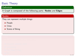
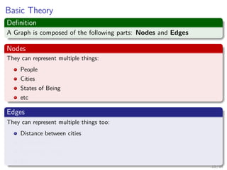
  • 17. Basic Theory Definition A Graph is composed of the following parts: Nodes and Edges Nodes They can represent multiple things: People Cities States of Being etc Edges They can represent multiple things too: Distance between cities Friendships Matching Strings Etc 13 / 84
  • 18. Basic Theory Definition A Graph is composed of the following parts: Nodes and Edges Nodes They can represent multiple things: People Cities States of Being etc Edges They can represent multiple things too: Distance between cities Friendships Matching Strings Etc 13 / 84
  • 19. Basic Theory Definition A Graph is composed of the following parts: Nodes and Edges Nodes They can represent multiple things: People Cities States of Being etc Edges They can represent multiple things too: Distance between cities Friendships Matching Strings Etc 13 / 84
  • 20. Basic Theory Definition A Graph is composed of the following parts: Nodes and Edges Nodes They can represent multiple things: People Cities States of Being etc Edges They can represent multiple things too: Distance between cities Friendships Matching Strings Etc 13 / 84
  • 21. Basic Theory Definition A Graph is composed of the following parts: Nodes and Edges Nodes They can represent multiple things: People Cities States of Being etc Edges They can represent multiple things too: Distance between cities Friendships Matching Strings Etc 13 / 84
  • 22. Basic Theory Definition A Graph is composed of the following parts: Nodes and Edges Nodes They can represent multiple things: People Cities States of Being etc Edges They can represent multiple things too: Distance between cities Friendships Matching Strings Etc 13 / 84
  • 23. Basic Theory Definition A Graph is composed of the following parts: Nodes and Edges Nodes They can represent multiple things: People Cities States of Being etc Edges They can represent multiple things too: Distance between cities Friendships Matching Strings Etc 13 / 84
  • 24. Basic Theory Definition A Graph is composed of the following parts: Nodes and Edges Nodes They can represent multiple things: People Cities States of Being etc Edges They can represent multiple things too: Distance between cities Friendships Matching Strings Etc 13 / 84
  • 25. Basic Theory Definition A Graph is composed of the following parts: Nodes and Edges Nodes They can represent multiple things: People Cities States of Being etc Edges They can represent multiple things too: Distance between cities Friendships Matching Strings Etc 13 / 84
  • 26. Basic Theory Definition A Graph is composed of the following parts: Nodes and Edges Nodes They can represent multiple things: People Cities States of Being etc Edges They can represent multiple things too: Distance between cities Friendships Matching Strings Etc 13 / 84
  • 27. Basic Theory Definition A graph G = (V , E) is composed of a set of vertices (or nodes) V and a set of edges E, each assumed finite i.e. |V | = n and |E| = m. Example 14 / 84
  • 28. Basic Theory Definition A graph G = (V , E) is composed of a set of vertices (or nodes) V and a set of edges E, each assumed finite i.e. |V | = n and |E| = m. Example 14 / 84
  • 29. Properties Incident An edge ek = (vi, vj) is incident with the vertices vi and vj. A simple graph has no self-loops or multiple edges like below 15 / 84
  • 30. Properties Incident An edge ek = (vi, vj) is incident with the vertices vi and vj. A simple graph has no self-loops or multiple edges like below 15 / 84
  • 31. Some properties Degree The degree d(v) of a vertex V is its number of incident edges A self loop A self-loop counts for 2 in the degree function. Proposition The sum of the degrees of a graph G = (V , E) equals 2|E| = 2m (trivial). 16 / 84
  • 32. Some properties Degree The degree d(v) of a vertex V is its number of incident edges A self loop A self-loop counts for 2 in the degree function. Proposition The sum of the degrees of a graph G = (V , E) equals 2|E| = 2m (trivial). 16 / 84
  • 33. Some properties Degree The degree d(v) of a vertex V is its number of incident edges A self loop A self-loop counts for 2 in the degree function. Proposition The sum of the degrees of a graph G = (V , E) equals 2|E| = 2m (trivial). 16 / 84
  • 34. Some properties Complete A complete graph Kn is a simple graph with all n(n−1)/2 possible edges, like the graph below for n = 2, 3, 4, 5. Example 17 / 84
  • 35. Some properties Complete A complete graph Kn is a simple graph with all n(n−1)/2 possible edges, like the graph below for n = 2, 3, 4, 5. Example 17 / 84
  • 36. Outline 1 Introduction Graphs Everywhere History Basic Theory Representing Graphs in a Computer 2 Traversing the Graph Breadth-first search Depth-First Search 3 Applications Finding a path between nodes Connected Components Spanning Trees Topological Sorting 18 / 84
  • 37. Clearly We need to represent Nodes Vertices We need to represent Directed edges Undirected edges 19 / 84
  • 38. Clearly We need to represent Nodes Vertices We need to represent Directed edges Undirected edges 19 / 84
  • 39. We need NICE representations of this definition First One Adjacency Representation Second One Matrix Representation 20 / 84
  • 40. We need NICE representations of this definition First One Adjacency Representation Second One Matrix Representation 20 / 84
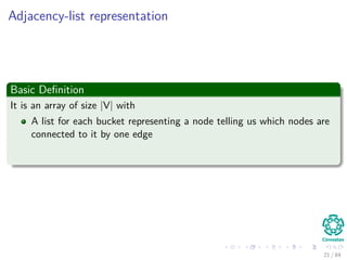
  • 41. Adjacency-list representation Basic Definition It is an array of size |V| with A list for each bucket representing a node telling us which nodes are connected to it by one edge 21 / 84
  • 42. Adjacency-list representation Basic Definition It is an array of size |V| with A list for each bucket representing a node telling us which nodes are connected to it by one edge 1 2 3 4 5 6 4 4 6 4 5 1 2 2 3 5 21 / 84
  • 43. Properties Space for storage For undirected or directed graphs O (V + E) Search: Successful or Unsuccessful O(1 + degree(v)) In addition Adjacency lists can readily be adapted to represent weighted graphs Weight function w : E → R The weight w(u, v) of the edge (u, v) ∈ E is simply stored with vertex v in u’s adjacency list 22 / 84
  • 44. Properties Space for storage For undirected or directed graphs O (V + E) Search: Successful or Unsuccessful O(1 + degree(v)) In addition Adjacency lists can readily be adapted to represent weighted graphs Weight function w : E → R The weight w(u, v) of the edge (u, v) ∈ E is simply stored with vertex v in u’s adjacency list 22 / 84
  • 45. Properties Space for storage For undirected or directed graphs O (V + E) Search: Successful or Unsuccessful O(1 + degree(v)) In addition Adjacency lists can readily be adapted to represent weighted graphs Weight function w : E → R The weight w(u, v) of the edge (u, v) ∈ E is simply stored with vertex v in u’s adjacency list 22 / 84
  • 46. Properties Space for storage For undirected or directed graphs O (V + E) Search: Successful or Unsuccessful O(1 + degree(v)) In addition Adjacency lists can readily be adapted to represent weighted graphs Weight function w : E → R The weight w(u, v) of the edge (u, v) ∈ E is simply stored with vertex v in u’s adjacency list 22 / 84
  • 47. Possible Disadvantage When looking to see if an edge exist There is no quicker way to determine if a given edge (u,v) 23 / 84
  • 48. Adjacency Matrix Representation In a natural way the edges can be identified by the nodes For example, the edge between 1 and 4 nodes gets named as (1,4) Then How, we use this to represent the graph through a Matrix or and Array of Arrays??!!! 24 / 84
  • 49. Adjacency Matrix Representation In a natural way the edges can be identified by the nodes For example, the edge between 1 and 4 nodes gets named as (1,4) Then How, we use this to represent the graph through a Matrix or and Array of Arrays??!!! 24 / 84
  • 50. What about the following? How do we indicate that an edge exist given the following matrix 1 2 3 4 5 6 1 − − − − − − 2 − − − − − − 3 − − − − − − 4 − − − − − − 5 − − − − − − 6 − − − − − − You say it!! Use a 0 for no-edge Use a 1 for edge 25 / 84
  • 51. What about the following? How do we indicate that an edge exist given the following matrix 1 2 3 4 5 6 1 − − − − − − 2 − − − − − − 3 − − − − − − 4 − − − − − − 5 − − − − − − 6 − − − − − − You say it!! Use a 0 for no-edge Use a 1 for edge 25 / 84
  • 52. We have then... Definition 0/1 N × N matrix with N =Number of nodes or vertices A(i, j) = 1 iff (i, j) is an edge 26 / 84
  • 53. We have then... For the previous example 1 2 3 4 5 6 1 0 0 0 1 0 0 2 0 0 0 1 0 0 3 0 0 0 1 0 0 4 1 1 1 0 1 0 5 0 0 0 1 0 1 6 0 0 0 0 1 0 27 / 84
  • 54. Properties of the Matrix for Undirected Graphs Property One Diagonal entries are zero. Property Two Adjacency matrix of an undirected graph is symmetric: A (i, j) = A (j, i) for all i and j 28 / 84
  • 55. Properties of the Matrix for Undirected Graphs Property One Diagonal entries are zero. Property Two Adjacency matrix of an undirected graph is symmetric: A (i, j) = A (j, i) for all i and j 28 / 84
  • 56. Complexity Memory Θ (V 2) (1) Looking for an edge O(1) 29 / 84
  • 57. Complexity Memory Θ (V 2) (1) Looking for an edge O(1) 29 / 84
  • 58. Traversing the Graph Why do we need to traverse the graph? Do you have any examples? Yes Search for paths satisfying various constraints Shortest Path Visit some sets of vertices Tours Search if two graphs are equivalent Isomorphisms 30 / 84
  • 59. Traversing the Graph Why do we need to traverse the graph? Do you have any examples? Yes Search for paths satisfying various constraints Shortest Path Visit some sets of vertices Tours Search if two graphs are equivalent Isomorphisms 30 / 84
  • 60. Traversing the Graph Why do we need to traverse the graph? Do you have any examples? Yes Search for paths satisfying various constraints Shortest Path Visit some sets of vertices Tours Search if two graphs are equivalent Isomorphisms 30 / 84
  • 61. Traversing the Graph Why do we need to traverse the graph? Do you have any examples? Yes Search for paths satisfying various constraints Shortest Path Visit some sets of vertices Tours Search if two graphs are equivalent Isomorphisms 30 / 84
  • 62. Outline 1 Introduction Graphs Everywhere History Basic Theory Representing Graphs in a Computer 2 Traversing the Graph Breadth-first search Depth-First Search 3 Applications Finding a path between nodes Connected Components Spanning Trees Topological Sorting 31 / 84
  • 63. Breadth-first search Definition Given a graph G = (V , E) and a source vertex s, breadth-first search systematically explores the edges of Gto “discover” every vertex that is reachable from the vertex s Something Notable A vertex is discovered the first time it is encountered during the search 32 / 84
  • 64. Breadth-first search Definition Given a graph G = (V , E) and a source vertex s, breadth-first search systematically explores the edges of Gto “discover” every vertex that is reachable from the vertex s Something Notable A vertex is discovered the first time it is encountered during the search 32 / 84
  • 65. Breadth-First Search Algorithm Algorithm BFS(G, s) 1. for each vertex u ∈ G.V − {s} 2. u.color = WHITE 3. u.d = ∞ 4. u.π = NIL 5. s.color =GRAY 6. s.d = 0 7. s.π = NIL 8. Q = ∅ 9. Enqueue(Q, s) 10. while Q = ∅ 11. u =Dequeue(Q) 12. for each v ∈ G.Adj [u] 13. if v.color ==WHITE 14. v.color =GRAY 15. v.d = u.d + 1 16. v.π = u 17. Enqueue(Q, v) 18. u.color = BLACK 33 / 84
  • 66. Breadth-First Search Algorithm Algorithm BFS(G, s) 1. for each vertex u ∈ G.V − {s} 2. u.color = WHITE 3. u.d = ∞ 4. u.π = NIL 5. s.color =GRAY 6. s.d = 0 7. s.π = NIL 8. Q = ∅ 9. Enqueue(Q, s) 10. while Q = ∅ 11. u =Dequeue(Q) 12. for each v ∈ G.Adj [u] 13. if v.color ==WHITE 14. v.color =GRAY 15. v.d = u.d + 1 16. v.π = u 17. Enqueue(Q, v) 18. u.color = BLACK 33 / 84
  • 67. Breadth-First Search Algorithm Algorithm BFS(G, s) 1. for each vertex u ∈ G.V − {s} 2. u.color = WHITE 3. u.d = ∞ 4. u.π = NIL 5. s.color =GRAY 6. s.d = 0 7. s.π = NIL 8. Q = ∅ 9. Enqueue(Q, s) 10. while Q = ∅ 11. u =Dequeue(Q) 12. for each v ∈ G.Adj [u] 13. if v.color ==WHITE 14. v.color =GRAY 15. v.d = u.d + 1 16. v.π = u 17. Enqueue(Q, v) 18. u.color = BLACK 33 / 84
  • 68. Breadth-First Search Algorithm Algorithm BFS(G, s) 1. for each vertex u ∈ G.V − {s} 2. u.color = WHITE 3. u.d = ∞ 4. u.π = NIL 5. s.color =GRAY 6. s.d = 0 7. s.π = NIL 8. Q = ∅ 9. Enqueue(Q, s) 10. while Q = ∅ 11. u =Dequeue(Q) 12. for each v ∈ G.Adj [u] 13. if v.color ==WHITE 14. v.color =GRAY 15. v.d = u.d + 1 16. v.π = u 17. Enqueue(Q, v) 18. u.color = BLACK 33 / 84
  • 69. Breadth-First Search Algorithm Algorithm BFS(G, s) 1. for each vertex u ∈ G.V − {s} 2. u.color = WHITE 3. u.d = ∞ 4. u.π = NIL 5. s.color =GRAY 6. s.d = 0 7. s.π = NIL 8. Q = ∅ 9. Enqueue(Q, s) 10. while Q = ∅ 11. u =Dequeue(Q) 12. for each v ∈ G.Adj [u] 13. if v.color ==WHITE 14. v.color =GRAY 15. v.d = u.d + 1 16. v.π = u 17. Enqueue(Q, v) 18. u.color = BLACK 33 / 84
  • 70. Breadth-First Search Algorithm Algorithm BFS(G, s) 1. for each vertex u ∈ G.V − {s} 2. u.color = WHITE 3. u.d = ∞ 4. u.π = NIL 5. s.color =GRAY 6. s.d = 0 7. s.π = NIL 8. Q = ∅ 9. Enqueue(Q, s) 10. while Q = ∅ 11. u =Dequeue(Q) 12. for each v ∈ G.Adj [u] 13. if v.color ==WHITE 14. v.color =GRAY 15. v.d = u.d + 1 16. v.π = u 17. Enqueue(Q, v) 18. u.color = BLACK 33 / 84
  • 71. Breadth-First Search Algorithm Algorithm BFS(G, s) 1. for each vertex u ∈ G.V − {s} 2. u.color = WHITE 3. u.d = ∞ 4. u.π = NIL 5. s.color =GRAY 6. s.d = 0 7. s.π = NIL 8. Q = ∅ 9. Enqueue(Q, s) 10. while Q = ∅ 11. u =Dequeue(Q) 12. for each v ∈ G.Adj [u] 13. if v.color ==WHITE 14. v.color =GRAY 15. v.d = u.d + 1 16. v.π = u 17. Enqueue(Q, v) 18. u.color = BLACK 33 / 84
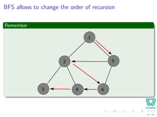
  • 72. BFS allows to change the order of recursion Remember 1 2 3 4 5 6 34 / 84
  • 73. Loop Invariance The While loop This while loop maintains the following invariant : At the test in line 10, the queue Q consists of the set of gray vertices First iteration Q = sand s.color = GRAY Maintenance The inner loop only pushes gray nodes into the queue. 35 / 84
  • 74. Loop Invariance The While loop This while loop maintains the following invariant : At the test in line 10, the queue Q consists of the set of gray vertices First iteration Q = sand s.color = GRAY Maintenance The inner loop only pushes gray nodes into the queue. 35 / 84
  • 75. Loop Invariance The While loop This while loop maintains the following invariant : At the test in line 10, the queue Q consists of the set of gray vertices First iteration Q = sand s.color = GRAY Maintenance The inner loop only pushes gray nodes into the queue. 35 / 84
  • 76. Loop Invariance Termination When every node that can be visited is painted black 36 / 84
  • 77. Example What do you see? 0 0 37 / 84
  • 78. Example What do you see? 0 1 1 1 1 38 / 84
  • 79. Example What do you see? 0 1 2 1 12 39 / 84
  • 80. Example What do you see? 0 2 2 2 1 12 2 2 40 / 84
  • 81. Example What do you see? 0 2 2 1 12 2 2 41 / 84
  • 82. Example What do you see? 0 2 3 1 12 2 2 3 42 / 84
  • 83. Example What do you see? 0 3 3 1 12 2 2 3 3 43 / 84
  • 84. Example What do you see? 0 3 1 12 2 2 3 3 44 / 84
  • 85. Example What do you see? 01 12 2 2 3 3 45 / 84
  • 86. Complexity What about the outer loop? O(V ) Enqueue / Dequeue operations – Each adjacency list is processed only once. What about the inner loop? The sum of the lengths of f all the adjacency lists is Θ(E) so the scanning takes O(E) 46 / 84
  • 87. Complexity What about the outer loop? O(V ) Enqueue / Dequeue operations – Each adjacency list is processed only once. What about the inner loop? The sum of the lengths of f all the adjacency lists is Θ(E) so the scanning takes O(E) 46 / 84
  • 88. Complexity Overhead of Creation O (V ) Then Total complexity O (V + E) 47 / 84
  • 89. Complexity Overhead of Creation O (V ) Then Total complexity O (V + E) 47 / 84
  • 90. Properties: Predecessor Graph Something Notable Breadth-first search constructs a breadth-first tree, initially containing only its root, which is the source vertex s Thus We say that u is the predecessor or parent of v in the breadth-first tree. 48 / 84
  • 91. Properties: Predecessor Graph Something Notable Breadth-first search constructs a breadth-first tree, initially containing only its root, which is the source vertex s Thus We say that u is the predecessor or parent of v in the breadth-first tree. 48 / 84
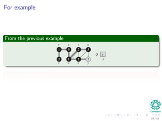
  • 92. For example From the previous example Predecessor Graph 49 / 84
  • 93. For example From the previous example Predecessor Graph s r w v t x yu 49 / 84
  • 94. This allow to use the Algorithm for finding The Shortest Path Clearly This is the unweighted version or all weights are equal!!! We have the following function δ (s, v)= shortest path from s to v We claim that Upon termination of BFS, every vertex v ∈ V reachable from s has v.d = δ(s, v) 50 / 84
  • 95. This allow to use the Algorithm for finding The Shortest Path Clearly This is the unweighted version or all weights are equal!!! We have the following function δ (s, v)= shortest path from s to v We claim that Upon termination of BFS, every vertex v ∈ V reachable from s has v.d = δ(s, v) 50 / 84
  • 96. This allow to use the Algorithm for finding The Shortest Path Clearly This is the unweighted version or all weights are equal!!! We have the following function δ (s, v)= shortest path from s to v We claim that Upon termination of BFS, every vertex v ∈ V reachable from s has v.d = δ(s, v) 50 / 84
  • 97. Intuitive Idea of Claim Correctness of breadth-first search Let G = (V , E) be a directed or undirected graph. Suppose that BFS is run on G from a given source vertex s ∈ V . Then Then, during its execution, BFS discovers every vertex v ∈ V that is reachable from the source. 51 / 84
  • 98. Intuitive Idea of Claim Correctness of breadth-first search Let G = (V , E) be a directed or undirected graph. Suppose that BFS is run on G from a given source vertex s ∈ V . Then Then, during its execution, BFS discovers every vertex v ∈ V that is reachable from the source. 51 / 84
  • 99. Intuitive Idea of Claim Correctness of breadth-first search Let G = (V , E) be a directed or undirected graph. Suppose that BFS is run on G from a given source vertex s ∈ V . Then Then, during its execution, BFS discovers every vertex v ∈ V that is reachable from the source. 51 / 84
  • 100. Intuitive Idea of Claim Distance Idea First, once a node u is reached from v, we use the previous shortest distance from s to update the node distance. 52 / 84
  • 101. Intuitive Idea of Claim You can use the idea of strong induction Given a branch of the breadth-first search u s, u1, u2, ..., un un.π = un−1.π + 1 = un−1.π + 2 = n + s.π = n (2) Thus, we have that For any vertex v = s that is reachable from s, one of the shortest path from s to v is A shortest path from s to v.π followed by thew edge (v.π, v). 53 / 84
  • 102. Intuitive Idea of Claim You can use the idea of strong induction Given a branch of the breadth-first search u s, u1, u2, ..., un un.π = un−1.π + 1 = un−1.π + 2 = n + s.π = n (2) Thus, we have that For any vertex v = s that is reachable from s, one of the shortest path from s to v is A shortest path from s to v.π followed by thew edge (v.π, v). 53 / 84
  • 103. Outline 1 Introduction Graphs Everywhere History Basic Theory Representing Graphs in a Computer 2 Traversing the Graph Breadth-first search Depth-First Search 3 Applications Finding a path between nodes Connected Components Spanning Trees Topological Sorting 54 / 84
  • 104. Depth-first search Given G Pick an unvisited vertex v, remember the rest. Recurse on vertices adjacent to v 55 / 84
  • 105. The Pseudo-code Code for DFS DFS(G) 1. for each vertex u ∈ G.V 2. u.color = WHITE 3. u.π = NIL 4. time = 0 5. for each vertex u ∈ G.V 6. if u.color = WHITE 7. DFS-VISIT(G, u) DFS-VISIT(G, u) 1. time = time + 1 2. u.d = time 3. u.color = GRAY 4. for each vertex v ∈ G.Adj [u] 5. if v.color == WHITE 6. v.π = u 7. DFS-VISIT(G, v) 8. u.color = BLACK 9. time = time + 1 10. u.f = time 56 / 84
  • 106. The Pseudo-code Code for DFS DFS(G) 1. for each vertex u ∈ G.V 2. u.color = WHITE 3. u.π = NIL 4. time = 0 5. for each vertex u ∈ G.V 6. if u.color = WHITE 7. DFS-VISIT(G, u) DFS-VISIT(G, u) 1. time = time + 1 2. u.d = time 3. u.color = GRAY 4. for each vertex v ∈ G.Adj [u] 5. if v.color == WHITE 6. v.π = u 7. DFS-VISIT(G, v) 8. u.color = BLACK 9. time = time + 1 10. u.f = time 56 / 84
  • 107. The Pseudo-code Code for DFS DFS(G) 1. for each vertex u ∈ G.V 2. u.color = WHITE 3. u.π = NIL 4. time = 0 5. for each vertex u ∈ G.V 6. if u.color = WHITE 7. DFS-VISIT(G, u) DFS-VISIT(G, u) 1. time = time + 1 2. u.d = time 3. u.color = GRAY 4. for each vertex v ∈ G.Adj [u] 5. if v.color == WHITE 6. v.π = u 7. DFS-VISIT(G, v) 8. u.color = BLACK 9. time = time + 1 10. u.f = time 56 / 84
  • 108. The Pseudo-code Code for DFS DFS(G) 1. for each vertex u ∈ G.V 2. u.color = WHITE 3. u.π = NIL 4. time = 0 5. for each vertex u ∈ G.V 6. if u.color = WHITE 7. DFS-VISIT(G, u) DFS-VISIT(G, u) 1. time = time + 1 2. u.d = time 3. u.color = GRAY 4. for each vertex v ∈ G.Adj [u] 5. if v.color == WHITE 6. v.π = u 7. DFS-VISIT(G, v) 8. u.color = BLACK 9. time = time + 1 10. u.f = time 56 / 84
  • 109. The Pseudo-code Code for DFS DFS(G) 1. for each vertex u ∈ G.V 2. u.color = WHITE 3. u.π = NIL 4. time = 0 5. for each vertex u ∈ G.V 6. if u.color = WHITE 7. DFS-VISIT(G, u) DFS-VISIT(G, u) 1. time = time + 1 2. u.d = time 3. u.color = GRAY 4. for each vertex v ∈ G.Adj [u] 5. if v.color == WHITE 6. v.π = u 7. DFS-VISIT(G, v) 8. u.color = BLACK 9. time = time + 1 10. u.f = time 56 / 84
  • 110. The Pseudo-code Code for DFS DFS(G) 1. for each vertex u ∈ G.V 2. u.color = WHITE 3. u.π = NIL 4. time = 0 5. for each vertex u ∈ G.V 6. if u.color = WHITE 7. DFS-VISIT(G, u) DFS-VISIT(G, u) 1. time = time + 1 2. u.d = time 3. u.color = GRAY 4. for each vertex v ∈ G.Adj [u] 5. if v.color == WHITE 6. v.π = u 7. DFS-VISIT(G, v) 8. u.color = BLACK 9. time = time + 1 10. u.f = time 56 / 84
  • 111. The Pseudo-code Code for DFS DFS(G) 1. for each vertex u ∈ G.V 2. u.color = WHITE 3. u.π = NIL 4. time = 0 5. for each vertex u ∈ G.V 6. if u.color = WHITE 7. DFS-VISIT(G, u) DFS-VISIT(G, u) 1. time = time + 1 2. u.d = time 3. u.color = GRAY 4. for each vertex v ∈ G.Adj [u] 5. if v.color == WHITE 6. v.π = u 7. DFS-VISIT(G, v) 8. u.color = BLACK 9. time = time + 1 10. u.f = time 56 / 84
  • 112. Example What do we do? 57 / 84
  • 113. Example What do we do? 58 / 84
  • 114. Example What do we do? 59 / 84
  • 115. Example What do we do? 60 / 84
  • 116. Example What do we do? 61 / 84
  • 117. Example What do we do? 62 / 84
  • 118. Example What do we do? 63 / 84
  • 119. Example What do we do? 64 / 84
  • 120. Complexity Analysis 1 The loops on lines 1–3 and lines 5–7 of DFS take Θ (V ). 2 The procedure DFS-VISIT is called exactly once for each vertex v ∈ V . 3 During an execution of DFS-VISIT(G, v) the loop on lines 4–7 executes |Adj (v)| times. 4 But v∈V |Adj (v)| = Θ (E) we have that the cost of executing g lines 4–7 of DFS-VISIT is Θ (E) . Then DFS complexity is Θ (V + E) 65 / 84
  • 121. Complexity Analysis 1 The loops on lines 1–3 and lines 5–7 of DFS take Θ (V ). 2 The procedure DFS-VISIT is called exactly once for each vertex v ∈ V . 3 During an execution of DFS-VISIT(G, v) the loop on lines 4–7 executes |Adj (v)| times. 4 But v∈V |Adj (v)| = Θ (E) we have that the cost of executing g lines 4–7 of DFS-VISIT is Θ (E) . Then DFS complexity is Θ (V + E) 65 / 84
  • 122. Complexity Analysis 1 The loops on lines 1–3 and lines 5–7 of DFS take Θ (V ). 2 The procedure DFS-VISIT is called exactly once for each vertex v ∈ V . 3 During an execution of DFS-VISIT(G, v) the loop on lines 4–7 executes |Adj (v)| times. 4 But v∈V |Adj (v)| = Θ (E) we have that the cost of executing g lines 4–7 of DFS-VISIT is Θ (E) . Then DFS complexity is Θ (V + E) 65 / 84
  • 123. Complexity Analysis 1 The loops on lines 1–3 and lines 5–7 of DFS take Θ (V ). 2 The procedure DFS-VISIT is called exactly once for each vertex v ∈ V . 3 During an execution of DFS-VISIT(G, v) the loop on lines 4–7 executes |Adj (v)| times. 4 But v∈V |Adj (v)| = Θ (E) we have that the cost of executing g lines 4–7 of DFS-VISIT is Θ (E) . Then DFS complexity is Θ (V + E) 65 / 84
  • 124. Complexity Analysis 1 The loops on lines 1–3 and lines 5–7 of DFS take Θ (V ). 2 The procedure DFS-VISIT is called exactly once for each vertex v ∈ V . 3 During an execution of DFS-VISIT(G, v) the loop on lines 4–7 executes |Adj (v)| times. 4 But v∈V |Adj (v)| = Θ (E) we have that the cost of executing g lines 4–7 of DFS-VISIT is Θ (E) . Then DFS complexity is Θ (V + E) 65 / 84
  • 125. Applications We have several Topological Sort Strongly Connected Components Computer Vision Algorithms Artificial Intelligence Algorithms Importance in Social Network Rank Algorithms for Google Etc. 66 / 84
  • 126. Applications We have several Topological Sort Strongly Connected Components Computer Vision Algorithms Artificial Intelligence Algorithms Importance in Social Network Rank Algorithms for Google Etc. 66 / 84
  • 127. Applications We have several Topological Sort Strongly Connected Components Computer Vision Algorithms Artificial Intelligence Algorithms Importance in Social Network Rank Algorithms for Google Etc. 66 / 84
  • 128. Applications We have several Topological Sort Strongly Connected Components Computer Vision Algorithms Artificial Intelligence Algorithms Importance in Social Network Rank Algorithms for Google Etc. 66 / 84
  • 129. Applications We have several Topological Sort Strongly Connected Components Computer Vision Algorithms Artificial Intelligence Algorithms Importance in Social Network Rank Algorithms for Google Etc. 66 / 84
  • 130. Applications We have several Topological Sort Strongly Connected Components Computer Vision Algorithms Artificial Intelligence Algorithms Importance in Social Network Rank Algorithms for Google Etc. 66 / 84
  • 131. Applications We have several Topological Sort Strongly Connected Components Computer Vision Algorithms Artificial Intelligence Algorithms Importance in Social Network Rank Algorithms for Google Etc. 66 / 84
  • 132. Outline 1 Introduction Graphs Everywhere History Basic Theory Representing Graphs in a Computer 2 Traversing the Graph Breadth-first search Depth-First Search 3 Applications Finding a path between nodes Connected Components Spanning Trees Topological Sorting 67 / 84
  • 133. Finding a path between nodes We do the following Start a breadth-first search at vertex v. Terminate when vertex u is visited or when Q becomes empty (whichever occurs first). Time Complexity O V 2 when adjacency matrix used. O(V + E) when adjacency lists used. 68 / 84
  • 134. Finding a path between nodes We do the following Start a breadth-first search at vertex v. Terminate when vertex u is visited or when Q becomes empty (whichever occurs first). Time Complexity O V 2 when adjacency matrix used. O(V + E) when adjacency lists used. 68 / 84
  • 135. Finding a path between nodes We do the following Start a breadth-first search at vertex v. Terminate when vertex u is visited or when Q becomes empty (whichever occurs first). Time Complexity O V 2 when adjacency matrix used. O(V + E) when adjacency lists used. 68 / 84
  • 136. Finding a path between nodes We do the following Start a breadth-first search at vertex v. Terminate when vertex u is visited or when Q becomes empty (whichever occurs first). Time Complexity O V 2 when adjacency matrix used. O(V + E) when adjacency lists used. 68 / 84
  • 137. This allow to use the Algorithm for finding The Shortest Path Clearly This is the unweighted version or all weights are equal!!! We have the following function δ (s, v)= shortest path from s to v Actually Upon termination of BFS, every vertex v ∈ V reachable from s has distance(v) = δ(s, v) 69 / 84
  • 138. This allow to use the Algorithm for finding The Shortest Path Clearly This is the unweighted version or all weights are equal!!! We have the following function δ (s, v)= shortest path from s to v Actually Upon termination of BFS, every vertex v ∈ V reachable from s has distance(v) = δ(s, v) 69 / 84
  • 139. This allow to use the Algorithm for finding The Shortest Path Clearly This is the unweighted version or all weights are equal!!! We have the following function δ (s, v)= shortest path from s to v Actually Upon termination of BFS, every vertex v ∈ V reachable from s has distance(v) = δ(s, v) 69 / 84
  • 140. Outline 1 Introduction Graphs Everywhere History Basic Theory Representing Graphs in a Computer 2 Traversing the Graph Breadth-first search Depth-First Search 3 Applications Finding a path between nodes Connected Components Spanning Trees Topological Sorting 70 / 84
  • 141. Connected Components Definition A connected component (or just component) of an undirected graph is a subgraph in which any two vertices are connected to each other by paths. Example 71 / 84
  • 142. Connected Components Definition A connected component (or just component) of an undirected graph is a subgraph in which any two vertices are connected to each other by paths. Example 71 / 84
  • 143. Procedure First Start a breadth-first search at any as yet unvisited vertex of the graph. Thus Newly visited vertices (plus edges between them) define a component. Repeat Repeat until all vertices are visited. 72 / 84
  • 144. Procedure First Start a breadth-first search at any as yet unvisited vertex of the graph. Thus Newly visited vertices (plus edges between them) define a component. Repeat Repeat until all vertices are visited. 72 / 84
  • 145. Procedure First Start a breadth-first search at any as yet unvisited vertex of the graph. Thus Newly visited vertices (plus edges between them) define a component. Repeat Repeat until all vertices are visited. 72 / 84
  • 146. Time O (V 2 ) When adjacency matrix used O(V + E) When adjacency lists used (E is number of edges) 73 / 84
  • 147. Time O (V 2 ) When adjacency matrix used O(V + E) When adjacency lists used (E is number of edges) 73 / 84
  • 148. Outline 1 Introduction Graphs Everywhere History Basic Theory Representing Graphs in a Computer 2 Traversing the Graph Breadth-first search Depth-First Search 3 Applications Finding a path between nodes Connected Components Spanning Trees Topological Sorting 74 / 84
  • 149. Spanning Tree with edges with same weight of no weight Definition A spanning tree of a graph G = (V , E) is a acyclic graph where for u, v ∈ V , there is a path between them Example 75 / 84
  • 150. Spanning Tree with edges with same weight of no weight Definition A spanning tree of a graph G = (V , E) is a acyclic graph where for u, v ∈ V , there is a path between them Example 2 3 5 1 4 6 7 9 8 75 / 84
  • 151. Procedure First Start a breadth-first search at any vertex of the graph. Thus If graph is connected, the n − 1 edges used to get to unvisited vertices define a spanning tree (breadth-first spanning tree). 76 / 84
  • 152. Procedure First Start a breadth-first search at any vertex of the graph. Thus If graph is connected, the n − 1 edges used to get to unvisited vertices define a spanning tree (breadth-first spanning tree). 76 / 84
  • 153. Time O (V 2 ) When adjacency matrix used O(V + E) When adjacency lists used (E is number of edges) 77 / 84
  • 154. Time O (V 2 ) When adjacency matrix used O(V + E) When adjacency lists used (E is number of edges) 77 / 84
  • 155. Outline 1 Introduction Graphs Everywhere History Basic Theory Representing Graphs in a Computer 2 Traversing the Graph Breadth-first search Depth-First Search 3 Applications Finding a path between nodes Connected Components Spanning Trees Topological Sorting 78 / 84
  • 156. Topological Sorting Definitions A topological sort (sometimes abbreviated topsort or toposort) or topological ordering of a directed graph is a linear ordering of its vertices such that for every directed edge (u, v) from vertex u to vertex y, u comes before v in the ordering. From Industrial Engineering The canonical application of topological sorting (topological order) is in scheduling a sequence of jobs or tasks based on their dependencies. Topological sorting algorithms were first studied in the early 1960s in the context of the PERT technique for scheduling in project management (Jarnagin 1960). 79 / 84
  • 157. Topological Sorting Definitions A topological sort (sometimes abbreviated topsort or toposort) or topological ordering of a directed graph is a linear ordering of its vertices such that for every directed edge (u, v) from vertex u to vertex y, u comes before v in the ordering. From Industrial Engineering The canonical application of topological sorting (topological order) is in scheduling a sequence of jobs or tasks based on their dependencies. Topological sorting algorithms were first studied in the early 1960s in the context of the PERT technique for scheduling in project management (Jarnagin 1960). 79 / 84
  • 158. Then We have that The jobs are represented by vertices, and there is an edge from x to y if job x must be completed before job y can be started. Example When washing clothes, the washing machine must finish before we put the clothes to dry. Then A topological sort gives an order in which to perform the jobs. 80 / 84
  • 159. Then We have that The jobs are represented by vertices, and there is an edge from x to y if job x must be completed before job y can be started. Example When washing clothes, the washing machine must finish before we put the clothes to dry. Then A topological sort gives an order in which to perform the jobs. 80 / 84
  • 160. Then We have that The jobs are represented by vertices, and there is an edge from x to y if job x must be completed before job y can be started. Example When washing clothes, the washing machine must finish before we put the clothes to dry. Then A topological sort gives an order in which to perform the jobs. 80 / 84
  • 161. Algorithm Pseudo Code TOPOLOGICAL-SORT 1 Call DFS(G) to compute finishing times v.f for each vertex v. 2 As each vertex is finished, insert it onto the front of a linked list 3 Return the linked list of vertices 81 / 84
  • 162. Algorithm Pseudo Code TOPOLOGICAL-SORT 1 Call DFS(G) to compute finishing times v.f for each vertex v. 2 As each vertex is finished, insert it onto the front of a linked list 3 Return the linked list of vertices 81 / 84
  • 163. Algorithm Pseudo Code TOPOLOGICAL-SORT 1 Call DFS(G) to compute finishing times v.f for each vertex v. 2 As each vertex is finished, insert it onto the front of a linked list 3 Return the linked list of vertices 81 / 84
  • 165. Thus Using the u.f As each vertex is finished, insert it onto the front of a linked list 83 / 84
  • 166. Example After Sorting undershortsocks pants beltshirt tie jacketshoes watch 11/16 12/15 6/71/8 2/5 3/417/18 13/14 9/10 84 / 84