3. What is classification?
A machine learning task that deals with identifying the class to which
an instance belongs
A classifier performs classification
Classifier
Test instance
Attributes
(a1, a2,… an)
Discrete-valued
Class label
( Age, Marital status,
Health status, Salary ) Issue Loan? {Yes, No}
( Perceptive inputs )
Steer? { Left, Straight,
Right }
Category of document?
{Politics, Movies,
Biology}
( Textual features :
Ngrams )
7. Generating datasets
• Methods:
– Holdout (2/3rd
training, 1/3rd
testing)
– Cross validation (n – fold)
• Divide into n parts
• Train on (n-1), test on last
• Repeat for different combinations
– Bootstrapping
• Select random samples to form the training set
9. Types of Learners in Classification
Lazy learners
simply store the
training data
and wait until a
testing data
appears
Eager learners
construct a
classification
model based on
the given
training data
before getting
data for
prediction
Lazy
Learners
Eager
Learners
10. Classification Algorithms
• Logistic Regression
• Decision Tree
• K-nearest Neighbor
• Support Vector Machine
• Artificial Neural Network
• Naïve Bayes
• Random Forest
• Stochastic Gradient Descent
11. Evaluating classifiers
• Outcome:
– Accuracy
– Confusion matrix
– If cost-sensitive, the expected cost of
classification ( attribute test cost +
misclassification cost)
etc.
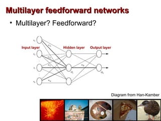
13. Diagram from Han-Kamber
Example tree
Intermediate nodes : Attributes
Leaf nodes : Class predictions
Edges : Attribute value tests
Example algorithms: ID3, C4.5, SPRINT, CART
14. Decision Tree schematic
Training data set
a1 a2 a3 a4 a5 a6
a1 a2 a3 a4 a5 a6
X Y Z
Pure node,
Leaf node:
Class RED
Impure node,
Select best attribute
and continue
Impure node,
Select best attribute
and continue
15. Decision Tree Issues
How to avoid overfitting?
Problem: Classifier performs well on training data, but fails
to give good results on test data
Example: Split on primary key gives pure nodes and good
accuracy on training – not for testing
Alternatives:
1. Pre-prune : Halting construction at a certain level of tree /
level of purity
2. Post-prune : Remove a node if the error rate remains
the same without it. Repeat process for all nodes in the d.tree
How does the type of attribute affect the split?
• Discrete-valued: Each branch corresponding to a value
• Continuous-valued: Each branch may be a range of values
(e.g.: splits may be age < 30, 30 < age < 50, age > 50 )
(aimed at maximizing the gain/gain ratio)
How to determine the attribute for split?
Alternatives:
1. Information Gain
Gain (A, S) = Entropy (S) – Σ ( (Sj/S)*Entropy(Sj) )
Other options:
Gain ratio, etc.
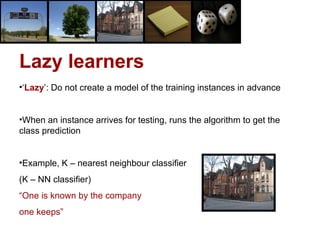
17. Lazy learners
•‘Lazy’: Do not create a model of the training instances in advance
•When an instance arrives for testing, runs the algorithm to get the
class prediction
•Example, K – nearest neighbour classifier
(K – NN classifier)
“One is known by the company
one keeps”
18. K-NN classifier schematic
For a test instance,
1) Calculate distances from training pts.
2) Find K-nearest neighbours (say, K = 3)
3) Assign class label based on majority
19. How good is it?
• Susceptible to noisy values
• Slow because of distance calculation
Alternate approaches:
• Distances to representative points only
• Partial distance
Any other modifications?
Alternatives:
1. Weighted attributes to decide final label
2. Assign distance to missing values as <max>
3. K=1 returns class label of nearest neighbour
How to determine value of K?
Alternatives:
1. Determine K experimentally. The K that gives minimum
error is selected.
K-NN classifier Issues
How to make real-valued prediction?
Alternative:
1. Average the values returned by K-nearest neighbours
How to determine distances between values of categorical
attributes?
Alternatives:
1. Boolean distance (1 if same, 0 if different)
2. Differential grading (e.g. weather – ‘drizzling’ and ‘rainy’ are
closer than ‘rainy’ and ‘sunny’ )
21. • A sequence of boolean functions that lead
to a result
• if h1 (y) = 1 then set f (y) = c1
else if h2 (y) = 1 then set f (y) = c2
…. else set f (y) = cn
Decision Lists
Decision Lists
f ( y ) = cj, if j = min { i | hi (y) = 1 } exists
0 otherwise
23. Decision List learning
Decision List learning
R S’ = S
Set of candidate
feature functions
For each hi,
Qi = Pi U Ni
( hi = 1 )
U i = max { | Pi| - pn * | Ni | , |Ni| - pp *|Pi| }
Select hk, the feature
with
highest utility
( h k, )
If
(| Pi| - pn * | Ni |
>
|Ni| - pp *|Pi| )
then 1
else 0
1 / 0
- Qk
24. Pruning?
hi is not required if :
1.c i = c (r+1)
2.There is no h j ( j > i ) such that
Q i = Q j
Decision list Issues
Accuracy / Complexity tradeoff?
Size of R : Complexity (Length of the list)
S’ contains examples of both classes : Accuracy (Purity)
What is the terminating condition?
1. Size of R (an upper threshold)
2. Qk = null
3. S’ contains examples of same class
26. Probabilistic classifiers : NB
Probabilistic classifiers : NB
• Based on Bayes rule
• Naïve Bayes : Conditional independence
assumption
27. How are different types of attributes
handled?
1. Discrete-valued : P ( X | Ci ) is according to
formula
2. Continous-valued : Assume gaussian distribution.
Plug in mean and variance for the attribute
and assign it to P ( X | Ci )
Naïve Bayes Issues
Problems due to sparsity of data?
Problem : Probabilities for some values may be zero
Solution : Laplace smoothing
For each attribute value,
update probability m / n as : (m + 1) / (n + k)
where k = domain of values
28. Probabilistic classifiers : BBN
Probabilistic classifiers : BBN
• Bayesian belief networks : Attributes ARE
dependent
• A directed acyclic graph and conditional
probability tables
Diagram from Han-Kamber
An added term for conditional
probability between attributes:
29. BBN learning
BBN learning
(when network structure known)
(when network structure known)
• Input : Network topology of BBN
• Output : Calculate the entries in conditional
probability table
(when network structure not known)
(when network structure not known)
• ???
???
30. Learning structure of BBN
Learning structure of BBN
• Use Naïve Bayes as a basis pattern
• Add edges as required
• Examples of algorithms: TAN, K2
Loan
Age
Family
status
Marital
status
32. Artificial Neural Networks
Artificial Neural Networks
• Based on biological concept of neurons
• Structure of a fundamental unit of ANN:
w0
w1
wn
threshold
output: : activation function
p (v) where
p (v) = sgn (w0 + w1x1 + …
+ wnxn )
input
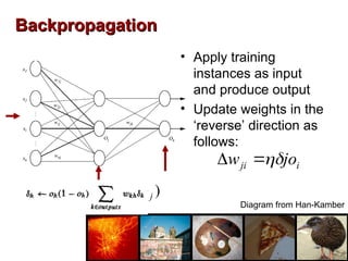
33. Perceptron learning algorithm
Perceptron learning algorithm
• Initialize values of weights
• Apply training instances and get output
• Update weights according to the update rule:
• Repeat till converges
• Can represent linearly separable functions only
n : learning rate
t : target output
o : observed output
37. Addition of momentum
But why?
Choosing the learning factor
A small learning factor means multiple iterations
required.
A large learning factor means the learner
may skip the global minimum
ANN Issues
What are the types of learning
approaches?
Deterministic: Update weights after summing up
Errors over all examples
Stochastic: Update weights per example
Learning the structure of the network
1. Construct a complete network
2. Prune using heuristics:
• Remove edges with weights nearly zero
• Remove edges if the removal does not affect
accuracy
39. Support vector machines
Support vector machines
• Basic ideas
Separating hyperplane : wx+b = 0
Margin
Support vectors
“Maximum separating-
margin classifier”
+1
-1
40. SVM training
SVM training
• Problem formulation
Minimize (1 / 2) || w ||2
w.r.t. (yi ( w xi + b ) – 1) >= 0 for all iLagrangian multipliers are
zero for data instances other
than support vectors
Dot product of xk and xl
41. Focussing on dot product
Focussing on dot product
• For non-linear separable points,
we plan to map them to a higher dimensional (and linearly
separable) space
• The product can be time-consuming.
Therefore, we use kernel functions
42. Kernel functions
Kernel functions
• Without having to know the non-linear mapping, apply
kernel function, say,
• Reduces the number of computations required to generate
Q kl values.
44. SVMs are immune to the removal of
non-support-vector points
SVM Issues
What if n-classes are to be predicted?
Problem : SVMs deal with two-class classification
Solution : Have multiple SVMs each for one class
46. Combining Classifiers
Combining Classifiers
• ‘Ensemble’ learning
• Use a combination of models for prediction
– Bagging : Majority votes
– Boosting : Attention to the ‘weak’ instances
• Goal : An improved combined model
48. Total set
Boosting (AdaBoost)
Boosting (AdaBoost)
Sample
D 1
Classifier
model
M 1
Selection based on weight. May use
bootstrap sampling with replacement
Training
dataset
D
Classifier
learning
scheme
Classifier
model
M n
Test
set
Weighted
vote Class Label
Initialize weights of instances to 1/d
Weights of
correctly classified
instances multiplied
by error / (1 – error)
If error > 0.5?
Error
Error
`
50. Data preprocessing
• Attribute subset selection
– Select a subset of total attributes to reduce
complexity
• Dimensionality reduction
– Transform instances into ‘smaller’ instances
51. Attribute subset selection
• Information gain measure for attribute
selection in decision trees
• Stepwise forward / backward elimination of
attributes
52. Dimensionality reduction
• High dimensions : Computational
complexity
Number of attributes of
a data instance
instance x in
p-dimensions
instance x in
k-dimensions
k < p
s = Wx W is k x p transformation mtrx.
53. Principal Component Analysis
• Computes k orthonormal vectors :
Principal components
• Essentially provide a new set of axes – in
decreasing order of variance
Eigenvector matrix
( p X p )
First k are k PCs
( p X n )
( p X n )
(k X n)
(p X n)
(k X p) Diagram from Han-Kamber
55. Weka & Weka Demo
Weka & Weka Demo
• Collection of ML algorithms
Collection of ML algorithms
• Get it from :
Get it from :
http://www.cs.waikato.ac.nz/ml/weka/
• ARFF Format
ARFF Format
• ‘
‘Weka Explorer’
Weka Explorer’
56. ARFF file format
ARFF file format
@RELATION nursery
@RELATION nursery
@ATTRIBUTE children numeric
@ATTRIBUTE children numeric
@ATTRIBUTE housing {convenient, less_conv, critical}
@ATTRIBUTE housing {convenient, less_conv, critical}
@ATTRIBUTE finance {convenient, inconv}
@ATTRIBUTE finance {convenient, inconv}
@ATTRIBUTE social {nonprob, slightly_prob, problematic}
@ATTRIBUTE social {nonprob, slightly_prob, problematic}
@ATTRIBUTE health {recommended, priority, not_recom}
@ATTRIBUTE health {recommended, priority, not_recom}
@ATTRIBUTE pr_val
@ATTRIBUTE pr_val
{recommend,priority,not_recom,very_recom,spec_prior}
{recommend,priority,not_recom,very_recom,spec_prior}
@DATA
@DATA
3,less_conv,convenient,slightly_prob,recommended,spec_prior
3,less_conv,convenient,slightly_prob,recommended,spec_prior
Name of the relation
Attribute definition
Data instances : Comma separated, each on a new line
57. Parts of weka
Parts of weka
Explorer
Basic interface to run ML
Algorithms
Experimenter
Comparing experiments
on different algorithms
Knowledge Flow
Similar to Work Flow
‘Customized’ to one’s needs
59. Key Sources of Lecture
• Data Mining – Concepts and techniques; Han and
Kamber, Morgan Kaufmann publishers, 2006.
• Machine Learning; Tom Mitchell, McGraw Hill
publications.
• Data Mining – Practical machine learning tools and
techniques; Witten and Frank, Morgan Kaufmann
publishers, 2005.
60. Extra slides 1
Difference between decision lists and decision trees:
1. Lists are functions tested sequentially (More than one
attributes at a time)
Trees are attributes tested sequentially
2. Lists may not require a ‘complete’ coverage for values
of an attribute.
All values of an attribute correspond to atleast one
branch of the attribute split.
61. Learning structure of BBN
Learning structure of BBN
• K2 Algorithm :
– Consider nodes in an order
– For each node, calculate utility to add an edge from
previous nodes to this one
• TAN :
– Use Naïve Bayes as the baseline network
– Add different edges to the network based on utility
• Examples of algorithms: TAN, K2
62. Delta rule
Delta rule
• Delta rule enables to converge to a best fit
if points are not linearly separable
• Uses gradient descent to choose the
hypothesis space