


![a
m
p
l
e
v
a
r
1
=
'
P
y
t
h
o
n'
p
ri
n
t
(
v
a
r
1
*
3
)
# PythonPythonPython
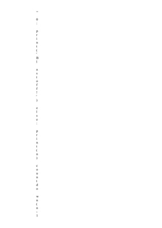
Slicing [ ]:The slice operator prints the character at a given index.
#
examp
le
var1
=
'Pytho
n'
print (var1[2]) # t
Range Slicing [x:y]
It prints the characters present in the given range.
#
example
var1 =
'Python'
print
(var1[2:
5]) # tho
Membership (in):This operator returns ‘True’ value if the character is present in the given
String.](https://image.slidesharecdn.com/aintroductionbookofpythonforbeginners-250613145832-83400372/85/A-Introduction-Book-of-python-For-Beginners-docx-9-320.jpg)


![EXAMPLE1:
var1 = 'Hello
World!' var2 =
"Python
Programming"
print "var1[0]: ",
var1[0] print
"var2[1:5]: ",
var2[1:5]
When the above code is executed, it produces the following
result − var1[0]: H
var2[1:5]: ytho
EXAMPLE2:
var1 = 'Hello World!'
print "Updated String :- ", var1[:6] +
'Python'
When the above code is executed, it produces the following
result − Updated String :- Hello Python
5. Comments:
Comments are of two types .
Single-line comments
Multi line Comments
Single-line comments are created simply by beginning a line with the hash
(#) character, and they are automatically terminated by the end of line. For
Ex: #This would be a comment in Python
Multi Line Comments that span multiple lines and are created by adding a
delimiter (“””) on each end of the comment For Ex:
"""
This would be a multiline comment in Python that spans several lines and describes
your code, your day, or anything you want it to """
Chapter-3 Functions
What is a Function in Python?
A Function in Python is used to utilize the code in more than one place in a
program. It is also called method or procedures. Python provides you many
inbuilt functions like print(), but it also gives freedom to create your own
functions.
Functions:
A function is a named sequence of statements that performs a computation.
How to define and call a function in Python
Function in Python is defined by the "def " statement followed by the
function name and parentheses ( () ) Example:](https://image.slidesharecdn.com/aintroductionbookofpythonforbeginners-250613145832-83400372/85/A-Introduction-Book-of-python-For-Beginners-docx-15-320.jpg)

![Arguments in Functions
The argument is a value that is passed to the function when it's called.In other words on
the calling side, it is an argument and on the function side it is a parameter. Let see how
Python Args works - Step 1) Arguments are declared in the function definition. While
calling the function, you can pass the values for that args as shown below
Step 2) To declare a default value of an argument, assign it a value at function definition.
Example: x has no default values. Default values of y=0. When we supply only
one argument while calling multiply function, Python assigns the supplied value
to x while keeping the value of y=0. Hence the multiply of x*y=0
Step 3) This time we will change the value to y=2 instead of the default value y=0,
and it will return the output as (4x2)=8.
Step 4) You can also change the order in which the arguments can be passed in
Python. Here we have reversed the order of the value x and y to x=4 and y=2.
Step 5) Multiple Arguments can also be passed as an array. Here in the example
we call the multiple args (1,2,3,4,5) by calling the (*args) function.
Example: We declared multiple args as number (1,2,3,4,5) when we call the
(*args) function; it prints out the output as (1,2,3,4,5)
Rules to define a function in Python.
Function blocks begin with the keyword def followed by the function name and
parentheses ( ( ) ).Any input parameters or arguments should be placed within
these parentheses. You can also define parameters inside these parentheses.The
code block within every function starts with a colon (:) and is indented. The
statement return [expression] exits a function, but it is optional
Syntax:
def functionname( parameters ):
functio
n_suite
return
[expres
sion]
Creati
ng a
Functi
on
In Python a function is defined using the
def keyword: Example def
my_function():
print("Hello from a function")
Calling a Function
To call a function, use the function name followed
by parenthesis: Example def my_function():
print("Hello from a function")
my_function() #calling function](https://image.slidesharecdn.com/aintroductionbookofpythonforbeginners-250613145832-83400372/85/A-Introduction-Book-of-python-For-Beginners-docx-17-320.jpg)

![4 inf - Returns the infinite
5 nan - Not a number type.
Numbers and Numeric Representation
These functions are used to represent numbers in different forms. The methods are
like below −
Sr.No. Function & Description
1 ceil(x)
Return the Ceiling value. It is the smallest integer, greater or equal to the number
x.
3 fabs(x)
Returns the absolute value of x.
4 factorial(x)
Returns factorial of x. where x ≥ 0
5 floor(x)
Return the Floor value. It is the largest integer, less or equal to the number x.
6 fsum(iterable)
Find sum of the elements in an iterable object
7 gcd(x, y)
Returns the Greatest Common Divisor of x and y
8 isfinite(x)
Checks whether x is neither an infinity nor nan.
9 isinf(x)
Checks whether x is infinity
10 isnan(x)
Checks whether x is not a number.
11 remainder(x, y)
Find remainder after dividing x by y
Example program:
import math
print(math.ceil(23.56) )
my_list = [12, 4.25, 89, 3.02, -65.23, -7.2, 6.3]
print(math.fsum(my_list))
print('The GCD of 24 and 56 : ' +
str(math.gcd(24, 56))) x = float('nan') if
math.isnan(x):
print('It is not a number')](https://image.slidesharecdn.com/aintroductionbookofpythonforbeginners-250613145832-83400372/85/A-Introduction-Book-of-python-For-Beginners-docx-19-320.jpg)
![x =
float('i
nf')
y = 45
if
math.i
sinf(x)
:
print('
It is
Infinit
y')
print(math.isfinite(x)) #x is not a finite number
print(math.isfinite(y)) #y is a finite number
O/P:
24
42.13999999999999
The GCD of 24 and 56 : 8
It is not a number
It is Infinity
False
True
>>>
Power and Logarithmic Functions
These functions are used to calculate different power related and logarithmic related
tasks.
Sr.No. Function & Description
1 pow(x, y)
Return the x to the power y value.
2 sqrt(x)
Finds the square root of x
3 exp(x)
Finds xe, where e = 2.718281
4 log(x[, base])
Returns the Log of x, where base is given. The default base is e
5 log2(x)
Returns the Log of x, where base is 2
6 log10(x)
Returns the Log of x, where base is 10
Example
Code
import
math](https://image.slidesharecdn.com/aintroductionbookofpythonforbeginners-250613145832-83400372/85/A-Introduction-Book-of-python-For-Beginners-docx-20-320.jpg)

![The value of cos(pi): -1.0
The value of tan(90 degree): 1.633123935319537e+16
The angle of sin(0.8660254037844386): 59.99999999999999
3. Composition:
So far, we have looked at the elements of a program—variables, expressions, and
statements—in isolation, without talking about how to combine(Composition)
them.For example, the argument of a function can be any kind of expression, including
arithmetic operators: x = math.sin(degrees / 360.0 * 2 * math.pi) And even function
calls:
x = math.exp(math.log(x+1))
4. Adding new functions:
Pass by reference vs value:All parameters (arguments) in the Python language are passed by
reference. It means if you change what a parameter refers to within a function, the change also
reflects back in the calling function. For example −
#!/usr/bin/python
# Function
definition is here
def changeme(
mylist ):
"This changes a passed list into this
function" mylist.append([1,2,3,4]);
print "Values inside the function: ",
mylist return
# Now you can call changeme function
mylist =
[10,20,30];
changeme( mylist
);
print "Values outside the function: ",
mylist
Here, we are maintaining reference of the passed object and appending
values in the same object. So, this would produce the following result −
Values inside the function: [10, 20, 30, [1, 2, 3, 4]]
Values outside the function: [10, 20, 30, [1, 2, 3, 4]]
Scope of Variables:All variables in a program may not be accessible at all
locations in that program. This depends on where you have declared a
variable.The scope of a variable determines the portion of the program where
you can access a particular identifier. There are two basic scopes of variables
in Python −
Global
variables
Local
variables
Global vs. Local variables:Variables that are defined inside a function body have a
local scope, and those defined outside have a global scope.This means that local
variables can be accessed only inside the function in which they are declared,](https://image.slidesharecdn.com/aintroductionbookofpythonforbeginners-250613145832-83400372/85/A-Introduction-Book-of-python-For-Beginners-docx-22-320.jpg)
![whereas global variables can be accessed throughout the program body by all
functions. When you call a function, the variables declared inside it are brought into
scope. Following is a simple example −
#!/usr/bin/python
total = 0; # This is
global variable. #
Function definition is
here def sum( arg1,
arg2 ):
# Add both the parameters and
return them." total = arg1 + arg2; #
Here total is local variable. print
"Inside the function local total : ",
total return total;
# Now you can call sum function
sum( 10, 20 );
print "Outside the function global
total : ", total
When the above code is executed, it produces the following result −
Inside the function local total : 30
Outside the function global total : 0
The import Statement
You can use any Python source file as a module by executing an import statement in
some other Python source file. The import has the following syntax −
import module1[, module2[,... moduleN]
When the interpreter encounters an import statement, it imports the module if
the module is present in the search path. A search path is a list of directories that
the interpreter searches before importing a module. For example, to import the
module support.py, you need to put the following command at the top of the
script − #!/usr/bin/python
# Import module
support import
support
# Now you can call defined function that module as follows
support.print_func("Zara")
When the above code is executed, it produces the following
result − Hello : Zara
5. Flow of Execution
The order in which statements are executed is called the
flow of execution Execution always begins at the first
statement of the program.
Statements are executed one at a time, in order, from top to
bottom.
Function definitions do not alter the flow of execution of the program, but
remember that statements inside the function are not executed until the function
is called.](https://image.slidesharecdn.com/aintroductionbookofpythonforbeginners-250613145832-83400372/85/A-Introduction-Book-of-python-For-Beginners-docx-23-320.jpg)


![# Now you can call printinfo
function printinfo( age=50,
name="miki" ) printinfo(
name="miki" )
When the above code is executed, it produces the following
result − Name: miki
Age 50
Name: miki
Age 35
Variable-length arguments
You may need to process a function for more arguments than you specified
while defining the function. These arguments are called variable-length
arguments and are not named in the function definition, unlike required and
default arguments.Syntax for a function with non- keyword variable arguments
is this − def functionname([formal_args,] *var_args_tuple ):
"functi
on_doc
string"
functio
n_suite
return
[expres
sion]
An asterisk (*) is placed before the variable name that holds the values of all
nonkeyword variable arguments. This tuple remains empty if no additional
arguments are specified during the function call. Following is a simple example
−
#!/usr/bin/python
# Function
definition is here
def printinfo(
arg1, *vartuple ):
"This prints a variable passed
arguments"
print
"Out
put
is: "
print
arg1
for
var in
vartu
ple:
print
var
retur
n;
# Now you can call printinfo function](https://image.slidesharecdn.com/aintroductionbookofpythonforbeginners-250613145832-83400372/85/A-Introduction-Book-of-python-For-Beginners-docx-26-320.jpg)
![printinfo(
10 )
printinfo(
70, 60, 50
)
When the above code is executed, it produces the following
result − Output is:
10
Output is:
70
60
50
Example
def
my_functio
n(fname):
print(fname + " krishna") my_function("Rama") my_function("Siva")
my_function("Hari") o/p: Ramakrishna Sivakrishna
Harikrishna.
Parameters Vs Arguments
A parameter is the variable listed inside the parentheses in the function
definition. An argument is the value that is sent to the function when it
is called.
Number of Arguments
A function must be called with the correct number of arguments. Meaning that if
your function expects 2 arguments, you have to call the function with 2
arguments, not more, and not less.
Example
This function expects 2 arguments, and gets 2 arguments:
def my_function(fname, lname):
print(fname + " " + lname)
my_function("Srinu", "vasulu")
Arbitrary Arguments( *args)
If you do not know how many arguments that will be passed into your
function, add a * before the parameter name in the function definition.
This way the function will receive a tuple of arguments, and can access the
items accordingly:
Example
If the number of arguments is unknown, add a * before the
parameter name: def my_function(*kids):
print("The youngest child is " + kids[2])
my_function("raju", "somu", "vijay) O/p: vijay
Default Parameter Value:
When we call the function without argument, it uses the default value:
Example
def my_function(country = "Norway"): #default value is Norway
print("I am from " + country) my_function("Sweden")](https://image.slidesharecdn.com/aintroductionbookofpythonforbeginners-250613145832-83400372/85/A-Introduction-Book-of-python-For-Beginners-docx-27-320.jpg)
![my_function("India") my_function() #o/p:
Norway my_function("Brazil")
Passing a List as an Argument:
You can send any data types of argument to a function (string, number, list,
dictionary etc.) E.g. if you send a List as an argument, it will still be a List
when it reaches the function: Example def my_function(food):
for x in
food:
prin
t(x)
fruits =
my_function(fruits)
Return Values:
To return a value, we use the return statement:
Example def my_function(x):
["apple", "banana", "cherry"]
return 5 * x
print(my_function(3)) # o/p: 15
print(my_function(5)) # o/p: 25
print(my_function(9)) # o/p: 45
The pass Statement function definitions cannot be empty, but if you for
some reason have a function definition with no content, put in the pass
statement to avoid getting an error. Example def myfunction(): pass
7. Variables and Parameters Are Local
When you create a variable inside a function, it is local, which means that
it only exists inside the function.
For example:
def cat_twice(part1, part2):
cat = part1 + part2
print_twice(cat)
line1 =
'Bing
tiddle '
line2 =
'tiddle
bang.'
cat_twice(
line1,
line2)
print(cat)
#error
here cat_twice terminates, the variable cat is destroyed. If we try to
print it, we get an exception:
>>> NameError: name 'cat' is not defined](https://image.slidesharecdn.com/aintroductionbookofpythonforbeginners-250613145832-83400372/85/A-Introduction-Book-of-python-For-Beginners-docx-28-320.jpg)


![square roots).Some kinds of knowledge are not algorithmic. For example,
learning dates from history or your multiplication tables involves
memorization of specific solutions.But the techniques you learned for
addition with carrying, subtraction with borrowing, and long division are
all algorithms. Or if you are an avid Sudoku puzzle solver, you might
have some specific set of steps that you alwaysfollow.
One of the characteristics of algorithms is that they do not require any
intelligence to carry out. They are mechanical processes in which each
step follows from the last according to a simple set of rules. And they’re
designed to solve a general class or category of problems, not just a single
problem.Understanding that hard problems can be solved by step-by-step
algorithmic processes (and having technology to execute these algorithms
for us) is one of the major breakthroughs that has had enormous benefits.
So while the execution of the algorithm may be boring and may require
no intelligence, algorithmic or computational thinking — i.e. using
algorithms and automation as the basis for approaching problems — is
rapidly transforming our society. Some claim that this shift towards
algorithmic thinking and processes is going to have even more impact on
our society than the invention of the printing press. And the process of
designing algorithms is interesting, intellectually challenging, and a
central part of what we call programming.
Some of the things that people do naturally, without difficulty or
conscious thought, are the hardest to express algorithmically.
Understanding natural language is a good example. We all do it, but so far
no one has been able to explain how we do it, at least not in the form of
astep- by-step mechanical algorithm.
Chapter-2
S
trings A string is a sequence
A string is a sequence of characters. You can access the characters one
at a time with the bracket operator: >>> fruit = 'banana'
>>> letter = fruit[1]
The second statement selects character number 1 from fruit and assigns
it to letter.The expression in brackets is called an index. The index
indicates which character in the sequence you want len. len is a built-in
function that returns the number of characters in a string: >>> fruit =
'banana'
>>>
l
e
n
(
f
r
u
i
t
)
6](https://image.slidesharecdn.com/aintroductionbookofpythonforbeginners-250613145832-83400372/85/A-Introduction-Book-of-python-For-Beginners-docx-54-320.jpg)
![To get the last letter of a string, you might be tempted to try something
like this: >>> length = len(fruit)
>>> last = fruit[length]
IndexError: string index out of range
The reason for the IndexError is that there is no letter in 'banana' with the index 6.
Since we started counting at zero, the six letters are numbered 0 to 5. To get the
last character, you have to subtract 1 from length:
>>> last = fruit[length-1]
>
>
>
l
a
s
t
'
a
'
Or you can use negative indices, which count backward from the end of the string.
The expression fruit[-1] yields the last letter, fruit[-2] yields the second to last,and
so on.
2. Traversal With A For Loop:
Traversal : visiting each character in the string is called string
traversal. We can do string traversing with either while or for
statements. For ex: for letter in 'Python': # First Example print
'Current
Letter
:',
letter
out
put: P
Y
T
H
O
n
3. String Slicing In Python:
Python slicing is about obtaining a sub-string from the given string by slicing it
respectively from start to end.
Python slicing can be done in two ways.](https://image.slidesharecdn.com/aintroductionbookofpythonforbeginners-250613145832-83400372/85/A-Introduction-Book-of-python-For-Beginners-docx-55-320.jpg)
![slice()
Constructor
E
xt
en
di
ng
In
de
xi
ng
sli
ce
()
Constructor
The slice() constructor creates a slice object representing the set of indices
specified by range(start, stop, step).
Syntax: slice(stop) slice(start, stop, step) Parameters: start: Starting index
where the slicing of object starts. stop: Ending index
where the slicing of object stops. step: It is an optional argument that
determines the increment between each index for slicing. Return Type: Returns
a sliced object containing elements in the given range only. Example
# Python program to
demonstrate # string
slicing
# String slicing String ='ASTRING'
# Using
slice
constructor
s1
=slice(3)
s2 =
slice(1, 5,
2) s3 =
slice(-1, -
12, -2)
print("Stri
ng
slicing")
print(Strin
g[s1])
print(Strin
g[s2])
print(Strin
g[s3])
Output:
String
slicing
AST
S](https://image.slidesharecdn.com/aintroductionbookofpythonforbeginners-250613145832-83400372/85/A-Introduction-Book-of-python-For-Beginners-docx-56-320.jpg)
![R
G
I
T
A
Extending indexing
In Python, indexing syntax can be used as a substitute for the slice object.
This is an easy and convenient way to slice a string both syntax wise and
execution wise. Syntax string[start:end:step] start, end and step have the
same mechanism as slice() constructor.
Example
# Python program to
demonstratestring slicing
String ='ASTRING' #
Using indexing sequence
print(String[:3])
print(String[1:5:2])
print(String[-1:-12:-2]) #
Prints string in reverse
print("nReverse String")
print(String[::-1]) Output:
A
S
T
S
R
G
I
T
A
Reverse
String
GNIRT
SA
4. Strings Are Immutable :
In python, the string data types are immutable. Which means a string
value cannot be updated. We can verify this by trying to update a part of
the string which will led us to an error. # Can not reassign t= "Tutorialsp
oint" print type(t) t[0] = "M"
When we run the above program, we get the following output −
t[0] = "M"
TypeError: 'str' object does not support item assignment
5. Searching: Traversing in sequence and returning a character when we find what we are
looking
for—is called a search.](https://image.slidesharecdn.com/aintroductionbookofpythonforbeginners-250613145832-83400372/85/A-Introduction-Book-of-python-For-Beginners-docx-57-320.jpg)
![For ex:
def
find(wo
rd,
letter):
index = 0
while index
<
len(word):
if
word[index
] == letter:
return
index
index =
ind
ex
+
1
ret
ur
n -
1
String functions for
searching: find():
The find() method finds the first occurrence of the specified value. The find()
method returns -1 if the value is not found.
Syntax
string.find(value,
start, end)
Parameter Values
Parameter Description
Value Required. The value to search for
Start Optional. Where to start the search.
Default is 0
End Optional. Where to end the search.
Default is to the end of the string
More Examples
Example
Where in the text is the first occurrence of the letter "e"?:
txt = "Hello, welcome to my world."
x = txt.find("e")
p
r
i](https://image.slidesharecdn.com/aintroductionbookofpythonforbeginners-250613145832-83400372/85/A-Introduction-Book-of-python-For-Beginners-docx-58-320.jpg)


![previous = word[0]
f
or
c
in
w
or
d:
if
c
<
pr
e
vi
o
us
:
re
tu
rn
F
al
se
previous = c
return True
An alternative is to use recursion:
def is_abecedarian(word):
if
len(word
) <= 1:
return
True
if word[0] > word[1]:
return False return
is_abecedarian(word[1:])
Another option is to use a
while loop:
def
is_abecedari
an(word): i
= 0 while i
<
len(word)-
1: if
word[i+1] <
word[i]:
return False
i = i+1
return True
The loop starts at i=0 and ends when i=len(word)-1. Each time through the loop, it
compares the ith character (which you can think of as the current character) to the
i+1th character (which you can think of as the next).](https://image.slidesharecdn.com/aintroductionbookofpythonforbeginners-250613145832-83400372/85/A-Introduction-Book-of-python-For-Beginners-docx-66-320.jpg)
![If the next character is less than (alphabetically before) the current one, then we have
discovered a break in the abecedarian trend, and we return False.
If we get to the end of the loop without finding a fault, then the word passes the test.
To convince yourself that the loop ends correctly, consider an example like 'flossy'.
The length of the word is 6, so the last time the loop runs is when i is 4, which is the
index of the second- to-last character. On the last iteration, it compares the second-
to-last character to the last, which is what we want.
Here is a version of is_palindrome (see Exercise 6.6) that uses two indices; one starts at
the beginning and goes up; the other starts at the end and goes down.
def is_palindrome(word):
i = 0
j = len(word)-1
while i<j:
if word[i] !=
word[j]:
return False
i
=
i
+
1
j
=
j
-
1
True
Or, if you noticed that this is an instance of a previously-solved problem, you might
have written: def is_palindrome(word):
return is_reverse(word,
word)
Chapter-4
LIST
Python offers a range of compound datatypes often referred to as sequences. List is one of the
most frequently used and very versatile datatype used in Python.
How to create a list?](https://image.slidesharecdn.com/aintroductionbookofpythonforbeginners-250613145832-83400372/85/A-Introduction-Book-of-python-For-Beginners-docx-67-320.jpg)
![In Python programming, a list is created by placing all the items (elements) inside a
square bracket [ ], separated by commas.It can have any number of items and they may
be of different types (integer, float, string etc.).
#
empt
y list
my_
list =
[] #
list
of
integ
ers
my_
list =
[1,
2, 3]
# list with mixed
datatypes my_list =
[1, "Hello", 3.4]
Also, a list can even have another list as an item. This is called nested
list. # nested list
my_list = ["mouse", [8, 4, 6], ['a']]
How to access elements from a list?
There are various ways in which we can access the elements
of a list. List Index
We can use the index operator [] to access an item in a list. Index starts from 0. So,
a list having 5 elements will have index from 0 to 4.
Trying to access an element other that this will raise an IndexError. The index must be an
integer.
We can't use float or other types, this will result into TypeError.
Nested list are accessed using nested indexing.
my_list = ['p','r','o','b','e']
# Output: p print(my_list[0])
# Output: o print(my_list[2])
# Output: e
print(my_list[4])
# Error! Only integer can be used for indexing
# my_list[4.0]
# Nested List n_list =
["Happy", [2,0,1,5]]
# Nested indexing
# Output: a print(n_list[0]
[1])
# Output: 5 print(n_list[1]
[3])](https://image.slidesharecdn.com/aintroductionbookofpythonforbeginners-250613145832-83400372/85/A-Introduction-Book-of-python-For-Beginners-docx-68-320.jpg)
![Negative indexing
Python allows negative indexing for its sequences. The index of -1 refers to the last
item, -2 to the second last item and so on.
my_list =
['p','r','o','b','e']
# Output: e
print(my_list[-
1])
# Output: p
print(my_list[-
5])
4. List Slices:
How to slice lists in Python?
We can access a range of items in a list by using the slicing operator (colon).
my_list =
['p','r','o','g','r','a
','m','i','z']
# elements 3rd
to 5th
print(my_list[2
:5])
# elements
beginning to
4th
print(my_list[:-
5])
# elements 6th
to end
print(my_list[5
:])
# elements
beginning to
end
print(my_list[:]
)
Slicing can be best visualized by considering the index to be between the elements
as shown below. So if we want to access a range, we need two index that will slice
that portion from the list.](https://image.slidesharecdn.com/aintroductionbookofpythonforbeginners-250613145832-83400372/85/A-Introduction-Book-of-python-For-Beginners-docx-69-320.jpg)
![1.List is a sequence:
The most basic data structure in Python is the sequence. Each element of a sequence
is assigned a number - its position or index. The first index is zero, the second index
is one, and so forth. Python has six built-in types of sequences, but the most common
ones are lists and tuples, which we would see in this tutorial.
There are certain things you can do with all sequence types. These operations
include indexing, slicing, adding, multiplying, and checking for membership. In
addition, Python has built-in functions for finding the length of a sequence and for
finding its largest and smallest elements.
Python Lists
The list is a most versatile datatype available in Python which can be written as a list
of comma- separated values (items) between square brackets. Important thing about
a list is that items in a list need not be of the same type.
Creating a list is as simple as putting different comma-separated values between
square brackets. For example − list1 = ['physics', 'chemistry', 1997, 2000];
list2 = [1, 2,
3, 4, 5 ];
list3 = ["a",
"b", "c",
"d"]
Similar to string indices, list indices start at 0, and lists can be sliced, concatenated and so on.
Accessing Values in Lists
To access values in lists, use the square brackets for slicing along with the index or
indices to obtain value available at that index. For example −
#!/usr/bin/
python
list1 = ['physics', 'chemistry',
1997, 2000];
list2 = [1, 2, 3,
4, 5, 6, 7 ]; print
"list1[0]: ",
list1[0] print
"list2[1:5]: ",
list2[1:5] When
the above code
is executed, it
produces the
following result
− list1[0]:
physics
list2[1:5]: [2, 3,
4, 5]](https://image.slidesharecdn.com/aintroductionbookofpythonforbeginners-250613145832-83400372/85/A-Introduction-Book-of-python-For-Beginners-docx-70-320.jpg)
![Updating Lists
You can update single or multiple elements of lists by giving the slice on
the left-hand side of the assignment operator, and you can add to elements
in a list with the append() method. For example −
#!/usr/bin/
python
list = ['physics', 'chemistry',
1997, 2000];
print "Value available at index
2 : "
print list[2] list[2] = 2001;
print "New value available at
index 2 : " print list[2]
Note − append() method is discussed in subsequent
section. When the above code is executed, it produces
the following result −
Value available at index 2 :1997
New value available at index 2 :2001
Lists are Mutable
Unlike strings, lists are mutable. This means we can change an item in a
list by accessing it directly as part of the assignment statement. Using the
indexing operator (square brackets) on the left side of an assignment, we
can update one of the list items. fruit = ["banana", "apple", "cherry"]
print(fruit)
fruit[0] =
"pear"
fruit[-1] =
"orange"
print
(fruit
)
outp
ut:
['banana', 'apple', 'cherry']
['pear', 'apple', 'orange']
An assignment to an element of a list is called item assignment. Item
assignment does not work for strings. Recall that strings are immutable.
Here is the same example in codelens so that you can step through the
statements and see the changes to the list elements.
By combining assignment with the slice operator we can update
several elements at once. alist = ['a', 'b', 'c', 'd', 'e', 'f']
alist[1:3] = ['x',
'y'] print(alist)
output:
['a', 'x', 'y', 'd', 'e', 'f']
We can also remove elements from a list by assigning the empty list
to them. alist = ['a', 'b', 'c', 'd', 'e', 'f']
alist[1:3] = []](https://image.slidesharecdn.com/aintroductionbookofpythonforbeginners-250613145832-83400372/85/A-Introduction-Book-of-python-For-Beginners-docx-71-320.jpg)
![print(alist)
output:
['a', 'd', 'e', 'f']
6.map(), filter(), and reduce() in Python
Introduction
The map(), filter() and reduce() functions bring a bit of functional
programming to
Python. All three of these are convenience functions that can be replaced
with List Comprehensions or loops, but provide a more elegant and short-
hand approach to some problems.
Before continuing, we'll go over a few things you should be familiar with
before reading about the aforementioned methods:
What is an anonymous function/method or lambda?
An anonymous method is a method without a name, i.e. not bound to an
identifier like when we define a method using def method:.
Note: Though most people use the terms "anonymous function" and
"lambda function" interchangeably - they're not the same. This mistake
happens because in most programming languages lambdas are
anonymous and all anonymous functions are lambdas. This is also the
case in Python. Thus, we won't go into this distinction further in this
article.
What is the syntax of a lambda function (or lambda
operator)? lambda arguments: expression
Think of lambdas as one-line methods without a name. They work
practically the same as any other method in Python, for example:
def
add(x,y):
return x + y
Can be
translated to:
lambda x, y: x
+ y
Lambdas differ from normal Python methods because they can have only
one expression, can't contain any statements and their return type is a
function object. So the line of code above doesn't exactly return the value
x + y but the function that calculates x + y.
Why are lambdas relevant to map(), filter() and
reduce()?
All three of these methods expect a function object as the first argument.
This function object can be a pre-defined method with a name (like def
add(x,y)).Though, more often than not, functions passed to map(), filter(),
and reduce() are the ones you'd use only once, so there's often no point in
defining a referenceable function.
To avoid defining a new function for your different map()/filter()/reduce()
needs - a more elegant solution would be to use a short, disposable,
anonymous function that you will only use once and never again - a
lambda.](https://image.slidesharecdn.com/aintroductionbookofpythonforbeginners-250613145832-83400372/85/A-Introduction-Book-of-python-For-Beginners-docx-72-320.jpg)
![The map() Function
The map() function iterates through all items in the given iterable and
executes the function we passed as an argument on each of them.
The syntax is:
map(function, iterable(s))
We can pass as many iterable objects as we want after passing the
function we want to use:
# Without
using
lambda
s def
starts_
with_A
(s):
return s[0] == "A"
fruit = ["Apple", "Banana", "Pear", "Apricot",
"Orange
"]
map_object = map(starts_with_A,
fruit)
print(list(map_o
bject)
)
This code will result in:
[True, False, False, True, False]
As we can see, we ended up with a new list where the function
starts_with_A() was evaluated for each of the elements in the list fruit.
The results of this function were added to the list sequentially.
A prettier way to do this exact same thing is by using lambdas:
fruit = ["Apple", "Banana", "Pear", "Apricot", "Orange"]
map_object = map(lambda s: s[0] == "A",
fruit)
print(list(map_o
b
ject))
We get the same output:
[True, False, False, True, False]
Note: You may have noticed that we've cast map_object to a list to print
each element's value. We did this because calling print() on a list will print
the actual values of the elements. Calling print() on map_object would
print the memory addresses of the values instead.
The map() function returns the map_object type, which is an iterable and
we could have printed the results like this as well:
for value in
map_object:
print(value
)
If you'd like the map() function to return a list instead, you can just cast it
when calling the function: result_list = list(map(lambda s: s[0] == "A",
fruit)) The filter() Function](https://image.slidesharecdn.com/aintroductionbookofpythonforbeginners-250613145832-83400372/85/A-Introduction-Book-of-python-For-Beginners-docx-73-320.jpg)
![Similar to map(), filter() takes a function object and an iterable and
creates a new list. As the name suggests, filter() forms a new list that
contains only elements that satisfy a certain condition, i.e. the function
we passed returns True.
The syntax is:
filter(function, iterable(s))
Using the previous example, we can see that the new list will only contain
elements for which the starts_with_A() function returns True:
# Without
using
lambda
s def
starts_
with_A
(s):
return
s[0] ==
"A"
fruit = ["Apple", "Banana", "Pear", "Apricot",
"Orange
"]
filter_object = filter(starts_with_A,
fruit)
print(list(filter_object))
Running this code will result in a shorter list:
['Apple', 'Apricot']
Or, rewritten using a lambda:
fruit = ["Apple", "Banana", "Pear", "Apricot",
filter_object = filter(lambda s: s[0] ==
print(list(filt
er_object))
Printing
gives us the
same output:
['Apple',
'Apricot']
The reduce() Function
reduce() works differently than map() and filter(). It does not return a new
list based on the function and iterable we've passed. Instead, it returns a
single value.Also, in Python reduce() isn't a built-in function anymore,
and it can be found in the functools module.
The syntax is:
reduce(function,
sequence[, initial])
reduce() works by calling the function we passed for the first two items in
the sequence. The result returned by the function is used in another call to
function alongside with the next (third in this case), element.
"Orange
"]
"A",
fruit)](https://image.slidesharecdn.com/aintroductionbookofpythonforbeginners-250613145832-83400372/85/A-Introduction-Book-of-python-For-Beginners-docx-74-320.jpg)
![This process repeats until we've gone through all the elements in the
sequence.
The optional argument initial is used, when present, at the beginning of
this "loop" with the first element in the first call to function. In a way, the
initial element is the 0th element, before the first one, when provided.
reduce() is a bit harder to understand than map() and filter(), so let's look
at a step by step example:
We start with a list [2, 4, 7, 3] and pass the add(x, y) function to reduce()
alongside this list, without an initial value calls add(2, 4), and
add() returns 6
calls add(6, 7) (result of the previous call to add() and the next element in the
list as parameters), and
add() returns 13 reduce() calls
add(13, 3), and add() returns 16
Since no more elements are left in the sequence, reduce() returns 16
The only difference, if we had given an initial value would have been an additional step -
1.5. where reduce() would call add(initial, 2) and use that return
value in step 2. Let's go ahead and use the reduce() function:
from functools import reduce
def
add(x,
y):
return
x + y
list = [2, 4, 7, 3]
print(reduce(add, list))
Running this code would yield: 16
Again, this could be written using lambdas:
from functools import reduce
list = [2, 4, 7, 3]
print(reduce(lambda x, y: x + y, list))
print("With an initial value: " + str(reduce(lambda x,
y: x + y, list, 10)))
And the code would result in:16
With an initial value: 26
Delete List Elements
To remove a list element, you can use either the del statement if you know exactly
which element(s) you are deleting or the remove() method if you do not know. For
example −
#!/usr/bin/python
list1 = ['physics', 'chemistry', 1997, 2000];
print list1 del list1[2];
print "After deleting value at
index 2 : " print list1
When the above code is executed, it produces
following result − ['physics', 'chemistry', 1997,
reduce()
reduce()](https://image.slidesharecdn.com/aintroductionbookofpythonforbeginners-250613145832-83400372/85/A-Introduction-Book-of-python-For-Beginners-docx-75-320.jpg)
![2000] After deleting value at index 2 : ['physics',
'chemistry', 2000]
Note − remove() method is discussed in subsequent section.
4. Basic List Operations
Lists respond to the + and * operators much like strings; they mean concatenation
and repetition here too, except that the result is a new list, not a string.
In fact, lists respond to all of the general sequence operations we used on
strings in the prior chapter.
Python Expression Results Description
len([1, 2, 3]) 3 Length
[1, 2, 3] + [4, 5, 6] [1, 2, 3, 4, 5, 6] Concatenation
['Hi!'] * 4 ['Hi!', 'Hi!', 'Hi!', 'Hi!'] Repetition
3 in [1, 2, 3] True Membership
for x in [1, 2, 3]: print x, 1 2 3 Iteration
List Operations:
How to change or add elements to a list?
List are mutable, meaning, their elements can be changed unlike string or tuple.
We can use assignment operator (=) to change an item or a range of items.
# mistake values
odd = [2, 4, 6, 8]
# change the 1st item
odd[0] = 1
# Output: [1, 4, 6, 8]
print(odd)
# change 2nd to 4th items
odd[1:4] = [3, 5, 7]
# Output: [1, 3, 5, 7]
print(odd)
We can add one item to a list using append() method or
add several items using extend()method. odd = [1, 3, 5]
odd.ap
pend(7
) #
Output
: [1, 3,
5, 7]
print(o
dd)](https://image.slidesharecdn.com/aintroductionbookofpythonforbeginners-250613145832-83400372/85/A-Introduction-Book-of-python-For-Beginners-docx-76-320.jpg)
![odd.ex
tend([9
,
11, 13])
# Output: [1, 3, 5, 7, 9, 11, 13]
print(odd)
We can also use + operator to combine two lists. This is also called
concatenation. The * operator repeats a list for the given number of
times.
odd = [1, 3, 5]
# Output: [1, 3, 5, 9, 7, 5] print(odd + [9, 7, 5])
#Output: ["re", "re", "re"] print(["re"] * 3)
Furthermore, we can insert one item at a desired location by using the method insert() or
insert multiple items by squeezing it into an empty slice of a list.
odd = [1, 9]
odd.insert(1,3)
# Output: [1, 3,
9] print(odd)
odd[2:2] = [5,
7]
# Output: [1, 3,
5, 7, 9]
print(odd)
How to delete or remove elements from a list?
We can delete one or more items from a list using the keyword del. It can even delete
the list entirely.](https://image.slidesharecdn.com/aintroductionbookofpythonforbeginners-250613145832-83400372/85/A-Introduction-Book-of-python-For-Beginners-docx-77-320.jpg)
![my_list = ['p','r','o','b','l','e','m']
# delete one item
del my_list[2]
# Output: ['p', 'r', 'b', 'l', 'e', 'm']
print(my_list)
# delete multiple items
del my_list[1:5]
# Output: ['p', 'm']
print(my_list)
# delete entire list
del my_list
# Error: List not defined
print(my_list)
We can use remove() method to remove the given item or pop() method to remove
an item at the given index. The pop() method removes and returns the last item if
index is not provided. This helps us implement lists as stacks (first in, last out data
structure).
We can also use the clear() method to empty a list.
my_list = ['p','r','o','b','l','e','m']
my_list.remove('p')
# Output: ['r', 'o', 'b', 'l', 'e', 'm']
print(my_list)
# Output: 'o'
print(my_list.pop(1))
# Output: ['r', 'b', 'l', 'e', 'm']
print(my_list)
# Output: 'm'
print(my_list.pop())
# Output: ['r', 'b', 'l', 'e']
print(my_list)
my_list.clear()
# Output: [] print(my_list)
Finally, we can also delete items in a list by assigning an empty list to a slice of
elements.
>>> my_list =
['p','r','o','b','l','e
','m']](https://image.slidesharecdn.com/aintroductionbookofpythonforbeginners-250613145832-83400372/85/A-Introduction-Book-of-python-For-Beginners-docx-78-320.jpg)
![>>>
my_list[2:3] =
[]
>>> my_list
['p', 'r', 'b', 'l',
'e', 'm']
>>>
my_list[2:5] =
[]
>>> my_list
['p', 'r', 'm']
5.Indexing, Slicing, and Matrixes
Because lists are sequences, indexing and slicing work the same way for lists as they do for
strings.
Assuming following input − L = ['spam', 'Spam', 'SPAM!']
Python Expression Results Description
L[2] SPAM! Offsets start at zero
L[-2] Spam Negative: count from the right
L[1:] ['Spam', 'SPAM!'] Slicing fetches sections
6.Python List Methods
Methods that are available with list object in Python programming are tabulated
below.They are accessed as list.method(). Some of the methods have already been used
above.
Python List Methods
append() - Add an element to the end of the list
extend() - Add all elements of a list to the another list
insert() - Insert an item at the defined index
remove() - Removes an item from the list
pop() - Removes and returns an element at the given index
clear() - Removes all items from the list
index() - Returns the index of the first matched item
count() - Returns the count of number of items passed as an argument
sort() - Sort items in a list in ascending order](https://image.slidesharecdn.com/aintroductionbookofpythonforbeginners-250613145832-83400372/85/A-Introduction-Book-of-python-For-Beginners-docx-79-320.jpg)
![reverse() - Reverse the order of items in the list
copy() - Returns a shallow copy of the list
Some examples of Python list methods:
my_list = [3, 8,
1, 6, 0, 8, 4]
# Output: 1
print(my_list.in
dex(8))
# Output: 2
print(my_list.c
ount(8))
my_list.sort()
# Output: [0, 1,
3, 4, 6, 8, 8]
print(my_list)
my_list.reverse
()
# Output: [8, 8,
6, 4, 3, 1, 0]
print(my_list)
Built-in Functions with List
Built-in functions like all(), any(), enumerate(), len(), max(), min(), list(), sorted() etc.
are commonly used with list to perform different tasks.
Built-in Functions with List
Function Description
all() Return True if all elements of the list are true (or if the list is empty).
any() Return True if any element of the list is true. If the list is empty, return False.
enumerate()
Return an enumerate object. It contains the index and value of all the items of
list as a tuple.
len() Return the length (the number of items) in the list.
list() Convert an iterable (tuple, string, set, dictionary) to a list.
max() Return the largest item in the list.
min() Return the smallest item in the list](https://image.slidesharecdn.com/aintroductionbookofpythonforbeginners-250613145832-83400372/85/A-Introduction-Book-of-python-For-Beginners-docx-80-320.jpg)
![sorted() Return a new sorted list (does not sort the list itself).
sum() Return the sum of all elements in the list.
Strings in Python A string is a sequence of characters. It can be declared in
python by using double-quotes. Strings are immutable, i.e., they cannot be
changed. # Assigning string to a variable a = "This is a string" print (a)
Lists in Python Lists are one of the most powerful tools in python. They are just
like the arrays declared in other languages. But the most powerful thing is that list
need not be always homogeneous. A single list can contain strings, integers, as well
as objects. Lists can also be used for implementing stacks and queues. Lists are
mutable, i.e., they can be altered once declared.
# Declaring a list
L = [1, "a" , "string" , 1+2]
print L
L.a
ppe
nd(
6)
prin
t L
L.p
op()
prin
t L
prin
t
L[1
]
The output is :
[1, 'a', 'string', 3]
[1, 'a', 'string', 3, 6]
[1, 'a', 'string', 3] a
Objects and values
Objects are Python's abstraction for data. All data in a Python program is represented by objects
or by relations between objects. (In a sense, and in conformance to Von Neumann's model of a
``stored program computer,'' code is also represented by objects.)
Every object has an identity, a type and a value. An object's identity never changes once it has
been created; you may think of it as the object's address in memory. The `is' operator compares
the identity of two objects; the id() function returns an integer representing its identity (currently
implemented as its address). An object's type is also unchangeable. It determines the operations
that an object supports (e.g., ``does it have a length?'') and also defines the possible values for
objects of that type. The type() function returns an object's type (which is an object itself). The
value of some objects can change. Objects whose value can change are said to be mutable;
objects whose value is unchangeable once they are created are called immutable. (The value of an
immutable container object that contains a reference to a mutable object can change when the
latter's value is changed; however the container is still considered immutable, because the](https://image.slidesharecdn.com/aintroductionbookofpythonforbeginners-250613145832-83400372/85/A-Introduction-Book-of-python-For-Beginners-docx-81-320.jpg)
![collection of objects it contains cannot be changed. So, immutability is not strictly the same as
having an unchangeable value, it is more subtle.) An object's mutability is determined by its type;
for instance, numbers, strings and tuples are immutable, while dictionaries and lists are mutable.
Objects are never explicitly destroyed; however, when they become unreachable they may be
garbage- collected. An implementation is allowed to postpone garbage collection or omit it
altogether -- it is a matter of implementation quality how garbage collection is implemented, as
long as no objects are collected that are still reachable. (Implementation note: the current
implementation uses a reference-counting scheme which collects most objects as soon as they
become unreachable, but never collects garbage containing circular references.)
Note that the use of the implementation's tracing or debugging facilities may keep objects alive
that would normally be collectable. Also note that catching an exception with a try...except'
statement may keep objects alive.
Some objects contain references to ``external'' resources such as open files or windows. It is
understood that these resources are freed when the object is garbage-collected, but since garbage
collection is not guaranteed to happen, such objects also provide an explicit way to release the
external resource, usually a close() method. Programs are strongly recommended to explicitly
close such objects. The `try...finally' statement provides a convenient way to do this.
Some objects contain references to other objects; these are called containers. Examples of
containers are tuples, lists and dictionaries. The references are part of a container's value. In most
cases, when we talk about the value of a container, we imply the values, not the identities of the
contained objects; however, when we talk about the mutability of a container, only the identities
of the immediately contained objects are implied. So, if an immutable container (like a tuple)
contains a reference to a mutable object, its value changes if that mutable object is changed.
Aliasing
Since variables refer to objects, if we assign one variable to another, both variables refer to the
same object: a = [81, 82, 83]
b = a print(a is b)
o
u
t
p
u
t
:
T
r
u
e
In this case, the reference diagram looks like this:](https://image.slidesharecdn.com/aintroductionbookofpythonforbeginners-250613145832-83400372/85/A-Introduction-Book-of-python-For-Beginners-docx-82-320.jpg)
![Because the same list has two different names, a and b, we say that it is aliased. Changes made
with one alias affect the other. In the codelens example below, you can see that a and b
refer to the same list after executing the assignment statement b = a.
1 a = [81, 82, 83]
2 b = [81, 82, 83]
4 print(a == b)
5 print(a is b)
7 b = a
8 print(a == b)
9 print(a is b)
b[0] = 5
12 print(a)
Using Lists as Parameters
Functions which take lists as arguments and change them during execution are called
modifiers and the changes they make are called side effects. Passing a list as an argument
actually passes a reference to the list, not a copy of the list. Since lists are mutable, changes made
to the elements referenced by the parameter change the same list that the argument is referencing.
For example, the function below takes a list as an argument and multiplies each element in the
list by 2: def doubleStuff(aList):
""" Overwrite each element in aList with double its
value. """ for position in range(len(aList)):
aList[position] = 2 * aList[position]
things = [2, 5, 9]
print(th
ings)
double
Stuff(th
ings)
print(th
ings)
output
:
[2,5,9]
[4, 10, 18]
The parameter aList and the variable things are aliases for the same object.](https://image.slidesharecdn.com/aintroductionbookofpythonforbeginners-250613145832-83400372/85/A-Introduction-Book-of-python-For-Beginners-docx-83-320.jpg)
![Since the list object is shared by two references, there is only one copy. If a function
modifies the elements of a list parameter, the caller sees the change since the change
is occurring to the original. This can be easily seen in codelens. Note that after the
call to doubleStuff, the formal parameter aList refers to the same object as the actual
parameter things. There is only one copy of the list object itself.
UNIT-IV
Chapter-1 Dictionaries
1.Dictionary in mapping:
Dictionary in Python is an unordered collection of data values, used to store data values like a map,
which unlike other Data Types that hold only single value as an element, Dictionary holds
key:value pair. Key value is provided in the dictionary to make it more optimized.
2.Dictionary as a Counter:
Suppose you are given a string and you want to count how many times each letter appears. There are
several ways you could do it:
You could create 26 variables, one for each letter of the alphabet. Then you could traverse the string
and, for each character, increment the corresponding counter, probably using a chained conditional.
You could create a list with 26 elements. Then you could convert each character to a number (using
the built-in function ord), use the number as an index into the list, and increment the appropriate
counter.
You could create a dictionary with characters as keys and counters as the corresponding values. The
first time you see a character, you would add an item to the dictionary. After that you would
increment the value of a existing item.
Each of these options performs the same computation, but each of them implements that
computation in a different way.
An implementation is a way of performing a computation; some implementations are better than
others. For example, an advantage of the dictionary implementation is that we don’t have to know
ahead of time which letters appear in the string and we only have to make room for the letters that
do appear.
Here is what the code might look like:
word = 'brontosaurus'd = dict()for c in word: if c not in d: d[c] = 1 else: d[c] = d[c] +
1print d We are effectively computing a histogram, which is a statistical term for a set of
counters (or frequencies).
The for loop traverses the string. Each time through the loop, if the character c is not in the
dictionary, we create a new item with key c and the initial value 1 (since we have seen this letter
once). If c is already in the dictionary we increment d[c].
Here’s the output of the program:
{'a': 1, 'b': 1, 'o': 2, 'n': 1, 's': 2, 'r': 2, 'u': 2, 't': 1}](https://image.slidesharecdn.com/aintroductionbookofpythonforbeginners-250613145832-83400372/85/A-Introduction-Book-of-python-For-Beginners-docx-84-320.jpg)
![The histogram indicates that the letters ’a’ and 'b' appear once; 'o' appears twice, and so on.
Dictionaries have a method called get that takes a key and a default value. If the key appears in the
dictionary, get returns the corresponding value; otherwise it returns the default value. For example:
>>> counts = { 'chuck' : 1 , 'annie' : 42, 'jan': 100}>>> print counts.get('jan', 0)100>>> print
counts.get('tim', 0)0
We can use get to write our histogram loop more concisely. Because the get method automatically
handles the case where a key is not in a dictionary, we can reduce four lines down to one and
eliminate the if statement.
word = 'brontosaurus'd = dict()for c in word: d[c] = d.get(c,0) + 1print d
The use of the get method to simplify this counting loop ends up being a very commonly used
“idiom” in Python and we will use it many times the rest of the book. So you should take a moment
and compare the loop using
the if statement and in operator with the loop using the get method. They do exactly the same thing,
but one is more succinct.
3. Looping and Dictionary:
If you use a dictionary as the sequence in a for statement, it traverses the keys of the dictionary.
This loop prints each key and the corresponding value: counts = { 'chuck' : 1 , 'annie' : 42, 'jan':
100}for key in counts: print key, counts[key] Here’s what the output looks like: jan 100chuck
1annie 42
Again, the keys are in no particular order.
We can use this pattern to implement the various loop idioms that we have described earlier. For
example if we wanted to find all the entries in a dictionary with a value above ten, we could write
the following code: counts = { 'chuck' : 1 , 'annie' : 42, 'jan': 100}for key in counts: if
counts[key] > 10 : print key, counts[key] The for loop iterates through the keys of the dictionary,
so we must use the index operator to retrieve the corresponding value for each key. Here’s what the
output looks like:
jan 100annie 42
We see only the entries with a value above 10.
If you want to print the keys in alphabetical order, you first make a list of the keys in the dictionary
using the keys method available in dictionary objects, and then sort that list and loop through the
sorted list, looking up each key printing out key/value pairs in sorted order as follows as follows:
counts = { 'chuck' : 1 , 'annie' : 42, 'jan': 100}lst = counts.keys()print lstlst.sort()for key in lst: print
key, counts[key]
Here’s what the output looks like:
['jan', 'chuck', 'annie']annie 42chuck 1jan 100
First you see the list of keys in unsorted order that we get from the keys
method. Then we see the key/value pairs in order from the for loop.
4. Reverse dictionary lookup in Python
Doing a reverse dictionary lookup returns a list containing each key in the dictionary that maps to
a specified value.
U S E dict.items() T O D O A R E V E R S E D I C T I O N A R Y L O O K U P
Use the syntax for key, value in dict.items() to iterate over each key, value pair in the dictionary
dict. At each iteration, if value is the lookup value, add key to an initially empty list.
print(a_dictionary)
O U T P U T
{'a': 1, 'b': 3, 'c': 1, 'd': 2}
lookup_value = 1](https://image.slidesharecdn.com/aintroductionbookofpythonforbeginners-250613145832-83400372/85/A-Introduction-Book-of-python-For-Beginners-docx-85-320.jpg)
![all_keys = [] for key,
value
ina_dictionary.items():
if(value == lookup_value):
all_keys.append(key)
print(all_keys)
O U T P U T
['a', 'c']
Use a dictionary comprehension for a more compact
implementation. all_keys = [key for key, value
ina_dictionary.items() if value == lookup_value]
print(all_keys)
O U T P U T
['a', 'c']
5. Dictionaries and Lists:
Lists are just like the arrays, declared in other languages. Lists need not be homogeneous always
which makes it a most powerful tool in Python. A single list may contain DataTypes like Integers,
Strings, as well as Objects.
Lists are mutable, and hence, they can be altered even after their
creation. Example:
# Python program to demonstrate
# Lists
# Creating a List with
# the use of multiple
values List=["Geeks",
"For", "Geeks"] print("List
containing multiple values:
") print(List[0])
print(List[2])
# Creating a Multi-Dimensional List
# (By Nesting a list
inside a List)
List=[['Geeks', 'For'] ,
['Geeks']] print("
nMulti-Dimensional
List: ") print(List)
Output:
List containing multiple values:
Geeks
Geeks
Multi-Dimensional List:
[['Geeks', 'For'], ['Geeks']]
Dictionary in Python on the other hand is an unordered collection of data values, used to store data
values like a map, which unlike other Data Types that hold only single value as an element,](https://image.slidesharecdn.com/aintroductionbookofpythonforbeginners-250613145832-83400372/85/A-Introduction-Book-of-python-For-Beginners-docx-86-320.jpg)
![Dictionary holds key:value pair. Key-value is provided in the dictionary to make it more optimized.
Each key-value pair in a Dictionary is
separated by a colon :, whereas each key is separated by a
‘comma’. Example:
# Python program to demonstrate
# dictionary
# Creating a Dictionary
# with Integer Keys
Dict={1: 'Geeks', 2: 'For', 3: 'Geeks'}
print("Dictionary with the use of Integer Keys:
") print(Dict)
# Creating a Dictionary
# with Mixed keys
Dict={'Name': 'Geeks', 1: [1, 2, 3, 4]}
print("nDictionary with the use of
Mixed Keys: ") print(Dict) Output:
Dictionary with the use of Integer Keys:
{1: 'Geeks', 2: 'For', 3: 'Geeks'}
Dictionary with the use of Mixed Keys:
{1: [1, 2, 3, 4], 'Name': 'Geeks'}
Difference between List and Dictionary:
LIST DICTIONARY
List is a collection of index values pairs Dictionary is a hashed structure of key and value pairs.
LIST DICTIONARY
as that of array in c++.
List is created by placing elements in [
] seperated by commas “, “
Dictionary is created by placing elements in { } as “key”:”value”,
each key value pair is seperated by commas “, ”
The indices of list are integers starting
from 0. The keys of dictionary can be of any data type.
The elements are accessed via indices. The elements are accessed via key-values.
The order of the elements entered are
maintained. There is no guarantee for maintaining order.
6. MEMO: memoize and keyed-memoize decorators.
memo: The classical memoize decorator. It keeps a cache so you don’t continue to
perform the
same computations. keymemo(key): This decorator factory act as but it permits to
specify a key function that takes the args of
the decorated function and computes a value to use as key in the cache dictionary. This
way you can for example use a single value of a dictionary as key of the cache, or
apply a function before passing something to the cache.
args ->
result
mem
o
ke
y](https://image.slidesharecdn.com/aintroductionbookofpythonforbeginners-250613145832-83400372/85/A-Introduction-Book-of-python-For-Beginners-docx-87-320.jpg)
![The classical memoize decorator that can be applied to class functions. It
keeps a cache tinue to perform the same computations. The cache is kept in
the class namespace.
: This decorator factory works like a combination of and
keymemo, so it
allows to specify a function that generate the cache key based on the function arguments and can be
applied to class functions.
Usage
From memo import memo
@memo
de
ffi
bo
na
cci
(n)
:
ifn
<=
2:
ret
ur
n1
returnfibonacci(n-1)
+fibonacci(n-2)
frommemoimportkeym
emo
@keymemo(lambdatu
p: tup[0])
deffunction(tup):
# build a cache based on the first value of a tuple
...
The package has been uploaded to PyPI, so you can install it with pip:
pip install python-memo
7. Python Global Variables
In this tutorial, you’ll learn about Python Global variables, Local variables, Nonlocal
variables and where to use them. Global Variables
In Python, a variable declared outside of the function or in global scope is known as a global
variable. This means that a global variable can be accessed inside or outside of the function.
Let's see an example of how a global variable is
created in Python. Example 1: Create a Global
Variable x = "global"
deffoo():
print("x inside:",
x)
foo()
print("x outside:",
x)
args
-
instancememo :
so you don’t
co
> result
instancekeymemo(key
)
instancememo](https://image.slidesharecdn.com/aintroductionbookofpythonforbeginners-250613145832-83400372/85/A-Introduction-Book-of-python-For-Beginners-docx-88-320.jpg)
![Cha
pter-
2
Tupl
es
1. Tuples are lists that are immutable.
I like Al Sweigart's characterization of a tuple as being the "cousin" of the list. The tuple is so
similar to the list that I am tempted to just skip covering it, especially since it's an object that other
popular languages – such as Ruby, Java, and JavaScript – get by just fine without having. However,
the tuple is an object that is frequently used in Python programming, so it's important to at least be
able to recognize its usage, even if you don't use it much yourself.
Syntax for declaring a tuple
Like a list, a tuple is a collection of other objects. The main visual difference, in terms of syntax, is
that instead of enclosing the values in we use parentheses, not square brackets, to enclose the
values of a tuple:
List Tuple
[1, 2,
"hello"]
(1, 2,
"hello")
Otherwise, the process of iterating through a tuple, and using square bracket notation to access or
slice a tuple's contents is the same as it is for lists (and pretty much for every other
Python sequence object, such as range…but we'll gloss over that detail for now).
Word of warning: if you're relatively new to programming and reading code, the use of
parentheses as delimiters might seem like a potential syntactic clusterf—, as parentheses are
already used in various other contexts, such as function calls. What differentiates a tuple declaration,
e.g.
mytuple=("hello","world")
– from the parentheses-enclosed values of a function call, e.g.
print("hello","world")
Well, that's easy – the latter set of parentheses-enclosed objects immediately follows a function name,
i.e.
The potential confusion from the similar notation isn't too terrible, in
practice. One strange thing you might come across is this:
>>>mytup
le=("hello
",)
>>>type(
mytuple)
tuple
print .](https://image.slidesharecdn.com/aintroductionbookofpythonforbeginners-250613145832-83400372/85/A-Introduction-Book-of-python-For-Beginners-docx-89-320.jpg)
![>>>len(mytuple)
1
Having a trailing comma is the only way to denote a tuple of length 1. Without that trailing comma,
would be pointing to a plain string object that happens to be enclosed in parentheses:
>>>mytuple=("hello")
>>>type(mytuple)
str
2. Tuples are immutable
Besides the different kind of brackets used to delimit them, the main difference between a tuple and a
list is that the tuple object is immutable. Once we've declared the contents of a tuple, we can't modify
the contents of that tuple.
For example, here's how we modify the 0th member of a list:
>>>m
ylist=
[1,2,3
]
>>>m
ylist[0
]=999
print(
mylist
)
[999,2,3]
That will not work with a tuple:
>>>mytuple=(1,2,3)
>>>mytuple[0]=999
TypeError:'tuple'objectdoesnotsupportitemassignment
And while the list object has several methods for adding new members, the tuple has no such
methods.
In other words, "immutability" == "never-changing".
Similarly, when a program alters the contents of a mutable object, it's often described as "mutating"
that object.
3. Tuple Assignment
Python has a very powerful tuple assignment feature that allows a tuple of variables on the left of
an assignment to be assigned values from a tuple on the right of the assignment.
(name, surname, birth_year, movie, movie_year, profession, birth_place) =julia
This does the equivalent of seven assignment statements, all on one easy line. One requirement is
that the number of variables on the left must match the number of elements in the tuple.
Once in a while, it is useful to swap the values of two variables. With conventional assignment
statements, we have to use a temporary variable. For example, to swap a and b:
t
e
m
p
=
a
a
=
b
mytupl
e](https://image.slidesharecdn.com/aintroductionbookofpythonforbeginners-250613145832-83400372/85/A-Introduction-Book-of-python-For-Beginners-docx-90-320.jpg)
![b
=
t
e
m
p
Tuple assignment solves this problem neatly:
(a, b) = (b, a)
The left side is a tuple of variables; the right side is a tuple of values. Each value is assigned to its
respective variable. All the expressions on the right side are evaluated before any of the
assignments. This feature makes tuple assignment quite versatile.
Naturally, the number of variables on the left and the number of values on the right have to be the
same. >>>(a, b, c, d) = (1, 2, 3)
ValueError: need more than 3 values to unpack.
4. Tuples as Return Values
Functions can return tuples as return values. This is very useful — we often want to know some
batsman’s highest and lowest score, or we want to find the mean and the standard deviation, or we
want to know the year, the month, and the day, or if we’re doing some ecological modeling we may
want to know the number of rabbits and the number of wolves on an island at a given time. In each
case, a function (which can only return a single value), can create a single tuple holding multiple
elements.
For example, we could write a function that returns both the area and the circumference of a circle
of radius r.
def circleInfo(r):
""" Return (circumference, area) of a circle
of radius r """ c = 2 * 3.14159 * r a =
3.14159 * r * r return (c, a)
print(circleInfo(10))
5. List and Tuple
The main difference between lists and tuples is the fact that lists are mutable whereas tuples are
immutable.
What does that even mean, you say?
A mutable data type means that a python object of this type can be modified.
An immutable object can’t.
Let’s create a list and assign it to a
variable. >>> a
=["apples","bananas","oranges"]
Now let’s see what happens when we try to modify the first item of the list.
Let’s change to “berries”.
>>>a[0]="berries"
>>> a
['berries','bananas','oranges']
Perfect! the first item of a has changed.
Now, what if we want to try the same thing with a tuple instead of a list?
Let’s see. >>> a =("apples","bananas","oranges")
>>>a[0]="berries"
Traceback(most recent call last):
File"", line 1,in
“apples
”](https://image.slidesharecdn.com/aintroductionbookofpythonforbeginners-250613145832-83400372/85/A-Introduction-Book-of-python-For-Beginners-docx-91-320.jpg)
![TypeError:'tuple'object does not support item assignment
We get an error saying that a tuple object doesn’t support item assignment.
The reason we get this error is because tuple objects, unlike lists, are immutable which means you
can’t modify a tuple object after it’s created.
But you might be thinking, Karim, my man, I know you say you can’t do assignments the way you
wrote it but how about this, doesn’t the following code modify a?
>>> a =("apples","bananas","oranges")
>>> a =("berries","bananas","oranges")
>>> a
('berries','bananas','oranges') Fair question! Let’s see, are we
actually modifying the first item in tuple a with the code above?
The answer is No, absolutely not.
6. Variable-length argument tuples:
To understand why, you first have to understand the difference between a variable and a python
object.
Syntax
Syntax for a function with non-keyword variable
arguments is this − def functionname([formal_args,]
*var_args_tuple ):
"functi
on_doc
string"
functio
n_suite
return
[expres
sion]
An asterisk (*) is placed before the variable name that holds the values of all nonkeyword variable
arguments. This tuple remains empty if no additional arguments are specified during the function
call.
Example
#!/usr/bin/python
# Function definition is here
defprintinfo( arg1,*vartuple
):
"This prints a variable
passed arguments"
print"Output is: " print arg1
forvarinvartuple: printvar
return;
# Now you can call printinfo function
printinfo(10)
printinfo(70,60,50) Output When the above code is
executed, it produces the following result − Output is:
10
Output is:
70
60
50
7. Dictionaries and Tuples](https://image.slidesharecdn.com/aintroductionbookofpythonforbeginners-250613145832-83400372/85/A-Introduction-Book-of-python-For-Beginners-docx-92-320.jpg)
![Besides lists, Python has two additional data structures that can store multiple objects. These data
structures are dictionaries and tuples. Tuples will be discussed first.
Tuples
Tuples are immutable lists. Elements of a list can be modified, but elements in a tuple can only be
accessed, not modified. The name tuple does not mean that only two values can be stored in this
data structure.
Tuples are defined in Python by enclosing elements in parenthesis ( ) and separating elements with
commas. The command below creates a tuple containing the numbers 3, 4, and 5. >>>t_var =
(3,4,5)
>>>t_var
(3, 4, 5)
Note how the elements of a list can be modified:
>>>l_var = [3,4,5] # a list
>>>l_var[0]= 8
>>>l_var
[8, 4, 5]
The elements of a tuple can not be modified. If you try to assign a new value to one of the elements
in a tuple, an error is returned.
>>>t_var = (3,4,5) # a tuple
>>>t_var[0]= 8
>>>t_var
TypeError: 'tuple' object does not support item assignment
To create a tuple that just contains one numerical value, the number must be followed by a comma.
Without a comma, the variable is defined as a number.
>>>n
um =
(5)
>>>
type(
num)
int
When a comma is included after the number, the variable is
defined as a tuple. >>>t_var = (5,) >>> type(t_var)
tuple
Dictionaries
Dictionaries are made up of key: value pairs. In Python, lists and tuples are organized and accessed
based on position. Dictionaries in Python are organized and accessed using keys and values. The
location of a pair of keys and values stored in a Python dictionary is irrelevant.
Dictionaries are defined in Python with curly braces { }. Commas separate the key-value pairs that
make up the dictionary. Each key-value pair is related by a colon :.
Let's store the ages of two people in a dictionary. The two
people are Gabby and Maelle. Gabby is 8 and Maelle is 5. Note the name Gabby is a string and the age
8 is an integer. >>>age_dict = {"Gabby": 8 , "Maelle": 5}
>>>
type(age_
dict) dict
The values stored in a dictionary are called and assigned using the following syntax:
dict_name[key] = value
>>>age_dict = {"Gabby": 8 , "Maelle": 5}
>>>age_dict["Gabby"]
8](https://image.slidesharecdn.com/aintroductionbookofpythonforbeginners-250613145832-83400372/85/A-Introduction-Book-of-python-For-Beginners-docx-93-320.jpg)
![We can add a new person to our age_dict with the following command:
>>>age_dict = {"Gabby": 8 , "Maelle": 5}
>>>age_dict["Peter"]= 40
>>>age_dict
{'Gabby': 8, 'Maelle': 5, 'Peter': 40}
Dictionaries can be converted to lists by calling the .items(), .keys(), and .values() methods.
>>>age_dict = {"Gabby": 8 , "Maelle": 5}
>>>whole_list = list(age_dict.items())
>>>whole_list
[('Gabby', 8), ('Maelle', 5)]
>>>name_list = list(age_dict.keys())
>>>name_list
['Gabby', 'Maelle']
>>>age_list = list(age_dict.values())
>>>age_list
[8, 5]
Items can be removed from dictionaries by calling the .pop() method. The dictionary key (and that
key's associated value) supplied to the .pop() method is removed from the dictionary.
>>>age_dict = {"Gabby": 8 , "Maelle": 5}
>>>age_dict.pop("Gabby")
>>>age_dict
{'Maelle': 5}
8. Sequences of Sequences:
Some basic sequence type classes in python are, list, tuple, range. There are some additional
sequence type objects, these are binary data and text string.
Some common operations for the sequence type object can work on both mutable and immutable
sequences.
Some of the operations are as follows −
Sr.No. Operation/Functions & Description
1 x in seq
True, when x is found in the sequence seq, otherwise False
2 x not in seq
False, when x is found in the sequence seq, otherwise True
3 x + y
Concatenate two sequences x and y
4 x * n or n * x
Add sequence x with itself n times
5 seq[i] ith item of the
sequence.
6 seq[i:j]
Slice sequence from index i to j](https://image.slidesharecdn.com/aintroductionbookofpythonforbeginners-250613145832-83400372/85/A-Introduction-Book-of-python-For-Beginners-docx-94-320.jpg)
![7 seq[i:j:k]
Slice sequence from index i to j with step k
8 len(seq)
Length or number of elements in the sequence
9 min(seq)
Minimum element in the sequence
10 max(seq)
Maximum element in the sequence
11 seq.index(x[, i[, j]])
Index of the first occurrence of x (in the index range i and j)
12 seq.count(x)
Count total number of elements in the sequence
13 seq.append(x)
Add x at the end of the sequence
14 seq.clear()
Clear the contents of the sequence
15 seq.insert(i, x)
Insert x at the position i
16 seq.pop([i])
Return the item at position i, and also remove it from sequence.
Default is last element.
17 seq.remove(x)
Remove first occurrence of item x
18 seq.reverse() Reverse
the list
Example Code
myList1
=[10,20,30,40,50]
myList2
=[56,42,79,42,85,9
6,23]
if30in myList1:
print('30 is present')
if120notin myList1:
print('120 is not present')
print(myList1 + myList2)#Concatinate lists
print(myList1 *3)#Add myList1 three times
with itself print(max(myList2))
print(myList2.count(42))#42 has two times in the list](https://image.slidesharecdn.com/aintroductionbookofpythonforbeginners-250613145832-83400372/85/A-Introduction-Book-of-python-For-Beginners-docx-95-320.jpg)
![print(myList2[2:7])
print(myList2[2:7:2])
myList1.append(60)
print(myList1)
myList2.insert(5,17)
print(myList2)
myLis
t2.pop
(3)
print(
myLis
t2)
myLis
t1.rev
erse()
print(myList1)
myLis
t1.cle
ar()
print(
myLis
t1)
Outpu
t
30 is present
120 is not present
[10, 20, 30, 40, 50, 56, 42, 79, 42, 85, 96, 23]
[10, 20, 30, 40, 50, 10, 20, 30, 40, 50, 10, 20, 30, 40, 50]
96
2
[79, 42, 85, 96, 23]
[79, 85, 23]
[10, 20, 30, 40, 50, 60]
[56, 42, 79, 42, 85, 17, 96, 23]
[56, 42, 79, 85, 17, 96, 23]
[60, 50, 40, 30, 20, 10]
[]](https://image.slidesharecdn.com/aintroductionbookofpythonforbeginners-250613145832-83400372/85/A-Introduction-Book-of-python-For-Beginners-docx-96-320.jpg)

![Write and Read (‘w+’) : Open the file for reading and writing. For existing file, data is truncated
and over- written. The handle is positioned at the beginning of the file.
Append Only (‘a’) : Open the file for writing. The file is created if it does not exist. The handle is
positioned at the end of the file. The data being written will be inserted at the end, after the existing
data.
Append and Read (‘a+’) : Open the file for reading and writing. The file is created if it does not
exist. The handle is positioned at the end of the file. The data being written will be inserted at the
end, after the existing data.
Opening a File
It is done using the open() function. No module is required to be imported for this function.
File_object = open(r"File_Name","Access_Mode")
The file should exist in the same directory as the python program file else, full address of the file
should be written on place of filename.
Note: The r is placed before filename to prevent the characters in filename string to be treated as
special character. For example, if there is temp in the file address, then t is treated as the tab
character and error is raised of invalid address. The r makes the string raw, that is, it tells that the
string is without any special characters. The r can be ignored if the file is in same directory and
address is not being placed.
# Open function to open the file
"MyFile1.txt" # (same directory)
in append mode and file1
=open("MyFile.txt","a")
# store its reference in the
variable file1 # and
"MyFile2.txt" in D:Text in
file2 file2 =open(r"D:Text
MyFile2.txt","w+")
Here, file1 is created as object for MyFile1 and file2 as object for MyFile2 Closing a file close()
function closes the file and frees the memory space acquired by that file. It is used at the time
when the file is no longer needed or if it is to be opened in a different file mode.
File_object.close()
# Opening and Closing a file
"MyFile.txt" # for object
name file1.
file1 =open("MyFile.txt","a")
file1.close()
Writing to a file
There are two ways to write in a file.
write() : Inserts the string str1 in a single line in the text file.
File_object.write(str1)
writelines() : For a list of string elements, each string is inserted in the text file.Used to insert
multiple strings at a single time.
File_object.writelines(L) for L = [str1, str2, str3]
Reading from a file
There are three ways to read data from a text file.
read() : Returns the read bytes in form of a string. Reads n bytes, if no n specified, reads
the entire file. File_object.read([n]) readline() : Reads a line of the file and returns in form
of a string.For specified n, reads at most n bytes. However, does not reads more than one
line, even if n exceeds the length of the line. File_object.readline([n]) readlines() : Reads
all the lines and return them as each line a string element in a list.](https://image.slidesharecdn.com/aintroductionbookofpythonforbeginners-250613145832-83400372/85/A-Introduction-Book-of-python-For-Beginners-docx-98-320.jpg)
![File_object.readlines()
Note: ‘n’ is treated as a special character
of two bytes filter_none edit play_arrow
brightness_4
# Program to show various ways
to read and # write data in a file.
file1 =open("myfile.txt","w")
L =["This is Delhi n","This is Paris n","This is London n"]
# n is placed to indicate EOL
(End of Line)
file1.write("Hello n")
file1.writelines(L)
file1.close() #to change file
access modes file1
=open("myfile.txt","r+")
print"Output of Read function is "
printfile
1.read()
print
# seek(n) takes the file
handle to the nth # bite
from the beginning.
file1.seek(0)
print"Output of Readline function is "
printfi
le1.re
adline
()
print
file1.s
eek(0)
# To show difference between read
and readline print"Output of
Read(9) function is "
printfile1.read(9) print
file1.seek(0)
print"Output of Readline(9) function is "
printfile1.readline(9)
file1.seek(0) # readlines
function print"Output of
Readlines function is "](https://image.slidesharecdn.com/aintroductionbookofpythonforbeginners-250613145832-83400372/85/A-Introduction-Book-of-python-For-Beginners-docx-99-320.jpg)
![printfil
e1.read
lines()
print
file1.cl
ose()
Output
:
Output of Read function is
Hello
This is Delhi
This is Paris
This is London
Output of Readline function is
Hello
Output of Read(9) function is
Hello
Th
Output of Readline(9)
function is Hello
Output of Readlines function is
['Hello n', 'This is Delhi n', 'This is Paris n', 'This is London n']
Appending to a file
filter_none
ed
it
pl
ay
_a
rr
o
w
br
ig
ht
ne
ss
_4
# Python
program to
illustrate #
Append vs write
mode file1
=open("myfile.t
xt","w")
L =["This is Delhi n","This is Paris n","This is London
n"] file1.close()](https://image.slidesharecdn.com/aintroductionbookofpythonforbeginners-250613145832-83400372/85/A-Introduction-Book-of-python-For-Beginners-docx-100-320.jpg)
![# Append-adds at last
file1 =open("myfile.txt","a")#append mode
file1.write("Today n")
file1.close()
file1 =open("myfile.txt","r")
print"Output of Readlines after appending"
printfil
e1.read
lines()
print
file1.cl
ose()
# Write-Overwrites
file1 =open("myfile.txt","w")#write mode
file1.write("Tomorrow n")
file1.close()
file1 =open("myfile.txt","r")
print"Output of Readlines after writing"
printfil
e1.read
lines()
print
file1.cl
ose()
Output
:
Output of Readlines after appending
['This is Delhi n', 'This is Paris n', 'This is London n', 'Today n']
Output of Readlines after writing
['Tomorrow n']
Data Persistence and Exchange
Python provides several modules for storing data. There are basically two aspects to persistence:
converting the in-memory object back and forth into a format for saving it, and working with the
storage of the converted data.
Serializing Objects
Python includes two modules capable of converting objects into a transmittable or storable format
(serializing): pickle and json. It is most common to use pickle, since there is a fast C
implementation and it is integrated with some of the other standard library modules that actually
store the serialized data, such as shelve. Web-based applications may want to examine json,
however, since it integrates better with some of the existing web service storage applications.
Storing Serialized Objects
Once the in-memory object is converted to a storable format, the next step is to decide how to store
the data. A simple flat-file with serialized objects written one after the other works for data that does
not need to be indexed in any way. But Python includes a collection of modules for storing key-
value pairs in a simple database using one of the DBM format variants.](https://image.slidesharecdn.com/aintroductionbookofpythonforbeginners-250613145832-83400372/85/A-Introduction-Book-of-python-For-Beginners-docx-101-320.jpg)


![4 <sp>
leave a blank space before a positive number
5 #
add the octal leading zero ( '0' ) or hexadecimal leading '0x' or '0X', depending on whether
Sr.No Symbol & Functionality
'x' or 'X' were used.
6 0
pad from left with zeros (instead of spaces)
7 % '%%' leaves you with a single literal
'%'
8 (var)
mapping variable (dictionary arguments)
9
m.n. m is the minimum total width and n is the number of digits to display after the
decimal point (if appl.)
4.Filenames and file paths in Python
Test your
paths def
check_pat
h(out_fc):
"""Check for a filegeodatabase and a
filename""" msg = dedent(check_path.
doc )
_punc_ = '!"#$%&'()*+,-;<=>?@[]^`~}{ '
flotsam = " ".join([i for i in _punc_]) # " ...
plus the `space`" fail = False if (".gdb" not in
fc) or np.any([i in fc for i in flotsam]): fail =
True
pth = fc.replace("", "/").split("/")
name = pth[-1] if (len(pth) ==
1) or (name[-4:] == ".gdb"):
fail = True if fail:
tweet(
msg)
return
(None,
None)
gdb =
"/".join(p
th[:-1])
return
gdb,
name
pth = "C:Usersdan_pAppDataLocalESRIArcGISPro"](https://image.slidesharecdn.com/aintroductionbookofpythonforbeginners-250613145832-83400372/85/A-Introduction-Book-of-python-For-Beginners-docx-104-320.jpg)
![File "<ipython-input-66-5b37dd76b72d>",
line 1 pth = "C:Usersdan_pAppData
LocalESRIArcGISPro"
^
SyntaxError: (unicode error) 'unicodeescape' codec can't decode bytes in position 2-3: truncated
UXXXXXXXX escape
# the fix is still raw encoding
pth = r"C:Usersdan_pAppDataLocalESRI
ArcGISPro" pth
'C:Usersdan_pAppDataLocalESRIArcGISPro'
5.Catching Exceptions in Python
In Python, exceptions can be handled using a try
The critical operation which can raise an exception is placed inside the clause. The code that
handles the exceptions is written in the clause.
We can thus choose what operations to perform once we have caught the exception.
Here is a simple example.
# import module sys to get the type of
exception
import
sys
randomList = ['a', 0, 2]
for entry
inrandomList:
try:
print("The entry is", entry) r =
1/int(entry) break except:
print("Oops!", sys.exc_info()
[0], "occurred.") print("Next
entry.")
print()
print("The reciprocal of", entry, "is", r)
Run Code
Output
The entry is a
Oops! <class 'ValueError'>
occurred. Next entry.
The entry is 0
Oops! <class
'ZeroDivisionError'>occured. Next
entry.
The entry is
tr
y
except](https://image.slidesharecdn.com/aintroductionbookofpythonforbeginners-250613145832-83400372/85/A-Introduction-Book-of-python-For-Beginners-docx-105-320.jpg)


![Next, we will load the contents of query.sql into query and instantiate the connection. You can also
use environment variables for host, port, and database just like we did for user and password,
although it is not strictly necessary to do so.
1
2
3
4
5
6
7
8
9
10 with
open('query.sql
') as sql:
query = sql.read()
conn = p.connect( user =
os.environ['DB_USER'],
password =
os.environ['DB_PASS'],
host = 'localhost', port =
'5432',
database = 'nba'
)
p
yt
ho
n
Once we have successfully connected to the database, it is time to execute the query. To do so, a
control structure associated with the connection and known as cursor is used. If everything went as
expected, the variable called result contains a list of one-element tuples where each element is a
dictionary.
1
2
3
cursor = conn.cursor()
cursor.execute(query)
result =
cursor.fetchall() python
At this point, we can iterate over result and manipulate its contents as desired. For example, we
may insert them into a spreadsheet (as illustrated in Fig. 5), as we learned in Importing Data from
Microsoft Excel Files with Python, or use them to feed an HTML table via a web application.](https://image.slidesharecdn.com/aintroductionbookofpythonforbeginners-250613145832-83400372/85/A-Introduction-Book-of-python-For-Beginners-docx-110-320.jpg)

![36
37
38
39
40
41
42
43
44
45
46
47
48
49
50
51
52
53
54
55
56
57
58
59
60
61
62
63
64
65
try:
# Instantiate the
connection conn =
p.connect(
user = os.environ['DB_USER'],
password =
os.environ['DB_PASS'
], host = 'localhost',
port = '5432',
database = 'nba'
)
# Create cursor, execute the query,
and fetch results cursor =
conn.cursor() cursor.execute(query)
result = cursor.fetchall()
# Create workbook and select active sheet
wb = Workbook()
ws = wb.active](https://image.slidesharecdn.com/aintroductionbookofpythonforbeginners-250613145832-83400372/85/A-Introduction-Book-of-python-For-Beginners-docx-112-320.jpg)
![# Rename active
sheet ws.title =
'Teams'
# Column headings
column_headings = [
]
ws.append(column_headings)
# Add players for
team in result:
'Name',
'City',
'Conference',
'Rank',
'Players',
'Coach',
'Home wins',
'Away wins'
ws.append(list(team[0].values()))
# Get coordinates of last cell
last_cell = ws.cell(row = ws.max_row, column = ws.max_column).coordinate
# Create table
team_table = Table(displayName = 'TeamTable', ref = 'A1:{}'.format(last_cell))
# Add 'Table Style Medium 6' style
style = TableStyleInfo(name = 'TableStyleMedium6', showRowStripes = True)
# Apply style to table
team_table.tableStyleInfo = style
# Add table to spreadsheet
ws.add_table(team_table)
# Save spreadsheet
wb.save('teams.xlsx')
except p.Error as error:
print('There was an error with the database operation: {}'.format(error))
except: print('There was an unexpected error of type
{}'.format(sys.exc_info()[0])) finally:
if conn:
cursor.close()
conn.close() python
Both the script and the SQL file are available in Github. Feel free to use and modify them as you
need.
7. Understanding Python Pickling with
example Prerequisite: Pickle Module](https://image.slidesharecdn.com/aintroductionbookofpythonforbeginners-250613145832-83400372/85/A-Introduction-Book-of-python-For-Beginners-docx-113-320.jpg)
![Python pickle module is used for serializing and de-serializing a Python object structure. Any object
in Python can be pickled so that it can be saved on disk. What pickle does is that it “serializes” the
object first before writing it to file. Pickling is a way to convert a python object (list, dict, etc.) into
a character stream. The idea is that this character stream contains all the information necessary to
reconstruct the object in another python script.
# Python3 program to illustrate store
# efficiently using pickle module
# Module translates an in-memory Python object
# into a serialized byte stream—a
string of # bytes that can be written
to any file-like object.
importpickle
defstoreData():
# initializing data to be stored in db
Omkar ={'key': 'Omkar', 'name': 'Omkar Pathak',
'age': 21, 'pay': 40000}
Jagdish ={'key': 'Jagdish', 'name': 'Jagdish
Pathak', 'age': 50, 'pay': 50000}
#
databas
e db
={}
db['Om
kar']
=Omka
r
db['Jagdish'] =Jagdish
# Its important to use
binary mode dbfile
=open('examplePickle',
'ab')
# source, destination
pickle.dump(db, dbfile)
dbfile.close()
defloadData():
# for reading also binary
mode is important dbfile
=open('examplePickle', 'rb')
db =pickle.load(dbfile)
forkeys indb:
print(keys, '=>', db[keys])
dbfile.close()
if name ==' main ':
stor
eData](https://image.slidesharecdn.com/aintroductionbookofpythonforbeginners-250613145832-83400372/85/A-Introduction-Book-of-python-For-Beginners-docx-114-320.jpg)


![os.close(pip
ein)
child(pipeou
t)
else:
os.close(pip
eout)
counter = 1
pipein =
os.fdopen(pipein)
while True: print
'verse %d' %
(counter) for i in
range(4): verse =
pipein.readline()[:-
1] print '%s' %
(verse)
counter += 1
print
parent()
Bidirectional Pipes
Now we come to something completely non-alcoholic. It's a simple guessing game, which small
children often play. We want to implement this game with bidirectional Pipes. There is an
explanation of this game in our tutorial in the chapter about loops. The following diagram explains
both the rules of the game and the way we implemented it:
The deviser, the one who devises the number, has to imagine a number between a range of 1 to n.
The Guesser inputs his guess. The deviser informs the player, if this number is larger, smaller or
equal to the secret number, i.e. the number which the deviser has randomly created. Both the deviser
and the guesser write their results into log files, i.e. deviser.log and guesser.log respectively.
This is the complete implementation:
import os, sys, random
def deviser(max):](https://image.slidesharecdn.com/aintroductionbookofpythonforbeginners-250613145832-83400372/85/A-Introduction-Book-of-python-For-Beginners-docx-118-320.jpg)


![import os, time,
sys pipe_name =
'pipe_test'
def child( ):
pipeout = os.open(pipe_name,
os.O_WRONLY) counter = 0
while True:
time.sleep(1)
os.write(pipeout, 'Number %03dn' %
counter) counter = (counter+1) % 5
def parent( ):
pipein =
open(pipe_nam
e, 'r') while
True:
line = pipein.readline()[:-1]
print 'Parent %d got "%s" at %s' % (os.getpid(), line, time.time( ))
if not os.path.exists(pipe_name):
os.mkfifo(pipe_name)
pid
=
os.f
ork
()
if
pid
!=
0:
par
ent
()
else:
child()
9.Modules
If you quit from the Python interpreter and enter it again, the definitions you have made (functions
and variables) are lost. Therefore, if you want to write a somewhat longer program, you are better
off using a text editor to prepare the input for the interpreter and running it with that file as input
instead. This is known as creating a script. As your program gets longer, you may want to split
it into several files for easier maintenance. You may
also want to use a handy function that you’ve written in several programs without copying its
definition into each program.
To support this, Python has a way to put definitions in a file and use them in a script or in an
interactive instance of the interpreter. Such a file is called a module; definitions from a module can
be imported into other modules or into the main module (the collection of variables that you have
access to in a script executed at the top level and in calculator mode).](https://image.slidesharecdn.com/aintroductionbookofpythonforbeginners-250613145832-83400372/85/A-Introduction-Book-of-python-For-Beginners-docx-121-320.jpg)
![A module is a file containing Python definitions and statements. The file name is the module name
with the suffix .py appended. Within a module, the module’s name (as a string) is available as the
value of the global variable name . For instance, use your favorite text editor to create a file
called fibo.py in the current directory with the following contents:
# Fibonacci numbers module
def fib(n): # write Fibonacci
series up to n a, b = 0, 1
while a < n:
prin
t(a,
end
=' ')
a, b
= b,
a+b
print()
def fib2(n): # return Fibonacci
series up to n result = [] a, b
= 0, 1 while a < n:
result.append(a) a, b = b, a+b
return result
Now enter the Python interpreter and import this module with the following command:
>>>
>>> import fibo
This does not enter the names of the functions defined in fibo directly in the current symbol table; it
only enters the module name fibo there. Using the module name you can access the functions:
>>>
>>> fibo.fib(1000)
0 1 1 2 3 5 8 13 21 34 55 89 144 233 377 610 987
>>> fibo.fib2(100)
[0, 1, 1, 2, 3, 5, 8, 13, 21, 34, 55, 89]
>>> fibo. name
'fibo'
If you intend to use a function often you can assign it to a local name:
>>>
>>> fib = fibo.fib
>>> fib(500)
0 1 1 2 3 5 8 13 21 34 55 89 144 233 377
More on Modules
A module can contain executable statements as well as function definitions. These statements are
intended to initialize the module. They are executed only the first time the module name is
encountered in an import statement. 1 (They are also run if the file is executed as a script.)
Each module has its own private symbol table, which is used as the global symbol table by all
functions defined in the module. Thus, the author of a module can use global variables in the
module without worrying about accidental clashes with a user’s global variables. On the other hand,
if you know what you are doing you can touch a module’s global variables with the same notation
used to refer to its functions, modname.itemname.](https://image.slidesharecdn.com/aintroductionbookofpythonforbeginners-250613145832-83400372/85/A-Introduction-Book-of-python-For-Beginners-docx-122-320.jpg)
![Modules can import other modules. It is customary but not required to place all import statements at
the beginning of a module (or script, for that matter). The imported module names are placed in the
importing module’s global symbol table.
There is a variant of the import statement that imports names from a module directly into the
importing module’s symbol table. For example:
>>>
>>> from fibo import fib, fib2
>>> fib(500)
0 1 1 2 3 5 8 13 21 34 55 89 144 233 377
This does not introduce the module name from which the imports are taken in the local symbol table
(so in the example, fibo is not defined).
There is even a variant to import all names that a module defines:
>>>
>>> from fibo import *
>>> fib(500)
0 1 1 2 3 5 8 13 21 34 55 89 144 233 377
This imports all names except those beginning with an underscore (_). In most cases Python
programmers do not use this facility since it introduces an unknown set of names into the
interpreter, possibly hiding some things you have already defined.
Note that in general the practice of importing * from a module or package is frowned upon, since it
often causes poorly readable code. However, it is okay to use it to save typing in interactive
sessions.
If the module name is followed by as, then the name following as is bound directly to the imported
module.
>>>
>>> import fibo as fib
>>> fib.fib(500)
0 1 1 2 3 5 8 13 21 34 55 89 144 233 377
This is effectively importing the module in the same way that import fibo will do, with the only
difference of it being available as fib.
It can also be used when utilising from with similar effects:
>>>
>>> from fibo import fib as fibonacci
>>> fibonacci(500)
0 1 1 2 3 5 8 13 21 34 55 89 144 233 377
Note
For efficiency reasons, each module is only imported once per interpreter session. Therefore, if you
change your modules, you must restart the interpreter – or, if it’s just one module you want
to test interactively, use importlib.reload(), e.g. import importlib; importlib.reload(modulename).
Executing modules as scripts When you run a Python module with python fibo.py <arguments>
the code in the module will be executed, just as if you imported it, but with the name set to "".
That means that by adding this code at the end of your module:
if name == "
main ": import sys
fib(int(sys.argv[1]))
mai
n](https://image.slidesharecdn.com/aintroductionbookofpythonforbeginners-250613145832-83400372/85/A-Introduction-Book-of-python-For-Beginners-docx-123-320.jpg)

![A program doesn’t run any faster when it is read from a .pyc file than when it is read from a .py file;
the only thing that’s faster about .pyc files is the speed with which they are loaded.
The module compileall can create .pyc files for all modules in a directory.
There is more detail on this process, including a flow chart of the decisions, in PEP 3147.
Standard Modules
Python comes with a library of standard modules, described in a separate document, the Python
Library Reference (“Library Reference” hereafter). Some modules are built into the interpreter;
these provide access to operations that are not part of the core of the language but are nevertheless
built in, either for efficiency or to provide access to operating system primitives such as system
calls. The set of such modules is a configuration option which also depends on the underlying
platform. For example, the winreg module is only provided on Windows systems. One particular
module deserves some attention: sys, which is built into every Python interpreter. The variables
sys.ps1 and sys.ps2 define the strings used as primary and secondary prompts:
>>>
>>> import sys
>>> sys.ps1
'>>> '
>>> sys.ps2
'... '
>>> sys.ps1 = 'C> '
C>
prin
t('Y
uck
!')
Yuc
k!
C>
These two variables are only defined if the interpreter is in interactive mode.
The variable sys.path is a list of strings that determines the interpreter’s search path for modules. It is
initialized to a default path taken from the environment variable PYTHONPATH, or from
a built-in default if PYTHONPATH is not set. You can modify it using standard list operations:
>>>
>>> import sys
>>>
sys.path.append('/ufs/guido/lib/pyt
hon') The dir() Function
The built-in function dir() is used to find out which names a module defines. It returns a sorted list
of strings:
>>>
>>> import fibo, sys
>>> dir(fibo)
[' name ', 'fib', 'fib2']
>>> dir(sys)
[' breakpointhook ', '__displayhook ', ' doc ', ' excepthook ',
' interactivehook ', '__loader ', ' name ', ' package ', ' spec ',
' stderr ', ' stdin ', ' stdout ', ' unraisablehook ',
'_clear_type_cache', '_current_frames', '_debugmallocstats', '_framework',
'_getframe', '_git', '_home', '_xoptions', 'abiflags', 'addaudithook',
'api_version', 'argv', 'audit', 'base_exec_prefix', 'base_prefix',](https://image.slidesharecdn.com/aintroductionbookofpythonforbeginners-250613145832-83400372/85/A-Introduction-Book-of-python-For-Beginners-docx-125-320.jpg)
!['breakpointhook', 'builtin_module_names', 'byteorder', 'call_tracing',
'callstats', 'copyright', 'displayhook', 'dont_write_bytecode', 'exc_info',
'excepthook', 'exec_prefix', 'executable', 'exit', 'flags', 'float_info',
'float_repr_style', 'get_asyncgen_hooks', 'get_coroutine_origin_tracking_depth',
'getallocatedblocks', 'getdefaultencoding', 'getdlopenflags',
'getfilesystemencodeerrors', 'getfilesystemencoding', 'getprofile',
'getrecursionlimit', 'getrefcount', 'getsizeof', 'getswitchinterval',
'gettrace', 'hash_info', 'hexversion', 'implementation', 'int_info',
'intern', 'is_finalizing', 'last_traceback', 'last_type', 'last_value',
'maxsize', 'maxunicode', 'meta_path', 'modules', 'path', 'path_hooks',
'path_importer_cache', 'platform', 'prefix', 'ps1', 'ps2', 'pycache_prefix',
'set_asyncgen_hooks', 'set_coroutine_origin_tracking_depth', 'setdlopenflags',
'setprofile', 'setrecursionlimit', 'setswitchinterval', 'settrace', 'stderr',
'stdin', 'stdout', 'thread_info', 'unraisablehook', 'version', 'version_info',
'warnoptions']
Without arguments, dir() lists the names you have defined currently:
>>>
>>> a = [1, 2, 3, 4, 5]
>>> import fibo
>>> fib = fibo.fib
>>> dir()
[' builtins ', ' name ', 'a', 'fib', 'fibo', 'sys']
Note that it lists all types of names: variables, modules, functions, etc. dir() does not list the names
of built-in functions and variables. If you want a list of those, they are defined in the standard
module builtins:
>>>
>>> import builtins
>>> dir(builtins)
['ArithmeticError', 'AssertionError', 'AttributeError', 'BaseException',
'BlockingIOError', 'BrokenPipeError', 'BufferError', 'BytesWarning',
'ChildProcessError', 'ConnectionAbortedError', 'ConnectionError',
'ConnectionRefusedError', 'ConnectionResetError', 'DeprecationWarning',
'EOFError', 'Ellipsis', 'EnvironmentError', 'Exception', 'False',
'FileExistsError', 'FileNotFoundError', 'FloatingPointError',
'FutureWarning', 'GeneratorExit', 'IOError', 'ImportError',
'ImportWarning', 'IndentationError', 'IndexError', 'InterruptedError',
'IsADirectoryError', 'KeyError', 'KeyboardInterrupt', 'LookupError',
'MemoryError', 'NameError', 'None', 'NotADirectoryError', 'NotImplemented',
'NotImplementedError', 'OSError', 'OverflowError',
'PendingDeprecationWarning', 'PermissionError', 'ProcessLookupError',
'ReferenceError', 'ResourceWarning', 'RuntimeError', 'RuntimeWarning',
'StopIteration', 'SyntaxError', 'SyntaxWarning', 'SystemError',
'SystemExit', 'TabError', 'TimeoutError', 'True', 'TypeError',
'UnboundLocalError', 'UnicodeDecodeError', 'UnicodeEncodeError',
'UnicodeError', 'UnicodeTranslateError', 'UnicodeWarning', 'UserWarning',
'ValueError', 'Warning', 'ZeroDivisionError', '_', '__build_class ',
' debug ', ' doc ', ' import ', ' name ', ' package ', 'abs',
'all', 'any', 'ascii', 'bin', 'bool', 'bytearray', 'bytes', 'callable',
'chr', 'classmethod', 'compile', 'complex', 'copyright', 'credits',](https://image.slidesharecdn.com/aintroductionbookofpythonforbeginners-250613145832-83400372/85/A-Introduction-Book-of-python-For-Beginners-docx-126-320.jpg)
!['delattr', 'dict', 'dir', 'divmod', 'enumerate', 'eval', 'exec', 'exit',
'filter', 'float', 'format', 'frozenset', 'getattr', 'globals', 'hasattr',
'hash', 'help', 'hex', 'id', 'input', 'int', 'isinstance', 'issubclass',
'iter', 'len', 'license', 'list', 'locals', 'map', 'max', 'memoryview',
'min', 'next', 'object', 'oct', 'open', 'ord', 'pow', 'print', 'property',
'quit', 'range', 'repr', 'reversed', 'round', 'set', 'setattr', 'slice',
'sorted', 'staticmethod', 'str', 'sum', 'super', 'tuple', 'type', 'vars',
'zip']
Packages Packages are a way of structuring Python’s module namespace by using “dotted module
names”. For example, the module name A.B designates a submodule named B in a package named
A. Just like the use of modules saves the authors of different modules from having to worry about
each other’s global variable names, the use of dotted module names saves the authors of multi-
module packages like NumPy or Pillow from having to worry about each other’s module names.
Suppose you want to design a collection of modules (a “package”) for the uniform handling of
sound files and sound data. There are many different sound file formats (usually recognized by
their extension, for example: .wav, .aiff, .au), so you may need to create and maintain a growing
collection of modules for the conversion between the various file formats. There are also many
different operations you might want to perform on sound data (such as mixing, adding echo,
applying an equalizer function, creating an artificial stereo effect), so in addition you will be writing
a never-ending stream of modules to perform these operations. Here’s a possible structure for your
package (expressed in terms of a hierarchical filesystem):
sound/ Top-level package
init .py Initialize the sound package
formats/
init .py
wavread.py
wavwrite.py
aiffread.py
aiffwrite.py
auread.py
auwrite.py
...
Subpackage for file format conversions
effects/
init .py
Subpackage for sound effects
echo.p
y
surrou
nd.py
reverse
.py
...
filters/ Subpackage for filters
init .py
equalizer.p
y
vocoder.p
y
karaoke.py
...
When importing the package, Python searches through the directories on sys.path looking for the
package subdirectory.](https://image.slidesharecdn.com/aintroductionbookofpythonforbeginners-250613145832-83400372/85/A-Introduction-Book-of-python-For-Beginners-docx-127-320.jpg)
![The init .py files are required to make Python treat directories containing the file as packages. This
prevents directories with a common name, such as string, unintentionally hiding valid modules that
occur later on the module search path. In the simplest case, init .py can just be an empty file, but it
can also execute initialization code for the package or set the all variable, described later.
Users of the package can import individual modules from the package, for example:
import sound.effects.echo
This loads the submodule sound.effects.echo. It must be referenced with
its full name. sound.effects.echo.echofilter(input, output, delay=0.7,
atten=4) An alternative way of importing the submodule is:
from sound.effects import echo
This also loads the submodule echo, and makes it available without its package prefix, so it
can be used as follows: echo.echofilter(input, output, delay=0.7, atten=4)
Yet another variation is to import the desired function or variable
directly: from sound.effects.echo import echofilter
Again, this loads the submodule echo, but this makes its function echofilter() directly available:
echofilter(input, output, delay=0.7, atten=4)
Note that when using from package import item, the item can be either a submodule (or
subpackage) of the package, or some other name defined in the package, like a function, class or
variable. The import statement first tests whether the item is defined in the package; if not, it
assumes it is a module and attempts to load it. If it fails to find it, an ImportError exception is raised.
Contrarily, when using syntax like import item.subitem.subsubitem, each item except for the last
must be a package; the last item can be a module or a package but can’t be a class or function or
variable defined in the previous item.
Importing * From a Package
Now what happens when the user writes from sound.effects import *? Ideally, one would hope that
this somehow goes out to the filesystem, finds which submodules are present in the package, and
imports them all. This could take a long time and importing sub-modules might have unwanted side-
effects that should only happen when the sub-module is explicitly imported.
The only solution is for the package author to provide an explicit index of the package. The import
statement uses the following convention: if a package’s init .py code defines a list named all ,
it is taken to be the list of module names that should be imported when from package import * is
encountered. It is up to the package author to keep this list up-to-date when a new version of the
package is released. Package authors may also decide not to support it, if they don’t see a use
for importing * from their package. For example, the file sound/effects/ init .py could contain
the following code: all = ["echo", "surround", "reverse"]
This would mean that from sound.effects import * would import the three
named submodules of the sound package.
If all is not defined, the statement from sound.effects import * does not import all submodules
from the package sound.effects into the current namespace; it only ensures that the package
sound.effects has been imported (possibly running any initialization code in init .py) and then
imports whatever names are defined in the package. This includes any names defined (and
submodules explicitly loaded) by init .py. It also includes any submodules of the package that](https://image.slidesharecdn.com/aintroductionbookofpythonforbeginners-250613145832-83400372/85/A-Introduction-Book-of-python-For-Beginners-docx-128-320.jpg)


![# Adds an
instance variable
def setColor(self,
color):
self.color = color
# Retrieves
instance variable
def getColor(self):
return self.color
# Driver Code
Rodger =
Dog("pug")
Rodger.setColor("b
rown")
print(Rodger.getCol
or()) Output:
brown
Attention geek! Strengthen your foundations with the Python Programming Foundation Course and
learn the basics.
To begin with, your interview preparations Enhance your Data Structures concepts with the Python
DS Course.
Attributes:
Python Class Attributes
My interviewer was wrong in that the above code is syntactically valid.
I too was wrong in that it isn’t setting a “default value” for the instance attribute. Instead, it’s defining
as a class attribute with value .
In my experience, Python class attributes are a topic that many people know something about, but
few understand completely.
Python Class Variable vs. Instance Variable: What’s the Difference?
A Python class attribute is an attribute of the class (circular, I know), rather than an attribute of an
instance of a class.
Let’s use a Python class example to illustrate the difference. Here, is
an instance attribute:
class MyClass(object):
class_var = 1
def init (self, i_var):
self.i_var = i_var
Note that all instances of the class have access to , and that it can also be accessed as a
property of the class itself:
data
[
]
class_var is a class attribute, and i_var
class_var](https://image.slidesharecdn.com/aintroductionbookofpythonforbeginners-250613145832-83400372/85/A-Introduction-Book-of-python-For-Beginners-docx-136-320.jpg)

![(if it’s present, throwing an error otherwise). For example:
foo =
MyClass(2)
The instance namespace takes supremacy over the class namespace: if there is an attribute with the
same name in both, the instance namespace will be checked first and its value returned. Here’s a
simplified version of the code (source) for attribute lookup: def instlookup(inst, name):
## simplified algorithm...
if inst. dict .has_key(name):
return inst. dict [name]
else:
return inst. class__. dict [name]
And, in visual form:
How Class Attributes Handle Assignment
With this in mind, we can make sense of how Python class attributes handle assignment:
## 1
foo.class_var
)
dict
## So look's in class namespace (MyClass.
## Doesn't find class_var in instance namespace…
## 2
foo.i_var
## Finds i_var in foo's instance namespace](https://image.slidesharecdn.com/aintroductionbookofpythonforbeginners-250613145832-83400372/85/A-Introduction-Book-of-python-For-Beginners-docx-138-320.jpg)
![If a class attribute is set by accessing the class, it will override the value for all instances. For
example:
foo = MyClass(2)
foo.class_var
## 1
MyClass.class_var = 2
foo.class_var
## 2
At the namespace level… we’re setting MyClass. dict ['class_var'] = 2 . (Note: this isn’t the
exact code (which would be setattr(MyClass, 'class_var', 2) ) as dict returns a dictproxy, an
immutable wrapper that prevents direct assignment, but it helps for
demonstration’s sake). Then, when we access has a new value in
the class namespace and thus 2 is returned.
If a Paython class variable is set by accessing an instance, it will
override the value only for that instance. This essentially overrides the class variable and turns it
into an instance variable available, intuitively, only for that instance. For example: foo =
MyClass(2) foo.class_var
## 1
foo.c
lass_
var =
2
foo.c
lass_
var
## 2
MyClass.class_var
## 1
At the namespace level… we’re adding the class_var attribute to foo. dict , so when we lookup ,
we return 2. Meanwhile, other instances of MyClass will not have in their
instance namespaces, so they continue to find class_var in MyClass.
dict and thus return 1.
Mutability
,
foo.class_var class_var
class_var
foo.class_va
r](https://image.slidesharecdn.com/aintroductionbookofpythonforbeginners-250613145832-83400372/85/A-Introduction-Book-of-python-For-Beginners-docx-139-320.jpg)
![Quiz question: What if your class attribute has a mutable type? You can manipulate (mutilate?) the
class attribute by accessing it through a particular instance and, in turn, end up manipulating the
referenced object that all instances are accessing (as pointed out by Timothy Wiseman).
This is best demonstrated by example. Let’s go back to the I defined earlier and see how
my use of a class variable could have led to problems down the road.
class Service(object):
data = []
def init (self, other_data):
self.other_data = other_data
...
My goal was to have the empty list ( to
have its own data that would be altered
over time on an instance-by-
instance basis. But in this case, we get the following
behavior (recall that , which is arbitrary in this example):
s1 = Service(['a',
'b'])
s2 = Service(['c',
'd'])
s1.data.append(1
)
s
1
.
d
a
t
a
#
#
Service
[] ) as the default value for , and for each instance
of
dat
a
Servic
e
Service takes some argument other_data](https://image.slidesharecdn.com/aintroductionbookofpythonforbeginners-250613145832-83400372/85/A-Introduction-Book-of-python-For-Beginners-docx-140-320.jpg)
![[
1
]
s
2
.
d
a
t
a
#
#
[
1
]
s2.data.append(2
)
s
1
.
d
a
t
a
#
#
[](https://image.slidesharecdn.com/aintroductionbookofpythonforbeginners-250613145832-83400372/85/A-Introduction-Book-of-python-For-Beginners-docx-141-320.jpg)
![1
,
2
]
s
2
.
d
a
t
a
## [1, 2]
This is no good—altering the class variable via one instance alters it for all the others!
At the namespace level… all instances of Service are accessing and
modifying
We could get around this using assignment; that is, instead of exploiting the list’s mutability, we
could assign our Service objects to have their own lists, as follows:
s1 = Service(['a', 'b'])
s2 = Service(['c',
'd'])
s1.data = [1]
s2.data = [2]
s
1
.
d
a
t
a
Service. dict](https://image.slidesharecdn.com/aintroductionbookofpythonforbeginners-250613145832-83400372/85/A-Introduction-Book-of-python-For-Beginners-docx-142-320.jpg)
![#
#
[
1
]
s
2
.
d
a
t
a
## [2]
In this case, we’re adding s1. dict ['data'] = [1] , so the original remains unchanged.
Unfortunately, this requires that Service users have intimate knowledge of its variables, and is certainly
prone to mistakes. In a sense, we’d be addressing the symptoms rather than the cause. We’d prefer
something that was correct by construction.
My personal solution: if you’re just using a class variable to assign a default value to a
would-be Python instance variable, don’t use mutable values. In
this case, every instance of was going to
override with its own instance attribute eventually, so using an empty list as the default
led to a tiny bug that was easily overlooked. Instead of the above, we could’ve either:
Stuck to instance attributes entirely, as demonstrated in the introduction. Avoided using the empty
list (a mutable value) as our “default”: class Service(object):
data = None
def init (self, other_data):
self.other_data = other_data
...
Of course, we’d have to handle the case appropriately, but that’s a small
price to pay. So When Should you Use Python Class Attributes?
Class attributes are tricky, but let’s look at a few cases when they would come in handy:
Storing constants. As class attributes can be accessed as attributes of the class itself, it’s often
nice to use them for storing Class-wide, Class-specific constants. For example: class
Circle(object):
Service. dict ['data']
Service
Service.data
None](https://image.slidesharecdn.com/aintroductionbookofpythonforbeginners-250613145832-83400372/85/A-Introduction-Book-of-python-For-Beginners-docx-143-320.jpg)
![pi = 3.14159
def init (self, radius):
self.radius = radius
def area(self):
return Circle.pi * self.radius * self.radius
Circle.pi
## 3.14159
c =
Circle(10)
c.pi
##
3.141
59
c.area
()
## 314.159
Defining default values. As a trivial example, we might create a bounded list (i.e., a list that
can only hold a certain number of elements or fewer) and choose to have a default cap of 10
items: class MyClass(object):
limit = 10
def init (self):
self.data = []
def item(self, i):
return self.data[i]
def add(self, e):
if len(self.data) >= self.limit:
raise Exception("Too many elements")
self.data.append(e)](https://image.slidesharecdn.com/aintroductionbookofpythonforbeginners-250613145832-83400372/85/A-Introduction-Book-of-python-For-Beginners-docx-144-320.jpg)
![My
Cla
ss.li
mit
##
10
We could then create instances with their own specific limits, too, by assigning to the instance’s
attribute.
foo = MyClass()
foo.limit = 50
## foo can now hold 50 elements—other instances can hold 10
This only makes sense if you will want your typical instance of MyClass to hold just 10 elements or
fewer—if you’re giving all of your instances different limits, then limit should be an instance
variable. (Remember, though: take care when using mutable values as your defaults.)
Tracking all data across all instances of a given class. This is sort of specific, but I could see a
scenario in which you might want to access a piece of data related to every existing instance of a
given class.
To make the scenario more concrete, let’s say we have a .
We want
to keep track of all the names that have been used. One
approach might be to iterate over the garbage collector’s list
of objects, but it’s simpler to use class variables.
Note that, in this case, names will only be accessed as a class variable, so the mutable default is
acceptable.
class
Person(object):
all_names = []
def init (self, name):
self.name = name
Person.all_names.append(name)
joe =
Person('J
oe') bob
=
Person('
limi
t
class, and every person has a
Perso
n
name](https://image.slidesharecdn.com/aintroductionbookofpythonforbeginners-250613145832-83400372/85/A-Introduction-Book-of-python-For-Beginners-docx-145-320.jpg)
![Bob')
print
Person.al
l_names
## ['Joe', 'Bob']
We could even use this design pattern to track all existing instances of a given class, rather than just
some associated data.
class Person(object):
all_people = []
def init (self, name):
self.name = name
Person.all_people.append(self)
Under-the-hood
Note: If you’re worrying about performance at this level, you might not want to be use Python in the
first place, as the differences will be on the order of tenths of a millisecond—but it’s still fun to poke
around a bit, and helps for illustration’s sake. Recall that a class’s namespace is created and filled in
at the time of the class’s definition. That means that we do just one assignment—ever—for a given
class variable, while instance variables must be assigned every time a new instance is created. Let’s
take an example. def called_class():
print "Class
assignment"
return 2
class
Bar(
obje
ct):
y =
call
ed_
.Person object at 0x10e428c90>]
main
.Person object at 0x10e428c50>, <
main
## [<
Person.all_people
print
bob = Person('Bob')
joe = Person('Joe')](https://image.slidesharecdn.com/aintroductionbookofpythonforbeginners-250613145832-83400372/85/A-Introduction-Book-of-python-For-Beginners-docx-146-320.jpg)


![10000000 calls to `Foo(2)`: 6.043s
The initializations of Bar are faster by over a second, so the difference here does appear to be
statistically significant.
So why is this the case? One speculative explanation: we do two assignments in , but
just one in .
Assignment
10000000 calls to `Bar(2).y = 15`: 6.232s
10000000 calls to `Foo(2).y = 15`: 6.855s
10000000 `Bar` assignments: 6.232s - 4.940s = 1.292s
10000000 `Foo` assignments: 6.855s - 6.043s = 0.812s
Note: There’s no way to re-run your setup code on each trial with timeit, so we have to reinitialize
our variable on our trial. The second line of times represents the above times with the previously
calculated initialization times deducted.
From the above, it looks like only takes about 60% as long as Bar to handle assignments.
Why is this the case? One speculative explanation: when we assign to Bar(2).y , we first look in the
instance
namespace ( ), then
making the proper assignment. When we assign to Foo(2).y , we do half as many lookups, as we
immediately assign to the instance namespace ( Foo(2). dict__[y] ).
In summary, though these performance gains won’t matter in reality, these tests are interesting at the
conceptual level. If anything, I hope these differences help illustrate the mechanical distinctions between
class and instance variables.
Instances as Return Values
Functions and methods can return objects. This is actually nothing new since everything in Python
is an object and we have been returning values for quite some time. The difference here is that we
want to have the method create an object using the constructor and then return it as the value of the
method.
Suppose you have a point object and wish to find the midpoint halfway between it and some other
target point. We would like to write a method, call it halfway that takes another Point as a parameter
and returns the Point that is halfway between the point and the target.
class Point:
def init (self, initX, initY):
""" Create a new point at the given
coordinates. """ self.x = initX self.y =
initY
def getX(self):
return self.x
def
getY
(self
Foo. init
Bar. ini
t
Foo
Bar(2). dict [y] ), fail to find y , and then look in the class namespace ( Bar. dict [y]](https://image.slidesharecdn.com/aintroductionbookofpythonforbeginners-250613145832-83400372/85/A-Introduction-Book-of-python-For-Beginners-docx-149-320.jpg)

![The resulting Point, mid, has an x value of 4 and a y value of 8. We can also use any other methods
since mid is a Point object.
In the definition of the method halfway see how the requirement to always use dot notation with
attributes disambiguates the meaning of the attributes x and y: We can always see whether
the coordinates of Point self or target are being referred to.
Copying Mutable Objects by Reference
Let’s see what happens if we give two names of the same object for a mutable data
types. Output:
2450343166664
2450343166664
True
[4, 5, 6,
[4, 5, 6, 7]
We can see that the variable names have the same identity meaning that they are referencing to the
same object in computer memory. Reminder: the is operator compares the identity of two objects.
So, when we have changed the values of the second variable, the values of the first one are also
changed. This happens only with the mutable objects. You can see how you can prevent this in one
of my previous blog posts.
Copying Immutable Objects
Let’s try to do a similar example with an immutable object. We can try to copy two strings and
change the value in any of them. text = "Python" text2 = text print(id(text)) print(id(text2))
print(text is text2) print()
text += " is awesome"
print(i
d(text
))
print(i
d(text
2))
print(t
ext is
text2)
print()
print(t
ext)
print(t
ext2)
Outpu
t:
3063511450488
306351
145048
8 True
3063551623648
306351
145048
8 False](https://image.slidesharecdn.com/aintroductionbookofpythonforbeginners-250613145832-83400372/85/A-Introduction-Book-of-python-For-Beginners-docx-151-320.jpg)


![then MyClass.i and MyClass.f are valid attribute references, returning an integer and a function
object,
respectively. Class attributes can also be assigned to, so you can change the value of MyClass.i by
assignment. doc is also a valid attribute, returning the docstring belonging to the
class: "A simple example class".
Class instantiation uses function notation. Just pretend that the class object is a parameterless
function that returns a new instance of the class. For example (assuming the above class): x =
MyClass() creates a new instance of the class and assigns this object to the local variable x.
The instantiation operation (“calling” a class object) creates an empty object. Many classes like to
create objects with instances customized to a specific initial state. Therefore a class may
define a special method named init (), like this:
def init
(self):
self.data =
[]
When a class defines an init () method, class instantiation automatically invokes init ()
for the newly- created class instance. So in this example, a new, initialized instance can be
obtained by: x = MyClass()
Of course, the init () method may have arguments for greater flexibility. In that case, arguments
given to the class instantiation operator are passed on to init (). For example,
>>>
>>> class Complex:
... def init (self, realpart, imagpart):
... self.r =
realpart ...
self.i =
imagpart
...
>>> x = Complex(3.0, -4.5)
>>> x.r, x.i
(3.0, -4.5)
Instance Objects
Now what can we do with instance objects? The only operations understood by instance objects are
attribute references. There are two kinds of valid attribute names: data attributes and methods. data
attributes correspond to “instance variables” in Smalltalk, and to “data members” in C++. Data
attributes need not be declared; like local variables, they spring into existence when they are first
assigned to. For example, if x is the instance of MyClass created above, the following piece of code
will print the value 16, without leaving a trace:
x.count
er = 1
while
x.count
er < 10:
x.counter = x.counter * 2
print(
x.cou
nter)
del
x.cou
nter](https://image.slidesharecdn.com/aintroductionbookofpythonforbeginners-250613145832-83400372/85/A-Introduction-Book-of-python-For-Beginners-docx-156-320.jpg)

![object: this is the method object. When the method object is called with an argument list, a new
argument list is constructed from the instance object and the argument list, and the function object is
called with this new argument list.
Class and Instance Variables
Generally speaking, instance variables are for data unique to each instance and class variables are
for attributes and methods shared by all instances of the class:
class Dog:
kind = 'canine' # class variable shared by all instances
def init (self, name):
self.name = name # instance variable unique to each instance
>>> d = Dog('Fido')
>>> e = Dog('Buddy')
>>> d.kind
'canine'
# shared by all dogs
>>> e.kind
'canine'
# shared by all dogs
>>> d.name
'Fido'
# unique to d
>>> e.name
'Buddy'
# unique to e
As discussed in A Word About Names and Objects, shared data can have possibly surprising effects
with involving mutable objects such as lists and dictionaries. For example, the tricks list in the
following code should not be used as a class variable because just a single list would be shared by
all Dog instances:
class Dog:
tricks = [] # mistaken use of a class variable
def init (self,
name):
self.name =
name
def add_trick(self, trick):
self.tricks.append(trick)
>>> d = Dog('Fido')
>>> e = Dog('Buddy')
>>> d.add_trick('roll over')
>>> e.add_trick('play dead')
>>> d.tricks # unexpectedly shared by all dogs
['roll over', 'play dead']
Correct design of the class should use an instance variable instead:
class Dog:
def init (self,
name):](https://image.slidesharecdn.com/aintroductionbookofpythonforbeginners-250613145832-83400372/85/A-Introduction-Book-of-python-For-Beginners-docx-158-320.jpg)
![self.name =
name
self.tricks = [] # creates a new empty list for each dog
def add_trick(self, trick):
self.tricks.append(trick)
>>> d = Dog('Fido')
>>> e = Dog('Buddy')
>>> d.add_trick('roll over')
>>> e.add_trick('play dead')
>>> d.tricks
['roll over']
>>> e.tricks
['play dead']
Random Remarks
If the same attribute name occurs in both an instance and in a class, then attribute lookup prioritizes
the instance:
>>>
>>> class Warehouse:
purpose = 'storage'
region = 'west'
>>> w1 = Warehouse()
>>> print(w1.purpose,
w1.region) storage west
>>> w2 = Warehouse()
>>> w2.region = 'east'
>>> print(w2.purpose, w2.region)
storage east
Data attributes may be referenced by methods as well as by ordinary users (“clients”) of an object.
In other words, classes are not usable to implement pure abstract data types. In fact, nothing in
Python makes it possible to enforce data hiding — it is all based upon convention. (On the other
hand, the Python implementation, written in C, can completely hide implementation details and
control access to an object if necessary; this can be used by extensions to Python written in C.)
Clients should use data attributes with care — clients may mess up invariants maintained by the
methods by stamping on their data attributes. Note that clients may add data attributes of their own
to an instance object without affecting the validity of the methods, as long as name conflicts are
avoided — again, a naming convention can save a lot of headaches here.
There is no shorthand for referencing data attributes (or other methods!) from within methods. I find
that this actually increases the readability of methods: there is no chance of confusing local
variables and instance variables when glancing through a method.
Often, the first argument of a method is called self. This is nothing more than a convention: the
name self has absolutely no special meaning to Python. Note, however, that by not following the
convention your code may be less readable to other Python programmers, and it is also conceivable
that a class browser program might be written that relies upon such a convention.](https://image.slidesharecdn.com/aintroductionbookofpythonforbeginners-250613145832-83400372/85/A-Introduction-Book-of-python-For-Beginners-docx-159-320.jpg)
![Any function object that is a class attribute defines a method for instances of that class. It is not
necessary that the function definition is textually enclosed in the class definition: assigning a
function object to a local variable in the class is also ok. For example: # Function defined outside
the class def f1(self, x, y):
return min(x, x+y)
cl
a
s
s
C
:
f
=
f
1
def g(self):
return 'hello world'
h = g
Now f, g and h are all attributes of class C that refer to function objects, and consequently they are all
methods of instances of C — h being exactly equivalent to g. Note that this practice usually only serves
to confuse the reader of a program.
Methods may call other methods by using method attributes of the self argument:
class Bag:
def init
(self):
self.da
ta = []
def add(self, x):
self.data.append(x)
def
addtwic
e(self,
x):
self.add(
x)
self.add(
x)
Methods may reference global names in the same way as ordinary functions. The global scope
associated with a method is the module containing its definition. (A class is never used as a global
scope.) While one rarely encounters a good reason for using global data in a method, there are many
legitimate uses of the global scope: for one thing, functions and modules imported into the global](https://image.slidesharecdn.com/aintroductionbookofpythonforbeginners-250613145832-83400372/85/A-Introduction-Book-of-python-For-Beginners-docx-160-320.jpg)

![<statement-N>
For most purposes, in the simplest cases, you can think of the search for attributes inherited from a
parent class as depth-first, left-to-right, not searching twice in the same class where there is an
overlap in the hierarchy. Thus, if an attribute is not found in DerivedClassName, it is searched for in
Base1, then (recursively) in the base classes of Base1, and if it was not found there, it was searched
for in Base2, and so on.
In fact, it is slightly more complex than that; the method resolution order changes dynamically to
support cooperative calls to super(). This approach is known in some other multiple-inheritance
languages as call-next- method and is more powerful than the super call found in single-inheritance
languages.
Dynamic ordering is necessary because all cases of multiple inheritance exhibit one or more
diamond relationships (where at least one of the parent classes can be accessed through multiple
paths from the bottommost class). For example, all classes inherit from object, so any case of
multiple inheritance provides more than one path to reach object. To keep the base classes from
being accessed more than once, the dynamic algorithm linearizes the search order in a way that
preserves the left-to-right ordering specified in each class, that calls each parent only once, and that
is monotonic (meaning that a class can be subclassed without affecting the precedence order of its
parents). Taken together, these properties make it possible to design reliable and extensible classes
with multiple inheritance.
Private Variables “Private” instance variables that cannot be accessed except from inside an object
don’t exist in Python. However, there is a convention that is followed by most Python code: a name
prefixed with an underscore (e.g. _spam) should be treated as a non-public part of the API (whether
it is a function, a method or a data member). It should be considered an implementation detail and
subject to change without notice.
Since there is a valid use-case for class-private members (namely to avoid name clashes of names
with names defined by subclasses), there is limited support for such a mechanism, called name
mangling. Any identifier of the form spam (at least two leading underscores, at most one
trailing underscore) is textually replaced with _classname spam, where classname is the current
class name with leading underscore(s) stripped. This mangling is done without regard to the
syntactic position of the identifier, as long as it occurs within the definition of a class.
Name mangling is helpful for letting subclasses override methods without breaking intraclass
method calls. For example:
class
Mapping:
def init
(self,
iterable):
self.items_l
ist = [] self.
update(itera
ble)
def update(self, iterable):
for item in iterable:
self.items_list.append(item)](https://image.slidesharecdn.com/aintroductionbookofpythonforbeginners-250613145832-83400372/85/A-Introduction-Book-of-python-For-Beginners-docx-162-320.jpg)
![update = update # private copy of original update()
method class MappingSubclass(Mapping):
def update(self, keys, values):
# provides new signature for update()
# but does not
break init () for
item in zip(keys,
values):
self.items_list.ap
pend(item)
The above example would work even if
identifier since it is replaced with _Mapping
update in update in the MappingSubclass class respectively.
Note that the mangling rules are designed mostly to avoid accidents; it still is possible to access or
modify a variable that is considered private. This can even be useful in special circumstances, such as
in the debugger.
Notice that code passed to exec() or eval() does not consider the classname of the invoking class to
be the current class; this is similar to the effect of the global statement, the effect of which is
likewise restricted to code that is byte-compiled together. The same restriction applies to getattr(),
setattr() and delattr(), as well as when referencing dict directly.
Odds and Ends
Sometimes it is useful to have a data type similar to the Pascal “record” or C “struct”, bundling
together a few named data items. An empty class definition will do nicely:
class Employee: pass john = Employee()
# Create an empty employee record
# Fill the fields of
the record
john.name = 'John
Doe' john.dept =
'computer lab'
john.salary = 1000
A piece of Python code that expects a particular abstract data type can often be passed a class that
emulates the methods of that data type instead. For instance, if you have a function that formats
some data from a file object, you can define a class with methods read() and readline() that get the
data from a string buffer instead, and pass it as an argument.
Instance method objects have attributes, too: m. self is the instance object with the
method m(), and m. func is the function object corresponding to the method.
Iterators
By now you have probably noticed that most container objects can be looped over using a for
statement:
for element in [1, 2, 3]:
print(element)
for element in (1, 2, 3):
print(element)
MappingSubclass were to introduce a update
the Mapping class and
_MappingSubclas
s](https://image.slidesharecdn.com/aintroductionbookofpythonforbeginners-250613145832-83400372/85/A-Introduction-Book-of-python-For-Beginners-docx-163-320.jpg)
![for key in {'one':1,
'two':2}: print(key)
for char in "123":
print(char)
for line in open("myfile.txt"):
print(line, end='')
This style of access is clear, concise, and convenient. The use of iterators pervades and unifies
Python. Behind the scenes, the for statement calls iter() on the container object. The function returns
an iterator object that defines the method next () which accesses elements in the container one at a
time. When there are no more elements, next () raises a StopIteration exception which tells
the for loop to terminate. You can call the next () method using the next() built-in function; this
example shows how it all works:
>>>
>>> s = 'abc'
>>> it = iter(s)
>>> it
<iterator object at 0x00A1DB50>
>>> next(it)
'a'
>>> next(it)
'b'
>>> next(it)
'c'
>>> next(it)
Traceback (most recent call last):
File "<stdin>", line 1, in
<module> next(it)
StopIteration
Having seen the mechanics behind the iterator protocol, it is easy to add iterator behavior to your
classes. Define an iter () method which returns an object with a next () method. If the
class defines next (), then iter () can just return self:
class Reverse:
"""Iterator for looping over a sequence
backwards.""" def init (self, data):
self.data = data
self.index = len(data)
def iter (self):
return self
def next (self):
if self.index == 0:
raise StopIteration
self.index =
self.index - 1
return
self.data[self.index]
>>>
>>> rev = Reverse('spam')](https://image.slidesharecdn.com/aintroductionbookofpythonforbeginners-250613145832-83400372/85/A-Introduction-Book-of-python-For-Beginners-docx-164-320.jpg)
![>>> iter(rev)
< main .Reverse object at
0x00A1DB50> >>> for char in
rev:
... print(char)
.
.
.
m
a
p
s
Generators
Generators are a simple and powerful tool for creating iterators. They are written like regular
functions but use the yield statement whenever they want to return data. Each time next() is called
on it, the generator resumes where it left off (it remembers all the data values and which statement
was last executed). An example shows that generators can be trivially easy to create:
def reverse(data):
for index in range(len(data)-1, -1, -1):
yield data[index]
>>>
>>> for char in reverse('golf'):
... print(char)
.
.
.
f
l
o
g
Anything that can be done with generators can also be done with class-based iterators as described
in the previous section. What makes generators so compact is that the iter () and next () methods are
created automatically.
Another key feature is that the local variables and execution state are automatically saved between
calls. This made the function easier to write and much more clear than an approach using
instance variables like self.index and self.data.
In addition to automatic method creation and saving program state, when generators terminate, they
automatically raise StopIteration. In combination, these features make it easy to create iterators with
no more effort than writing a regular function.](https://image.slidesharecdn.com/aintroductionbookofpythonforbeginners-250613145832-83400372/85/A-Introduction-Book-of-python-For-Beginners-docx-165-320.jpg)
![Generator Expressions
Some simple generators can be coded succinctly as expressions using a syntax similar to list
comprehensions but with parentheses instead of square brackets. These expressions are designed for
situations where the generator is used right away by an enclosing function. Generator expressions
are more compact but less versatile than full generator definitions and tend to be more memory
friendly than equivalent list comprehensions. Examples:
>>>
>>> sum(i*i for i in range(10)) # sum of
squares 285
>>> xvec = [10, 20, 30]
>>> yvec = [7, 5, 3]
>>> sum(x*y for x,y in zip(xvec, yvec)) # dot product
260
>>> unique_words = set(word for line in page for word in line.split())
>>> valedictorian = max((student.gpa, student.name) for student in graduates)
>>> data = 'golf'
>>> list(data[i] for i in range(len(data)-1, -1, -1))
['f', 'l', 'o', 'g']
Python - Functions
A function is a set of statements that take inputs, do some specific computation and produces output.
The idea is to put some commonly or repeatedly done task together and make a function, so that
instead of writing the same code again and again for different inputs, we can call the function.
Python provides built-in functions like print(), etc. but we can also create your own functions. These
functions are called user-defined functions. # A simple Python function to check
# whether x is
even or odd def
evenOdd( x ):
if (x % 2 == 0):
print "even"
else:
print "odd"
#
Drive
r code
even
Odd(2
)
even
Odd(3
)
Output:
e
v](https://image.slidesharecdn.com/aintroductionbookofpythonforbeginners-250613145832-83400372/85/A-Introduction-Book-of-python-For-Beginners-docx-166-320.jpg)

![t
pl
a
y
_
ar
ro
w
br
ig
ht
n
es
s
_
4
# Here x is a new reference to
same list lst def myFun(x):
x[0] = 20
# Driver Code (Note that
lst is modified # after
function call. lst = [10, 11,
12, 13, 14, 15]
myFun(
lst);
print(ls
t)
Output:
[20, 11, 12, 13, 14, 15]
When we pass a reference and change the received reference to something else, the connection
between passed and received parameter is broken. For example, consider below program.
Chapter-4 Classes and Objects
1.Classes
We have already seen how we can use a dictionary to group related data together, and how we can
use functions to create shortcuts for commonly used groups of statements. A function performs an
action using some set of input parameters. Not all functions are applicable to all kinds of data.
Classes are a way of grouping together related data and functions which act upon that data.
A class is a kind of data type, just like a string, integer or list. When we create an object of that data
type, we call it an instance of a class.](https://image.slidesharecdn.com/aintroductionbookofpythonforbeginners-250613145832-83400372/85/A-Introduction-Book-of-python-For-Beginners-docx-168-320.jpg)
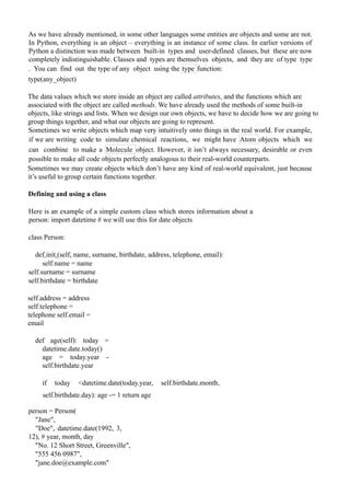


![# Python code to test that
# tuples are immutable
tuple
1 =(0, 1, 2,
3)
tuple1[0]
=4
print(tuple
1) Error :
Traceback (most recent call last):
File "e0eaddff843a8695575daec34506f126.py", line 3,
in tuple1[0]=4
TypeError: 'tuple' object does not support item
assignment filter_none
ed
it
pl
ay
_a
rr
o
w
br
ig
ht
ne
ss
_4
# Python code to test that
# strings are immutable
message ="Welcome to
GeeksforGeeks" message[0] ='p'
print(message) Error :
Traceback (most recent call last):
File "/home/ff856d3c5411909530c4d328eeca165b.py", line 3, in
message[0] = 'p'
TypeError: 'str' object does not support item assignment
Mutable Objects : These are of type list, dict, set . Custom classes are generally mutable.
# Python
code to test
that # lists are
mutable
color =["red", "blue",
"green"] print(color)
color[
0]
="pin](https://image.slidesharecdn.com/aintroductionbookofpythonforbeginners-250613145832-83400372/85/A-Introduction-Book-of-python-For-Beginners-docx-173-320.jpg)
![k"
color[
-1]
="ora
nge"
print(
color)
Output:['red', 'blue', 'green']
['pink', 'blue', 'orange']
Python Classes/Objects
Python is an object oriented programming language.
Almost everything in Python is an object, with its properties
and methods. A Class is like an object constructor, or a
"blueprint" for creating objects.
Create a Class
To create a class, use the keyword
class: Example
Create a class named MyClass, with a
property named x: class MyClass: x = 5
Create Object
Now we can use the class named MyClass to create
objects: Example
Create an object named p1, and print the value of x:
p1=MyClas
s()
print(p1.x)
The init () Function
The examples above are classes and objects in their simplest form, and are not really useful in real
life applications.
To understand the meaning of classes we have to understand the built-in init () function.
All classes have a function called init (), which is always executed when the class is being initiated.
Use the init () function to assign values to object properties, or other operations that are
necessary to do when the object is being created: Example
Create a class named Person, use the init () function to assign values for name
and age: class Person:
def init (self,name,age):
self.name=name
self.age=age
p1=Person("John", 36)
print(p1.name)
print(p1.age)
Object Methods
Objects can also contain methods. Methods in objects are functions that belong
to the object. Let us create a method in the Person class: Example
Insert a function that prints a greeting, and execute it on the p1 object:
class Person:
def init (self,name,age):](https://image.slidesharecdn.com/aintroductionbookofpythonforbeginners-250613145832-83400372/85/A-Introduction-Book-of-python-For-Beginners-docx-174-320.jpg)


![a
l
;
}
Consider the below example
filter_none
ed
it
pl
ay
_a
rr
o
w
br
ig
ht
ne
ss
_4
for(len = 0; len<strlen(str); +
+len) printf("%c",
toupper(str[len]));
If “strlen()” function is not marked as pure function then compiler will invoke the “strlen()” function
with each iteration of the loop, and if function is marked as pure function then compiler knows that
value of “strlen()” function will be same for each call, that’s why compiler optimizes the for loop
and generates code like following.
intlen = strlen(str);
for(i = 0; i<len; +
+i) printf("%c",
toupper((str[i]));
Let us write our own pure function to calculate string length.
attribute ((pure)) size_tmy_strlen(constchar*str)
{ constc
har*pt
r =
str;
while(
*ptr)
++ptr;
return(ptr – str);
}
Marking function as pure says that the hypothetical function “my_strlen()” is safe to call fewer times
than the program says.
c.Modifiers:
Python - public, private and protected](https://image.slidesharecdn.com/aintroductionbookofpythonforbeginners-250613145832-83400372/85/A-Introduction-Book-of-python-For-Beginners-docx-179-320.jpg)


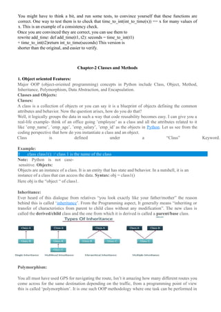

![ro
w
br
ig
ht
n
es
s
_
4
# Python program to demonstrate
# object printing
# Defining a class
classTest:
def init (self, a, b):
s
e
l
f
.
a
=
a
s
e
l
f
.
b
=
b
def repr (self):
return"Test a:% s b:% s"%(self.a, self.b)
def str (self):
return"From str method of Test: a is % s, "
"b is % s"%(self.a, self.b)
# Driver Code
t =Test(1234, 5678)
# This calls
str ()
print(t)
# This calls
repr ()
print([t])](https://image.slidesharecdn.com/aintroductionbookofpythonforbeginners-250613145832-83400372/85/A-Introduction-Book-of-python-For-Beginners-docx-185-320.jpg)

![print("Weight of {} is
{}".format(ram.name,ram.weight))
print(ram.eating("Pizza")) print("Weight of {}
is {}".format(steve.name,steve.height))
print("Weight of {} is
{}".format(steve.name,steve.weight))
print(steve.eating("Big Kahuna Burger"))
Output:
Height of Ramis6
Weight of Ramis60
Ramis eating Pizza
Weight of Steveis5.9
Weight of Steveis56
Steveis eating BigKahunaBurger
From str method of Test: a is 1234, b is 5678
[Test a:1234 b:5678]
Important Points about Printing:
Python uses repr method if there is no str
method. Example:
classTest:
def init (self, a, b):
self.a =a
self.b =b
def repr (self):
return"Test a:% s b:% s"%(self.a, self.b)
# Driver Code
t =Test(1234, 5678)
pr
int(t)
Output:
Test a:1234 b:5678
If no repr method is defined then the default is
used. Example:
classTest:
def init (self, a, b):
self.a =a
self.b =b
#
Driver Code
t
=Test(1234,
5678)
print(t)
Output:
< main .Test object at 0x7f9b5738c550>](https://image.slidesharecdn.com/aintroductionbookofpythonforbeginners-250613145832-83400372/85/A-Introduction-Book-of-python-For-Beginners-docx-187-320.jpg)


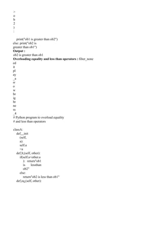


![def radd (self,
other): return self.
add (other) And
here’s how it’s
used:
>>> print 1337 + start10:07:17
7. Polymorphism in Python
What is Polymorphism?
The literal meaning of polymorphism is the condition of occurrence in different forms.
Polymorphism is a very important concept in programming. It refers to the use of a single type
entity (method, operator or object) to represent different types in different scenarios. Let's take an
example:
Example 1: Polymorphism in addition operator
We know that the + operator is used extensively in Python programs. But, it does not have a
single usage. For integer data types, + operator is used to perform arithmetic addition operation.
num1 =
1
num2 =
2
print(num1+num2
)
Run Code
Hence, the above program outputs 3.
Similarly, for string data types, + operator is used to perform
concatenation. str1 = "Python" str2 = "Programming"
print(str1+" "+str2)
Run Code
As a result, the above program outputs Python Programming .
Here, we can see that a single operator + has been used to carry out different operations for distinct
data types.
This is one of the most simple occurrences of polymorphism in Python.
Function Polymorphism in Python
There are some functions in Python which are compatible to run with multiple data types.
One such function is the function. It can run with many data types in Python. Let's look at
some example use cases of the function.
Example 2: Polymorphic len() function
print(len("Programiz")
)
print(len(["Python", "Java", "C"]))
print(len({"Name": "John", "Address":
"Nepal"}))
Run Code
Output
9
3
2
len(
)](https://image.slidesharecdn.com/aintroductionbookofpythonforbeginners-250613145832-83400372/85/A-Introduction-Book-of-python-For-Beginners-docx-199-320.jpg)


![# get
attrib
ute x
=MyI
nterfa
ce['x']
print(
x)
print(t
ype(x
))
Outp
ut :
<class
zope.interface.interface.Interface
Class> main MyInterface
<zope.interface.interface.Attribute object at 0x00000270A8C74358>
<class 'zope.interface.interface.Attribute'>
Implementing interface
Interface acts as a blueprint for designing classes, so interfaces are implemented using implementer
decorator on class. If a class implements an interface, then the instances of the class provide the interface.
Objects can provide interfaces directly, in addition to what their classes implement.
Syntax :
@zope.interface.implemente
r(*interfaces) class
Class_name: # methods
Example
filter_none
brightness
_4
importzop
e.interface
classMyInterface(zope.interfa
ce.Interface): x
=zope.interface.Attribute("
foo") defmethod1(self, x):
pass
defmethod2(self):
pass
@zope.interface.implementer(MyInterface)
classMyClass:
defmethod1(self,
x): returnx**2
defmethod2(self):
return"foo"
We declared that MyClass implements MyInterface. This means that instances of MyClass provide
MyInterface.
Methods
implementedBy(class) – returns a boolean value, True if class implements the interface else False
providedBy(object) – returns a boolean value, True if object provides the interface else False](https://image.slidesharecdn.com/aintroductionbookofpythonforbeginners-250613145832-83400372/85/A-Introduction-Book-of-python-For-Beginners-docx-205-320.jpg)
![True
False
True
[<InterfaceClass main .MyInterface>]
[<InterfaceClass main .MyInterface>]
[]
Interface Inheritance
Interfaces can extend other interfaces by listing the other interfaces as base interfaces. Functions
extends(interface) – returns boolean value, whether one interface extends another.
isOrExtends(interface) – returns boolean value, whether interfaces are same or one extends
another. isEqualOrExtendedBy(interface) – returns boolean value, whether interfaces are same
or one is extended by another. filter_none brightness_4
Import zope.interface
classBaseI(zope.interface.Interface):
defm1
(sel
f,
x):
pas
s
defm2(self):
pass
classDerivedI(BaseI
): defm3(self, x,
y):
pass
@zope.interface.implementer(Deri
vedI) classcls:
defm1(self, z):
returnz**3
defm2(self):
return'foo'
defm3(self, x, y):
returnx ^ y
# Get base interfaces
print(DerivedI. bases )
# Ask whether baseI extends
# DerivedI
print(BaseI.extends(DerivedI))
# Ask whether
baseI is equal to #
or is extended by
DerivedI
print(BaseI.isEqualOrExtendedBy(DerivedI))
# Ask whether baseI is equal to](https://image.slidesharecdn.com/aintroductionbookofpythonforbeginners-250613145832-83400372/85/A-Introduction-Book-of-python-For-Beginners-docx-207-320.jpg)


![Hearts-->2
Diamonds--
>1 Clubs--
>0
An obvious feature of this mapping is that the suits map to integers in order, so we can compare
suits by comparing integers. The mapping for ranks is fairly obvious; each of the numerical ranks
maps to the corresponding integer, and for face cards:
Jack-->11
Queen-->12
King-->13
The reason we are using mathematical notation for these mappings is that they are not part of the
Python program. They are part of the program design, but they never appear explicitly in the code.
The class definition for the Card type looks like this:
classCard:
def__init__(self,
suit=0, rank=0):
self.suit=suit
self.rank=rank
As usual, we provide an initialization method that takes an optional parameter for
each attribute. To create an object that represents the 3 of Clubs, use this command:
three_of_clubs=Card(0, 3)
The first argument, 0, represents the suit Clubs.
2.Class attributes and the __str__ method
In order to print Card objects in a way that people can easily read, we want to map the integer codes
onto words. A natural way to do that is with lists of strings. We assign these lists to class attributes
at the top of the class definition:
classCard:
SUITS= ('Clubs', 'Diamonds', 'Hearts', 'Spades')
RANKS= ('narf', 'Ace', '2', '3', '4', '5', '6', '7',
'8', '9', '10', 'Jack', 'Queen', 'King']
def__init__(self, suit=0, rank=0):
self.suit=suit
self.rank=rank
def__str__(self):
"""
>>>print(Card(2
, 11)) Queen
of Hearts
""" return'{0} of
{1}'.format(Card.RANKS[self.rank],
Card.SUITS[self.suit])
i
f__name__=='__m
ain__':
importdoctest
doctest.testmod()
Class attributes like Card.SUITS and Card.RANKS are defined outside of any method, and can be
accessed from any of the methods in the class.](https://image.slidesharecdn.com/aintroductionbookofpythonforbeginners-250613145832-83400372/85/A-Introduction-Book-of-python-For-Beginners-docx-210-320.jpg)
![Inside __str__, we can use SUITS and RANKS to map the numerical values of suit and rank to
strings. For example, the expression Card.SUITS[self.suit] means use the attribute suit from the
object self as an index into the class attribute named SUITS, and select the appropriate string.
The reason for the "narf" in the first element in ranks is to act as a place keeper for the zero-eth
element of the list, which will never be used. The only valid ranks are 1 to 13. This wasted item is
not entirely necessary. We could have started at 0, as usual, but it is less confusing to encode 2 as 2,
3 as 3, and so on.
We have a doctest in the __str__ method to confirm that Card(2, 11) will display as “Queen of
Hearts”.
3. Comparing cards
For primitive types, there are conditional operators ( <, >, ==, etc.) that compare values and determine
when one is greater than, less than, or equal to another. For user-defined types, we can override the
behavior of the built-in operators by providing a method named __cmp__. By convention,
__cmp__ takes two parameters, self and other, and returns 1 if the first object is greater, -1 if the
second object is greater, and 0 if they are equal to each other.
Some types are completely ordered, which means that you can compare any two elements and tell
which is bigger. For example, the integers and the floating-point numbers are completely ordered.
Some sets are unordered, which means that there is no meaningful way to say that one element is
bigger than another. For example, the fruits are unordered, which is why you cannot compare apples
and oranges.
The set of playing cards is partially ordered, which means that sometimes you can compare cards
and sometimes not. For example, you know that the 3 of Clubs is higher than the 2 of Clubs, and the
3 of Diamonds is higher than the 3 of Clubs. But which is better, the 3 of Clubs or the 2 of
Diamonds? One has a higher rank, but the other has a higher suit.
In order to make cards comparable, you have to decide which is more important, rank or suit. To be
honest, the choice is arbitrary. For the sake of choosing, we will say that suit is more important,
because a new deck of cards comes sorted with all the Clubs together, followed by all the
Diamonds, and so on. With that decided, we can write __cmp__: def__cmp__(self, other):
# check the suits
ifself.suit>other.suit:
return1
ifself.suit<other.suit:
return-1 # suits are
the same... check
ranks
i
fself.rank>other.rank
: return1
i
fself.rank<other.rank
: return-1 # ranks
are the same... it's a
tie return0
In this ordering, Aces appear lower than Deuces (2s).
4. Decks:
Now that we have objects to represent Cards, the next logical step is to define a class to represent a
Deck. Of course, a deck is made up of cards, so each Deck object will contain a list of cards as an
attribute.
The following is a class definition for the Deck class. The initialization method creates the
attribute cards and generates the standard set of fifty-two cards: classDeck: def__init__(self):](https://image.slidesharecdn.com/aintroductionbookofpythonforbeginners-250613145832-83400372/85/A-Introduction-Book-of-python-For-Beginners-docx-211-320.jpg)
![self.cards= []
forsuitinrange(4):
forrankinrange(1,
14):
self.cards.append(Car
d(suit, rank))
The easiest way to populate the deck is with a nested loop. The outer loop enumerates the suits from
0 to 3. The inner loop enumerates the ranks from 1 to 13. Since the outer loop iterates four times,
and the inner loop iterates thirteen times, the total number of times the body is executed is fifty-two
(thirteen times four). Each iteration creates a new instance of Card with the current suit and rank,
and appends that card to the cards list. The append method works on lists but not, of course, tuples.
5. Printing the deck
As usual, when we define a new type of object we want a method that prints the contents of an
object. To print a Deck, we traverse the list and print each Card: classDeck:
...
de
fprint_de
ck(self):
fo
rcardinse
lf.cards:
prin
t(card)
Here, and from now on, the ellipsis ( ...) indicates that we have omitted the other methods in the
class.
As an alternative to print_deck, we could write a __str__ method for the Deck class. The advantage
of __str__ is that it is more flexible. Rather than just printing the contents of the object, it generates
a string representation that other parts of the program can manipulate before printing, or store for
later use.
Here is a version of __str that returns a string representation of a Deck. To add a bit of pizzazz, it
arranges the cards in a cascade where each card is indented one space more than the previous card:
classDeck:
...
de
f__str
__(se
lf):
s=""
fo
riinrange(len(self.c
ards)):
s+=" "*i+str(self.cards[i])
+"n" returns
This example demonstrates several features. First, instead of traversing self.cards and assigning each
card to a variable, we are using i as a loop variable and an index into the list of cards.
Second, we are using the string multiplication operator to indent each card by one more space than
the last. The expression " " * i yields a number of spaces equal to the current value of i.
Third, instead of using the print function to print the cards, we use the str function. Passing an object
as an argument to str is equivalent to invoking the __str method on the object.
Finally, we are using the variable s as an accumulator. Initially, s is the empty string. Each time
through the loop, a new string is generated and concatenated with the old value of s to get the new](https://image.slidesharecdn.com/aintroductionbookofpythonforbeginners-250613145832-83400372/85/A-Introduction-Book-of-python-For-Beginners-docx-212-320.jpg)
![value. When the loop ends, s contains the complete string representation of the Deck, which looks
like this: >>>deck=Deck()
>>>print(deck)
Ace of Clubs
2 of Clubs
3 of Clubs
4 of Clubs
5 of Clubs
6 of Clubs
7 of Clubs
8 of Clubs
9 of Clubs
10 of Clubs
Jack of Clubs
Queen of Clubs
King of Clubs
Ace of Diamonds
And so on. Even though the result appears on 52 lines, it is one long string that contains newlines.
5.Shuffling the deck
If a deck is perfectly shuffled, then any card is equally likely to appear anywhere in the deck, and
any location in the deck is equally likely to contain any card.
To shuffle the deck, we will use the randrange function from the random module. With two
integer arguments, a and b, randrange chooses a random integer in the range a <= x < b. Since the
upper bound is strictly less than b, we can use the length of a list as the second parameter, and we
are guaranteed to get a legal index. For example, this expression chooses the index of a random card
in a deck: random.randrange(0, len(self.cards))
An easy way to shuffle the deck is by traversing the cards and swapping each card with a randomly
chosen one. It is possible that the card will be swapped with itself, but that is fine. In fact, if we
precluded that possibility, the order of the cards would be less than entirely random: classDeck:
...
de
fshuf
fle(se
lf):
impo
rtra
ndo
m
num_cards=len(self.cards)
foriinrange(num_cards):
j=random.randrange(i,
num_cards)
self.cards[i], self.cards[j] =self.cards[j], self.cards[i]
Rather than assume that there are fifty-two cards in the deck, we get the actual length of the list and
store it in num_cards.
For each card in the deck, we choose a random card from among the cards that haven’t been shuffled
yet. Then we swap the current card ( i) with the selected card ( j). To swap the cards we use a tuple
assignment:
self.cards[i], self.cards[j] =self.cards[j], self.cards[i].](https://image.slidesharecdn.com/aintroductionbookofpythonforbeginners-250613145832-83400372/85/A-Introduction-Book-of-python-For-Beginners-docx-213-320.jpg)


![Another use of conditional expressions is handling optional arguments. For example, here is the init
method from GoodKangaroo def init (self, name, contents=None): self.name = name if contents ==
None:
contents =
[]
self.pouch_contents
= contents We can
rewrite this one like
this:
def init (self, name, contents=None):
self.name = name
self.pouch_contents = [] if contents == None else contents
In general, you can replace a conditional statement with a conditional expression if both branches
contain simple expressions that are either returned or assigned to the same variable.
2. List comprehensions
In we saw the map and filter patterns. For example, this function takes a list of strings, maps the
string method capitalize to the elements, and returns a new list of strings:
def
capi
taliz
e_al
l(t):
res
= []
for
s in
t:
res.append(s.capit
alize()) return
res
We can write this more concisely using a list comprehension:
def capitalize_all(t):
return [s.capitalize() for s in t]
The bracket operators indicate that we are constructing a new list. The expression inside the
brackets specifies the elements of the list, and the for clause indicates what sequence we are
traversing.
The syntax of a list comprehension is a little awkward because the loop variable, s in this example,
appears in the expression before we get to the definition.
List comprehensions can also be used for filtering. For example, this function selects only the
elements of t that are upper case, and returns a new list:
def only_upper(t):
r
e
s
=
[
]
f
o](https://image.slidesharecdn.com/aintroductionbookofpythonforbeginners-250613145832-83400372/85/A-Introduction-Book-of-python-For-Beginners-docx-231-320.jpg)
![r
s
i
n
t
:
if s.isupper():
res.ap
pen
d(s)
retu
rn
res
We can rewrite it using a list
comprehension def
only_upper(t): return [s for s in
t if s.isupper()]
List comprehensions are concise and easy to read, at least for simple expressions. And they are
usually faster than the equivalent for loops, sometimes much faster. So if you are mad at me for not
mentioning them earlier, I understand. But, in my defense, list comprehensions are harder to debug
because you can’t put a print statement inside the loop. I suggest that you use them only if the
computation is simple enough that you are likely to get it right the first time. And for beginners that
means never.
3. Generator expressions
Generator expressions are similar to list comprehensions, but with parentheses instead of square
brackets:
>>> g = (x**2 for x in range(5))
>>> g
<generator object <genexpr> at 0x7f4c45a786c0>
The result is a generator object that knows how to iterate through a sequence of values. But unlike a
list comprehension, it does not compute the values all at once; it waits to be asked. The built-in
function next gets the next value from the generator:
>>> next(g)
0
>>> next(g)
1
When you get to the end of the sequence, next raises a StopIteration exception. You can also use a
for loop to iterate through the values:
>>> for val in g:
... print(val)
4
9
16
The generator object keeps track of where it is in the sequence, so the for loop picks up where next
left off. Once the generator is exhausted, it continues to raise StopIteration:
>>> next(g)
StopIteration](https://image.slidesharecdn.com/aintroductionbookofpythonforbeginners-250613145832-83400372/85/A-Introduction-Book-of-python-For-Beginners-docx-232-320.jpg)
![Generator expressions are often used with functions like sum, max, and min:
>>>sum(x**2 for x in range(5))
30
4. any and all
Python provides a built-in function, any, that takes a sequence of boolean values and returns True if
any of the values are True. It works on lists:
>>>any([False, False, True])
True
But it is often used with generator expressions:
>>>any(letter == 't' for letter in 'monty')
True
That example isn’t very useful because it does the same thing as the in operator. But we could use
any to rewrite some of the search functions we wrote in Section 9.3. For example, we could write
avoids like this:
def avoids(word, forbidden): return not
any(letter in forbidden for letter in
word)
The function almost reads like English, “word avoids forbidden if there are not any forbidden letters
in word.”
Using any with a generator expression is efficient because it stops immediately if it finds a True
value, so it doesn’t have to evaluate the whole sequence.
Python provides another built-in function, all, that returns True if every element of the sequence is
True. As an exercise, use all to re-write uses_all
5. Sets
I use dictionaries to find the words that appear in a document but not in a word list. The function I
wrote takes d1, which contains the words from the document as keys, and d2, which contains the
list of words. It returns a dictionary that contains the keys from d1 that are not in d2.
def
subt
ract(
d1,
d2):
res
=
dict(
) for
key
in
d1:
if key not in d2:
res[key] = None
return res
In all of these dictionaries, the values are None because we never use them. As a result, we waste
some storage space.
Python provides another built-in type, called a set, that behaves like a collection of dictionary keys
with no values. Adding elements to a set is fast; so is checking membership. And sets provide
methods and operators to compute common set operations.
For example, set subtraction is available as a method called difference or as an operator, -. So
we can rewrite subtract like this: def subtract(d1, d2):
return set(d1) - set(d2)
The result is a set instead of a dictionary, but for operations like iteration, the behavior is the same.
Some of the exercises in this book can be done concisely and efficiently with sets. For example,
here is a solution to has_duplicates, that uses a dictionary:](https://image.slidesharecdn.com/aintroductionbookofpythonforbeginners-250613145832-83400372/85/A-Introduction-Book-of-python-For-Beginners-docx-233-320.jpg)
![def
has_d
uplic
ates(t
): d =
{} for
x in t:
if x in d:
return True
d[x] = True
return False
When an element appears for the first time, it is added to the dictionary. If the same element appears
again, the function returns True.
Using sets, we can write the same function like this:
def has_duplicates(t):
return len(set(t)) <len(t)
An element can only appear in a set once, so if an element in t appears more than once, the set
will be smaller than t. If there are no duplicates, the set will be the same size as t. For example,
here’s a version of uses_only with a loop: def uses_only(word, available): for letter in word:
if letter not in available:
return False
return True
uses_only checks whether all letters in word are in available. We can rewrite it like this:
def uses_only(word, available):
return set(word) <= set(available)
The <= operator checks whether one set is a subset of another, including the possibility that they are
equal, which is true if all the letters in word appear in available. As an exercise, rewrite avoids using
sets.
6. Counters
A Counter is like a set, except that if an element appears more than once, the Counter keeps track of
how many times it appears. If you are familiar with the mathematical idea of a multiset, a Counter
is a natural way to represent a multiset.
Counter is defined in a standard module called collections, so you have to import it. You can
initialize a Counter with a string, list, or anything else that supports iteration:
>>> from collections import Counter
>>> count = Counter('parrot')
>>> count
Counter({'r': 2, 't': 1, 'o': 1, 'p': 1, 'a': 1})
Counters behave like dictionaries in many ways; they map from each key to the number of times it
appears. As in dictionaries, the keys have to be hashable.
Unlike dictionaries, Counters don’t raise an exception if you access an element that doesn’t appear.
Instead, they return 0: >>> count['d']
0
We can use Counters to rewrite
is_anagram : def
is_anagram(word1, word2):
return Counter(word1) ==
Counter(word2)](https://image.slidesharecdn.com/aintroductionbookofpythonforbeginners-250613145832-83400372/85/A-Introduction-Book-of-python-For-Beginners-docx-234-320.jpg)
![If two words are anagrams, they contain the same letters with the same counts, so their Counters are
equivalent. Counters provide methods and operators to perform set-like operations, including
addition, subtraction, union and intersection. And they provide an often-useful method,
most_common, which returns a list of value- frequency pairs, sorted from most common to least:
>>> count = Counter('parrot')
>>> for val, freq in count.most_common(3):
... print(val, freq)
r
2
p
1
a
1
7. defaultdict
The collections module also provides defaultdict, which is like a dictionary except that if you access
a key that doesn’t exist, it can generate a new value on the fly.
When you create a defaultdict, you provide a function that’s used to create new values. A function used to
create objects is sometimes called a factory. The built-in functions that create lists, sets, and other types
can be used as factories:
>>> from collections import defaultdict
>>> d = defaultdict(list)
Notice that the argument is list, which is a class object, not list(), which is a new list. The function
you provide doesn’t get called unless you access a key that doesn’t exist. >>> t = d['new key']
>>> t
[]
The new list, which we’re calling t, is also added to the dictionary. So if we modify t, the change
appears in d: >>>t.append('new value')
>>> d
defaultdict(<class 'list'>, {'new key': ['new value']})
If you are making a dictionary of lists, you can often write simpler code using defaultdict. In my
solution to, which you can get from http://thinkpython2.com/code/anagram_sets.py, I make a
dictionary that maps from a sorted string of letters to the list of words that can be spelled with those
letters. For example, ’opst’ maps to the list [’opts’, ’post’, ’pots’, ’spot’, ’stop’, ’tops’]. Here’s the
original code:
def
all_anagrams(f
ilename): d =
{} for line in
open(filename)
: word =
line.strip().low
er() t =
signature(word
) if t not in d:
d[t] = [word]
else:
d[t].append(word)](https://image.slidesharecdn.com/aintroductionbookofpythonforbeginners-250613145832-83400372/85/A-Introduction-Book-of-python-For-Beginners-docx-235-320.jpg)
![return d
This can be simplified using setdefault, which you might have used in Exercise 2:
def
all_anagrams(f
ilename): d =
{} for line in
open(filename)
: word =
line.strip().low
er() t =
signature(word
)
d.setdefault(t,
[]).append(word)
return d
This solution has the drawback that it makes a new list every time, regardless of whether it is
needed. For lists, that’s no big deal, but if the factory function is complicated, it might be. We
can avoid this problem and simplify the code using a defaultdict:
def
all_anagrams(f
ilename): d =
defaultdict(list)
for line in
open(filename)
: word =
line.strip().low
er() t =
signature(word
)
d[t].append(wo
rd)
return d
My solution to, which you can download from
http://thinkpython2.com/code/PokerHandSoln.py, uses setdefault in the function has_straightflush.
This solution has the drawback of creating a Hand object every time through the loop, whether it is
needed or not. As an exercise, rewrite it using a defaultdict. 8. Named tuples
Many simple objects are basically collections of related values. For example, the Point object
defined in contains two numbers, x and y. When you define a class like this, you usually start with
an init method and a str method:
class Point:
def init
(self, x=0,
y=0): self.x
= x self.y =
y
def str (self):
return '(%g, %g)' % (self.x, self.y)
This is a lot of code to convey a small amount of information. Python provides a more concise way
to say the same thing:
from collections import namedtuple
Point = namedtuple('Point', ['x', 'y'])](https://image.slidesharecdn.com/aintroductionbookofpythonforbeginners-250613145832-83400372/85/A-Introduction-Book-of-python-For-Beginners-docx-236-320.jpg)
![The first argument is the name of the class you want to create. The second is a list of the attributes
Point objects should have, as strings. The return value from namedtuple is a class object:
>>> Point
<class ' main .Point'>
Point automatically provides methods like init and str so you don’t have to write
them. To create a Point object, you use the Point class as a function:
>>> p = Point(1, 2)
>>> p
Point(x=1, y=2)
The init method assigns the arguments to attributes using the names you provided. The str
method prints a representation of the Point object and its attributes. You can access the
elements of the named tuple by name:
>>>p.x, p.y
(1, 2)
But you can also treat a named tuple as a tuple:
>>>p[0], p[1]
(1, 2)
>>> x, y = p
>>> x, y
(1, 2) Named tuples provide a quick way to define simple classes. The drawback is that simple
classes don’t always stay simple. You might decide later that you want to add methods to a named
tuple. In that case, you could define a new class that inherits from the named tuple:
class Pointier(Point):
# add more methods here
Or you could switch to a conventional class definition.
9.Gathering keyword args we saw how to write a
function that gathers its arguments into a tuple:
def printall(*args): print(args) You can call this function with any number of positional
arguments (that is, arguments that don’t have keywords):
>>>printall(
1, 2.0, '3')
(1, 2.0, '3')
But the * operator doesn’t gather keyword arguments:
>>>printall(1, 2.0, third='3')
TypeError: printall() got an unexpected keyword
argument 'third' To gather keyword arguments, you
can use the ** operator: def printall(*args,
**kwargs): print(args, kwargs)
You can call the keyword gathering parameter anything you want, but kwargs is a common choice.
The result is a dictionary that maps keywords to values:
>>>printall(1, 2.0, third='3')
(1, 2.0) {'third': '3'}
If you have a dictionary of keywords and values, you can use the scatter operator, ** to call a
function:
>>> d = dict(x=1, y=2)
>>> Point(**d)
Point(x=1, y=2)
Without the scatter operator, the function would treat d as a single positional argument, so it
would assign d to x and complain because there’s nothing to assign to y:
>>> d = dict(x=1, y=2)
>>> Point(d)](https://image.slidesharecdn.com/aintroductionbookofpythonforbeginners-250613145832-83400372/85/A-Introduction-Book-of-python-For-Beginners-docx-237-320.jpg)

A Introduction Book of python For Beginners.docx
- 1. PYTHON PROGRAMMING Python Introduction Release Basic of Python : a Introduction of Basic Python May 2024
- 2. Unit – I Introduction: What is a program, Running python, Arithmetic operators, Value and Types. Variables, Assignments and Statements: Assignment statements, Script mode, Order of operations, string operations, comments. Functions: Function calls, Math functions, Composition, Adding new Functions, Definitions and Uses, Flow of Execution, Parameters and Arguments, Variables and Parameters are local, Stack diagrams, Fruitful Functions and Void Functions, Why Functions. Unit – II Case study: The turtle module, Simple Repetition, Encapsulation, Generalization, Interface design, Refactoring, docstring. Conditionals and Recursion: floor division and modulus, Boolean expressions, Logical operators, Conditional execution, Alternative execution, Chained conditionals, Nested conditionals, Recursion, Infinite Recursion, Keyboard input. Fruitful Functions: Return values, Incremental development, Composition, Boolean functions, More recursion, Leap of Faith, Checking types. Unit – III Iteration: Reassignment, Updating variables, The while statement, Break, Square roots, Algorithms. Strings: A string is a sequence, len, Traversal with a for loop, String slices, Strings are immutable, Searching, Looping and Counting, String methods, The in operator, String comparison. Case Study: Reading word lists, Search, Looping with indices. Lists: List is a sequence, Lists are mutable, Traversing a list, List operations, List slices, List methods, Map filter and reduce, Deleting elements, Lists and Strings, Objects and values, Aliasing, List arguments. Unit – IV Dictionaries: A dictionary is a mapping, Dictionary as a collection of counters, Looping and dictionaries, Reverse Lookup, Dictionaries and lists, Memos, Global Variables. Tuples: Tuples are immutable, Tuple Assignment, Tuple as Return values, Variable-length argument tuples, Lists and tuples, Dictionaries and tuples, Sequences of sequences. Files: Persistence, Reading and writing, Format operator, Filename and paths, Catching exceptions, Databases, Pickling, Pipes, Writing modules. Classes and Objects: Programmer-defined types, Attributes, Instances as Return values, Objects are mutable, Copying. Unit – V Classes and Functions: Time, Pure functions, Modifiers, Prototyping versus Planning Classes and Methods: Object oriented features, Printing objects, The init method, The str method, Operator overloading, Type-based Dispatch, Polymorphism, Interface and Implementation Inheritance: Card objects, Class attributes, Comparing cards, decks, Printing the Deck, Add Remove shuffle and sort, Inheritance, Class diagrams, Data encapsulation. The Goodies: Conditional expressions, List comprehensions, Generator expressions, any and all, Sets, Counters, defaultdict, Named tuples, Gathering keyword Args, Unit 1 Chapter-1 INTRODUCTION What Is a Program A program is a sequence of instructions that specifies how to perform a computation.
- 3. The computation might be something mathematical, such as solving a system of equations or finding the roots of a polynomial, but it can also be a symbolic computation, such as searching and replacing text in a document or something graphical, like processing an image or playing a video. few basic instructions appear in just about every language: input: Get data from the keyboard, a file, the network, or some other device. output: Display data on the screen, save it in a file, send it over the network, etc. math: Perform basic mathematical operations like addition and multiplication. conditional execution: Check for certain conditions and run the appropriate code. repetition: Perform some action repeatedly, usually with some variation. Install and Run Python: Installing Python Download the latest version of Python. Run the installer file and follow the steps to install Python During the install process, check Add Python to environment variables. This will add Python to environment variables, and you can run Python from any part of the computer. Also, you can choose the path where Python is installed. Installing Python on the computer Once you finish the installation process, you can run Python. 1. Run Python in Immediate mode Once Python is installed, typing python in the command line will invoke the interpreter in immediate mode. We can directly type in Python code, and press Enter to get the output. Try typing in 1 + 1 and press enter. We get 2 as the output. This prompt can be used as a calculator. To exit this mode, type quit() and press enter.
- 4. Running Python on the Command Line 2. Run Python in the Integrated Development Environment (IDE) IDE is a piece of software that provides useful features like code hinting, syntax highlighting and checking, file explorers, etc. to the programmer for application development. By the way, when you install Python, an IDE named IDLE is also installed. You can use it to run Python on your computer. It's a decent IDE for beginners. When you open IDLE, an interactive Python Shell is opened. Python IDLE Now you can create a new file and save it with .py extension. For example, hello.py Write Python code in the file and save it. To run the file, go to Run > Run Module or simply click F5. Running a Python program in IDLE The First Program: >>> print('Hello, World!') This is an example of a print statement the result is the words Hello, World! The quotation marks in the program mark the beginning and end of the text to be displayed; they don’t appear in the result. The parentheses indicate that print is a function. Operators: Python language supports the following types of operators. Arithmetic Operators Comparison (Relational) Operators Assignment Operators Logical Operators Bitwise Operators Membership Operators Identity Operators Let us have a look on all operators one by one.
- 5. Python Arithmetic Operators Assume variable a holds 10 and variable b holds 20, then – Operator Description Example + Addition Adds values on either side of the operator. a + b = 30 - Subtraction Subtracts right hand operand from left hand operand. a – b = -10 * Multiplicatio n Multiplies values on either side of the operator a * b = 200 / Division Divides left hand operand by right hand operand b / a = 2 % Modulus Divides left hand operand by right hand operand and returns remainder b % a = 0 ** Exponent Performs exponential (power) calculation on operators a**b =10 to the power 20 // Floor Division - The division of operands where the result is the quotient in which the digits after the decimal point are removed. But if one of the operands is negative, the result is floored, i.e., rounded away from zero (towards negative infinity) − 9//2 = 4 and 9.0//2.0 = 4.0, -11//3 = -4, -11.0//3 = -4.0 Values and Types A value is one of the basic things a program works with, like a letter or a number. Some values we have seen so far are 2, 42.0, and 'Hello, World!' These values belong to different types: 2 is an integer, 42.0 is a floating-point number and 'Hello, World!' is a string If you are not sure what type a value has, the interpreter can tell you: >>> type(2) <class 'int'> >>> type(42.0) <class 'float'> >>> type('Hello, World!') <class 'str'> In these results, the word “class” is used in the sense of a category; a type is a category of values. What about values like '2' and '42.0'? They look like numbers, but they are in quotation marks like strings: >>> type('2') <class 'str'> >>> type('42.
- 6. 0') <class 'str'> Therefore they’re strings. Chapter-2 Variables, Assignments and Statements 1.An assignment statement creates a new variable and gives it a value: >>> message = 'And now for something completely different' >>> n = 17 >>> pi = 3.141592653589793 This example makes three assignments. The first assigns a string to a new variable named message; the second gives the integer 17 to n; the third assigns the (approximate) value of π to pi Variable Names Programmers generally choose names for their variables that are meaningful Variable names can be as long as you like. Rules for naming : They can contain both letters and numbers,but they can’t begin with a number. Can use both lower and uppercase letters.The underscore character, _, can appear in a name. Keywords should not use as a variable name. Note: If you give a variable an illegal name, you get a syntax error: >>> 76trombones = 'big parade' SyntaxError: invalid syntax b’ coz it begins with a number >>> more@ = 1000000 SyntaxError: invalid syntax b’ coz it contains illegal character @. >>> class = 'Adanced Theoretical Zymurgy' Keywords in Python: False, class, finally, is, return, None, continue, for, lambda, try, True, def, from, nonlocal, while, and, del, global, not, with, as, elif, if, or, yield, assert, else, import, pass, break, except, in, raise. Expressions and Statements: An expression is a combination of values, variables, and operators. A value all by itself is considered an expression, and so is a variable, so the following are all legal expressions: >> 42 42 >>> n 17 > > > n + 2 5 4
- 7. 2 When you type an expression at the prompt, the interpreter evaluates it, which means that it finds the value of the expression. In this example, n has the value 17 and n + 25 has the value 42. A statement is a unit of code that has an effect, like creating a variable or displaying a value. >>> n = 17 >>> print(n) The first line is an assignment statement that gives a value to n. The second line is a print statement that displays the value of n. 2. Script Mode: Inscript mode type code in a file called a script and savefile with .py extention. script mode to execute the script. By convention, Python scripts have names that end with .py. for ex: if you type the following code into a script and run it, you get no output at all. Why because but it doesn’t display the value unless you tell it to. But it displays in interactive mode. miles = 26.2 miles * 1.61 Sol is: miles = 26.2 print(mile s * 1.61) 3. Order of perations: When an expression contains more than one operator, the order of evaluation depends on the order of operations.For mathematical operators, Python follows order PEMDAS. P-parentheses, E- Exponentiation, M- Multiplication D-Division A-Addition, S- Substraction • Parentheses have the highest precedence. For ex in the following expressions in parentheses are evaluated first, Ex:1. 2 * (3-1) is 4, and Ex: 2. (1+1)**(5-2) is 8. • Exponentiation has the next highest precedence, For ex: 1 + 2**3 is 9, not 27, and 2 * 3**2 is 18, not 36. • Multiplication and Division have higher precedence than Addition and Subtraction. For ex: 2*3-1 is 5, not 4, and 6+4/2 is 8, not 5. Note: Operators with the same precedence are evaluated from left to right (except exponentiation). So in the expression degrees / 2 * pi, the division happens first and the result is multiplied by pi. 4. Operations on strings:
- 8. Note : Mathematical operations on strings are not allowed so the following are illegal: '2'-'1' 'eggs'/'easy' 'third'*'a charm' How to Create Strings in Python? Creating strings is easy as you only need to enclose the characters either in single or double-quotes. In the following example, we are providing different ways to initialize strings.To share an important note that you can also use triple quotes to create strings. However, programmers use them to mark multi-line strings and docstrings. # Python string examples - all assignments are identical. String_var = 'Python' String_var = "Python" String_var = """Python""" # with Triple quotes Strings can extend to multiple lines String_var = """ This document will help you to explore all the concepts of Python Strings!!! """ # Replace "document" with "tutorial" and store in another variable substr_var = String_var.replace("document", "tutorial") print (substr_var) String Operators in Python Concatenation (+):It combines two strings into one. # ex a m pl e va r1 = 'P yt ho n' va r2 = 'St rin g' print (var1+var2) # PythonString Repetition (*):This operator creates a new string by repeating it a given number of times. # e x
- 9. a m p l e v a r 1 = ' P y t h o n' p ri n t ( v a r 1 * 3 ) # PythonPythonPython Slicing [ ]:The slice operator prints the character at a given index. # examp le var1 = 'Pytho n' print (var1[2]) # t Range Slicing [x:y] It prints the characters present in the given range. # example var1 = 'Python' print (var1[2: 5]) # tho Membership (in):This operator returns ‘True’ value if the character is present in the given String.
- 10. # example var1 = 'Python' print ('n' in var1) # True Membersh ip (not in): : It returns ‘True’ value if the character is not present in the given String. # exampl e var1 = 'Python ' print ('N' not in var1) # True Iterating (for): With this operator, we can iterate through all the characters of a string. # example for var in var1: print (var, end ="") # Python Raw String (r/R):We can use it to ignore the actual meaning of Escape characters inside a string. For this, we add ‘r’ or ‘R’ in front of the String. # example print (r'n') # n print (R'n') # n Unicode String support in Python egular Strings stores as the 8-bit ASCII value, whereas Unicode String follows the 16-bit ASCII standard. This extension allows the strings to include characters from the different languages of the world. In Python, the letter ‘u’ works as a prefix to distinguish between Unicode and usual strings. print (u' Hello Python!!')
- 11. OUTPUT: #Hello Python Python has a set of built-in methods that you can use on strings. Note: All string methods returns new values. They do not change the original string. center() Returns a centered string count() Returns the number of times a specified value occurs in a string encode() Returns an encoded version of the string endswith() Returns true if the string ends with the specified value expandtabs() Sets the tab size of the string find() Searches the string for a specified value and returns the position of where it was found format() Formats specified values in a string format_map() Formats specified values in a string index() Searches the string for a specified value and returns the position of where it was found isalnum() Returns True if all characters in the string are alphanumeric isalpha() Returns True if all characters in the string are in the alphabet
- 12. isdecimal() Returns True if all characters in the string are decimals isdigit() Returns True if all characters in the string are digits isidentifier() Returns True if the string is an identifier islower() Returns True if all characters in the string are lower case isnumeric() Returns True if all characters in the string are numeric isprintable() Returns True if all characters in the string are printable isspace() Returns True if all characters in the string are whitespaces istitle() Returns True if the string follows the rules of a title isupper() Returns True if all characters in the string are upper case join() Joins the elements of an iterable to the end of the string ljust() Returns a left justified version of the string
- 13. lower() Converts a string into lower case lstrip() Returns a left trim version of the string maketrans() Returns a translation table to be used in translations partition() Returns a tuple where the string is parted into three parts replace() Returns a string where a specified value is replaced with a specified value rfind() Searches the string for a specified value and returns the last position of where it was found rindex() Searches the string for a specified value and returns the last position of where it was found rjust() Returns a right justified version of the string rpartition() Returns a tuple where the string is parted into three parts rsplit() Splits the string at the specified separator, and returns a list rstrip() Returns a right trim version of the string
- 14. But there are two exceptions, + and *. The + operator performs string concatenation, For example: >>> first = 'throat' split() Splits the string at the specified separator, and returns a list splitlines() Splits the string at line breaks and returns a list startswith() Returns true if the string starts with the specified value strip() Returns a trimmed version of the string swapcase() Swaps cases, lower case becomes upper case and vice versa title() Converts the first character of each word to upper case translate() Returns a translated string upper() Converts a string into upper case zfill() Fills the string with a specified number of 0 values at the beginning >>> second = 'warbler' >>> first + second throatwar bler The * operator also works on strings; it performs repetition. For example, 'Spam'*3 is 'SpamSpamSpam'.
- 15. EXAMPLE1: var1 = 'Hello World!' var2 = "Python Programming" print "var1[0]: ", var1[0] print "var2[1:5]: ", var2[1:5] When the above code is executed, it produces the following result − var1[0]: H var2[1:5]: ytho EXAMPLE2: var1 = 'Hello World!' print "Updated String :- ", var1[:6] + 'Python' When the above code is executed, it produces the following result − Updated String :- Hello Python 5. Comments: Comments are of two types . Single-line comments Multi line Comments Single-line comments are created simply by beginning a line with the hash (#) character, and they are automatically terminated by the end of line. For Ex: #This would be a comment in Python Multi Line Comments that span multiple lines and are created by adding a delimiter (“””) on each end of the comment For Ex: """ This would be a multiline comment in Python that spans several lines and describes your code, your day, or anything you want it to """ Chapter-3 Functions What is a Function in Python? A Function in Python is used to utilize the code in more than one place in a program. It is also called method or procedures. Python provides you many inbuilt functions like print(), but it also gives freedom to create your own functions. Functions: A function is a named sequence of statements that performs a computation. How to define and call a function in Python Function in Python is defined by the "def " statement followed by the function name and parentheses ( () ) Example:
- 16. Let us define a function by using the command " def func1():" and call the function. The output of the function will be "I am learning Python function" The function print func1() calls our def func1(): and print the command " I am learning Python function None."There are set of rules in Python to define a function.Any args or input parameters should be placed within these parentheses.The function first statement can be an optional statement- docstring or the documentation string of the function The code within every function starts with a colon (:) and should be indented (space) The statement return (expression) exits a function, optionally passing back a value to the caller. A return statement with no args is the same as return None. Significance of Indentation (Space) in Python: Before we get familiarize with Python functions, it is important that we understand the indentation rule to declare Python functions and these rules are applicable to other elements of Python as well like declaring conditions, loops or variable. Python follows a particular style of indentation to define the code, since Python functions don't have any explicit begin or end like curly braces to indicate the start and stop for the function, they have to rely on this indentation. Here we take a simple example with "print" command. When we write "print" function right below the def func 1 (): It will show an "indentation error: expected an indented block". Now, when you add the indent (space) in front of "print" function, it should print as expected. How Function Return Value? Return command in Python specifies what value to give back to the caller of the function. Let's understand this with the following example Step 1) Here - we see when function is not "return". For example, we want the square of 4, and it should give answer "16" when the code is executed. Which it gives when we simply use "print x*x" code, but when you call function "print square" it gives "None" as an output. This is because when you call the function, recursion does not happen and fall off the end of the function. Python returns "None" for failing off the end of the function. Step 2) To make this clearer we replace the print command with assignment command. Let's check the output. When you run the command "print square (4)" it actually returns the value of the object since we don't have any specific function to run over here it returns "None". Step 3) Now, here we will see how to retrieve the output using "return" command. When you use the "return" function and execute the code, it will give the output "16." Step 4) Functions in Python are themselves an object, and an object has some value. We will here see how Python treats an object. When you run the command "print square" it returns the value of the object. Since we have not passed any argument, we don't have any specific function to run over here it returns a default value (0x021B2D30) which is the location of the object. In practical Python program, you probably won't ever need to do this.
- 17. Arguments in Functions The argument is a value that is passed to the function when it's called.In other words on the calling side, it is an argument and on the function side it is a parameter. Let see how Python Args works - Step 1) Arguments are declared in the function definition. While calling the function, you can pass the values for that args as shown below Step 2) To declare a default value of an argument, assign it a value at function definition. Example: x has no default values. Default values of y=0. When we supply only one argument while calling multiply function, Python assigns the supplied value to x while keeping the value of y=0. Hence the multiply of x*y=0 Step 3) This time we will change the value to y=2 instead of the default value y=0, and it will return the output as (4x2)=8. Step 4) You can also change the order in which the arguments can be passed in Python. Here we have reversed the order of the value x and y to x=4 and y=2. Step 5) Multiple Arguments can also be passed as an array. Here in the example we call the multiple args (1,2,3,4,5) by calling the (*args) function. Example: We declared multiple args as number (1,2,3,4,5) when we call the (*args) function; it prints out the output as (1,2,3,4,5) Rules to define a function in Python. Function blocks begin with the keyword def followed by the function name and parentheses ( ( ) ).Any input parameters or arguments should be placed within these parentheses. You can also define parameters inside these parentheses.The code block within every function starts with a colon (:) and is indented. The statement return [expression] exits a function, but it is optional Syntax: def functionname( parameters ): functio n_suite return [expres sion] Creati ng a Functi on In Python a function is defined using the def keyword: Example def my_function(): print("Hello from a function") Calling a Function To call a function, use the function name followed by parenthesis: Example def my_function(): print("Hello from a function") my_function() #calling function
- 18. Scope and Lifetime of variables Scope of a variable is the portion of a program where the variable is recognized. Parameters and variables defined inside a function are not visible from outside the function. Hence, they have a local scope. The lifetime of a variable is the period throughout which the variable exits in the memory. The lifetime of variables inside a function is as long as the function executes.They are destroyed once we return from the function. Hence, a function does not remember the value of a variable from its previous calls.Here is an example to illustrate the scope of a variable inside a function. def my_func(): x = 10 print("Value inside function:",x) x = 20 my _fu nc() print("Value outside function:",x) Output Value inside function: 10 Value outside function: 20 2. Math Functions: Python has a math module that provides mathematical functions. A module is a file that contains a collection of related functions.Before we can use the functions in a module, we have to import it with an import statement: >>> import math Note: The module object contains the functions and variables defined in the module. To access one of the functions, you have to specify the name of the module and the name of the function, separated by a dot (also known as a period). This format is called dot notation. For ex: >>> ratio = signal_power / noise_power >>> decibels = 10 * math.log10(ratio) >>> radians = 0.7 >>> height = math.sin(radians) Some Constants These constants are used to put them into our calculations. Sr.No. Constants & Description 1 pi - Return the value of pi: 3.141592
- 19. 4 inf - Returns the infinite 5 nan - Not a number type. Numbers and Numeric Representation These functions are used to represent numbers in different forms. The methods are like below − Sr.No. Function & Description 1 ceil(x) Return the Ceiling value. It is the smallest integer, greater or equal to the number x. 3 fabs(x) Returns the absolute value of x. 4 factorial(x) Returns factorial of x. where x ≥ 0 5 floor(x) Return the Floor value. It is the largest integer, less or equal to the number x. 6 fsum(iterable) Find sum of the elements in an iterable object 7 gcd(x, y) Returns the Greatest Common Divisor of x and y 8 isfinite(x) Checks whether x is neither an infinity nor nan. 9 isinf(x) Checks whether x is infinity 10 isnan(x) Checks whether x is not a number. 11 remainder(x, y) Find remainder after dividing x by y Example program: import math print(math.ceil(23.56) ) my_list = [12, 4.25, 89, 3.02, -65.23, -7.2, 6.3] print(math.fsum(my_list)) print('The GCD of 24 and 56 : ' + str(math.gcd(24, 56))) x = float('nan') if math.isnan(x): print('It is not a number')
- 20. x = float('i nf') y = 45 if math.i sinf(x) : print(' It is Infinit y') print(math.isfinite(x)) #x is not a finite number print(math.isfinite(y)) #y is a finite number O/P: 24 42.13999999999999 The GCD of 24 and 56 : 8 It is not a number It is Infinity False True >>> Power and Logarithmic Functions These functions are used to calculate different power related and logarithmic related tasks. Sr.No. Function & Description 1 pow(x, y) Return the x to the power y value. 2 sqrt(x) Finds the square root of x 3 exp(x) Finds xe, where e = 2.718281 4 log(x[, base]) Returns the Log of x, where base is given. The default base is e 5 log2(x) Returns the Log of x, where base is 2 6 log10(x) Returns the Log of x, where base is 10 Example Code import math
- 21. print('The value of 5^8: ' + str(math.pow(5, 8))) print('Square root of 400: ' + str(math.sqrt(400))) print('The value of 5^e: ' + str(math.exp(5))) print('The value of Log(625), base 5: ' + str(math.log(625, 5))) print('The value of Log(1024), base 2: ' + str(math.log2(1024))) print('The value of Log(1024), base 10: ' + str(math.log10(1024))) Output The value of 5^8: 390625.0 Square root of 400: 20.0 The value of 5^e: 148.4131591025766 The value of Log(625), base 5: 4.0 The value of Log(1024), base 2: 10.0 The value of Log(1024), base 10: 3.010299956639812 Trigonometric & Angular Conversion Functions These functions are used to calculate different trigonometric operations. Sr.No. Function & Description 1 sin(x) Return the sine of x in radians 2 cos(x) Return the cosine of x in radians 3 tan(x) Return the tangent of x in radians 4 asin(x) This is the inverse operation of the sine, there are acos, atan also. 5 degrees(x) Convert angle x from radian to degrees 6 radians(x) Convert angle x from degrees to radian Example Code import math print('The value of Sin(60 degree): ' + str(math.sin(math.radians(60)))) print('The value of cos(pi): ' + str(math.cos(math.pi))) print('The value of tan(90 degree): ' + str(math.tan(math.pi/2))) print('The angle of sin(0.8660254037844386): ' + str(math.degrees(math.asin(0.8660254037844386)))) Output The value of Sin(60 degree): 0.8660254037844386
- 22. The value of cos(pi): -1.0 The value of tan(90 degree): 1.633123935319537e+16 The angle of sin(0.8660254037844386): 59.99999999999999 3. Composition: So far, we have looked at the elements of a program—variables, expressions, and statements—in isolation, without talking about how to combine(Composition) them.For example, the argument of a function can be any kind of expression, including arithmetic operators: x = math.sin(degrees / 360.0 * 2 * math.pi) And even function calls: x = math.exp(math.log(x+1)) 4. Adding new functions: Pass by reference vs value:All parameters (arguments) in the Python language are passed by reference. It means if you change what a parameter refers to within a function, the change also reflects back in the calling function. For example − #!/usr/bin/python # Function definition is here def changeme( mylist ): "This changes a passed list into this function" mylist.append([1,2,3,4]); print "Values inside the function: ", mylist return # Now you can call changeme function mylist = [10,20,30]; changeme( mylist ); print "Values outside the function: ", mylist Here, we are maintaining reference of the passed object and appending values in the same object. So, this would produce the following result − Values inside the function: [10, 20, 30, [1, 2, 3, 4]] Values outside the function: [10, 20, 30, [1, 2, 3, 4]] Scope of Variables:All variables in a program may not be accessible at all locations in that program. This depends on where you have declared a variable.The scope of a variable determines the portion of the program where you can access a particular identifier. There are two basic scopes of variables in Python − Global variables Local variables Global vs. Local variables:Variables that are defined inside a function body have a local scope, and those defined outside have a global scope.This means that local variables can be accessed only inside the function in which they are declared,
- 23. whereas global variables can be accessed throughout the program body by all functions. When you call a function, the variables declared inside it are brought into scope. Following is a simple example − #!/usr/bin/python total = 0; # This is global variable. # Function definition is here def sum( arg1, arg2 ): # Add both the parameters and return them." total = arg1 + arg2; # Here total is local variable. print "Inside the function local total : ", total return total; # Now you can call sum function sum( 10, 20 ); print "Outside the function global total : ", total When the above code is executed, it produces the following result − Inside the function local total : 30 Outside the function global total : 0 The import Statement You can use any Python source file as a module by executing an import statement in some other Python source file. The import has the following syntax − import module1[, module2[,... moduleN] When the interpreter encounters an import statement, it imports the module if the module is present in the search path. A search path is a list of directories that the interpreter searches before importing a module. For example, to import the module support.py, you need to put the following command at the top of the script − #!/usr/bin/python # Import module support import support # Now you can call defined function that module as follows support.print_func("Zara") When the above code is executed, it produces the following result − Hello : Zara 5. Flow of Execution The order in which statements are executed is called the flow of execution Execution always begins at the first statement of the program. Statements are executed one at a time, in order, from top to bottom. Function definitions do not alter the flow of execution of the program, but remember that statements inside the function are not executed until the function is called.
- 24. Function calls are like a bypass in the flow of execution. Instead of going to the next statement, the flow jumps to the first line of the called function, executes all the statements there, and then comes back to pick up where it left off. 6. Parameters and Arguments: Parameter: The terms parameter and argument can be used for the same thing: information that are passed into a function.From a function's perspective: A parameter is the variable listed inside the parentheses in the function definition. An argument is the value that is sent to the function when it is called. Arguments You can call a function by using the following types of formal arguments – 1.Required arguments 2.Keyword arguments 3.Default arguments 4.Variable- length arguments Required arguments Required arguments are the arguments passed to a function in correct positional order. Here, the number of arguments in the function call should match exactly with the function definition. To call the function printme(), you definitely need to pass one argument, otherwise it gives a syntax error as follows − #!/usr/bin/python # Function definition is here def printme( str ): "This prints a passed string into this function" print str retur n; # Now you can call printme function printme() When the above code is executed, it produces the following result − Traceback (most recent call last): File "test.py", line 11, in <module> printme(); TypeError: printme() takes exactly 1 argument (0 given) Keyword arguments Keyword arguments are related to the function calls. When you use keyword arguments in a function call, the caller identifies the arguments by the parameter name. This allows you to skip arguments or place them out of order because the Python interpreter is able to use the keywords provided to match the values with parameters. You can also make keyword calls to the printme() function in the following ways − #!/usr/bin/python
- 25. # Function definition is here def printme( str ): "This prints a passed string into this function" print str return; # Now you can call printme function printme( str = "My string") When the above code is executed, it produces the following result − My string The following example gives more clear picture. Note that the order of parameters does not matter. #!/usr/bin/python # Function definition is here def printinfo( name, age ): "This prints a passed info into this function" print "Name: ", name print "Age ", age retur n; # Now you can call printinfo function printinfo( age=50, name="miki" ) When the above code is executed, it produces the following result − Name: miki Age 50 Default arguments A default argument is an argument that assumes a default value if a value is not provided in the function call for that argument. The following example gives an idea on default arguments, it prints default age if it is not passed − #!/usr/bin/python # Function definition is here def printinfo( name, age = 35 ): "This prints a passed info into this function" print "Name: ", name print "Age ", age retur n;
- 26. # Now you can call printinfo function printinfo( age=50, name="miki" ) printinfo( name="miki" ) When the above code is executed, it produces the following result − Name: miki Age 50 Name: miki Age 35 Variable-length arguments You may need to process a function for more arguments than you specified while defining the function. These arguments are called variable-length arguments and are not named in the function definition, unlike required and default arguments.Syntax for a function with non- keyword variable arguments is this − def functionname([formal_args,] *var_args_tuple ): "functi on_doc string" functio n_suite return [expres sion] An asterisk (*) is placed before the variable name that holds the values of all nonkeyword variable arguments. This tuple remains empty if no additional arguments are specified during the function call. Following is a simple example − #!/usr/bin/python # Function definition is here def printinfo( arg1, *vartuple ): "This prints a variable passed arguments" print "Out put is: " print arg1 for var in vartu ple: print var retur n; # Now you can call printinfo function
- 27. printinfo( 10 ) printinfo( 70, 60, 50 ) When the above code is executed, it produces the following result − Output is: 10 Output is: 70 60 50 Example def my_functio n(fname): print(fname + " krishna") my_function("Rama") my_function("Siva") my_function("Hari") o/p: Ramakrishna Sivakrishna Harikrishna. Parameters Vs Arguments A parameter is the variable listed inside the parentheses in the function definition. An argument is the value that is sent to the function when it is called. Number of Arguments A function must be called with the correct number of arguments. Meaning that if your function expects 2 arguments, you have to call the function with 2 arguments, not more, and not less. Example This function expects 2 arguments, and gets 2 arguments: def my_function(fname, lname): print(fname + " " + lname) my_function("Srinu", "vasulu") Arbitrary Arguments( *args) If you do not know how many arguments that will be passed into your function, add a * before the parameter name in the function definition. This way the function will receive a tuple of arguments, and can access the items accordingly: Example If the number of arguments is unknown, add a * before the parameter name: def my_function(*kids): print("The youngest child is " + kids[2]) my_function("raju", "somu", "vijay) O/p: vijay Default Parameter Value: When we call the function without argument, it uses the default value: Example def my_function(country = "Norway"): #default value is Norway print("I am from " + country) my_function("Sweden")
- 28. my_function("India") my_function() #o/p: Norway my_function("Brazil") Passing a List as an Argument: You can send any data types of argument to a function (string, number, list, dictionary etc.) E.g. if you send a List as an argument, it will still be a List when it reaches the function: Example def my_function(food): for x in food: prin t(x) fruits = my_function(fruits) Return Values: To return a value, we use the return statement: Example def my_function(x): ["apple", "banana", "cherry"] return 5 * x print(my_function(3)) # o/p: 15 print(my_function(5)) # o/p: 25 print(my_function(9)) # o/p: 45 The pass Statement function definitions cannot be empty, but if you for some reason have a function definition with no content, put in the pass statement to avoid getting an error. Example def myfunction(): pass 7. Variables and Parameters Are Local When you create a variable inside a function, it is local, which means that it only exists inside the function. For example: def cat_twice(part1, part2): cat = part1 + part2 print_twice(cat) line1 = 'Bing tiddle ' line2 = 'tiddle bang.' cat_twice( line1, line2) print(cat) #error here cat_twice terminates, the variable cat is destroyed. If we try to print it, we get an exception: >>> NameError: name 'cat' is not defined
- 29. 8. Stack Diagrams: Stack diagram used to keep track of which variables can be used which function. For ex, consider the following code: def cat_twice(part1, part2): cat = part1 + part2 print_twice(cat) line1 = 'Bing tiddle ' line2 = 'tiddle bang.' cat_twic e(line1, line2) Stack diagram for above code is: Here each function is represented by a frame. A frame is a box with the name of a function beside it and the parameters and variables of the function inside it. The frames are arranged in a stack that indicates which function called which, and so on. In this example, print_twice was called by cat_twice, and cat_twice was called by main , which is a special name for the topmost frame. When you create a variable outside of any function, it belongs to main . 9. Fruitful Functions and Void Functions The function that returns a value is called fruitful function. The function that does not returns any value is called void function. Fruitful Functions: Ex :def add(x,y): return (x+y) Z = a
- 30. d d ( 1 , 2 ) p r i n t ( z ) void Functions: Ex : def add(x,y): print(x+y) 10.Why Functions? There are several reasons for why functions: • improves readability: Creating a new function gives you an opportunity to name a group of statements, which makes your program easier to read and debug. • debugging easy : Functions can make a program smaller by eliminating repetitive code. Later, if you make a change, you only have to make it in one place. • modularity: Dividing a long program into functions allows you to debug the parts one at a time and then assemble them into a working whole. • reusability : Well-designed functions are often useful for many programs. Once you write and debug one, you can reuse it. Unit-2 Chapter-1 Case Study 1. Turtle Module: in python turtle is a module, which allows you to create images using turtle graphics How to use turtle module: To work with turtle we follow the below steps
- 31. Import the turtle module Create a turtle to control. Draw around using the turtle methods. Run Import the turtle module: To make use of the turtle methods and functionalities, we need to import turtle. from turtle import * # or import turtle Create a turtle to control: After importing the turtle library and making all the turtle functionalities available to us, we need to create a new drawing board(window) and a turtle. Let’s call the window as wn and the turtle as skk. So we code as: wn = turtle.Scree n() wn.bgcolor ("light green") wn.title("Tu rtle") skk = turtle.Turtle() Draw around using the turtle methods: METHOD PARAMETER DESCRIPTION Turtle() None It creates and returns a new turtle object forward() Amount It moves the turtle forward by the specified amount backward() Amount It moves the turtle backward by the specified amount right() Angle It turns the turtle clockwise left() Angle It turns the turtle counter clockwise penup() None It picks up the turtle’s Pen pendown() None Puts down the turtle’s Pen up() None Picks up the turtle’s Pen down() None Puts down the turtle’s Pen color() Color name Changes the color of the turtle’s pen fillcolor() Color name Changes the color of the turtle will use to fill a polygon heading() None It returns the current heading
- 32. position() None It returns the current position goto() x, y It moves the turtle to position x,y begin_fill() None Remember the starting point for a filled polygon end_fill() None It closes the polygon and fills with the current fill color dot() None Leaves the dot at the current position stamp() None Leaves an impression of a turtle shape at the current location shape() shapename Should be ‘arrow’, ‘classic’, ‘turtle’ or ‘circle’ Example code # import turtle library import turtle my_windo w = turtle.Screen() my_window.bgcolor("blue") # creates a graphics window my_pen = turtle.Turtle() my_pen.forward(150) my_pen.left(90) my_pen.forward(75) my_pen.color("white") my_pen.pensize(12) Output Run : To run the turtle we call the method turtle.done(). 2. Simple Repetition: Performing the same action repeatedly is called simple repetition. For ex let’s consider a square or rectangle to draw. The following steps to be performed repeatedly. bob.fd(100) bob.lt(90) bob.fd(100) bob.lt(90)
- 33. bob.fd(1 00) bob.lt(90 ) the above steps can be reduced using simple repetition statement for as follows. for i in range(4): bob.fd(100) bob.lt(90) 3.Encapsulation : Wrapping a piece of code up in a function is called encapsulation. The benefits of encapsulation are,it attaches a name to the code.We can reuse the code, (i.e we can call a function instead of copy and paste the body) For ex: code to drawing the square def square(t): for i in range(4): t.fd(100) t.lt(90) bob = turtle.Turtle() square(bob) 4.Generalization: Adding a parameter to a function is called generalization. because it makes the function more general: in the previous version, the square is always the same size; in this version it can be any size. def square(t, length): for i in range(4): t.fd(length) t.lt(90) bob = turtle.Turtle() square(bob, 100) the following one also a generalization. Instead of drawing squares, polygon draws regular polygons with any number of sides. Here is a solution: def polygon(t, n, length): angle = 360 / n
- 34. for i in range(n): t.fd(length) t.lt(angle) bob = turtle.Turtle() polygon(bob, 7, 70) 5. Interface Design: The interface of a function is a summary of how it is used: what are the parameters? What does the function do? And what is the return value? An interface is “clean” if it allows the caller to do what they want without dealing with unnecessary details. For ex: write circle, which takes a radius, r, as a parameter. Here is a simple solution that uses polygon to draw a 50-sided polygon: import math def circle(t, r): circumference = 2 * math.pi * r n = 50 length = circumference / n polygon(t, n, length) The first line computes the circumference of a circle with radius r using the formula 2πr. n is the number of line segments in our approximation of a circle, so length is the length of each segment. Thus, polygon draws a 50-sided polygon that approximates a circle with radius r. One limitation of this solution is that n is a constant, which means that for very big circles, the line segments are too long, and for small circles, we waste time drawing very small segments. One solution would be to generalize the function by taking n as a parameter. def circle(t, r): circumference = 2 * math.pi * r n = int(circumference / 3) + 1 length = circumference / n polygon(t, n, length) 6. Refactoring: process of rearranging a program to improve interfaces and facilitate code reuse is called refactoring for ex: Lets take above discussion , When we write circle, we can able to reuse polygon because a many-sided polygon is a good approximation of a circle. But
- 35. arc is not as cooperative; we can’t use polygon or circle to draw an arc.One alternative is to start with a copy of polygon and transform it into arc. The result might look like this: def polygon(t, n, length): angle = 360.0 / n polyline(t, n, length, angle) def arc(t, r, angle): arc_length = 2 * math.pi * r * angle / 360 n = int(arc_length / 3) + 1 step_length = arc_length / n step_angle = float(angle) / n polyline(t, n, step_length, step_angle) Finally, we can rewrite circle to use arc: def circle(t, r): arc(t, r, 360) 7. Docstring: docstring is a string at the beginning of a function that explains the interface (“doc”is short for “documentation”). Here is an example: def polyline(t, n, length, angle): """Draws n line segments with the given length and angle (in degrees) between them. t is a turtle. """ for i in ran ge( n): t.f d(l en gth ) t.lt(angle) By convention, all docstrings are triple-quoted strings, also known as multiline strings because the triple quotes allow the string to span more than one line.
- 36. Chapter-2 Conditionals and Recursion 1. floor division and modulus: The floor division operator ’ //’ divides two numbers and rounds down to an integer. For example: Conventional division returns a floating-point number as follows >>> minutes = 105 >>> m i n u t e s / 6 0 1 . 7 5 But Floor division returns the integer number of hours, dropping the fraction part: >>> minutes = 105 >>> hours = minutes // 60 >> > ho urs 1 modulus operator, %, which divides two numbers and returns the remainder: >>> remainder = minutes % 60 > > > r e m a i n d e r 4 5 2. Boolean Expressions:
- 37. A boolean expression is an expression that is either true or false.The following examples use the operator ==, which compares two operands and produces True if they are equal and False otherwise: >>> 5 == 5 True >> > 5 == 6 Fal se True and False are special values that belong to the type bool; they are not strings: >>> type(True) <class 'bool'> >>> type(False) <class 'bool'> The == operator is one of the relational operators; the others are: x != y # x is not equal to y x > y # x is greater than y x < y # x is less than y x >= y # x is greater than or equal to y x <= y # x is less than or equal to y 3.Logical Operators: There are three logical operators: and, or, and not. The semantics (meaning) of these operators is similar to their meaning in English. For example: x > 0 and x < 10 is true only if x is greater than 0 and less than 10. n%2 == 0 or n%3 == 0 is true if either or both of the conditions is true, that is, if the number is divisible by 2 or 3. not : operator negates a boolean expression, not (x > y) is true ,if x > y is false, that is, if x is less than or equal to y. In Python, Any nonzero number is interpreted as True: >>> 42 a n d T r u e T r u e 4.Conditional Execution: In order to write useful programs, we almost always need the ability to check conditions and change the behavior of the program accordingly.Conditional statements give us this ability. if statement: if test expression:
- 38. statement(s) Here, the program and will execute statement(s) only if evaluates the expression the test is True. If the test expression is False, the statement(s) is not executed. F o r e x : n u m = 3 test expression
- 39. if num > 0: print(num, "is a positive number.") print("This is always printed.") 5.Alternative Execution: A second form of the if statement is “alternative execution”, in which there are two possibilities and the condition determines which one runs. The syntax looks like this: Synta x of if...els e if te st e x p r e s si o n : Bo dy of if else: Body of else and will execute the if only when the h evaluates body of e test True. conditio is False, the body of else is executed. Indentation is used to separate n is If the the condition blocks. if..elseT statement test expression
- 40. For ex: if num >= 0: print("Positive or Zero") else: print("Negative number") 6. Chained Conditionals Sometimes there are more than two possibilities and we need more than two branches. One way to express a computation like that is a chained conditional: to implement chained conditional we use keyword “elif”. Syntax of if...eli f...els e if test expre ssion: Body of if elif test expre ssion: Bo d y of e l i f e l s e : Body of else elif If the condiitfion, it checks the condition of for is , the next block and so on. Fals e Fals e
- 41. If all the conditions are the body of else is executed. For Ex: x = 1 0 y = 2 0 i f x < y : print('x is less than y') elif x > y: print('x is greater than y') else: print('x and y are equal') 7.Nested Conditionals One conditional can also be nested within another. For ex: if x == y: print('x and y are equal') else: if x < y: print('x is less than y') else: print('x is greater than y') 8.Recursion Recursion means a function to call itself. For example: def countdown(n): i f n <
- 43. ) countdown(3) The output looks like this: 3 2 1 B l a s t o f f ! 9. Infinite Recursion: If a recursion never reaches a base case, it goes on making recursive calls forever, and the program never terminates. This is known as infinite recursion.Here is a minimal program with an infinite recursion: def recurse(): recurse() 10.Keyboard Input: Python provides a built-in function called input() to read a value from key board. For ex print('Enter Your x print('Hello, ' + x) Definition and Usage The input() function allows user input. Syntax input(prompt) Parameter Values Parameter Description prompt A String, representing a default message before the input. Example Use the prompt parameter to write a message before the input: x= input('Enter your name:') print('Hello, ' + x) Note: input() function always reads string input. There to read int or float input values we should convert string input to the respective types using functions int(), float() ect.. For ex: str_a = input(enter value)' b = 10
- 44. c = int(str_a) + b print ("The value of c = ",c) o/p: enter value: 42 The value of c =52 Chapter-3 Fruitful Functions 1. Return values: The return keyword is to exit a function and return a value. Syntax: Return or return value: For ex : def myfunction(): return 3+3 print("Hello, World!") pr in t( m yf u n ct io n( )) o ut p ut : 6. 2. Incremental Development: incremental development is to avoid long debugging sessions by adding and testing only a small amount of code at a time(i.e. develop complex programs step by step).
- 45. For ex develop a program to find distance between two points In Step1 we just define function with empty body as follows def distance(x1, y1, x2, y2): return 0.0 To test the new function, call it with sample arguments: >>> distance(1, 2, 4, 6) The output is 0.0 as there is no code to compute distance. At this point we have confirmed that the function is syntactically correct, and we can start adding code to the body. So in step 2 it is to find the differences x2 − x1 and y2 − y1. The next version stores those values in temporary variables and prints them: def distance(x1, y1, x2, y2): dx = x2 - x1 dy = y2 - y1 print('dx is', dx) print('dy is', dy) return 0.0 in step 3 we compute the sum of squares of dx and dy: def distance(x1, y1, x2, y2): dx = x2 - x1 dy = y 2 - y 1 dsquared = dx**2 + dy**2 print('dsq uared is: ', dsquared) return 0.0 Again, you would run the program at this stage and check the output (which should be 25). Finally in step 4, you can use math.sqrt to compute and return the result: def distance(x1, y1, x2, y2): dx = x 2 - x 1 d y =
- 46. y 2 - y 1 dsquared = dx**2 + dy**2 result = math.sqrt(ds quared) return result The key aspects of the process are: 1. Start with a working program and make small incremental changes. At any point, if there is an error, you should have a good idea where it is. 2. Use variables to hold intermediate values so you can display and check them. 3. Once the program is working, you might want to remove some of the scaffolding or consolidate multiple statements into compound expressions, but only if it does not make the program difficult to read. 3. Composition: A complex program developed in small functions separately and write function calls to them in proper sequence to achieve the functionality of complex program is called composition. For ex: we want a function to compute the area of the circle. Assume that the center point is stored in the variables xc and yc, and the perimeter point is in xp and yp. The first step is to find the radius of the circle, which is the distance between the two points. We just wrote a function, distance, that does that: radius = distance(xc, yc, xp, yp) The next step is to find the area of a circle with that radius; we just wrote that, too: result = area(radius) Encapsulating these steps in a function, we get: def circle_area(xc, yc, xp, yp): radius = distance(xc, yc, xp, yp) result = area(radius) return result The temporary variables radius and result are useful for development and debugging, but once the program is working, we can make it more
- 47. concise by composing the function calls: def circle_area(xc, yc, xp, yp): return area(distance(xc, yc, xp, yp)) 4.Boolean Functions Functions can return Booleans. For example: def is_divisible(x, y): if x % y == 0: r e t u r n T r u e e l s e : return False >>> is_divisible(6, 4) False >>> is_divisible(6, 3) True 5.More Recursion: The function calls it self is called recursion . For ex consider factorial of a number. The definition of factorial says that the factorial of 0 is 1, and the factorial of any other value n is, n multiplied by the factorial of n-1. de f fa ct or ial (n ): if n = =
- 48. 0: r e t u r n 1 e l s e : recurse = factorial(n-1) result = n * recurse return result 6.Leap of Faith: Leap of Faith means when you come to a function call, instead of following the flow of execution, you assume that the function works correctly and returns the right result. For example built in functions .i.e. When you call math.cos or math.exp, you don’t examine the bodies of those functions. 7.Checking Types What happens if we call factorial and give it 1.5 as an argument? >>> factorial(1.5) RuntimeError: Maximum recursion depth exceeded Why because In the first recursive call, the value of n is 0.5. In the next, it is -0.5. From there, it gets smaller (more negative), but it will never be 0. To avoid this situation we have to check input type.using the built-in function isinstance to verify the type of the argument. For ex:
- 49. def factorial (n): if not isinstance(n, int): print('Factorial is only defined for integers.') return None elif n < 0: print('Factorial is not defined for negative integers.') return None elif n == 0: r e t u r n 1 e l s e : return n * factorial(n-1) The first base case handles nonintegers; the second handles negative integers. In both cases, the program prints an error message and returns None to indicate that something went wrong: Checking Types | 69 >>> factorial('fred') Factorial is only defined for integers. None >>> factorial(-2) Factorial is not defined for negative integers. None
- 50. If we get past both checks, we know that n is positive or zero, so we can prove that the recursion terminates.This program demonstrates a pattern sometimes called a guardian. The first two conditionals act as guardians, protecting the code that follows from values that might cause an error. The guardians make it possible to prove the correctness of the code. UNIT 3 Chapte r-1 Iterati on 1. Re Assignment: In python it is legal to make more than one assignment to the same variable. A new assignment makes an existing variable refer to a new value (and stop referring to the old value). >>> x = 5 > > > x 5 >>> x = 7 > > > x 7 The first time we display x, its value is 5; the second time, its value is 7. Figure 7-1 shows what reassignment looks like in a state diagram.
- 51. 2. Updating Variables: A common kind of reassignment is an update, where the new value of the variable depends on the old. >>> x = x + 1 This means “get the current value of x, add one, and then update x with the new value.” If you try to update a variable that doesn’t exist, you get an error, because Python evaluates the right side before it assigns a value to x: >>> x = x + 1 NameError: name 'x' is not defined Before you can update a variable, you have to initialize it, usually with a simple assignment: >>> x = 0 >>> x = x + 1 Updating a variable by adding 1 is called an increment; subtracting 1 is called a decrement. 3. The While Statement: A while loop statement in Python programming language repeatedly executes a target statement as long as a given condition is true. Syntax The syntax of a while loop in Python programming language is − while expression: statement(s) Here, statement(s) may be a single statement or a block of statements. The condition may be any expression, and true is any non-zero value. The loop iterates while the condition is true. When the condition becomes false, program control passes to the line immediately following the loop. For Ex: cou nt = 0 whil e ( cou nt < 9): print 'The count is:', count count = count + 1 print "Good bye!" When the above code is executed, it produces the following result − The count is: 0 The count is: 1 The count is: 2 The count is: 3 The count is: 4 The count is: 5 The count is: 6 The count is: 7
- 52. The count is: 8 Good bye! Using else Statement with While Loop Python supports to have an else statement associated with a loop statement. If the else statement is used with a while loop, the else statement is executed when the condition becomes false. The following example illustrates the combination of an else statement with a while statement that prints a number as long as it is less than 5, otherwise else statement gets executed. count = 0 while count < 5: print count, " is less than 5" count = count + 1 else: print count, " is not less than 5" When the above code is executed, it produces the following result − 0 is less than 5 1 is less than 5 2 is less than 5 3 is less than 5 4 is less than 5 5 is not less than 5 3. Break : It terminates the current loop and resumes execution at the next statement, just like the traditional break statement in C. Syntax The syntax for a break statement in Python is as follows − break Note: If you we use nested loops, the break statement stops the execution of the innermost loop and start executing the next line of code after the block. For ex: for letter in 'Python': # First Example if letter == 'h': bre ak print 'Current Letter :', letter var = 10 # Second Example while var > 0: print 'Current variable value :', var var = var - 1 if var
- 53. == 5: bre ak print "Good bye!" When the above code is executed, it produces the following result – Current Letter : P Current Letter : y Current Letter : t Current variable value : 10 Current variable value : 9 Current variable value : 8 Current variable value : 7 Current variable value : 6 Good bye! 4. Square Roots: Python number method sqrt() returns the square root of x for x > 0. Syntax Following is the syntax for sqrt() method − import math math.sqrt( x ) Note − This function is not accessible directly, so we need to import math module and then we need to call this function using math static object. Parameters x − This is a numeric expression. Return Value This method returns square root of x for x > 0. Example The following example shows the usage of sqrt() method. #!/usr/bin/ python import math # This will import math module print "math.sqrt(100) : ", math.sqrt(100) print "math.sqrt(7) : ", math.sqrt(7) print "math.sqrt(math.pi) : ", math.sqrt(math.pi) When we run above program, it produces following result − math.sqrt(100) : 10.0 math.sqrt(7) : 2.64575131106 math.sqrt(math.pi) : 1.77245385091 Algorithms Newton’s method is an example of an algorithm: it is a mechanical process for solving a category of problems (in this case, computing
- 54. square roots).Some kinds of knowledge are not algorithmic. For example, learning dates from history or your multiplication tables involves memorization of specific solutions.But the techniques you learned for addition with carrying, subtraction with borrowing, and long division are all algorithms. Or if you are an avid Sudoku puzzle solver, you might have some specific set of steps that you alwaysfollow. One of the characteristics of algorithms is that they do not require any intelligence to carry out. They are mechanical processes in which each step follows from the last according to a simple set of rules. And they’re designed to solve a general class or category of problems, not just a single problem.Understanding that hard problems can be solved by step-by-step algorithmic processes (and having technology to execute these algorithms for us) is one of the major breakthroughs that has had enormous benefits. So while the execution of the algorithm may be boring and may require no intelligence, algorithmic or computational thinking — i.e. using algorithms and automation as the basis for approaching problems — is rapidly transforming our society. Some claim that this shift towards algorithmic thinking and processes is going to have even more impact on our society than the invention of the printing press. And the process of designing algorithms is interesting, intellectually challenging, and a central part of what we call programming. Some of the things that people do naturally, without difficulty or conscious thought, are the hardest to express algorithmically. Understanding natural language is a good example. We all do it, but so far no one has been able to explain how we do it, at least not in the form of astep- by-step mechanical algorithm. Chapter-2 S trings A string is a sequence A string is a sequence of characters. You can access the characters one at a time with the bracket operator: >>> fruit = 'banana' >>> letter = fruit[1] The second statement selects character number 1 from fruit and assigns it to letter.The expression in brackets is called an index. The index indicates which character in the sequence you want len. len is a built-in function that returns the number of characters in a string: >>> fruit = 'banana' >>> l e n ( f r u i t ) 6
- 55. To get the last letter of a string, you might be tempted to try something like this: >>> length = len(fruit) >>> last = fruit[length] IndexError: string index out of range The reason for the IndexError is that there is no letter in 'banana' with the index 6. Since we started counting at zero, the six letters are numbered 0 to 5. To get the last character, you have to subtract 1 from length: >>> last = fruit[length-1] > > > l a s t ' a ' Or you can use negative indices, which count backward from the end of the string. The expression fruit[-1] yields the last letter, fruit[-2] yields the second to last,and so on. 2. Traversal With A For Loop: Traversal : visiting each character in the string is called string traversal. We can do string traversing with either while or for statements. For ex: for letter in 'Python': # First Example print 'Current Letter :', letter out put: P Y T H O n 3. String Slicing In Python: Python slicing is about obtaining a sub-string from the given string by slicing it respectively from start to end. Python slicing can be done in two ways.
- 56. slice() Constructor E xt en di ng In de xi ng sli ce () Constructor The slice() constructor creates a slice object representing the set of indices specified by range(start, stop, step). Syntax: slice(stop) slice(start, stop, step) Parameters: start: Starting index where the slicing of object starts. stop: Ending index where the slicing of object stops. step: It is an optional argument that determines the increment between each index for slicing. Return Type: Returns a sliced object containing elements in the given range only. Example # Python program to demonstrate # string slicing # String slicing String ='ASTRING' # Using slice constructor s1 =slice(3) s2 = slice(1, 5, 2) s3 = slice(-1, - 12, -2) print("Stri ng slicing") print(Strin g[s1]) print(Strin g[s2]) print(Strin g[s3]) Output: String slicing AST S
- 57. R G I T A Extending indexing In Python, indexing syntax can be used as a substitute for the slice object. This is an easy and convenient way to slice a string both syntax wise and execution wise. Syntax string[start:end:step] start, end and step have the same mechanism as slice() constructor. Example # Python program to demonstratestring slicing String ='ASTRING' # Using indexing sequence print(String[:3]) print(String[1:5:2]) print(String[-1:-12:-2]) # Prints string in reverse print("nReverse String") print(String[::-1]) Output: A S T S R G I T A Reverse String GNIRT SA 4. Strings Are Immutable : In python, the string data types are immutable. Which means a string value cannot be updated. We can verify this by trying to update a part of the string which will led us to an error. # Can not reassign t= "Tutorialsp oint" print type(t) t[0] = "M" When we run the above program, we get the following output − t[0] = "M" TypeError: 'str' object does not support item assignment 5. Searching: Traversing in sequence and returning a character when we find what we are looking for—is called a search.
- 58. For ex: def find(wo rd, letter): index = 0 while index < len(word): if word[index ] == letter: return index index = ind ex + 1 ret ur n - 1 String functions for searching: find(): The find() method finds the first occurrence of the specified value. The find() method returns -1 if the value is not found. Syntax string.find(value, start, end) Parameter Values Parameter Description Value Required. The value to search for Start Optional. Where to start the search. Default is 0 End Optional. Where to end the search. Default is to the end of the string More Examples Example Where in the text is the first occurrence of the letter "e"?: txt = "Hello, welcome to my world." x = txt.find("e") p r i
- 59. n t( x ) E x a m p l e Where in the text is the first occurrence of the letter "e" when you only search between position 5 and 10?: txt = "Hello, welcome to my world." x = txt.find("e", 5, 10) print(x) 7. Looping And Counting The following program counts the number of times the letter a appears in a string: word = 'banana' count = 0 for letter in word: if letter == 'a': count = count + 1 print(count) This program demonstrates another pattern of computation called a counter. The variable count is initialized to 0 and then incremented each time an a is found. When the loop exits, count contains the result—the total number of a’s. 8. String Methods Python has a set of built-in methods that you can use on strings. Note: All string methods returns new values. They do not change the original string. Method Description capitalize() Converts the first character to upper case casefold() Converts string into lower case center() Returns a centered string count() Returns the number of times a specified value occurs in a string encode() Returns an encoded version of the string
- 60. endswith() Returns true if the string ends with the specified value expandtabs() Sets the tab size of the string find() Searches the string for a specified value and returns the position of where it was found format() Formats specified values in a string format_map() Formats specified values in a string index() Searches the string for a specified value and returns the position of where it was found isalnum() Returns True if all characters in the string are alphanumeric isalpha() Returns True if all characters in the string are in the alphabet isdecimal() Returns True if all characters in the string are decimals isdigit() Returns True if all characters in the string are digits isidentifier() Returns True if the string is an identifier islower() Returns True if all characters in the string are lower case isnumeric() Returns True if all characters in the string are numeric isprintable() Returns True if all characters in the string are printable isspace() Returns True if all characters in the string are whitespaces istitle() Returns True if the string follows the rules of a title isupper() Returns True if all characters in the string are upper case join() Joins the elements of an iterable to the end of the string ljust() Returns a left justified version of the string lower() Converts a string into lower case lstrip() Returns a left trim version of the string maketrans() Returns a translation table to be used in translations partition() Returns a tuple where the string is parted into three parts replace() Returns a string where a specified value is replaced with a specified value rfind() Searches the string for a specified value and returns the last position of where it was found
- 61. rindex() Searches the string for a specified value and returns the last position of where it was found rjust() Returns a right justified version of the string rpartition() Returns a tuple where the string is parted into three parts rsplit() Splits the string at the specified separator, and returns a list rstrip() Returns a right trim version of the string split() Splits the string at the specified separator, and returns a list splitlines() Splits the string at line breaks and returns a list startswith() Returns true if the string starts with the specified value strip() Returns a trimmed version of the string swapcase() Swaps cases, lower case becomes upper case and vice versa title() Converts the first character of each word to upper case translate() Returns a translated string upper() Converts a string into upper case zfill() Fills the string with a specified number of 0 values at the beginning 9. The In Operator: The word in is a boolean operator that takes two strings and returns True if the first appears as a substring in the second: >>> 'a' in 'banana' True >>> 'seed' in 'banana' False 10. STRING COMPARISON The relational operators work on strings. To see if two strings are equal: if word == 'banana': print('All right, bananas.') Other relational operations are useful for putting words in alphabetical order: if word < 'banana': print('Your word, ' + word + ', comes before banana.') elif word > 'banana': print('Your word, ' + word + ', comes after banana.') else: print('All right, bananas.') Python does not handle uppercase and lowercase letters the same way people do.
- 62. All the uppercase letters come before all the lowercase letters, so: Your word, Pineapple, comes before banana. Chapter-3 Case study 1. Reading word lists: There are lots of word lists available on the Web, but the one most suitable for our purpose is one of the word lists collected and contributed to the public domain by Grady Ward as part of the Moby lexicon project1 . It is a list of 113,809 official crosswords; that is, words that are considered valid in crossword puzzles and other word games. In the Moby collection, the filename is 113809of.fic; I include a copy of this file, with the simpler name words.txt, along with Swampy. This file is in plain text, so you can open it with a text editor, but you can also read it from Python. The built-in function open takes the name of the file as a parameter and returns a file object you can use to read the file. >>> fin = open('words.txt') >>> print fin <open file 'words.txt', mode 'r' at 0xb7f4b380> fin is a common name for a file object used for input. Mode 'r' indicates that this file is open for reading (as opposed to 'w' for writing). The file object provides several methods for reading, including readline, which reads characters from the file until it gets to a newline and returns the result as a string: >>> f i n . r e a d l i n e ( ) ' a a r
- 63. n ' The first word in this particular list is “aa,” which is a kind of lava. The sequence rn represents two whitespace characters, a carriage return and a newline, that separate this word from the next. The file object keeps track of where it is in the file, so if you call readline again, you get the next word: >>> f i n . r e a d l i n e ( ) ' a a h r n ' The next word is “aah,” which is a perfectly legitimate word, so stop looking at me like that. Or, if it’s the whitespace that’s bothering you, we can get rid of it with the string method strip: >>> line = fin.readline() >>> word = line.strip( ) >>> print word aahed You can also use a file object as part of a for loop. This program reads words.txt and prints each word, one per line: fin = open('words.txt') for line in fin: word = line.strip() print word 2. Search
- 64. All of the exercises in the previous section have something in common; The simplest example is: def has_no_e(word): for le tt er in w or d: if le tt er = = 'e' : re tu rn F al se return True The for loop traverses the characters in word. If we find the letter “e”, we can immediately return False; otherwise we have to go to the next letter. If we exit the loop normally, that means we didn’t find an “e”, so we return True. You can write this function more concisely using the in operator, but I started with this version because it demonstrates the logic of the search pattern. avoids is a more general version of has_no_e but it has the same structure: def avoids(word, forbidden): for letter in word: if letter in forbidden: return False return True We can return False as soon as we find a forbidden letter; if we get to the end of the loop, we return True. uses_only is similar except that the sense of the condition is reversed: def uses_only(word, available): for letter in word: if letter not in available: return F a l s e r
- 65. e t u r n T r u e Instead of a list of forbidden words, we have a list of available words. If we find a letter in word that is not in available, we can return False.uses_all is similar except that we reverse the role of the word and the string of letters: def uses_all(word, required): for letter in requi red: if letter not in word : retur n False retur n True Instead of traversing the letters in word, the loop traverses the required letters. If any of the required letters do not appear in the word, we can return False. If you were really thinking like a computer scientist, you would have recognized that uses_all was an instance of a previously-solved problem, and you would have written: def uses_all(word, required): return uses_only(required, word) This is an example of a program development method called problem recognition, which means that you recognize the problem you are working on as an instance of a p reviously- solved problem, and apply a previously- developed solution. 3. Looping with indices I wrote the functions in the previous section with for loops because I only needed the characters in the strings; I didn’t have to do anything with the indices.For is_abecedarian we have to compare adjacent letters, which is a little tricky with a for loop: Def is_abecedarian(word):
- 66. previous = word[0] f or c in w or d: if c < pr e vi o us : re tu rn F al se previous = c return True An alternative is to use recursion: def is_abecedarian(word): if len(word ) <= 1: return True if word[0] > word[1]: return False return is_abecedarian(word[1:]) Another option is to use a while loop: def is_abecedari an(word): i = 0 while i < len(word)- 1: if word[i+1] < word[i]: return False i = i+1 return True The loop starts at i=0 and ends when i=len(word)-1. Each time through the loop, it compares the ith character (which you can think of as the current character) to the i+1th character (which you can think of as the next).
- 67. If the next character is less than (alphabetically before) the current one, then we have discovered a break in the abecedarian trend, and we return False. If we get to the end of the loop without finding a fault, then the word passes the test. To convince yourself that the loop ends correctly, consider an example like 'flossy'. The length of the word is 6, so the last time the loop runs is when i is 4, which is the index of the second- to-last character. On the last iteration, it compares the second- to-last character to the last, which is what we want. Here is a version of is_palindrome (see Exercise 6.6) that uses two indices; one starts at the beginning and goes up; the other starts at the end and goes down. def is_palindrome(word): i = 0 j = len(word)-1 while i<j: if word[i] != word[j]: return False i = i + 1 j = j - 1 True Or, if you noticed that this is an instance of a previously-solved problem, you might have written: def is_palindrome(word): return is_reverse(word, word) Chapter-4 LIST Python offers a range of compound datatypes often referred to as sequences. List is one of the most frequently used and very versatile datatype used in Python. How to create a list?
- 68. In Python programming, a list is created by placing all the items (elements) inside a square bracket [ ], separated by commas.It can have any number of items and they may be of different types (integer, float, string etc.). # empt y list my_ list = [] # list of integ ers my_ list = [1, 2, 3] # list with mixed datatypes my_list = [1, "Hello", 3.4] Also, a list can even have another list as an item. This is called nested list. # nested list my_list = ["mouse", [8, 4, 6], ['a']] How to access elements from a list? There are various ways in which we can access the elements of a list. List Index We can use the index operator [] to access an item in a list. Index starts from 0. So, a list having 5 elements will have index from 0 to 4. Trying to access an element other that this will raise an IndexError. The index must be an integer. We can't use float or other types, this will result into TypeError. Nested list are accessed using nested indexing. my_list = ['p','r','o','b','e'] # Output: p print(my_list[0]) # Output: o print(my_list[2]) # Output: e print(my_list[4]) # Error! Only integer can be used for indexing # my_list[4.0] # Nested List n_list = ["Happy", [2,0,1,5]] # Nested indexing # Output: a print(n_list[0] [1]) # Output: 5 print(n_list[1] [3])
- 69. Negative indexing Python allows negative indexing for its sequences. The index of -1 refers to the last item, -2 to the second last item and so on. my_list = ['p','r','o','b','e'] # Output: e print(my_list[- 1]) # Output: p print(my_list[- 5]) 4. List Slices: How to slice lists in Python? We can access a range of items in a list by using the slicing operator (colon). my_list = ['p','r','o','g','r','a ','m','i','z'] # elements 3rd to 5th print(my_list[2 :5]) # elements beginning to 4th print(my_list[:- 5]) # elements 6th to end print(my_list[5 :]) # elements beginning to end print(my_list[:] ) Slicing can be best visualized by considering the index to be between the elements as shown below. So if we want to access a range, we need two index that will slice that portion from the list.
- 70. 1.List is a sequence: The most basic data structure in Python is the sequence. Each element of a sequence is assigned a number - its position or index. The first index is zero, the second index is one, and so forth. Python has six built-in types of sequences, but the most common ones are lists and tuples, which we would see in this tutorial. There are certain things you can do with all sequence types. These operations include indexing, slicing, adding, multiplying, and checking for membership. In addition, Python has built-in functions for finding the length of a sequence and for finding its largest and smallest elements. Python Lists The list is a most versatile datatype available in Python which can be written as a list of comma- separated values (items) between square brackets. Important thing about a list is that items in a list need not be of the same type. Creating a list is as simple as putting different comma-separated values between square brackets. For example − list1 = ['physics', 'chemistry', 1997, 2000]; list2 = [1, 2, 3, 4, 5 ]; list3 = ["a", "b", "c", "d"] Similar to string indices, list indices start at 0, and lists can be sliced, concatenated and so on. Accessing Values in Lists To access values in lists, use the square brackets for slicing along with the index or indices to obtain value available at that index. For example − #!/usr/bin/ python list1 = ['physics', 'chemistry', 1997, 2000]; list2 = [1, 2, 3, 4, 5, 6, 7 ]; print "list1[0]: ", list1[0] print "list2[1:5]: ", list2[1:5] When the above code is executed, it produces the following result − list1[0]: physics list2[1:5]: [2, 3, 4, 5]
- 71. Updating Lists You can update single or multiple elements of lists by giving the slice on the left-hand side of the assignment operator, and you can add to elements in a list with the append() method. For example − #!/usr/bin/ python list = ['physics', 'chemistry', 1997, 2000]; print "Value available at index 2 : " print list[2] list[2] = 2001; print "New value available at index 2 : " print list[2] Note − append() method is discussed in subsequent section. When the above code is executed, it produces the following result − Value available at index 2 :1997 New value available at index 2 :2001 Lists are Mutable Unlike strings, lists are mutable. This means we can change an item in a list by accessing it directly as part of the assignment statement. Using the indexing operator (square brackets) on the left side of an assignment, we can update one of the list items. fruit = ["banana", "apple", "cherry"] print(fruit) fruit[0] = "pear" fruit[-1] = "orange" print (fruit ) outp ut: ['banana', 'apple', 'cherry'] ['pear', 'apple', 'orange'] An assignment to an element of a list is called item assignment. Item assignment does not work for strings. Recall that strings are immutable. Here is the same example in codelens so that you can step through the statements and see the changes to the list elements. By combining assignment with the slice operator we can update several elements at once. alist = ['a', 'b', 'c', 'd', 'e', 'f'] alist[1:3] = ['x', 'y'] print(alist) output: ['a', 'x', 'y', 'd', 'e', 'f'] We can also remove elements from a list by assigning the empty list to them. alist = ['a', 'b', 'c', 'd', 'e', 'f'] alist[1:3] = []
- 72. print(alist) output: ['a', 'd', 'e', 'f'] 6.map(), filter(), and reduce() in Python Introduction The map(), filter() and reduce() functions bring a bit of functional programming to Python. All three of these are convenience functions that can be replaced with List Comprehensions or loops, but provide a more elegant and short- hand approach to some problems. Before continuing, we'll go over a few things you should be familiar with before reading about the aforementioned methods: What is an anonymous function/method or lambda? An anonymous method is a method without a name, i.e. not bound to an identifier like when we define a method using def method:. Note: Though most people use the terms "anonymous function" and "lambda function" interchangeably - they're not the same. This mistake happens because in most programming languages lambdas are anonymous and all anonymous functions are lambdas. This is also the case in Python. Thus, we won't go into this distinction further in this article. What is the syntax of a lambda function (or lambda operator)? lambda arguments: expression Think of lambdas as one-line methods without a name. They work practically the same as any other method in Python, for example: def add(x,y): return x + y Can be translated to: lambda x, y: x + y Lambdas differ from normal Python methods because they can have only one expression, can't contain any statements and their return type is a function object. So the line of code above doesn't exactly return the value x + y but the function that calculates x + y. Why are lambdas relevant to map(), filter() and reduce()? All three of these methods expect a function object as the first argument. This function object can be a pre-defined method with a name (like def add(x,y)).Though, more often than not, functions passed to map(), filter(), and reduce() are the ones you'd use only once, so there's often no point in defining a referenceable function. To avoid defining a new function for your different map()/filter()/reduce() needs - a more elegant solution would be to use a short, disposable, anonymous function that you will only use once and never again - a lambda.
- 73. The map() Function The map() function iterates through all items in the given iterable and executes the function we passed as an argument on each of them. The syntax is: map(function, iterable(s)) We can pass as many iterable objects as we want after passing the function we want to use: # Without using lambda s def starts_ with_A (s): return s[0] == "A" fruit = ["Apple", "Banana", "Pear", "Apricot", "Orange "] map_object = map(starts_with_A, fruit) print(list(map_o bject) ) This code will result in: [True, False, False, True, False] As we can see, we ended up with a new list where the function starts_with_A() was evaluated for each of the elements in the list fruit. The results of this function were added to the list sequentially. A prettier way to do this exact same thing is by using lambdas: fruit = ["Apple", "Banana", "Pear", "Apricot", "Orange"] map_object = map(lambda s: s[0] == "A", fruit) print(list(map_o b ject)) We get the same output: [True, False, False, True, False] Note: You may have noticed that we've cast map_object to a list to print each element's value. We did this because calling print() on a list will print the actual values of the elements. Calling print() on map_object would print the memory addresses of the values instead. The map() function returns the map_object type, which is an iterable and we could have printed the results like this as well: for value in map_object: print(value ) If you'd like the map() function to return a list instead, you can just cast it when calling the function: result_list = list(map(lambda s: s[0] == "A", fruit)) The filter() Function
- 74. Similar to map(), filter() takes a function object and an iterable and creates a new list. As the name suggests, filter() forms a new list that contains only elements that satisfy a certain condition, i.e. the function we passed returns True. The syntax is: filter(function, iterable(s)) Using the previous example, we can see that the new list will only contain elements for which the starts_with_A() function returns True: # Without using lambda s def starts_ with_A (s): return s[0] == "A" fruit = ["Apple", "Banana", "Pear", "Apricot", "Orange "] filter_object = filter(starts_with_A, fruit) print(list(filter_object)) Running this code will result in a shorter list: ['Apple', 'Apricot'] Or, rewritten using a lambda: fruit = ["Apple", "Banana", "Pear", "Apricot", filter_object = filter(lambda s: s[0] == print(list(filt er_object)) Printing gives us the same output: ['Apple', 'Apricot'] The reduce() Function reduce() works differently than map() and filter(). It does not return a new list based on the function and iterable we've passed. Instead, it returns a single value.Also, in Python reduce() isn't a built-in function anymore, and it can be found in the functools module. The syntax is: reduce(function, sequence[, initial]) reduce() works by calling the function we passed for the first two items in the sequence. The result returned by the function is used in another call to function alongside with the next (third in this case), element. "Orange "] "A", fruit)
- 75. This process repeats until we've gone through all the elements in the sequence. The optional argument initial is used, when present, at the beginning of this "loop" with the first element in the first call to function. In a way, the initial element is the 0th element, before the first one, when provided. reduce() is a bit harder to understand than map() and filter(), so let's look at a step by step example: We start with a list [2, 4, 7, 3] and pass the add(x, y) function to reduce() alongside this list, without an initial value calls add(2, 4), and add() returns 6 calls add(6, 7) (result of the previous call to add() and the next element in the list as parameters), and add() returns 13 reduce() calls add(13, 3), and add() returns 16 Since no more elements are left in the sequence, reduce() returns 16 The only difference, if we had given an initial value would have been an additional step - 1.5. where reduce() would call add(initial, 2) and use that return value in step 2. Let's go ahead and use the reduce() function: from functools import reduce def add(x, y): return x + y list = [2, 4, 7, 3] print(reduce(add, list)) Running this code would yield: 16 Again, this could be written using lambdas: from functools import reduce list = [2, 4, 7, 3] print(reduce(lambda x, y: x + y, list)) print("With an initial value: " + str(reduce(lambda x, y: x + y, list, 10))) And the code would result in:16 With an initial value: 26 Delete List Elements To remove a list element, you can use either the del statement if you know exactly which element(s) you are deleting or the remove() method if you do not know. For example − #!/usr/bin/python list1 = ['physics', 'chemistry', 1997, 2000]; print list1 del list1[2]; print "After deleting value at index 2 : " print list1 When the above code is executed, it produces following result − ['physics', 'chemistry', 1997, reduce() reduce()
- 76. 2000] After deleting value at index 2 : ['physics', 'chemistry', 2000] Note − remove() method is discussed in subsequent section. 4. Basic List Operations Lists respond to the + and * operators much like strings; they mean concatenation and repetition here too, except that the result is a new list, not a string. In fact, lists respond to all of the general sequence operations we used on strings in the prior chapter. Python Expression Results Description len([1, 2, 3]) 3 Length [1, 2, 3] + [4, 5, 6] [1, 2, 3, 4, 5, 6] Concatenation ['Hi!'] * 4 ['Hi!', 'Hi!', 'Hi!', 'Hi!'] Repetition 3 in [1, 2, 3] True Membership for x in [1, 2, 3]: print x, 1 2 3 Iteration List Operations: How to change or add elements to a list? List are mutable, meaning, their elements can be changed unlike string or tuple. We can use assignment operator (=) to change an item or a range of items. # mistake values odd = [2, 4, 6, 8] # change the 1st item odd[0] = 1 # Output: [1, 4, 6, 8] print(odd) # change 2nd to 4th items odd[1:4] = [3, 5, 7] # Output: [1, 3, 5, 7] print(odd) We can add one item to a list using append() method or add several items using extend()method. odd = [1, 3, 5] odd.ap pend(7 ) # Output : [1, 3, 5, 7] print(o dd)
- 77. odd.ex tend([9 , 11, 13]) # Output: [1, 3, 5, 7, 9, 11, 13] print(odd) We can also use + operator to combine two lists. This is also called concatenation. The * operator repeats a list for the given number of times. odd = [1, 3, 5] # Output: [1, 3, 5, 9, 7, 5] print(odd + [9, 7, 5]) #Output: ["re", "re", "re"] print(["re"] * 3) Furthermore, we can insert one item at a desired location by using the method insert() or insert multiple items by squeezing it into an empty slice of a list. odd = [1, 9] odd.insert(1,3) # Output: [1, 3, 9] print(odd) odd[2:2] = [5, 7] # Output: [1, 3, 5, 7, 9] print(odd) How to delete or remove elements from a list? We can delete one or more items from a list using the keyword del. It can even delete the list entirely.
- 78. my_list = ['p','r','o','b','l','e','m'] # delete one item del my_list[2] # Output: ['p', 'r', 'b', 'l', 'e', 'm'] print(my_list) # delete multiple items del my_list[1:5] # Output: ['p', 'm'] print(my_list) # delete entire list del my_list # Error: List not defined print(my_list) We can use remove() method to remove the given item or pop() method to remove an item at the given index. The pop() method removes and returns the last item if index is not provided. This helps us implement lists as stacks (first in, last out data structure). We can also use the clear() method to empty a list. my_list = ['p','r','o','b','l','e','m'] my_list.remove('p') # Output: ['r', 'o', 'b', 'l', 'e', 'm'] print(my_list) # Output: 'o' print(my_list.pop(1)) # Output: ['r', 'b', 'l', 'e', 'm'] print(my_list) # Output: 'm' print(my_list.pop()) # Output: ['r', 'b', 'l', 'e'] print(my_list) my_list.clear() # Output: [] print(my_list) Finally, we can also delete items in a list by assigning an empty list to a slice of elements. >>> my_list = ['p','r','o','b','l','e ','m']
- 79. >>> my_list[2:3] = [] >>> my_list ['p', 'r', 'b', 'l', 'e', 'm'] >>> my_list[2:5] = [] >>> my_list ['p', 'r', 'm'] 5.Indexing, Slicing, and Matrixes Because lists are sequences, indexing and slicing work the same way for lists as they do for strings. Assuming following input − L = ['spam', 'Spam', 'SPAM!'] Python Expression Results Description L[2] SPAM! Offsets start at zero L[-2] Spam Negative: count from the right L[1:] ['Spam', 'SPAM!'] Slicing fetches sections 6.Python List Methods Methods that are available with list object in Python programming are tabulated below.They are accessed as list.method(). Some of the methods have already been used above. Python List Methods append() - Add an element to the end of the list extend() - Add all elements of a list to the another list insert() - Insert an item at the defined index remove() - Removes an item from the list pop() - Removes and returns an element at the given index clear() - Removes all items from the list index() - Returns the index of the first matched item count() - Returns the count of number of items passed as an argument sort() - Sort items in a list in ascending order
- 80. reverse() - Reverse the order of items in the list copy() - Returns a shallow copy of the list Some examples of Python list methods: my_list = [3, 8, 1, 6, 0, 8, 4] # Output: 1 print(my_list.in dex(8)) # Output: 2 print(my_list.c ount(8)) my_list.sort() # Output: [0, 1, 3, 4, 6, 8, 8] print(my_list) my_list.reverse () # Output: [8, 8, 6, 4, 3, 1, 0] print(my_list) Built-in Functions with List Built-in functions like all(), any(), enumerate(), len(), max(), min(), list(), sorted() etc. are commonly used with list to perform different tasks. Built-in Functions with List Function Description all() Return True if all elements of the list are true (or if the list is empty). any() Return True if any element of the list is true. If the list is empty, return False. enumerate() Return an enumerate object. It contains the index and value of all the items of list as a tuple. len() Return the length (the number of items) in the list. list() Convert an iterable (tuple, string, set, dictionary) to a list. max() Return the largest item in the list. min() Return the smallest item in the list
- 81. sorted() Return a new sorted list (does not sort the list itself). sum() Return the sum of all elements in the list. Strings in Python A string is a sequence of characters. It can be declared in python by using double-quotes. Strings are immutable, i.e., they cannot be changed. # Assigning string to a variable a = "This is a string" print (a) Lists in Python Lists are one of the most powerful tools in python. They are just like the arrays declared in other languages. But the most powerful thing is that list need not be always homogeneous. A single list can contain strings, integers, as well as objects. Lists can also be used for implementing stacks and queues. Lists are mutable, i.e., they can be altered once declared. # Declaring a list L = [1, "a" , "string" , 1+2] print L L.a ppe nd( 6) prin t L L.p op() prin t L prin t L[1 ] The output is : [1, 'a', 'string', 3] [1, 'a', 'string', 3, 6] [1, 'a', 'string', 3] a Objects and values Objects are Python's abstraction for data. All data in a Python program is represented by objects or by relations between objects. (In a sense, and in conformance to Von Neumann's model of a ``stored program computer,'' code is also represented by objects.) Every object has an identity, a type and a value. An object's identity never changes once it has been created; you may think of it as the object's address in memory. The `is' operator compares the identity of two objects; the id() function returns an integer representing its identity (currently implemented as its address). An object's type is also unchangeable. It determines the operations that an object supports (e.g., ``does it have a length?'') and also defines the possible values for objects of that type. The type() function returns an object's type (which is an object itself). The value of some objects can change. Objects whose value can change are said to be mutable; objects whose value is unchangeable once they are created are called immutable. (The value of an immutable container object that contains a reference to a mutable object can change when the latter's value is changed; however the container is still considered immutable, because the
- 82. collection of objects it contains cannot be changed. So, immutability is not strictly the same as having an unchangeable value, it is more subtle.) An object's mutability is determined by its type; for instance, numbers, strings and tuples are immutable, while dictionaries and lists are mutable. Objects are never explicitly destroyed; however, when they become unreachable they may be garbage- collected. An implementation is allowed to postpone garbage collection or omit it altogether -- it is a matter of implementation quality how garbage collection is implemented, as long as no objects are collected that are still reachable. (Implementation note: the current implementation uses a reference-counting scheme which collects most objects as soon as they become unreachable, but never collects garbage containing circular references.) Note that the use of the implementation's tracing or debugging facilities may keep objects alive that would normally be collectable. Also note that catching an exception with a try...except' statement may keep objects alive. Some objects contain references to ``external'' resources such as open files or windows. It is understood that these resources are freed when the object is garbage-collected, but since garbage collection is not guaranteed to happen, such objects also provide an explicit way to release the external resource, usually a close() method. Programs are strongly recommended to explicitly close such objects. The `try...finally' statement provides a convenient way to do this. Some objects contain references to other objects; these are called containers. Examples of containers are tuples, lists and dictionaries. The references are part of a container's value. In most cases, when we talk about the value of a container, we imply the values, not the identities of the contained objects; however, when we talk about the mutability of a container, only the identities of the immediately contained objects are implied. So, if an immutable container (like a tuple) contains a reference to a mutable object, its value changes if that mutable object is changed. Aliasing Since variables refer to objects, if we assign one variable to another, both variables refer to the same object: a = [81, 82, 83] b = a print(a is b) o u t p u t : T r u e In this case, the reference diagram looks like this:
- 83. Because the same list has two different names, a and b, we say that it is aliased. Changes made with one alias affect the other. In the codelens example below, you can see that a and b refer to the same list after executing the assignment statement b = a. 1 a = [81, 82, 83] 2 b = [81, 82, 83] 4 print(a == b) 5 print(a is b) 7 b = a 8 print(a == b) 9 print(a is b) b[0] = 5 12 print(a) Using Lists as Parameters Functions which take lists as arguments and change them during execution are called modifiers and the changes they make are called side effects. Passing a list as an argument actually passes a reference to the list, not a copy of the list. Since lists are mutable, changes made to the elements referenced by the parameter change the same list that the argument is referencing. For example, the function below takes a list as an argument and multiplies each element in the list by 2: def doubleStuff(aList): """ Overwrite each element in aList with double its value. """ for position in range(len(aList)): aList[position] = 2 * aList[position] things = [2, 5, 9] print(th ings) double Stuff(th ings) print(th ings) output : [2,5,9] [4, 10, 18] The parameter aList and the variable things are aliases for the same object.
- 84. Since the list object is shared by two references, there is only one copy. If a function modifies the elements of a list parameter, the caller sees the change since the change is occurring to the original. This can be easily seen in codelens. Note that after the call to doubleStuff, the formal parameter aList refers to the same object as the actual parameter things. There is only one copy of the list object itself. UNIT-IV Chapter-1 Dictionaries 1.Dictionary in mapping: Dictionary in Python is an unordered collection of data values, used to store data values like a map, which unlike other Data Types that hold only single value as an element, Dictionary holds key:value pair. Key value is provided in the dictionary to make it more optimized. 2.Dictionary as a Counter: Suppose you are given a string and you want to count how many times each letter appears. There are several ways you could do it: You could create 26 variables, one for each letter of the alphabet. Then you could traverse the string and, for each character, increment the corresponding counter, probably using a chained conditional. You could create a list with 26 elements. Then you could convert each character to a number (using the built-in function ord), use the number as an index into the list, and increment the appropriate counter. You could create a dictionary with characters as keys and counters as the corresponding values. The first time you see a character, you would add an item to the dictionary. After that you would increment the value of a existing item. Each of these options performs the same computation, but each of them implements that computation in a different way. An implementation is a way of performing a computation; some implementations are better than others. For example, an advantage of the dictionary implementation is that we don’t have to know ahead of time which letters appear in the string and we only have to make room for the letters that do appear. Here is what the code might look like: word = 'brontosaurus'd = dict()for c in word: if c not in d: d[c] = 1 else: d[c] = d[c] + 1print d We are effectively computing a histogram, which is a statistical term for a set of counters (or frequencies). The for loop traverses the string. Each time through the loop, if the character c is not in the dictionary, we create a new item with key c and the initial value 1 (since we have seen this letter once). If c is already in the dictionary we increment d[c]. Here’s the output of the program: {'a': 1, 'b': 1, 'o': 2, 'n': 1, 's': 2, 'r': 2, 'u': 2, 't': 1}
- 85. The histogram indicates that the letters ’a’ and 'b' appear once; 'o' appears twice, and so on. Dictionaries have a method called get that takes a key and a default value. If the key appears in the dictionary, get returns the corresponding value; otherwise it returns the default value. For example: >>> counts = { 'chuck' : 1 , 'annie' : 42, 'jan': 100}>>> print counts.get('jan', 0)100>>> print counts.get('tim', 0)0 We can use get to write our histogram loop more concisely. Because the get method automatically handles the case where a key is not in a dictionary, we can reduce four lines down to one and eliminate the if statement. word = 'brontosaurus'd = dict()for c in word: d[c] = d.get(c,0) + 1print d The use of the get method to simplify this counting loop ends up being a very commonly used “idiom” in Python and we will use it many times the rest of the book. So you should take a moment and compare the loop using the if statement and in operator with the loop using the get method. They do exactly the same thing, but one is more succinct. 3. Looping and Dictionary: If you use a dictionary as the sequence in a for statement, it traverses the keys of the dictionary. This loop prints each key and the corresponding value: counts = { 'chuck' : 1 , 'annie' : 42, 'jan': 100}for key in counts: print key, counts[key] Here’s what the output looks like: jan 100chuck 1annie 42 Again, the keys are in no particular order. We can use this pattern to implement the various loop idioms that we have described earlier. For example if we wanted to find all the entries in a dictionary with a value above ten, we could write the following code: counts = { 'chuck' : 1 , 'annie' : 42, 'jan': 100}for key in counts: if counts[key] > 10 : print key, counts[key] The for loop iterates through the keys of the dictionary, so we must use the index operator to retrieve the corresponding value for each key. Here’s what the output looks like: jan 100annie 42 We see only the entries with a value above 10. If you want to print the keys in alphabetical order, you first make a list of the keys in the dictionary using the keys method available in dictionary objects, and then sort that list and loop through the sorted list, looking up each key printing out key/value pairs in sorted order as follows as follows: counts = { 'chuck' : 1 , 'annie' : 42, 'jan': 100}lst = counts.keys()print lstlst.sort()for key in lst: print key, counts[key] Here’s what the output looks like: ['jan', 'chuck', 'annie']annie 42chuck 1jan 100 First you see the list of keys in unsorted order that we get from the keys method. Then we see the key/value pairs in order from the for loop. 4. Reverse dictionary lookup in Python Doing a reverse dictionary lookup returns a list containing each key in the dictionary that maps to a specified value. U S E dict.items() T O D O A R E V E R S E D I C T I O N A R Y L O O K U P Use the syntax for key, value in dict.items() to iterate over each key, value pair in the dictionary dict. At each iteration, if value is the lookup value, add key to an initially empty list. print(a_dictionary) O U T P U T {'a': 1, 'b': 3, 'c': 1, 'd': 2} lookup_value = 1
- 86. all_keys = [] for key, value ina_dictionary.items(): if(value == lookup_value): all_keys.append(key) print(all_keys) O U T P U T ['a', 'c'] Use a dictionary comprehension for a more compact implementation. all_keys = [key for key, value ina_dictionary.items() if value == lookup_value] print(all_keys) O U T P U T ['a', 'c'] 5. Dictionaries and Lists: Lists are just like the arrays, declared in other languages. Lists need not be homogeneous always which makes it a most powerful tool in Python. A single list may contain DataTypes like Integers, Strings, as well as Objects. Lists are mutable, and hence, they can be altered even after their creation. Example: # Python program to demonstrate # Lists # Creating a List with # the use of multiple values List=["Geeks", "For", "Geeks"] print("List containing multiple values: ") print(List[0]) print(List[2]) # Creating a Multi-Dimensional List # (By Nesting a list inside a List) List=[['Geeks', 'For'] , ['Geeks']] print(" nMulti-Dimensional List: ") print(List) Output: List containing multiple values: Geeks Geeks Multi-Dimensional List: [['Geeks', 'For'], ['Geeks']] Dictionary in Python on the other hand is an unordered collection of data values, used to store data values like a map, which unlike other Data Types that hold only single value as an element,
- 87. Dictionary holds key:value pair. Key-value is provided in the dictionary to make it more optimized. Each key-value pair in a Dictionary is separated by a colon :, whereas each key is separated by a ‘comma’. Example: # Python program to demonstrate # dictionary # Creating a Dictionary # with Integer Keys Dict={1: 'Geeks', 2: 'For', 3: 'Geeks'} print("Dictionary with the use of Integer Keys: ") print(Dict) # Creating a Dictionary # with Mixed keys Dict={'Name': 'Geeks', 1: [1, 2, 3, 4]} print("nDictionary with the use of Mixed Keys: ") print(Dict) Output: Dictionary with the use of Integer Keys: {1: 'Geeks', 2: 'For', 3: 'Geeks'} Dictionary with the use of Mixed Keys: {1: [1, 2, 3, 4], 'Name': 'Geeks'} Difference between List and Dictionary: LIST DICTIONARY List is a collection of index values pairs Dictionary is a hashed structure of key and value pairs. LIST DICTIONARY as that of array in c++. List is created by placing elements in [ ] seperated by commas “, “ Dictionary is created by placing elements in { } as “key”:”value”, each key value pair is seperated by commas “, ” The indices of list are integers starting from 0. The keys of dictionary can be of any data type. The elements are accessed via indices. The elements are accessed via key-values. The order of the elements entered are maintained. There is no guarantee for maintaining order. 6. MEMO: memoize and keyed-memoize decorators. memo: The classical memoize decorator. It keeps a cache so you don’t continue to perform the same computations. keymemo(key): This decorator factory act as but it permits to specify a key function that takes the args of the decorated function and computes a value to use as key in the cache dictionary. This way you can for example use a single value of a dictionary as key of the cache, or apply a function before passing something to the cache. args -> result mem o ke y
- 88. The classical memoize decorator that can be applied to class functions. It keeps a cache tinue to perform the same computations. The cache is kept in the class namespace. : This decorator factory works like a combination of and keymemo, so it allows to specify a function that generate the cache key based on the function arguments and can be applied to class functions. Usage From memo import memo @memo de ffi bo na cci (n) : ifn <= 2: ret ur n1 returnfibonacci(n-1) +fibonacci(n-2) frommemoimportkeym emo @keymemo(lambdatu p: tup[0]) deffunction(tup): # build a cache based on the first value of a tuple ... The package has been uploaded to PyPI, so you can install it with pip: pip install python-memo 7. Python Global Variables In this tutorial, you’ll learn about Python Global variables, Local variables, Nonlocal variables and where to use them. Global Variables In Python, a variable declared outside of the function or in global scope is known as a global variable. This means that a global variable can be accessed inside or outside of the function. Let's see an example of how a global variable is created in Python. Example 1: Create a Global Variable x = "global" deffoo(): print("x inside:", x) foo() print("x outside:", x) args - instancememo : so you don’t co > result instancekeymemo(key ) instancememo
- 89. Cha pter- 2 Tupl es 1. Tuples are lists that are immutable. I like Al Sweigart's characterization of a tuple as being the "cousin" of the list. The tuple is so similar to the list that I am tempted to just skip covering it, especially since it's an object that other popular languages – such as Ruby, Java, and JavaScript – get by just fine without having. However, the tuple is an object that is frequently used in Python programming, so it's important to at least be able to recognize its usage, even if you don't use it much yourself. Syntax for declaring a tuple Like a list, a tuple is a collection of other objects. The main visual difference, in terms of syntax, is that instead of enclosing the values in we use parentheses, not square brackets, to enclose the values of a tuple: List Tuple [1, 2, "hello"] (1, 2, "hello") Otherwise, the process of iterating through a tuple, and using square bracket notation to access or slice a tuple's contents is the same as it is for lists (and pretty much for every other Python sequence object, such as range…but we'll gloss over that detail for now). Word of warning: if you're relatively new to programming and reading code, the use of parentheses as delimiters might seem like a potential syntactic clusterf—, as parentheses are already used in various other contexts, such as function calls. What differentiates a tuple declaration, e.g. mytuple=("hello","world") – from the parentheses-enclosed values of a function call, e.g. print("hello","world") Well, that's easy – the latter set of parentheses-enclosed objects immediately follows a function name, i.e. The potential confusion from the similar notation isn't too terrible, in practice. One strange thing you might come across is this: >>>mytup le=("hello ",) >>>type( mytuple) tuple print .
- 90. >>>len(mytuple) 1 Having a trailing comma is the only way to denote a tuple of length 1. Without that trailing comma, would be pointing to a plain string object that happens to be enclosed in parentheses: >>>mytuple=("hello") >>>type(mytuple) str 2. Tuples are immutable Besides the different kind of brackets used to delimit them, the main difference between a tuple and a list is that the tuple object is immutable. Once we've declared the contents of a tuple, we can't modify the contents of that tuple. For example, here's how we modify the 0th member of a list: >>>m ylist= [1,2,3 ] >>>m ylist[0 ]=999 print( mylist ) [999,2,3] That will not work with a tuple: >>>mytuple=(1,2,3) >>>mytuple[0]=999 TypeError:'tuple'objectdoesnotsupportitemassignment And while the list object has several methods for adding new members, the tuple has no such methods. In other words, "immutability" == "never-changing". Similarly, when a program alters the contents of a mutable object, it's often described as "mutating" that object. 3. Tuple Assignment Python has a very powerful tuple assignment feature that allows a tuple of variables on the left of an assignment to be assigned values from a tuple on the right of the assignment. (name, surname, birth_year, movie, movie_year, profession, birth_place) =julia This does the equivalent of seven assignment statements, all on one easy line. One requirement is that the number of variables on the left must match the number of elements in the tuple. Once in a while, it is useful to swap the values of two variables. With conventional assignment statements, we have to use a temporary variable. For example, to swap a and b: t e m p = a a = b mytupl e
- 91. b = t e m p Tuple assignment solves this problem neatly: (a, b) = (b, a) The left side is a tuple of variables; the right side is a tuple of values. Each value is assigned to its respective variable. All the expressions on the right side are evaluated before any of the assignments. This feature makes tuple assignment quite versatile. Naturally, the number of variables on the left and the number of values on the right have to be the same. >>>(a, b, c, d) = (1, 2, 3) ValueError: need more than 3 values to unpack. 4. Tuples as Return Values Functions can return tuples as return values. This is very useful — we often want to know some batsman’s highest and lowest score, or we want to find the mean and the standard deviation, or we want to know the year, the month, and the day, or if we’re doing some ecological modeling we may want to know the number of rabbits and the number of wolves on an island at a given time. In each case, a function (which can only return a single value), can create a single tuple holding multiple elements. For example, we could write a function that returns both the area and the circumference of a circle of radius r. def circleInfo(r): """ Return (circumference, area) of a circle of radius r """ c = 2 * 3.14159 * r a = 3.14159 * r * r return (c, a) print(circleInfo(10)) 5. List and Tuple The main difference between lists and tuples is the fact that lists are mutable whereas tuples are immutable. What does that even mean, you say? A mutable data type means that a python object of this type can be modified. An immutable object can’t. Let’s create a list and assign it to a variable. >>> a =["apples","bananas","oranges"] Now let’s see what happens when we try to modify the first item of the list. Let’s change to “berries”. >>>a[0]="berries" >>> a ['berries','bananas','oranges'] Perfect! the first item of a has changed. Now, what if we want to try the same thing with a tuple instead of a list? Let’s see. >>> a =("apples","bananas","oranges") >>>a[0]="berries" Traceback(most recent call last): File"", line 1,in “apples ”
- 92. TypeError:'tuple'object does not support item assignment We get an error saying that a tuple object doesn’t support item assignment. The reason we get this error is because tuple objects, unlike lists, are immutable which means you can’t modify a tuple object after it’s created. But you might be thinking, Karim, my man, I know you say you can’t do assignments the way you wrote it but how about this, doesn’t the following code modify a? >>> a =("apples","bananas","oranges") >>> a =("berries","bananas","oranges") >>> a ('berries','bananas','oranges') Fair question! Let’s see, are we actually modifying the first item in tuple a with the code above? The answer is No, absolutely not. 6. Variable-length argument tuples: To understand why, you first have to understand the difference between a variable and a python object. Syntax Syntax for a function with non-keyword variable arguments is this − def functionname([formal_args,] *var_args_tuple ): "functi on_doc string" functio n_suite return [expres sion] An asterisk (*) is placed before the variable name that holds the values of all nonkeyword variable arguments. This tuple remains empty if no additional arguments are specified during the function call. Example #!/usr/bin/python # Function definition is here defprintinfo( arg1,*vartuple ): "This prints a variable passed arguments" print"Output is: " print arg1 forvarinvartuple: printvar return; # Now you can call printinfo function printinfo(10) printinfo(70,60,50) Output When the above code is executed, it produces the following result − Output is: 10 Output is: 70 60 50 7. Dictionaries and Tuples
- 93. Besides lists, Python has two additional data structures that can store multiple objects. These data structures are dictionaries and tuples. Tuples will be discussed first. Tuples Tuples are immutable lists. Elements of a list can be modified, but elements in a tuple can only be accessed, not modified. The name tuple does not mean that only two values can be stored in this data structure. Tuples are defined in Python by enclosing elements in parenthesis ( ) and separating elements with commas. The command below creates a tuple containing the numbers 3, 4, and 5. >>>t_var = (3,4,5) >>>t_var (3, 4, 5) Note how the elements of a list can be modified: >>>l_var = [3,4,5] # a list >>>l_var[0]= 8 >>>l_var [8, 4, 5] The elements of a tuple can not be modified. If you try to assign a new value to one of the elements in a tuple, an error is returned. >>>t_var = (3,4,5) # a tuple >>>t_var[0]= 8 >>>t_var TypeError: 'tuple' object does not support item assignment To create a tuple that just contains one numerical value, the number must be followed by a comma. Without a comma, the variable is defined as a number. >>>n um = (5) >>> type( num) int When a comma is included after the number, the variable is defined as a tuple. >>>t_var = (5,) >>> type(t_var) tuple Dictionaries Dictionaries are made up of key: value pairs. In Python, lists and tuples are organized and accessed based on position. Dictionaries in Python are organized and accessed using keys and values. The location of a pair of keys and values stored in a Python dictionary is irrelevant. Dictionaries are defined in Python with curly braces { }. Commas separate the key-value pairs that make up the dictionary. Each key-value pair is related by a colon :. Let's store the ages of two people in a dictionary. The two people are Gabby and Maelle. Gabby is 8 and Maelle is 5. Note the name Gabby is a string and the age 8 is an integer. >>>age_dict = {"Gabby": 8 , "Maelle": 5} >>> type(age_ dict) dict The values stored in a dictionary are called and assigned using the following syntax: dict_name[key] = value >>>age_dict = {"Gabby": 8 , "Maelle": 5} >>>age_dict["Gabby"] 8
- 94. We can add a new person to our age_dict with the following command: >>>age_dict = {"Gabby": 8 , "Maelle": 5} >>>age_dict["Peter"]= 40 >>>age_dict {'Gabby': 8, 'Maelle': 5, 'Peter': 40} Dictionaries can be converted to lists by calling the .items(), .keys(), and .values() methods. >>>age_dict = {"Gabby": 8 , "Maelle": 5} >>>whole_list = list(age_dict.items()) >>>whole_list [('Gabby', 8), ('Maelle', 5)] >>>name_list = list(age_dict.keys()) >>>name_list ['Gabby', 'Maelle'] >>>age_list = list(age_dict.values()) >>>age_list [8, 5] Items can be removed from dictionaries by calling the .pop() method. The dictionary key (and that key's associated value) supplied to the .pop() method is removed from the dictionary. >>>age_dict = {"Gabby": 8 , "Maelle": 5} >>>age_dict.pop("Gabby") >>>age_dict {'Maelle': 5} 8. Sequences of Sequences: Some basic sequence type classes in python are, list, tuple, range. There are some additional sequence type objects, these are binary data and text string. Some common operations for the sequence type object can work on both mutable and immutable sequences. Some of the operations are as follows − Sr.No. Operation/Functions & Description 1 x in seq True, when x is found in the sequence seq, otherwise False 2 x not in seq False, when x is found in the sequence seq, otherwise True 3 x + y Concatenate two sequences x and y 4 x * n or n * x Add sequence x with itself n times 5 seq[i] ith item of the sequence. 6 seq[i:j] Slice sequence from index i to j
- 95. 7 seq[i:j:k] Slice sequence from index i to j with step k 8 len(seq) Length or number of elements in the sequence 9 min(seq) Minimum element in the sequence 10 max(seq) Maximum element in the sequence 11 seq.index(x[, i[, j]]) Index of the first occurrence of x (in the index range i and j) 12 seq.count(x) Count total number of elements in the sequence 13 seq.append(x) Add x at the end of the sequence 14 seq.clear() Clear the contents of the sequence 15 seq.insert(i, x) Insert x at the position i 16 seq.pop([i]) Return the item at position i, and also remove it from sequence. Default is last element. 17 seq.remove(x) Remove first occurrence of item x 18 seq.reverse() Reverse the list Example Code myList1 =[10,20,30,40,50] myList2 =[56,42,79,42,85,9 6,23] if30in myList1: print('30 is present') if120notin myList1: print('120 is not present') print(myList1 + myList2)#Concatinate lists print(myList1 *3)#Add myList1 three times with itself print(max(myList2)) print(myList2.count(42))#42 has two times in the list
- 96. print(myList2[2:7]) print(myList2[2:7:2]) myList1.append(60) print(myList1) myList2.insert(5,17) print(myList2) myLis t2.pop (3) print( myLis t2) myLis t1.rev erse() print(myList1) myLis t1.cle ar() print( myLis t1) Outpu t 30 is present 120 is not present [10, 20, 30, 40, 50, 56, 42, 79, 42, 85, 96, 23] [10, 20, 30, 40, 50, 10, 20, 30, 40, 50, 10, 20, 30, 40, 50] 96 2 [79, 42, 85, 96, 23] [79, 85, 23] [10, 20, 30, 40, 50, 60] [56, 42, 79, 42, 85, 17, 96, 23] [56, 42, 79, 85, 17, 96, 23] [60, 50, 40, 30, 20, 10] []
- 97. Chapter-3 Files 1. Persistence During the course of using any software application, user provides some data to be processed. The data may be input, using a standard input device (keyboard) or other devices such as disk file, scanner, camera, network cable, WiFi connection, etc. Data so received, is stored in computer’s main memory (RAM) in the form of various data structures such as, variables and objects until the application is running. Thereafter, memory contents from RAM are erased. However, more often than not, it is desired that the values of variables and/or objects be stored in such a manner, that it can be retrieved whenever required, instead of again inputting the same data. The word ‘persistence’ means "the continuance of an effect after its cause is removed". The term data persistence means it continues to exist even after the application has ended. Thus, data stored in a non-volatile storage medium such as, a disk file is a persistent data storage. In this tutorial, we will explore various built-in and third party Python modules to store and retrieve data to/from various formats such as text file, CSV, JSON and XML files as well as relational and non-relational databases. Using Python’s built-in File object, it is possible to write string data to a disk file and read from it. Python’s standard library, provides modules to store and retrieve serialized data in various data structures such as JSON and XML. Python’s DB-API provides a standard way of interacting with relational databases. Other third party Python packages, present interfacing functionality with NOSQL databases such as MongoDB and Cassandra. This tutorial also introduces, ZODB database which is a persistence API for Python objects. Microsoft Excel format is a very popular data file format. In this tutorial, we will learn how to handle .xlsx file through Python. 2. Reading and Writing to text files in Python Python provides inbuilt functions for creating, writing and reading files. There are two types of files that can be handled in python, normal text files and binary files (written in binary language,0s and 1s). Text files: In this type of file, Each line of text is terminated with a special character called EOL (End of Line), which is the new line character (‘n’) in python by default. Binary files: In this type of file, there is no terminator for a line and the data is stored after converting it into machine understandable binary language. In this article, we will be focusing on opening, closing, reading and writing data in a text file. File Access Modes Access modes govern the type of operations possible in the opened file. It refers to how the file will be used once its opened. These modes also define the location of the File Handle in the file. File handle is like a cursor, which defines from where the data has to be read or written in the file. There are 6 access modes in python. Read Only (‘r’) : Open text file for reading. The handle is positioned at the beginning of the file. If the file does not exists, raises I/O error. This is also the default mode in which file is opened. Read and Write (‘r+’) : Open the file for reading and writing. The handle is positioned at the beginning of the file. Raises I/O error if the file does not exists. Write Only (‘w’) : Open the file for writing. For existing file, the data is truncated and over-written. The handle is positioned at the beginning of the file. Creates the file if the file does not exists.
- 98. Write and Read (‘w+’) : Open the file for reading and writing. For existing file, data is truncated and over- written. The handle is positioned at the beginning of the file. Append Only (‘a’) : Open the file for writing. The file is created if it does not exist. The handle is positioned at the end of the file. The data being written will be inserted at the end, after the existing data. Append and Read (‘a+’) : Open the file for reading and writing. The file is created if it does not exist. The handle is positioned at the end of the file. The data being written will be inserted at the end, after the existing data. Opening a File It is done using the open() function. No module is required to be imported for this function. File_object = open(r"File_Name","Access_Mode") The file should exist in the same directory as the python program file else, full address of the file should be written on place of filename. Note: The r is placed before filename to prevent the characters in filename string to be treated as special character. For example, if there is temp in the file address, then t is treated as the tab character and error is raised of invalid address. The r makes the string raw, that is, it tells that the string is without any special characters. The r can be ignored if the file is in same directory and address is not being placed. # Open function to open the file "MyFile1.txt" # (same directory) in append mode and file1 =open("MyFile.txt","a") # store its reference in the variable file1 # and "MyFile2.txt" in D:Text in file2 file2 =open(r"D:Text MyFile2.txt","w+") Here, file1 is created as object for MyFile1 and file2 as object for MyFile2 Closing a file close() function closes the file and frees the memory space acquired by that file. It is used at the time when the file is no longer needed or if it is to be opened in a different file mode. File_object.close() # Opening and Closing a file "MyFile.txt" # for object name file1. file1 =open("MyFile.txt","a") file1.close() Writing to a file There are two ways to write in a file. write() : Inserts the string str1 in a single line in the text file. File_object.write(str1) writelines() : For a list of string elements, each string is inserted in the text file.Used to insert multiple strings at a single time. File_object.writelines(L) for L = [str1, str2, str3] Reading from a file There are three ways to read data from a text file. read() : Returns the read bytes in form of a string. Reads n bytes, if no n specified, reads the entire file. File_object.read([n]) readline() : Reads a line of the file and returns in form of a string.For specified n, reads at most n bytes. However, does not reads more than one line, even if n exceeds the length of the line. File_object.readline([n]) readlines() : Reads all the lines and return them as each line a string element in a list.
- 99. File_object.readlines() Note: ‘n’ is treated as a special character of two bytes filter_none edit play_arrow brightness_4 # Program to show various ways to read and # write data in a file. file1 =open("myfile.txt","w") L =["This is Delhi n","This is Paris n","This is London n"] # n is placed to indicate EOL (End of Line) file1.write("Hello n") file1.writelines(L) file1.close() #to change file access modes file1 =open("myfile.txt","r+") print"Output of Read function is " printfile 1.read() print # seek(n) takes the file handle to the nth # bite from the beginning. file1.seek(0) print"Output of Readline function is " printfi le1.re adline () print file1.s eek(0) # To show difference between read and readline print"Output of Read(9) function is " printfile1.read(9) print file1.seek(0) print"Output of Readline(9) function is " printfile1.readline(9) file1.seek(0) # readlines function print"Output of Readlines function is "
- 100. printfil e1.read lines() print file1.cl ose() Output : Output of Read function is Hello This is Delhi This is Paris This is London Output of Readline function is Hello Output of Read(9) function is Hello Th Output of Readline(9) function is Hello Output of Readlines function is ['Hello n', 'This is Delhi n', 'This is Paris n', 'This is London n'] Appending to a file filter_none ed it pl ay _a rr o w br ig ht ne ss _4 # Python program to illustrate # Append vs write mode file1 =open("myfile.t xt","w") L =["This is Delhi n","This is Paris n","This is London n"] file1.close()
- 101. # Append-adds at last file1 =open("myfile.txt","a")#append mode file1.write("Today n") file1.close() file1 =open("myfile.txt","r") print"Output of Readlines after appending" printfil e1.read lines() print file1.cl ose() # Write-Overwrites file1 =open("myfile.txt","w")#write mode file1.write("Tomorrow n") file1.close() file1 =open("myfile.txt","r") print"Output of Readlines after writing" printfil e1.read lines() print file1.cl ose() Output : Output of Readlines after appending ['This is Delhi n', 'This is Paris n', 'This is London n', 'Today n'] Output of Readlines after writing ['Tomorrow n'] Data Persistence and Exchange Python provides several modules for storing data. There are basically two aspects to persistence: converting the in-memory object back and forth into a format for saving it, and working with the storage of the converted data. Serializing Objects Python includes two modules capable of converting objects into a transmittable or storable format (serializing): pickle and json. It is most common to use pickle, since there is a fast C implementation and it is integrated with some of the other standard library modules that actually store the serialized data, such as shelve. Web-based applications may want to examine json, however, since it integrates better with some of the existing web service storage applications. Storing Serialized Objects Once the in-memory object is converted to a storable format, the next step is to decide how to store the data. A simple flat-file with serialized objects written one after the other works for data that does not need to be indexed in any way. But Python includes a collection of modules for storing key- value pairs in a simple database using one of the DBM format variants.
- 102. The simplest interface to take advantage of the DBM format is provided by shelve. Simply open the shelve file, and access it through a dictionary-like API. Objects saved to the shelve are automatically pickled and saved without any extra work on your part. One drawback of shelve is that with the default interface you can’t guarantee which DBM format will be used. That won’t matter if your application doesn’t need to share the database files between hosts with different libraries, but if that is needed you can use one of the classes in the module to ensure a specific format is selected (Specific Shelf Types). If you’re going to be passing a lot of data around via JSON anyway, using json and anydbm can provide another persistence mechanism. Since the DBM database keys and values must be strings, however, the objects won’t be automatically re-created when you access the value in the database. Relational Databases The excellent sqlite3 in-process relational database is available with most Python distributions. It stores its database in memory or in a local file, and all access is from within the same process, so there is no network lag. The compact nature of sqlite3 makes it especially well suited for embedding in desktop applications or development versions of web apps. All access to the database is through the Python DBI 2.0 API, by default, as no object relational mapper (ORM) is included. The most popular general purpose ORM is SQLAlchemy, but others such as Django’s native ORM layer also support SQLite. SQLAlchemy is easy to install and set up, but if your objects aren’t very complicated and you are worried about overhead, you may want to use the DBI interface directly. Data Exchange Through Standard Formats Although not usually considered a true persistence format csv, or comma-separated-value, files can be an effective way to migrate data between applications. Most spreadsheet programs and databases support both export and import using CSV, so dumping data to a CSV file is frequently the simplest way to move data out of your application and into an analysis tool. Python Exception Handling Using try, except and finally statement Python has many built-in exceptions that are raised when your program encounters an error (something in the program goes wrong). When these exceptions occur, the Python interpreter stops the current process and passes it to the calling process until it is handled. If not handled, the program will crash. For example, let us consider a program where we have a function that calls function B, which in turn calls function C. If an exception occurs in function C but is not handled in C, the exception passes to B and then to A. If never handled, an error message is displayed and our program comes to a sudden unexpected halt. 3.Formatting Operator in Python One of Python's coolest features is the string format operator %. This operator is unique to strings and makes up for the pack of having functions from C's printf() family. Following is a simple example − Example #!/usr/bin/python print "My name is %s and weight is %d kg!" % ('Zara', 21) Output When the above code is executed, it produces the following result − My name is Zara and weight is 21 kg! Here is the list of complete set of symbols which can be used along with % − A
- 103. Sr.No Format Symbol & Conversion Sr.No Format Symbol & Conversion 1 %c character 2 %s string conversion via str() prior to formatting 3 %i signed decimal integer 4 %d signed decimal integer 5 %u unsigned decimal integer 6 %o octal integer 7 %x hexadecimal integer (lowercase letters) 8 %X hexadecimal integer (UPPERcase letters) 9 %e exponential notation (with lowercase 'e') 10 %E exponential notation (with UPPERcase 'E') 11 %f floating point real number 12 %g the shorter of %f and %e 13 %G the shorter of %f and %E Other supported symbols and functionality are listed in the following table – Sr.No Symbol & Functionality 1 * argument specifies width or precision 2 - left justification 3 + display the sign
- 104. 4 <sp> leave a blank space before a positive number 5 # add the octal leading zero ( '0' ) or hexadecimal leading '0x' or '0X', depending on whether Sr.No Symbol & Functionality 'x' or 'X' were used. 6 0 pad from left with zeros (instead of spaces) 7 % '%%' leaves you with a single literal '%' 8 (var) mapping variable (dictionary arguments) 9 m.n. m is the minimum total width and n is the number of digits to display after the decimal point (if appl.) 4.Filenames and file paths in Python Test your paths def check_pat h(out_fc): """Check for a filegeodatabase and a filename""" msg = dedent(check_path. doc ) _punc_ = '!"#$%&'()*+,-;<=>?@[]^`~}{ ' flotsam = " ".join([i for i in _punc_]) # " ... plus the `space`" fail = False if (".gdb" not in fc) or np.any([i in fc for i in flotsam]): fail = True pth = fc.replace("", "/").split("/") name = pth[-1] if (len(pth) == 1) or (name[-4:] == ".gdb"): fail = True if fail: tweet( msg) return (None, None) gdb = "/".join(p th[:-1]) return gdb, name pth = "C:Usersdan_pAppDataLocalESRIArcGISPro"
- 105. File "<ipython-input-66-5b37dd76b72d>", line 1 pth = "C:Usersdan_pAppData LocalESRIArcGISPro" ^ SyntaxError: (unicode error) 'unicodeescape' codec can't decode bytes in position 2-3: truncated UXXXXXXXX escape # the fix is still raw encoding pth = r"C:Usersdan_pAppDataLocalESRI ArcGISPro" pth 'C:Usersdan_pAppDataLocalESRIArcGISPro' 5.Catching Exceptions in Python In Python, exceptions can be handled using a try The critical operation which can raise an exception is placed inside the clause. The code that handles the exceptions is written in the clause. We can thus choose what operations to perform once we have caught the exception. Here is a simple example. # import module sys to get the type of exception import sys randomList = ['a', 0, 2] for entry inrandomList: try: print("The entry is", entry) r = 1/int(entry) break except: print("Oops!", sys.exc_info() [0], "occurred.") print("Next entry.") print() print("The reciprocal of", entry, "is", r) Run Code Output The entry is a Oops! <class 'ValueError'> occurred. Next entry. The entry is 0 Oops! <class 'ZeroDivisionError'>occured. Next entry. The entry is tr y except
- 106. 2 The reciprocal of 2 is 0.5 In this program, we loop through the values of the list. As previously mentioned, the portion that can cause an exception is placed inside the block. In this program, we loop through the values of the list. As previously mentioned, the portion that can cause an exception is placed inside the block. If no exception occurs, the block is skipped and normal flow continues(for last value). But if any exception occurs, it is caught by the block (first and second values). Here, we print the name of the exception using the function inside module. We can see that a causes and 0 causes . 6. Database In previous guides, we have explained how to import data from Excel spreadsheets, tab-delimited files, and online APIs. As helpful as those resources are, if the data we need to handle is large in size or becomes too complex, a database (relational or otherwise) may be a better solution. Regardless of the flavor you choose, there are general principles and basic tools that we can use to query a database and manipulate the results using Python. Prerequisites To begin, we need to install the appropriate connector (also known as driver) for the database system that we are using. This utility comes in the form of a module that is at one's disposal either from the standard library (such as sqlite3) or a third-party package like mysql-connector-python and psycopg2-binary for Mysql / MariaDB and PostgreSQL, respectively. In any event, the Python Package Index is our go-to place to search for available adapters. In this guide, we will use PostgreSQL, since it provides a function called ROW_TO_JSON out of the box. As its name suggests, this function returns each row in the result set as a JSON object. Since we have already learned how to work with JSON data, we will be able to manipulate the result of a query very easily. If we use a different database system, we can iterate over the results and create a list of dictionaries where each element is a record in the result set. That being said, we will need to install psycopg2-binary, preferably inside a virtual environment before we proceed: 1 pip install psycopg2-binary bash Now let's examine the PostgreSQL database we will work with, which is called nba. Figs. 1 through 3 show the structure of the coaches, players, and teams tables. coaches stores the following data, where coach_id acts as the primary key. Besides the coach's first and last names, there's also a team_id which is a foreign key that references the homonymous field in the teams table. randomList try randomLi st try excep t except sy s exc_info() ZeroDivisionError ValueError
- 107. players, besides the player_id (primary key) and team_id (foreign key, which indicates the team he is currently playing for), also holds the first and last names, the jersey number, the height in meters, the weight in kilograms, and the country of origin. Finally, teams are described by their name, conference, current conference rank, home wins and losses, and away wins and losses. Of course, it also has the team_id primary key that is referenced in the other two tables. The next step consists in writing a SQL query to retrieve the list of teams ordered by conference and rank, along with the number of players in each team and the name of its coach. And while we're at it, we can also add the number of home and away wins: 1
- 108. 2 3 4 5 6 7 8 9 10 11 12 13 14 SELECT t.name, t.city, t.conference, t.conference_rank, COUNT(p.player_id) AS number_of_players, CONCAT(c.first_name, ' ', c.last_name) AS coach, t.home_wins, t.away_wins FROM players p, teams t, coaches c WHERE p.team_id = t.team_id AND c.team_id = t.team_id GROUP BY t.away_wins t.name, c.first_name, c.last_name, t.city, t.conference, t.conference_rank, t.home_wins, ORDER BY t.conference, t.conference_rank sql We will then wrap the query inside the ROW_TO_JSON function for our convenience and save it to a file named query.sql in the current directory: 1 2 3 4 5 6 7 8 9 10 11 12 13 14 15 16 SELECT ROW_TO_JSON(team_info) FROM ( SELECT t.name, t.city, t.conference,
- 109. t.conference_rank, COUNT(p.player_id) AS number_of_players, CONCAT(c.first_name, ' ', c.last_name) AS coach, t.home_wins, t.away_wins FROM players p, teams t, coaches c WHERE p.team_id = t.team_id AND c.team_id = t.team_id GROUP BY t.home_wins, t.away_wins t.name, c.first_name, c.last_name, t.city, t.conference, t.conference_rank, ORDER BY t.conference, t.conference_rank ) AS team_info sql Fig. 4 shows the first records of the above query. Note that each row has the structure of a Python dictionary where the names of the fields returned by the query are the keys. Last, but not least, a word of caution. To connect to a database, we need a username and a password. It is best practice to use environment variables instead of exposing them in plain sight as part of the connection string. This is particularly important if you push your code to a version control system that other people can access. In Unix-like environments, this can be done by appending the following two lines at the end of your shell's initialization file. To apply changes, you will need to log out and log back in or source the file in the current session. 1 2 export DB_USER="your_PostgreSQL_username_here_inside_quotes" export DB_PASS="your_password_inside_quotes" bash In Windows, go to Control Panel / System / Advanced system settings. Select the Advanced tab and click on Environment Variables to add them: We are now ready to start writing Python code! Querying the Database and Manipulating Results At the top of our program we will import the necessary modules and one function to handle errors: 1 2 3 import os import psycopg2 as p from psycopg2 import Error python
- 110. Next, we will load the contents of query.sql into query and instantiate the connection. You can also use environment variables for host, port, and database just like we did for user and password, although it is not strictly necessary to do so. 1 2 3 4 5 6 7 8 9 10 with open('query.sql ') as sql: query = sql.read() conn = p.connect( user = os.environ['DB_USER'], password = os.environ['DB_PASS'], host = 'localhost', port = '5432', database = 'nba' ) p yt ho n Once we have successfully connected to the database, it is time to execute the query. To do so, a control structure associated with the connection and known as cursor is used. If everything went as expected, the variable called result contains a list of one-element tuples where each element is a dictionary. 1 2 3 cursor = conn.cursor() cursor.execute(query) result = cursor.fetchall() python At this point, we can iterate over result and manipulate its contents as desired. For example, we may insert them into a spreadsheet (as illustrated in Fig. 5), as we learned in Importing Data from Microsoft Excel Files with Python, or use them to feed an HTML table via a web application.
- 111. To catch errors, if they occur, it is necessary to wrap our code inside a try-except block. And while we are at it, adding a finally sentence allows us to clean up the connection when we are done using it: 1 2 3 4 5 6 7 8 9 10 11 12 13 14 15 16 17 18 19 20 21 22 23 24 25 26 27 28 29 30 31 32 33 34 35
- 112. 36 37 38 39 40 41 42 43 44 45 46 47 48 49 50 51 52 53 54 55 56 57 58 59 60 61 62 63 64 65 try: # Instantiate the connection conn = p.connect( user = os.environ['DB_USER'], password = os.environ['DB_PASS' ], host = 'localhost', port = '5432', database = 'nba' ) # Create cursor, execute the query, and fetch results cursor = conn.cursor() cursor.execute(query) result = cursor.fetchall() # Create workbook and select active sheet wb = Workbook() ws = wb.active
- 113. # Rename active sheet ws.title = 'Teams' # Column headings column_headings = [ ] ws.append(column_headings) # Add players for team in result: 'Name', 'City', 'Conference', 'Rank', 'Players', 'Coach', 'Home wins', 'Away wins' ws.append(list(team[0].values())) # Get coordinates of last cell last_cell = ws.cell(row = ws.max_row, column = ws.max_column).coordinate # Create table team_table = Table(displayName = 'TeamTable', ref = 'A1:{}'.format(last_cell)) # Add 'Table Style Medium 6' style style = TableStyleInfo(name = 'TableStyleMedium6', showRowStripes = True) # Apply style to table team_table.tableStyleInfo = style # Add table to spreadsheet ws.add_table(team_table) # Save spreadsheet wb.save('teams.xlsx') except p.Error as error: print('There was an error with the database operation: {}'.format(error)) except: print('There was an unexpected error of type {}'.format(sys.exc_info()[0])) finally: if conn: cursor.close() conn.close() python Both the script and the SQL file are available in Github. Feel free to use and modify them as you need. 7. Understanding Python Pickling with example Prerequisite: Pickle Module
- 114. Python pickle module is used for serializing and de-serializing a Python object structure. Any object in Python can be pickled so that it can be saved on disk. What pickle does is that it “serializes” the object first before writing it to file. Pickling is a way to convert a python object (list, dict, etc.) into a character stream. The idea is that this character stream contains all the information necessary to reconstruct the object in another python script. # Python3 program to illustrate store # efficiently using pickle module # Module translates an in-memory Python object # into a serialized byte stream—a string of # bytes that can be written to any file-like object. importpickle defstoreData(): # initializing data to be stored in db Omkar ={'key': 'Omkar', 'name': 'Omkar Pathak', 'age': 21, 'pay': 40000} Jagdish ={'key': 'Jagdish', 'name': 'Jagdish Pathak', 'age': 50, 'pay': 50000} # databas e db ={} db['Om kar'] =Omka r db['Jagdish'] =Jagdish # Its important to use binary mode dbfile =open('examplePickle', 'ab') # source, destination pickle.dump(db, dbfile) dbfile.close() defloadData(): # for reading also binary mode is important dbfile =open('examplePickle', 'rb') db =pickle.load(dbfile) forkeys indb: print(keys, '=>', db[keys]) dbfile.close() if name ==' main ': stor eData
- 115. () loadD ata() Outp ut: omkarpathak-Inspiron-3542:~/Documents/Python-Programs$ python P60_PickleModule.py Omkar => {'age': 21, 'name': 'Omkar Pathak', 'key': 'Omkar', 'pay': 40000} Jagdish => {'age': 50, 'name': 'Jagdish Pathak', 'key': 'Jagdish', 'pay': 50000} 8. Pipes in Python Pipe Unix or Linux without pipes is unthinkable, or at least, pipelines are a very important part of Unix and Linux applications. Small elements are put together by using pipes. Processes are chained together by their standard streams, i.e. the output of one process is used as the input of another process. To chain processes like this, so- called anonomymous pipes are used. The concept of pipes and pipelines was introduced by Douglas McIlroy, one of the authors of the early command shells, after he noticed that much of the time they were processing the output of one program as the input to another. Ken Thompson added the concept of pipes to the UNIX operating system in 1973. Pipelines have later been ported to other operating systems like DOS, OS/2 and Microsoft Windows as well. Generally there are two kinds of pipes: 1.anonymous pipes 2.named pipes Anonymous pipes exist solely within processes and are usually used in combination with forks. Beer Pipe in Python "99 Bottles of Beer" is a traditional song in the United States and Canada. The song is derived from the English "Ten Green Bottles". The song consists of 100 verses, which are very similar. Just the number of bottles varies. Only one, i.e. the hundredth verse is slightly different. This song is often sung on long trips, because it is easy to memorize, especially when drunken, and it can take a long time to sing.
- 116. Here are the lyrics of this Ninety-nine bottles of beer on the wall, Ninety-nine bottles of beer. Take one down, pass it around, Ninety-eight bottles of beer on the wall. The next verse is the same starting with 98 bottles of beer. So the general rule is, each verse one bottle less, until there in none left. The song normally ends here. But we want to implement the Aleph-Null (i.e. the infinite) version of this song with an additional verse: No more bottles of beer on the wall, no more bottles of beer. Go to the store and buy some more, Ninety-nine bottles of beer on the wall. This song has been implemented in all conceivable computer languages like "Whitespace" or "Brainfuck". You find the collection at http://99-bottles-of-beer.net We program the Aleph-Null variant of the song with a fork and a pipe: import os def child(pipe out): bottles = 99 while True: bob = "bottles of beer" otw = "on the wall" take1 = "Take one down and pass it around" store = "Go to the store and buy some more" if bottles > 0: values = (bottles, bob, otw, bottles, bob, take1, bottles - 1,bob,otw) verse = "%2d %s %s,n %2d %s.n%s,n%2d %s %s." % values os.write(pipeout, verse) bottles -= 1 else: bottles = 99 values = (bob, otw, bob, store, bottles, bob,otw) verse = "No more %s %s,nno more %s.n%s,n%2d %s %s." % values os.write(pipeout, verse) def parent(): pipein, pipeout = os.pipe() if os.fork() == 0: child(pipeout) else:
- 117. cou nter = 1 whi le Tru e: if counter % 100: verse = os.read(pipein , 117) else: verse = os.read(pipein, 128) print 'verse %dn%sn' % (counter, verse) counter += 1 parent() The problem in the code above is that we or better the parent process have to know exactly how many bytes the child will send each time. For the first 99 verses it will be 117 Bytes (verse = os.read(pipein, 117)) and for the Aleph-Null verse it will be 128 bytes (verse = os.read(pipein, 128) We fixed this in the following implementation, in which we read complete lines: import os def child(pipe out): bottles = 99 while True: bob = "bottles of beer" otw = "on the wall" take1 = "Take one down and pass it around" store = "Go to the store and buy some more" if bottles > 0: values = (bottles, bob, otw, bottles, bob, take1, bottles - 1,bob,otw) verse = "%2d %s %s,n %2d %s.n%s,n%2d %s %s.n" % values os.write(pipeout, verse) bottles -= 1 else: bottles = 99 values = (bob, otw, bob, store, bottles, bob,otw) verse = "No more %s %s,nno more %s.n%s,n%2d %s %s.n" % values os.write(pipeout, verse) def parent(): pipein, pipeout = os.pipe() if os.fork() == 0:
- 118. os.close(pip ein) child(pipeou t) else: os.close(pip eout) counter = 1 pipein = os.fdopen(pipein) while True: print 'verse %d' % (counter) for i in range(4): verse = pipein.readline()[:- 1] print '%s' % (verse) counter += 1 print parent() Bidirectional Pipes Now we come to something completely non-alcoholic. It's a simple guessing game, which small children often play. We want to implement this game with bidirectional Pipes. There is an explanation of this game in our tutorial in the chapter about loops. The following diagram explains both the rules of the game and the way we implemented it: The deviser, the one who devises the number, has to imagine a number between a range of 1 to n. The Guesser inputs his guess. The deviser informs the player, if this number is larger, smaller or equal to the secret number, i.e. the number which the deviser has randomly created. Both the deviser and the guesser write their results into log files, i.e. deviser.log and guesser.log respectively. This is the complete implementation: import os, sys, random def deviser(max):
- 119. fh = open("deviser.log","w") to_be_guessed = int(max * random.random()) + 1 guess = 0 while guess != to_be_guessed: guess = int(raw_input()) fh.write(str(gues s) + " ") if guess > 0: if guess > to_be_guessed: print 1 elif guess < to_be_guessed: print -1 else: print 0 sys.stdout.flush() else: break fh.close() def guesser(max): fh = open("guesser.log"," w") bottom = 0 top = max fuzzy = 10 res = 1 while res != 0: guess = (bottom + top) / 2 print guess sys.stdout.flush() fh.write(str(guess) + " ") res = int(raw_input()) if res == -1: # number is higher bottom = guess elif res == 1: top = guess elif res == 0: message = "Wanted number is %d" % guess fh.write(message) else: # this case shouldn't occur print "input not correct" fh.write("Someth ing's wrong") n = 100 stdin = sys.stdin.fileno() # usually 0 stdout = sys.stdout.fileno() # usually 1
- 120. parentStdin, childStdout = os.pipe() childStdin, parentStdout = os.pipe() pid = os.fork() if pid: # parent process os.close(childStdout) os.close(childStdin) os.dup2(parentStdin, stdin) os.dup2(parentStdout, stdout) deviser(n) else: # child process os.close (parent Stdin) os.close (parent Stdout) os.dup2 (childSt din, stdin) os.dup2 (childSt dout, stdout) guesser (n) Named Pipes, Fifos Under Unix as well as under Linux it's possible to create Pipes, which are implemented as files. These Pipes are called "named pipes" or sometimes Fifos (First In First Out). A process reads from and writes to such a pipe as if it were a regular file. Sometimes more than one process write to such a pipe but only one process reads from it. The following example illustrates the case, in which one process (child process) writes to the pipe and another process (the parent process) reads from this pipe.
- 121. import os, time, sys pipe_name = 'pipe_test' def child( ): pipeout = os.open(pipe_name, os.O_WRONLY) counter = 0 while True: time.sleep(1) os.write(pipeout, 'Number %03dn' % counter) counter = (counter+1) % 5 def parent( ): pipein = open(pipe_nam e, 'r') while True: line = pipein.readline()[:-1] print 'Parent %d got "%s" at %s' % (os.getpid(), line, time.time( )) if not os.path.exists(pipe_name): os.mkfifo(pipe_name) pid = os.f ork () if pid != 0: par ent () else: child() 9.Modules If you quit from the Python interpreter and enter it again, the definitions you have made (functions and variables) are lost. Therefore, if you want to write a somewhat longer program, you are better off using a text editor to prepare the input for the interpreter and running it with that file as input instead. This is known as creating a script. As your program gets longer, you may want to split it into several files for easier maintenance. You may also want to use a handy function that you’ve written in several programs without copying its definition into each program. To support this, Python has a way to put definitions in a file and use them in a script or in an interactive instance of the interpreter. Such a file is called a module; definitions from a module can be imported into other modules or into the main module (the collection of variables that you have access to in a script executed at the top level and in calculator mode).
- 122. A module is a file containing Python definitions and statements. The file name is the module name with the suffix .py appended. Within a module, the module’s name (as a string) is available as the value of the global variable name . For instance, use your favorite text editor to create a file called fibo.py in the current directory with the following contents: # Fibonacci numbers module def fib(n): # write Fibonacci series up to n a, b = 0, 1 while a < n: prin t(a, end =' ') a, b = b, a+b print() def fib2(n): # return Fibonacci series up to n result = [] a, b = 0, 1 while a < n: result.append(a) a, b = b, a+b return result Now enter the Python interpreter and import this module with the following command: >>> >>> import fibo This does not enter the names of the functions defined in fibo directly in the current symbol table; it only enters the module name fibo there. Using the module name you can access the functions: >>> >>> fibo.fib(1000) 0 1 1 2 3 5 8 13 21 34 55 89 144 233 377 610 987 >>> fibo.fib2(100) [0, 1, 1, 2, 3, 5, 8, 13, 21, 34, 55, 89] >>> fibo. name 'fibo' If you intend to use a function often you can assign it to a local name: >>> >>> fib = fibo.fib >>> fib(500) 0 1 1 2 3 5 8 13 21 34 55 89 144 233 377 More on Modules A module can contain executable statements as well as function definitions. These statements are intended to initialize the module. They are executed only the first time the module name is encountered in an import statement. 1 (They are also run if the file is executed as a script.) Each module has its own private symbol table, which is used as the global symbol table by all functions defined in the module. Thus, the author of a module can use global variables in the module without worrying about accidental clashes with a user’s global variables. On the other hand, if you know what you are doing you can touch a module’s global variables with the same notation used to refer to its functions, modname.itemname.
- 123. Modules can import other modules. It is customary but not required to place all import statements at the beginning of a module (or script, for that matter). The imported module names are placed in the importing module’s global symbol table. There is a variant of the import statement that imports names from a module directly into the importing module’s symbol table. For example: >>> >>> from fibo import fib, fib2 >>> fib(500) 0 1 1 2 3 5 8 13 21 34 55 89 144 233 377 This does not introduce the module name from which the imports are taken in the local symbol table (so in the example, fibo is not defined). There is even a variant to import all names that a module defines: >>> >>> from fibo import * >>> fib(500) 0 1 1 2 3 5 8 13 21 34 55 89 144 233 377 This imports all names except those beginning with an underscore (_). In most cases Python programmers do not use this facility since it introduces an unknown set of names into the interpreter, possibly hiding some things you have already defined. Note that in general the practice of importing * from a module or package is frowned upon, since it often causes poorly readable code. However, it is okay to use it to save typing in interactive sessions. If the module name is followed by as, then the name following as is bound directly to the imported module. >>> >>> import fibo as fib >>> fib.fib(500) 0 1 1 2 3 5 8 13 21 34 55 89 144 233 377 This is effectively importing the module in the same way that import fibo will do, with the only difference of it being available as fib. It can also be used when utilising from with similar effects: >>> >>> from fibo import fib as fibonacci >>> fibonacci(500) 0 1 1 2 3 5 8 13 21 34 55 89 144 233 377 Note For efficiency reasons, each module is only imported once per interpreter session. Therefore, if you change your modules, you must restart the interpreter – or, if it’s just one module you want to test interactively, use importlib.reload(), e.g. import importlib; importlib.reload(modulename). Executing modules as scripts When you run a Python module with python fibo.py <arguments> the code in the module will be executed, just as if you imported it, but with the name set to "". That means that by adding this code at the end of your module: if name == " main ": import sys fib(int(sys.argv[1])) mai n
- 124. you can make the file usable as a script as well as an importable module, because the code that parses the command line only runs if the module is executed as the “main” file: $ python fibo.py 50 0 1 1 2 3 5 8 13 21 34 If the module is imported, the code is not run: >>> >>> import fibo >>> This is often used either to provide a convenient user interface to a module, or for testing purposes (running the module as a script executes a test suite). The Module Search Path When a module named spam is imported, the interpreter first searches for a built-in module with that name. If not found, it then searches for a file named spam.py in a list of directories given by the variable sys.path. sys.path is initialized from these locations: The directory containing the input script (or the current directory when no file is specified). PYTHONPATH (a list of directory names, with the same syntax as the shell variable PATH). The installation-dependent default. Note On file systems which support symlinks, the directory containing the input script is calculated after the symlink is followed. In other words the directory containing the symlink is not added to the module search path. After initialization, Python programs can modify sys.path. The directory containing the script being run is placed at the beginning of the search path, ahead of the standard library path. This means that scripts in that directory will be loaded instead of modules of the same name in the library directory. This is an error unless the replacement is intended. See section Standard Modules for more information. “Compiled” Python files To speed up loading modules, Python caches the compiled version of each module in the pycache directory under the name module.version.pyc, where the version encodes the format of the compiled file; it generally contains the Python version number. For example, in CPython release 3.3 the compiled version of spam.py would be cached as pycache /spam.cpython-33.pyc. This naming convention allows compiled modules from different releases and different versions of Python to coexist. Python checks the modification date of the source against the compiled version to see if it’s out of date and needs to be recompiled. This is a completely automatic process. Also, the compiled modules are platform-independent, so the same library can be shared among systems with different architectures. Python does not check the cache in two circumstances. First, it always recompiles and does not store the result for the module that’s loaded directly from the command line. Second, it does not check the cache if there is no source module. To support a non-source (compiled only) distribution, the compiled module must be in the source directory, and there must not be a source module. Some tips for experts: You can use the -O or -OO switches on the Python command to reduce the size of a compiled module. The - O switch removes assert statements, the -OO switch removes both assert statements and doc strings. Since some programs may rely on having these available, you should only use this option if you know what you’re doing. “Optimized” modules have an opt- tag and are usually smaller. Future releases may change the effects of optimization.
- 125. A program doesn’t run any faster when it is read from a .pyc file than when it is read from a .py file; the only thing that’s faster about .pyc files is the speed with which they are loaded. The module compileall can create .pyc files for all modules in a directory. There is more detail on this process, including a flow chart of the decisions, in PEP 3147. Standard Modules Python comes with a library of standard modules, described in a separate document, the Python Library Reference (“Library Reference” hereafter). Some modules are built into the interpreter; these provide access to operations that are not part of the core of the language but are nevertheless built in, either for efficiency or to provide access to operating system primitives such as system calls. The set of such modules is a configuration option which also depends on the underlying platform. For example, the winreg module is only provided on Windows systems. One particular module deserves some attention: sys, which is built into every Python interpreter. The variables sys.ps1 and sys.ps2 define the strings used as primary and secondary prompts: >>> >>> import sys >>> sys.ps1 '>>> ' >>> sys.ps2 '... ' >>> sys.ps1 = 'C> ' C> prin t('Y uck !') Yuc k! C> These two variables are only defined if the interpreter is in interactive mode. The variable sys.path is a list of strings that determines the interpreter’s search path for modules. It is initialized to a default path taken from the environment variable PYTHONPATH, or from a built-in default if PYTHONPATH is not set. You can modify it using standard list operations: >>> >>> import sys >>> sys.path.append('/ufs/guido/lib/pyt hon') The dir() Function The built-in function dir() is used to find out which names a module defines. It returns a sorted list of strings: >>> >>> import fibo, sys >>> dir(fibo) [' name ', 'fib', 'fib2'] >>> dir(sys) [' breakpointhook ', '__displayhook ', ' doc ', ' excepthook ', ' interactivehook ', '__loader ', ' name ', ' package ', ' spec ', ' stderr ', ' stdin ', ' stdout ', ' unraisablehook ', '_clear_type_cache', '_current_frames', '_debugmallocstats', '_framework', '_getframe', '_git', '_home', '_xoptions', 'abiflags', 'addaudithook', 'api_version', 'argv', 'audit', 'base_exec_prefix', 'base_prefix',
- 126. 'breakpointhook', 'builtin_module_names', 'byteorder', 'call_tracing', 'callstats', 'copyright', 'displayhook', 'dont_write_bytecode', 'exc_info', 'excepthook', 'exec_prefix', 'executable', 'exit', 'flags', 'float_info', 'float_repr_style', 'get_asyncgen_hooks', 'get_coroutine_origin_tracking_depth', 'getallocatedblocks', 'getdefaultencoding', 'getdlopenflags', 'getfilesystemencodeerrors', 'getfilesystemencoding', 'getprofile', 'getrecursionlimit', 'getrefcount', 'getsizeof', 'getswitchinterval', 'gettrace', 'hash_info', 'hexversion', 'implementation', 'int_info', 'intern', 'is_finalizing', 'last_traceback', 'last_type', 'last_value', 'maxsize', 'maxunicode', 'meta_path', 'modules', 'path', 'path_hooks', 'path_importer_cache', 'platform', 'prefix', 'ps1', 'ps2', 'pycache_prefix', 'set_asyncgen_hooks', 'set_coroutine_origin_tracking_depth', 'setdlopenflags', 'setprofile', 'setrecursionlimit', 'setswitchinterval', 'settrace', 'stderr', 'stdin', 'stdout', 'thread_info', 'unraisablehook', 'version', 'version_info', 'warnoptions'] Without arguments, dir() lists the names you have defined currently: >>> >>> a = [1, 2, 3, 4, 5] >>> import fibo >>> fib = fibo.fib >>> dir() [' builtins ', ' name ', 'a', 'fib', 'fibo', 'sys'] Note that it lists all types of names: variables, modules, functions, etc. dir() does not list the names of built-in functions and variables. If you want a list of those, they are defined in the standard module builtins: >>> >>> import builtins >>> dir(builtins) ['ArithmeticError', 'AssertionError', 'AttributeError', 'BaseException', 'BlockingIOError', 'BrokenPipeError', 'BufferError', 'BytesWarning', 'ChildProcessError', 'ConnectionAbortedError', 'ConnectionError', 'ConnectionRefusedError', 'ConnectionResetError', 'DeprecationWarning', 'EOFError', 'Ellipsis', 'EnvironmentError', 'Exception', 'False', 'FileExistsError', 'FileNotFoundError', 'FloatingPointError', 'FutureWarning', 'GeneratorExit', 'IOError', 'ImportError', 'ImportWarning', 'IndentationError', 'IndexError', 'InterruptedError', 'IsADirectoryError', 'KeyError', 'KeyboardInterrupt', 'LookupError', 'MemoryError', 'NameError', 'None', 'NotADirectoryError', 'NotImplemented', 'NotImplementedError', 'OSError', 'OverflowError', 'PendingDeprecationWarning', 'PermissionError', 'ProcessLookupError', 'ReferenceError', 'ResourceWarning', 'RuntimeError', 'RuntimeWarning', 'StopIteration', 'SyntaxError', 'SyntaxWarning', 'SystemError', 'SystemExit', 'TabError', 'TimeoutError', 'True', 'TypeError', 'UnboundLocalError', 'UnicodeDecodeError', 'UnicodeEncodeError', 'UnicodeError', 'UnicodeTranslateError', 'UnicodeWarning', 'UserWarning', 'ValueError', 'Warning', 'ZeroDivisionError', '_', '__build_class ', ' debug ', ' doc ', ' import ', ' name ', ' package ', 'abs', 'all', 'any', 'ascii', 'bin', 'bool', 'bytearray', 'bytes', 'callable', 'chr', 'classmethod', 'compile', 'complex', 'copyright', 'credits',
- 127. 'delattr', 'dict', 'dir', 'divmod', 'enumerate', 'eval', 'exec', 'exit', 'filter', 'float', 'format', 'frozenset', 'getattr', 'globals', 'hasattr', 'hash', 'help', 'hex', 'id', 'input', 'int', 'isinstance', 'issubclass', 'iter', 'len', 'license', 'list', 'locals', 'map', 'max', 'memoryview', 'min', 'next', 'object', 'oct', 'open', 'ord', 'pow', 'print', 'property', 'quit', 'range', 'repr', 'reversed', 'round', 'set', 'setattr', 'slice', 'sorted', 'staticmethod', 'str', 'sum', 'super', 'tuple', 'type', 'vars', 'zip'] Packages Packages are a way of structuring Python’s module namespace by using “dotted module names”. For example, the module name A.B designates a submodule named B in a package named A. Just like the use of modules saves the authors of different modules from having to worry about each other’s global variable names, the use of dotted module names saves the authors of multi- module packages like NumPy or Pillow from having to worry about each other’s module names. Suppose you want to design a collection of modules (a “package”) for the uniform handling of sound files and sound data. There are many different sound file formats (usually recognized by their extension, for example: .wav, .aiff, .au), so you may need to create and maintain a growing collection of modules for the conversion between the various file formats. There are also many different operations you might want to perform on sound data (such as mixing, adding echo, applying an equalizer function, creating an artificial stereo effect), so in addition you will be writing a never-ending stream of modules to perform these operations. Here’s a possible structure for your package (expressed in terms of a hierarchical filesystem): sound/ Top-level package init .py Initialize the sound package formats/ init .py wavread.py wavwrite.py aiffread.py aiffwrite.py auread.py auwrite.py ... Subpackage for file format conversions effects/ init .py Subpackage for sound effects echo.p y surrou nd.py reverse .py ... filters/ Subpackage for filters init .py equalizer.p y vocoder.p y karaoke.py ... When importing the package, Python searches through the directories on sys.path looking for the package subdirectory.
- 128. The init .py files are required to make Python treat directories containing the file as packages. This prevents directories with a common name, such as string, unintentionally hiding valid modules that occur later on the module search path. In the simplest case, init .py can just be an empty file, but it can also execute initialization code for the package or set the all variable, described later. Users of the package can import individual modules from the package, for example: import sound.effects.echo This loads the submodule sound.effects.echo. It must be referenced with its full name. sound.effects.echo.echofilter(input, output, delay=0.7, atten=4) An alternative way of importing the submodule is: from sound.effects import echo This also loads the submodule echo, and makes it available without its package prefix, so it can be used as follows: echo.echofilter(input, output, delay=0.7, atten=4) Yet another variation is to import the desired function or variable directly: from sound.effects.echo import echofilter Again, this loads the submodule echo, but this makes its function echofilter() directly available: echofilter(input, output, delay=0.7, atten=4) Note that when using from package import item, the item can be either a submodule (or subpackage) of the package, or some other name defined in the package, like a function, class or variable. The import statement first tests whether the item is defined in the package; if not, it assumes it is a module and attempts to load it. If it fails to find it, an ImportError exception is raised. Contrarily, when using syntax like import item.subitem.subsubitem, each item except for the last must be a package; the last item can be a module or a package but can’t be a class or function or variable defined in the previous item. Importing * From a Package Now what happens when the user writes from sound.effects import *? Ideally, one would hope that this somehow goes out to the filesystem, finds which submodules are present in the package, and imports them all. This could take a long time and importing sub-modules might have unwanted side- effects that should only happen when the sub-module is explicitly imported. The only solution is for the package author to provide an explicit index of the package. The import statement uses the following convention: if a package’s init .py code defines a list named all , it is taken to be the list of module names that should be imported when from package import * is encountered. It is up to the package author to keep this list up-to-date when a new version of the package is released. Package authors may also decide not to support it, if they don’t see a use for importing * from their package. For example, the file sound/effects/ init .py could contain the following code: all = ["echo", "surround", "reverse"] This would mean that from sound.effects import * would import the three named submodules of the sound package. If all is not defined, the statement from sound.effects import * does not import all submodules from the package sound.effects into the current namespace; it only ensures that the package sound.effects has been imported (possibly running any initialization code in init .py) and then imports whatever names are defined in the package. This includes any names defined (and submodules explicitly loaded) by init .py. It also includes any submodules of the package that
- 129. were explicitly loaded by previous import statements. Consider this code: import sound.effects.echo import sound.effects.surround from sound.effects import * In this example, the echo and surround modules are imported in the current namespace because they are defined in the sound.effects package when the from...import statement is executed. (This also works when all is defined.) Although certain modules are designed to export only names that follow certain patterns when you use import *, it is still considered bad practice in production code. Remember, there is nothing wrong with using from package import specific_submodule! In fact, this is the recommended notation unless the importing module needs to use submodules with the same name from different packages. Intra-package References When packages are structured into subpackages (as with the sound package in the example), you can use absolute imports to refer to submodules of siblings packages. For example, if the module sound.filters.vocoder needs to use the echo module in the sound.effects package, it can use from sound.effects import echo. You can also write relative imports, with the from module import name form of import statement. These imports use leading dots to indicate the current and parent packages involved in the relative import. From the surround module for example, you might use: from . import echo from .. import formats from ..filters import equalizer Note that relative imports are based on the name of the current module. Since the name of the main module is always "", modules intended for use as the main module of a Python application must always use absolute imports. Packages in Multiple Directories Packages support one more special attribute, path . This is initialized to be a list containing the name of the directory holding the package’s init .py before the code in that file is executed. This variable can be modified; doing so affects future searches for modules and subpackages contained in the package. While this feature is not often needed, it can be used to extend the set of modules found in a package. Chapter-4 Classes and Objects A class is a user-defined blueprint or prototype from which objects are created. Classes provide a means of bundling data and functionality together. Creating a new class creates a new type of object, allowing new instances of that type to be made. Each class instance can have attributes attached to it for maintaining its state. Class instances can also have methods (defined by its class) for modifying its state. mai n
- 130. To understand the need for creating a class let’s consider an example, let’s say you wanted to track the number of dogs which may have different attributes like breed, age. If a list is used, the first element could be the dog’s breed while the second element could represent its age. Let’s suppose there are 100 different dogs, then how would you know which element is supposed to be which? What if you wanted to add other properties to these dogs? This lacks organization and it’s the exact need for classes. Class creates a user-defined data structure, which holds its own data members and member functions, which can be accessed and used by creating an instance of that class. A class is like a blueprint for an object. Some points on Python class: Classes are created by keyword class. Attributes are the variables that belong to class. Attributes are always public and can be accessed using dot (.) operator. Eg.: Myclass.Myattribute Class Definition Syntax: class Cla ss Na me : # Sta te me nt- 1 . . . # Statement-N Defini ng a class – # Python progra m to # demonstrate defining # a class class Dog: pass In the above example, class keyword indicates that you are creating a class followed by the name of the class (Dog in this case). Class Objects An Object is an instance of a Class. A class is like a blueprint while an instance is a copy of the class with actual values. It’s not an idea anymore, it’s an actual dog, like a dog of breed pug who’s seven years old. You can have many dogs to create many different instances, but without the class as a guide, you would be lost, not knowing what information is required. An object consists of :
- 131. State : It is represented by attributes of an object. It also reflects the properties of an object. Behavior : It is represented by methods of an object. It also reflects the response of an object with other objects. Identity : It gives a unique name to an object and enables one object to interact with other objects. Declaring Objects (Also called instantiating a class) When an object of a class is created, the class is said to be instantiated. All the instances share the attributes and the behavior of the class. But the values of those attributes, i.e. the state are unique for each object. A single class may have any number of instances. Example: Declaring an object – # Python program to # demonstrate instantiating # a class class Dog: # A sim ple cla ss # attr ibu te attr 1 = "m am al"
- 132. attr2 = "dog" # A sample method def fun(self): print("I'm a", self.attr1) print("I'm a", self.attr2) # Driver code # Object instantiation Rodger = Dog() # Accessing class attributes # and method through objects print(Rodger.attr1) Rodger.fun() O u t p u t : m a m a l I ' m a m a m a l I'm a dog In the above example, an object is created which is basically a dog named Rodger. This class only has two class attributes that tell us that Rodger is a dog and a mammal.
- 133. The self Class methods must have an extra first parameter in method definition. We do not give a value for this parameter when we call the method, Python provides it. If we have a method which takes no arguments, then we still have to have one argument.This is similar to this pointer in C++ and this reference in Java.When we call a method of this object as myobject.method(arg1, arg2), this is automatically converted by Python into MyClass.method(myobject, arg1, arg2) – this is all the special self is about. init method The init method is similar to constructors in C++ and Java. Constructors are used to initialize the object’s state. Like methods, a constructor also contains a collection of statements(i.e. instructions) that are executed at the time of Object creation. It is run as soon as an object of a class is instantiated. The method is useful to do any initialization you want to do with your object. filter_none ed it pl ay _a rr o w br ig ht ne ss _4 # A Sample class with init method class Person: # init method or constructor def init (self, name): self.name = name # Sample Method def say_hi(s elf): print('Hello, my name is', self.name) p = Perso n('Nik hil') p.say_ hi() Outpu t: Hello, my name is Nikhil Class and Instance Variables
- 134. Instance variables are for data unique to each instance and class variables are for attributes and methods shared by all instances of the class. Instance variables are variables whose value is assigned inside a constructor or method with self whereas class variables are variables whose value is assigned in the class. Defining instance varibale using constructor. filter_none edit play_arrow brightness_4 # Python program to show that the variables with a value # assigned in the class declaration, are class variables and # variables inside methods and constructors are instance # variables. # Class for Dog class Dog: # Class Variable animal = 'dog' # The init method or constructor def init (self, breed, color): # Instance Variable self.breed = breed self.color = color # Objects of Dog class Rodger = Dog("Pug", "brown") Buzo = Dog("Bulldog", "black") print('Rodger details:') print('Rodger is a', Rodger.animal) print('Breed: ', Rodger.breed) print('Color: ', Rodger.color) print('nBuzo details:') print('Buzo is a', Buzo.animal) print('Breed: ', Buzo.breed) print('Color: ', Buzo.color)
- 135. # Class variables can be accessed using class # name also print("nAccessing class variable using class name") print(Dog.animal) Output: Rodger details: Rodger is a dog Breed: Pug Color: brown Buzo details: Buzo is a dog Breed: Bulldog Color: black Accessing class variable using class name dog Defining instance variable using the normal method. filter_none ed it pl ay _a rr o w br ig ht ne ss _4 # Python program to show that we can create # instance variables inside methods # Class for Dog class Dog: # Class Variable animal = 'dog' # The init method or constructor def init (self, breed): # Instance Variable self.breed = breed
- 136. # Adds an instance variable def setColor(self, color): self.color = color # Retrieves instance variable def getColor(self): return self.color # Driver Code Rodger = Dog("pug") Rodger.setColor("b rown") print(Rodger.getCol or()) Output: brown Attention geek! Strengthen your foundations with the Python Programming Foundation Course and learn the basics. To begin with, your interview preparations Enhance your Data Structures concepts with the Python DS Course. Attributes: Python Class Attributes My interviewer was wrong in that the above code is syntactically valid. I too was wrong in that it isn’t setting a “default value” for the instance attribute. Instead, it’s defining as a class attribute with value . In my experience, Python class attributes are a topic that many people know something about, but few understand completely. Python Class Variable vs. Instance Variable: What’s the Difference? A Python class attribute is an attribute of the class (circular, I know), rather than an attribute of an instance of a class. Let’s use a Python class example to illustrate the difference. Here, is an instance attribute: class MyClass(object): class_var = 1 def init (self, i_var): self.i_var = i_var Note that all instances of the class have access to , and that it can also be accessed as a property of the class itself: data [ ] class_var is a class attribute, and i_var class_var
- 137. foo = MyClass(2) bar = MyClass(3) For Java or C++ programmers, the class attribute is similar—but not identical—to the static member. We’ll see how they differ later. Class vs. Instance Namespaces To understand what’s happening here, let’s talk briefly about Python namespaces. A namespace is a mapping from names to objects, with the property that there is zero relation between names in different namespaces. They’re usually implemented as Python dictionaries, although this is abstracted away. Depending on the context, you may need to access a namespace using dot syntax (e.g., ). As a concrete example: class MyClass(object): or dot syntax class_var = 1 def init (self, i_var): self.i_var = i_var Python classes and instances of classes each have their own distinct namespaces represented by pre- defined attributes , respectively. When you try to access an attribute from an instance of a class, it first looks at its instance namespace. If it finds the attribute, it returns the associated value. If not, it then looks in the class namespace and returns the attribute ## 1 key This is — MyClass.class_var ## < ## 1, 3 bar.class_var, bar.i_var ## 1, 2 foo.class_var, foo.i_var ## 1 MyClass.class_var ## Need dot syntax as we've left scope of class namespace object.name_from_objects_namespace ) or as a local variable (e.g., object_from_namespace MyClass. dict and instance_of_MyClass . dict
- 138. (if it’s present, throwing an error otherwise). For example: foo = MyClass(2) The instance namespace takes supremacy over the class namespace: if there is an attribute with the same name in both, the instance namespace will be checked first and its value returned. Here’s a simplified version of the code (source) for attribute lookup: def instlookup(inst, name): ## simplified algorithm... if inst. dict .has_key(name): return inst. dict [name] else: return inst. class__. dict [name] And, in visual form: How Class Attributes Handle Assignment With this in mind, we can make sense of how Python class attributes handle assignment: ## 1 foo.class_var ) dict ## So look's in class namespace (MyClass. ## Doesn't find class_var in instance namespace… ## 2 foo.i_var ## Finds i_var in foo's instance namespace
- 139. If a class attribute is set by accessing the class, it will override the value for all instances. For example: foo = MyClass(2) foo.class_var ## 1 MyClass.class_var = 2 foo.class_var ## 2 At the namespace level… we’re setting MyClass. dict ['class_var'] = 2 . (Note: this isn’t the exact code (which would be setattr(MyClass, 'class_var', 2) ) as dict returns a dictproxy, an immutable wrapper that prevents direct assignment, but it helps for demonstration’s sake). Then, when we access has a new value in the class namespace and thus 2 is returned. If a Paython class variable is set by accessing an instance, it will override the value only for that instance. This essentially overrides the class variable and turns it into an instance variable available, intuitively, only for that instance. For example: foo = MyClass(2) foo.class_var ## 1 foo.c lass_ var = 2 foo.c lass_ var ## 2 MyClass.class_var ## 1 At the namespace level… we’re adding the class_var attribute to foo. dict , so when we lookup , we return 2. Meanwhile, other instances of MyClass will not have in their instance namespaces, so they continue to find class_var in MyClass. dict and thus return 1. Mutability , foo.class_var class_var class_var foo.class_va r
- 140. Quiz question: What if your class attribute has a mutable type? You can manipulate (mutilate?) the class attribute by accessing it through a particular instance and, in turn, end up manipulating the referenced object that all instances are accessing (as pointed out by Timothy Wiseman). This is best demonstrated by example. Let’s go back to the I defined earlier and see how my use of a class variable could have led to problems down the road. class Service(object): data = [] def init (self, other_data): self.other_data = other_data ... My goal was to have the empty list ( to have its own data that would be altered over time on an instance-by- instance basis. But in this case, we get the following behavior (recall that , which is arbitrary in this example): s1 = Service(['a', 'b']) s2 = Service(['c', 'd']) s1.data.append(1 ) s 1 . d a t a # # Service [] ) as the default value for , and for each instance of dat a Servic e Service takes some argument other_data
- 142. 1 , 2 ] s 2 . d a t a ## [1, 2] This is no good—altering the class variable via one instance alters it for all the others! At the namespace level… all instances of Service are accessing and modifying We could get around this using assignment; that is, instead of exploiting the list’s mutability, we could assign our Service objects to have their own lists, as follows: s1 = Service(['a', 'b']) s2 = Service(['c', 'd']) s1.data = [1] s2.data = [2] s 1 . d a t a Service. dict
- 143. # # [ 1 ] s 2 . d a t a ## [2] In this case, we’re adding s1. dict ['data'] = [1] , so the original remains unchanged. Unfortunately, this requires that Service users have intimate knowledge of its variables, and is certainly prone to mistakes. In a sense, we’d be addressing the symptoms rather than the cause. We’d prefer something that was correct by construction. My personal solution: if you’re just using a class variable to assign a default value to a would-be Python instance variable, don’t use mutable values. In this case, every instance of was going to override with its own instance attribute eventually, so using an empty list as the default led to a tiny bug that was easily overlooked. Instead of the above, we could’ve either: Stuck to instance attributes entirely, as demonstrated in the introduction. Avoided using the empty list (a mutable value) as our “default”: class Service(object): data = None def init (self, other_data): self.other_data = other_data ... Of course, we’d have to handle the case appropriately, but that’s a small price to pay. So When Should you Use Python Class Attributes? Class attributes are tricky, but let’s look at a few cases when they would come in handy: Storing constants. As class attributes can be accessed as attributes of the class itself, it’s often nice to use them for storing Class-wide, Class-specific constants. For example: class Circle(object): Service. dict ['data'] Service Service.data None
- 144. pi = 3.14159 def init (self, radius): self.radius = radius def area(self): return Circle.pi * self.radius * self.radius Circle.pi ## 3.14159 c = Circle(10) c.pi ## 3.141 59 c.area () ## 314.159 Defining default values. As a trivial example, we might create a bounded list (i.e., a list that can only hold a certain number of elements or fewer) and choose to have a default cap of 10 items: class MyClass(object): limit = 10 def init (self): self.data = [] def item(self, i): return self.data[i] def add(self, e): if len(self.data) >= self.limit: raise Exception("Too many elements") self.data.append(e)
- 145. My Cla ss.li mit ## 10 We could then create instances with their own specific limits, too, by assigning to the instance’s attribute. foo = MyClass() foo.limit = 50 ## foo can now hold 50 elements—other instances can hold 10 This only makes sense if you will want your typical instance of MyClass to hold just 10 elements or fewer—if you’re giving all of your instances different limits, then limit should be an instance variable. (Remember, though: take care when using mutable values as your defaults.) Tracking all data across all instances of a given class. This is sort of specific, but I could see a scenario in which you might want to access a piece of data related to every existing instance of a given class. To make the scenario more concrete, let’s say we have a . We want to keep track of all the names that have been used. One approach might be to iterate over the garbage collector’s list of objects, but it’s simpler to use class variables. Note that, in this case, names will only be accessed as a class variable, so the mutable default is acceptable. class Person(object): all_names = [] def init (self, name): self.name = name Person.all_names.append(name) joe = Person('J oe') bob = Person(' limi t class, and every person has a Perso n name
- 146. Bob') print Person.al l_names ## ['Joe', 'Bob'] We could even use this design pattern to track all existing instances of a given class, rather than just some associated data. class Person(object): all_people = [] def init (self, name): self.name = name Person.all_people.append(self) Under-the-hood Note: If you’re worrying about performance at this level, you might not want to be use Python in the first place, as the differences will be on the order of tenths of a millisecond—but it’s still fun to poke around a bit, and helps for illustration’s sake. Recall that a class’s namespace is created and filled in at the time of the class’s definition. That means that we do just one assignment—ever—for a given class variable, while instance variables must be assigned every time a new instance is created. Let’s take an example. def called_class(): print "Class assignment" return 2 class Bar( obje ct): y = call ed_ .Person object at 0x10e428c90>] main .Person object at 0x10e428c50>, < main ## [< Person.all_people print bob = Person('Bob') joe = Person('Joe')
- 147. clas s() def init (self, x): self.x = x ## "Class assignment" def called_instance(): print "Instance assignment" return 2 class Foo(o bject) : def init (self, x): self.y = called_instance() self.x = x Bar(1) Bar(2) Foo(1) ## "Instance assignment" Foo(2) ## "Instance assignment" We assign to Bar.y just once, but on every call to . As further evidence, let’s use the Python disassembler: import dis instance_of_Foo.y init
- 148. class Bar(object): y = 2 def init (self, x): self.x = x ## 15 STORE_ATTR 1 (x) ## 18 LOAD_CONST 0 (None) ## 21 RETURN_VALUE When we look at the byte code, it’s again obvious that has to do two assignments, while does just one. In practice, what does this gain really look like? I’ll be the first to admit that timing tests are highly dependent on often uncontrollable factors and the differences between them are often hard to explain accurately. However, I think these small snippets (run with the Python timeit module) help to illustrate the differences between class and instance variables, so I’ve included them anyway. Note: I’m on a MacBook Pro with OS X 10.8.5 and Python 2.7.2. Initialization 10000000 calls to `Bar(2)`: 4.940s Foo. init Bar. init
- 149. 10000000 calls to `Foo(2)`: 6.043s The initializations of Bar are faster by over a second, so the difference here does appear to be statistically significant. So why is this the case? One speculative explanation: we do two assignments in , but just one in . Assignment 10000000 calls to `Bar(2).y = 15`: 6.232s 10000000 calls to `Foo(2).y = 15`: 6.855s 10000000 `Bar` assignments: 6.232s - 4.940s = 1.292s 10000000 `Foo` assignments: 6.855s - 6.043s = 0.812s Note: There’s no way to re-run your setup code on each trial with timeit, so we have to reinitialize our variable on our trial. The second line of times represents the above times with the previously calculated initialization times deducted. From the above, it looks like only takes about 60% as long as Bar to handle assignments. Why is this the case? One speculative explanation: when we assign to Bar(2).y , we first look in the instance namespace ( ), then making the proper assignment. When we assign to Foo(2).y , we do half as many lookups, as we immediately assign to the instance namespace ( Foo(2). dict__[y] ). In summary, though these performance gains won’t matter in reality, these tests are interesting at the conceptual level. If anything, I hope these differences help illustrate the mechanical distinctions between class and instance variables. Instances as Return Values Functions and methods can return objects. This is actually nothing new since everything in Python is an object and we have been returning values for quite some time. The difference here is that we want to have the method create an object using the constructor and then return it as the value of the method. Suppose you have a point object and wish to find the midpoint halfway between it and some other target point. We would like to write a method, call it halfway that takes another Point as a parameter and returns the Point that is halfway between the point and the target. class Point: def init (self, initX, initY): """ Create a new point at the given coordinates. """ self.x = initX self.y = initY def getX(self): return self.x def getY (self Foo. init Bar. ini t Foo Bar(2). dict [y] ), fail to find y , and then look in the class namespace ( Bar. dict [y]
- 150. ): retur n self. y def distanceFromOrigin(self): return ((self.x ** 2) + (self.y ** 2)) ** 0.5 def str (self): return "x=" + str(self.x) + ", y=" + str(self.y) def halfway(self, target): mx = (self.x + target.x) / 2 my = (self.y + target.y) / 2 return Point(mx, my) p = Point( 3, 4) q = Point( 5, 12) mid = p.half way(q ) print( mid) print( mid.g etX()) print( mid.g etY()) o u t p u t : x=4.0, 4.0 8.0
- 151. The resulting Point, mid, has an x value of 4 and a y value of 8. We can also use any other methods since mid is a Point object. In the definition of the method halfway see how the requirement to always use dot notation with attributes disambiguates the meaning of the attributes x and y: We can always see whether the coordinates of Point self or target are being referred to. Copying Mutable Objects by Reference Let’s see what happens if we give two names of the same object for a mutable data types. Output: 2450343166664 2450343166664 True [4, 5, 6, [4, 5, 6, 7] We can see that the variable names have the same identity meaning that they are referencing to the same object in computer memory. Reminder: the is operator compares the identity of two objects. So, when we have changed the values of the second variable, the values of the first one are also changed. This happens only with the mutable objects. You can see how you can prevent this in one of my previous blog posts. Copying Immutable Objects Let’s try to do a similar example with an immutable object. We can try to copy two strings and change the value in any of them. text = "Python" text2 = text print(id(text)) print(id(text2)) print(text is text2) print() text += " is awesome" print(i d(text )) print(i d(text 2)) print(t ext is text2) print() print(t ext) print(t ext2) Outpu t: 3063511450488 306351 145048 8 True 3063551623648 306351 145048 8 False
- 152. Python is awesome Python Mutable objects: list, dict, set, byte array A practical example to find out the mutability of object types x = 10x = y classes and functions: Classes Classes provide a means of bundling data and functionality together. Creating a new class creates a new type of object, allowing new instances of that type to be made. Each class instance can have attributes attached to it for maintaining its state. Class instances can also have methods (defined by its class) for modifying its state. Compared with other programming languages, Python’s class mechanism adds classes with a minimum of new syntax and semantics. It is a mixture of the class mechanisms found in C++ and Modula-3. Python classes provide all the standard features of Object Oriented Programming: the class inheritance mechanism allows multiple base classes, a derived class can override any methods of its base class or classes, and a method can call the method of a base class with the same name. Objects can contain arbitrary amounts and kinds of data. As is true for modules, classes partake of the dynamic nature of Python: they are created at runtime, and can be modified further after creation. In C++ terminology, normally class members (including the data members) are public (except see below Private Variables), and all member functions are virtual. As in Modula-3, there are no shorthands for referencing the object’s members from its methods: the method function is declared with an explicit first argument representing the object, which is provided implicitly by the call. As in Smalltalk, classes themselves are objects. This provides semantics for importing and renaming. Unlike C++ and Modula-3, built-in types can be used as base classes for extension by the user. Also, like in C++, most built-in operators with special syntax (arithmetic operators, subscripting etc.) can be redefined for class instances. (Lacking universally accepted terminology to talk about classes, I will make occasional use of Smalltalk and C++ terms. I would use Modula-3 terms, since its object-oriented semantics are closer to those of Python than C++, but I expect that few readers have heard of it.) A Word About Names and Objects Objects have individuality, and multiple names (in multiple scopes) can be bound to the same object. This is known as aliasing in other languages. This is usually not appreciated on a first glance at Python, and can be safely ignored when dealing with immutable basic types (numbers, strings, tuples). However, aliasing has a possibly surprising effect on the semantics of Python code involving mutable objects such as lists, dictionaries, and most other types. This is usually used to the benefit of the program, since aliases behave like pointers in some respects. For example, passing an object is cheap since only a pointer is passed by the implementation; and if a function modifies an object passed as an argument, the caller will see the change — this eliminates the need for two different argument passing mechanisms as in Pascal. Python Scopes and Namespaces Before introducing classes, I first have to tell you something about Python’s scope rules. Class definitions play some neat tricks with namespaces, and you need to know how scopes and namespaces work to fully understand what’s going on. Incidentally, knowledge about this subject is useful for any advanced Python programmer. Let’s begin with some definitions.
- 153. A namespace is a mapping from names to objects. Most namespaces are currently implemented as Python dictionaries, but that’s normally not noticeable in any way (except for performance), and it may change in the future. Examples of namespaces are: the set of built-in names (containing functions such as abs(), and built-in exception names); the global names in a module; and the local names in a function invocation. In a sense the set of attributes of an object also form a namespace. The important thing to know about namespaces is that there is absolutely no relation between names in different namespaces; for instance, two different modules may both define a function maximize without confusion — users of the modules must prefix it with the module name. By the way, I use the word attribute for any name following a dot — for example, in the expression z.real, real is an attribute of the object . Strictly speaking, references to names in modules are attribute references: in the expression , modname is a module object and funcname is an attribute of it. In this case there happens to be a straightforward mapping between the module’s attributes and the global names defined in the module: they share the same namespace! Attributes may be read-only or writable. In the latter case, assignment to attributes is possible. Module attributes are writable: you can write modname.the_answer = 42. Writable attributes may also be deleted with the del statement. For example, del modname.the_answer will remove the attribute the_answer from the object named by modname. Namespaces are created at different moments and have different lifetimes. The namespace containing the built-in names is created when the Python interpreter starts up, and is never deleted. The global namespace for a module is created when the module definition is read in; normally, module namespaces also last until the interpreter quits. The statements executed by the top-level invocation of the interpreter, either read from a script file or interactively, are considered part of a module called main , so they have their own global namespace. (The builtin names actually also live in a module; this is called builtins.) The local namespace for a function is created when the function is called, and deleted when the function returns or raises an exception that is not handled within the function. (Actually, forgetting would be a better way to describe what actually happens.) Of course, recursive invocations each have their own local namespace. A scope is a textual region of a Python program where a namespace is directly accessible. “Directly accessible” here means that an unqualified reference to a name attempts to find the name in the namespace. Although scopes are determined statically, they are used dynamically. At any time during execution, there are 3 or 4 nested scopes whose namespaces are directly accessible: the innermost scope, which is searched first, contains the local names the scopes of any enclosing functions, which are searched starting with the nearest enclosing scope, contains non- local, but also non-global names the next-to-last scope contains the current module’s global names the outermost scope (searched last) is the namespace containing built-in names If a name is declared global, then all references and assignments go directly to the middle scope containing the module’s global names. To rebind variables found outside of the innermost scope, the nonlocal statement can be used; if not declared nonlocal, those variables are read-only (an attempt to write to such a variable will simply create a new local variable in the innermost scope, leaving the identically named outer variable unchanged). Usually, the local scope references the local names of the (textually) current function. Outside functions, the local scope references the same namespace as the global scope: the module’s namespace. Class definitions place yet another namespace in the local scope. z modname.funcnam e
- 154. It is important to realize that scopes are determined textually: the global scope of a function defined in a module is that module’s namespace, no matter from where or by what alias the function is called. On the other hand, the actual search for names is done dynamically, at run time — however, the language definition is evolving towards static name resolution, at “compile” time, so don’t rely on dynamic name resolution! (In fact, local variables are already determined statically.) A special quirk of Python is that – if no global or nonlocal statement is in effect – assignments to names always go into the innermost scope. Assignments do not copy data — they just bind names to objects. The same is true for deletions: the statement del x removes the binding of x from the namespace referenced by the local scope. In fact, all operations that introduce new names use the local scope: in particular, import statements and function definitions bind the module or function name in the local scope. The global statement can be used to indicate that particular variables live in the global scope and should be rebound there; the nonlocal statement indicates that particular variables live in an enclosing scope and should be rebound there. Scopes and Namespaces Example This is an example demonstrating how to reference the different scopes and namespaces, and how global and nonlocal affect variable binding: def scope_test(): def do_local(): spam = "local spam" def do_nonlocal (): nonlocal spam spam = "nonlocal spam" def do_glo bal(): global spam spam = "global spam" spam = "test spam" do_local() print("After local assignment:", spam) do_nonlocal() print("After nonlocal assignment:", spam) do_global() print("After global assignment:", spam) scope_test() print("In global scope:", spam) The output of the example code is: After local assignment: test spam After nonlocal assignment: nonlocal spam
- 155. After global assignment: nonlocal spam In global scope: global spam Note how the local assignment (which is default) didn’t change scope_test’s binding of spam. The nonlocal assignment changed scope_test’s binding of spam, and the global assignment changed the module- level binding. You can also see that there was no previous binding for spam before the global assignment. A First Look at Classes Classes introduce a little bit of new syntax, three new object types, and some new semantics. Class Definition Syntax The simplest form of class definition looks like this: class ClassName: <statement-1> . . . <statement-N> Class definitions, like function definitions (def statements) must be executed before they have any effect. (You could conceivably place a class definition in a branch of an if statement, or inside a function.) In practice, the statements inside a class definition will usually be function definitions, but other statements are allowed, and sometimes useful — we’ll come back to this later. The function definitions inside a class normally have a peculiar form of argument list, dictated by the calling conventions for methods — again, this is explained later. When a class definition is entered, a new namespace is created, and used as the local scope — thus, all assignments to local variables go into this new namespace. In particular, function definitions bind the name of the new function here. When a class definition is left normally (via the end), a class object is created. This is basically a wrapper around the contents of the namespace created by the class definition; we’ll learn more about class objects in the next section. The original local scope (the one in effect just before the class definition was entered) is reinstated, and the class object is bound here to the class name given in the class definition header (ClassName in the example). Class Objects Class objects support two kinds of operations: attribute references and instantiation. Attribute references use the standard syntax used for all attribute references in Python: obj.name. Valid attribute names are all the names that were in the class’s namespace when the class object was created. So, if the class definition looked like this: class MyClass: """A simple example class""" i = 12345 def f(self) : retur n 'hello world'
- 156. then MyClass.i and MyClass.f are valid attribute references, returning an integer and a function object, respectively. Class attributes can also be assigned to, so you can change the value of MyClass.i by assignment. doc is also a valid attribute, returning the docstring belonging to the class: "A simple example class". Class instantiation uses function notation. Just pretend that the class object is a parameterless function that returns a new instance of the class. For example (assuming the above class): x = MyClass() creates a new instance of the class and assigns this object to the local variable x. The instantiation operation (“calling” a class object) creates an empty object. Many classes like to create objects with instances customized to a specific initial state. Therefore a class may define a special method named init (), like this: def init (self): self.data = [] When a class defines an init () method, class instantiation automatically invokes init () for the newly- created class instance. So in this example, a new, initialized instance can be obtained by: x = MyClass() Of course, the init () method may have arguments for greater flexibility. In that case, arguments given to the class instantiation operator are passed on to init (). For example, >>> >>> class Complex: ... def init (self, realpart, imagpart): ... self.r = realpart ... self.i = imagpart ... >>> x = Complex(3.0, -4.5) >>> x.r, x.i (3.0, -4.5) Instance Objects Now what can we do with instance objects? The only operations understood by instance objects are attribute references. There are two kinds of valid attribute names: data attributes and methods. data attributes correspond to “instance variables” in Smalltalk, and to “data members” in C++. Data attributes need not be declared; like local variables, they spring into existence when they are first assigned to. For example, if x is the instance of MyClass created above, the following piece of code will print the value 16, without leaving a trace: x.count er = 1 while x.count er < 10: x.counter = x.counter * 2 print( x.cou nter) del x.cou nter
- 157. The other kind of instance attribute reference is a method. A method is a function that “belongs to” an object. (In Python, the term method is not unique to class instances: other object types can have methods as well. For example, list objects have methods called append, insert, remove, sort, and so on. However, in the following discussion, we’ll use the term method exclusively to mean methods of class instance objects, unless explicitly stated otherwise.) Valid method names of an instance object depend on its class. By definition, all attributes of a class that are function objects define corresponding methods of its instances. So in our example, x.f is a valid method reference, since MyClass.f is a function, but x.i is not, since MyClass.i is not. But x.f is not the same thing as MyClass.f — it is a method object, not a function object. Method Objects Usually, a method is called right after it is bound: x.f() In the MyClass example, this will return the string 'hello world'. However, it is not necessary to call a method right away: x.f is a method object, and can be stored away and called at a later time. For example: x f = x . f w h i l e T r u e : print(xf()) will continue to print hello world until the end of time. What exactly happens when a method is called? You may have noticed that x.f() was called without an argument above, even though the function definition for f() specified an argument. What happened to the argument? Surely Python raises an exception when a function that requires an argument is called without any — even if the argument isn’t actually used… Actually, you may have guessed the answer: the special thing about methods is that the instance object is passed as the first argument of the function. In our example, the call x.f() is exactly equivalent to MyClass.f(x). In general, calling a method with a list of n arguments is equivalent to calling the corresponding function with an argument list that is created by inserting the method’s instance object before the first argument. If you still don’t understand how methods work, a look at the implementation can perhaps clarify matters. When a non-data attribute of an instance is referenced, the instance’s class is searched. If the name denotes a valid class attribute that is a function object, a method object is created by packing (pointers to) the instance object and the function object just found together in an abstract
- 158. object: this is the method object. When the method object is called with an argument list, a new argument list is constructed from the instance object and the argument list, and the function object is called with this new argument list. Class and Instance Variables Generally speaking, instance variables are for data unique to each instance and class variables are for attributes and methods shared by all instances of the class: class Dog: kind = 'canine' # class variable shared by all instances def init (self, name): self.name = name # instance variable unique to each instance >>> d = Dog('Fido') >>> e = Dog('Buddy') >>> d.kind 'canine' # shared by all dogs >>> e.kind 'canine' # shared by all dogs >>> d.name 'Fido' # unique to d >>> e.name 'Buddy' # unique to e As discussed in A Word About Names and Objects, shared data can have possibly surprising effects with involving mutable objects such as lists and dictionaries. For example, the tricks list in the following code should not be used as a class variable because just a single list would be shared by all Dog instances: class Dog: tricks = [] # mistaken use of a class variable def init (self, name): self.name = name def add_trick(self, trick): self.tricks.append(trick) >>> d = Dog('Fido') >>> e = Dog('Buddy') >>> d.add_trick('roll over') >>> e.add_trick('play dead') >>> d.tricks # unexpectedly shared by all dogs ['roll over', 'play dead'] Correct design of the class should use an instance variable instead: class Dog: def init (self, name):
- 159. self.name = name self.tricks = [] # creates a new empty list for each dog def add_trick(self, trick): self.tricks.append(trick) >>> d = Dog('Fido') >>> e = Dog('Buddy') >>> d.add_trick('roll over') >>> e.add_trick('play dead') >>> d.tricks ['roll over'] >>> e.tricks ['play dead'] Random Remarks If the same attribute name occurs in both an instance and in a class, then attribute lookup prioritizes the instance: >>> >>> class Warehouse: purpose = 'storage' region = 'west' >>> w1 = Warehouse() >>> print(w1.purpose, w1.region) storage west >>> w2 = Warehouse() >>> w2.region = 'east' >>> print(w2.purpose, w2.region) storage east Data attributes may be referenced by methods as well as by ordinary users (“clients”) of an object. In other words, classes are not usable to implement pure abstract data types. In fact, nothing in Python makes it possible to enforce data hiding — it is all based upon convention. (On the other hand, the Python implementation, written in C, can completely hide implementation details and control access to an object if necessary; this can be used by extensions to Python written in C.) Clients should use data attributes with care — clients may mess up invariants maintained by the methods by stamping on their data attributes. Note that clients may add data attributes of their own to an instance object without affecting the validity of the methods, as long as name conflicts are avoided — again, a naming convention can save a lot of headaches here. There is no shorthand for referencing data attributes (or other methods!) from within methods. I find that this actually increases the readability of methods: there is no chance of confusing local variables and instance variables when glancing through a method. Often, the first argument of a method is called self. This is nothing more than a convention: the name self has absolutely no special meaning to Python. Note, however, that by not following the convention your code may be less readable to other Python programmers, and it is also conceivable that a class browser program might be written that relies upon such a convention.
- 160. Any function object that is a class attribute defines a method for instances of that class. It is not necessary that the function definition is textually enclosed in the class definition: assigning a function object to a local variable in the class is also ok. For example: # Function defined outside the class def f1(self, x, y): return min(x, x+y) cl a s s C : f = f 1 def g(self): return 'hello world' h = g Now f, g and h are all attributes of class C that refer to function objects, and consequently they are all methods of instances of C — h being exactly equivalent to g. Note that this practice usually only serves to confuse the reader of a program. Methods may call other methods by using method attributes of the self argument: class Bag: def init (self): self.da ta = [] def add(self, x): self.data.append(x) def addtwic e(self, x): self.add( x) self.add( x) Methods may reference global names in the same way as ordinary functions. The global scope associated with a method is the module containing its definition. (A class is never used as a global scope.) While one rarely encounters a good reason for using global data in a method, there are many legitimate uses of the global scope: for one thing, functions and modules imported into the global
- 161. scope can be used by methods, as well as functions and classes defined in it. Usually, the class containing the method is itself defined in this global scope, and in the next section we’ll find some good reasons why a method would want to reference its own class. Each value is an object, and therefore has a class (also called its type). It is stored as object. class . Inheritance Of course, a language feature would not be worthy of the name “class” without supporting inheritance. The syntax for a derived class definition looks like this: class DerivedClassName(BaseClassName): <statement-1> . . . <statement-N> The name BaseClassName must be defined in a scope containing the derived class definition. In place of a base class name, other arbitrary expressions are also allowed. This can be useful, for example, when the base class is defined in another module: class DerivedClassName(modname.BaseClassName): Execution of a derived class definition proceeds the same as for a base class. When the class object is constructed, the base class is remembered. This is used for resolving attribute references: if a requested attribute is not found in the class, the search proceeds to look in the base class. This rule is applied recursively if the base class itself is derived from some other class. There’s nothing special about instantiation of derived classes: DerivedClassName() creates a new instance of the class. Method references are resolved as follows: the corresponding class attribute is searched, descending down the chain of base classes if necessary, and the method reference is valid if this yields a function object. Derived classes may override methods of their base classes. Because methods have no special privileges when calling other methods of the same object, a method of a base class that calls another method defined in the same base class may end up calling a method of a derived class that overrides it. (For C++ programmers: all methods in Python are effectively virtual.) An overriding method in a derived class may in fact want to extend rather than simply replace the base class method of the same name. There is a simple way to call the base class method directly: just call BaseClassName.methodname(self, arguments). This is occasionally useful to clients as well. (Note that this only works if the base class is accessible as BaseClassName in the global scope.) Python has two built-in functions that work with inheritance: Use isinstance() to check an instance’s type: isinstance(obj, int) will be True only if obj. class is int or some class derived from int. Use issubclass() to check class inheritance: issubclass(bool, int) is True since bool is a subclass of int. However, issubclass(float, int) is False since float is not a subclass of int. Multiple Inheritance Python supports a form of multiple inheritance as well. A class definition with multiple base classes looks like this: class DerivedClassName(Base1, Base2, Base3): <statement-1> . . .
- 162. <statement-N> For most purposes, in the simplest cases, you can think of the search for attributes inherited from a parent class as depth-first, left-to-right, not searching twice in the same class where there is an overlap in the hierarchy. Thus, if an attribute is not found in DerivedClassName, it is searched for in Base1, then (recursively) in the base classes of Base1, and if it was not found there, it was searched for in Base2, and so on. In fact, it is slightly more complex than that; the method resolution order changes dynamically to support cooperative calls to super(). This approach is known in some other multiple-inheritance languages as call-next- method and is more powerful than the super call found in single-inheritance languages. Dynamic ordering is necessary because all cases of multiple inheritance exhibit one or more diamond relationships (where at least one of the parent classes can be accessed through multiple paths from the bottommost class). For example, all classes inherit from object, so any case of multiple inheritance provides more than one path to reach object. To keep the base classes from being accessed more than once, the dynamic algorithm linearizes the search order in a way that preserves the left-to-right ordering specified in each class, that calls each parent only once, and that is monotonic (meaning that a class can be subclassed without affecting the precedence order of its parents). Taken together, these properties make it possible to design reliable and extensible classes with multiple inheritance. Private Variables “Private” instance variables that cannot be accessed except from inside an object don’t exist in Python. However, there is a convention that is followed by most Python code: a name prefixed with an underscore (e.g. _spam) should be treated as a non-public part of the API (whether it is a function, a method or a data member). It should be considered an implementation detail and subject to change without notice. Since there is a valid use-case for class-private members (namely to avoid name clashes of names with names defined by subclasses), there is limited support for such a mechanism, called name mangling. Any identifier of the form spam (at least two leading underscores, at most one trailing underscore) is textually replaced with _classname spam, where classname is the current class name with leading underscore(s) stripped. This mangling is done without regard to the syntactic position of the identifier, as long as it occurs within the definition of a class. Name mangling is helpful for letting subclasses override methods without breaking intraclass method calls. For example: class Mapping: def init (self, iterable): self.items_l ist = [] self. update(itera ble) def update(self, iterable): for item in iterable: self.items_list.append(item)
- 163. update = update # private copy of original update() method class MappingSubclass(Mapping): def update(self, keys, values): # provides new signature for update() # but does not break init () for item in zip(keys, values): self.items_list.ap pend(item) The above example would work even if identifier since it is replaced with _Mapping update in update in the MappingSubclass class respectively. Note that the mangling rules are designed mostly to avoid accidents; it still is possible to access or modify a variable that is considered private. This can even be useful in special circumstances, such as in the debugger. Notice that code passed to exec() or eval() does not consider the classname of the invoking class to be the current class; this is similar to the effect of the global statement, the effect of which is likewise restricted to code that is byte-compiled together. The same restriction applies to getattr(), setattr() and delattr(), as well as when referencing dict directly. Odds and Ends Sometimes it is useful to have a data type similar to the Pascal “record” or C “struct”, bundling together a few named data items. An empty class definition will do nicely: class Employee: pass john = Employee() # Create an empty employee record # Fill the fields of the record john.name = 'John Doe' john.dept = 'computer lab' john.salary = 1000 A piece of Python code that expects a particular abstract data type can often be passed a class that emulates the methods of that data type instead. For instance, if you have a function that formats some data from a file object, you can define a class with methods read() and readline() that get the data from a string buffer instead, and pass it as an argument. Instance method objects have attributes, too: m. self is the instance object with the method m(), and m. func is the function object corresponding to the method. Iterators By now you have probably noticed that most container objects can be looped over using a for statement: for element in [1, 2, 3]: print(element) for element in (1, 2, 3): print(element) MappingSubclass were to introduce a update the Mapping class and _MappingSubclas s
- 164. for key in {'one':1, 'two':2}: print(key) for char in "123": print(char) for line in open("myfile.txt"): print(line, end='') This style of access is clear, concise, and convenient. The use of iterators pervades and unifies Python. Behind the scenes, the for statement calls iter() on the container object. The function returns an iterator object that defines the method next () which accesses elements in the container one at a time. When there are no more elements, next () raises a StopIteration exception which tells the for loop to terminate. You can call the next () method using the next() built-in function; this example shows how it all works: >>> >>> s = 'abc' >>> it = iter(s) >>> it <iterator object at 0x00A1DB50> >>> next(it) 'a' >>> next(it) 'b' >>> next(it) 'c' >>> next(it) Traceback (most recent call last): File "<stdin>", line 1, in <module> next(it) StopIteration Having seen the mechanics behind the iterator protocol, it is easy to add iterator behavior to your classes. Define an iter () method which returns an object with a next () method. If the class defines next (), then iter () can just return self: class Reverse: """Iterator for looping over a sequence backwards.""" def init (self, data): self.data = data self.index = len(data) def iter (self): return self def next (self): if self.index == 0: raise StopIteration self.index = self.index - 1 return self.data[self.index] >>> >>> rev = Reverse('spam')
- 165. >>> iter(rev) < main .Reverse object at 0x00A1DB50> >>> for char in rev: ... print(char) . . . m a p s Generators Generators are a simple and powerful tool for creating iterators. They are written like regular functions but use the yield statement whenever they want to return data. Each time next() is called on it, the generator resumes where it left off (it remembers all the data values and which statement was last executed). An example shows that generators can be trivially easy to create: def reverse(data): for index in range(len(data)-1, -1, -1): yield data[index] >>> >>> for char in reverse('golf'): ... print(char) . . . f l o g Anything that can be done with generators can also be done with class-based iterators as described in the previous section. What makes generators so compact is that the iter () and next () methods are created automatically. Another key feature is that the local variables and execution state are automatically saved between calls. This made the function easier to write and much more clear than an approach using instance variables like self.index and self.data. In addition to automatic method creation and saving program state, when generators terminate, they automatically raise StopIteration. In combination, these features make it easy to create iterators with no more effort than writing a regular function.
- 166. Generator Expressions Some simple generators can be coded succinctly as expressions using a syntax similar to list comprehensions but with parentheses instead of square brackets. These expressions are designed for situations where the generator is used right away by an enclosing function. Generator expressions are more compact but less versatile than full generator definitions and tend to be more memory friendly than equivalent list comprehensions. Examples: >>> >>> sum(i*i for i in range(10)) # sum of squares 285 >>> xvec = [10, 20, 30] >>> yvec = [7, 5, 3] >>> sum(x*y for x,y in zip(xvec, yvec)) # dot product 260 >>> unique_words = set(word for line in page for word in line.split()) >>> valedictorian = max((student.gpa, student.name) for student in graduates) >>> data = 'golf' >>> list(data[i] for i in range(len(data)-1, -1, -1)) ['f', 'l', 'o', 'g'] Python - Functions A function is a set of statements that take inputs, do some specific computation and produces output. The idea is to put some commonly or repeatedly done task together and make a function, so that instead of writing the same code again and again for different inputs, we can call the function. Python provides built-in functions like print(), etc. but we can also create your own functions. These functions are called user-defined functions. # A simple Python function to check # whether x is even or odd def evenOdd( x ): if (x % 2 == 0): print "even" else: print "odd" # Drive r code even Odd(2 ) even Odd(3 ) Output: e v
- 167. e n o d d P a s s b y R e f e r e n c e o r p a s s b y v a l u e One important thing to note is, in Python every variable name is a reference. When we pass a variable to a function, a new reference to the object is created. Parameter passing in Python is same as reference passing in Java. fil te r_ n o n e e di
- 168. t pl a y _ ar ro w br ig ht n es s _ 4 # Here x is a new reference to same list lst def myFun(x): x[0] = 20 # Driver Code (Note that lst is modified # after function call. lst = [10, 11, 12, 13, 14, 15] myFun( lst); print(ls t) Output: [20, 11, 12, 13, 14, 15] When we pass a reference and change the received reference to something else, the connection between passed and received parameter is broken. For example, consider below program. Chapter-4 Classes and Objects 1.Classes We have already seen how we can use a dictionary to group related data together, and how we can use functions to create shortcuts for commonly used groups of statements. A function performs an action using some set of input parameters. Not all functions are applicable to all kinds of data. Classes are a way of grouping together related data and functions which act upon that data. A class is a kind of data type, just like a string, integer or list. When we create an object of that data type, we call it an instance of a class.
- 169. As we have already mentioned, in some other languages some entities are objects and some are not. In Python, everything is an object – everything is an instance of some class. In earlier versions of Python a distinction was made between built-in types and user-defined classes, but these are now completely indistinguishable. Classes and types are themselves objects, and they are of type type . You can find out the type of any object using the type function: type(any_object) The data values which we store inside an object are called attributes, and the functions which are associated with the object are called methods. We have already used the methods of some built-in objects, like strings and lists. When we design our own objects, we have to decide how we are going to group things together, and what our objects are going to represent. Sometimes we write objects which map very intuitively onto things in the real world. For example, if we are writing code to simulate chemical reactions, we might have Atom objects which we can combine to make a Molecule object. However, it isn’t always necessary, desirable or even possible to make all code objects perfectly analogous to their real-world counterparts. Sometimes we may create objects which don’t have any kind of real-world equivalent, just because it’s useful to group certain functions together. Defining and using a class Here is an example of a simple custom class which stores information about a person: import datetime # we will use this for date objects class Person: def init (self, name, surname, birthdate, address, telephone, email): self.name = name self.surname = surname self.birthdate = birthdate self.address = address self.telephone = telephone self.email = email def age(self): today = datetime.date.today() age = today.year - self.birthdate.year if today <datetime.date(today.year, self.birthdate.month, self.birthdate.day): age -= 1 return age person = Person( "Jane", "Doe", datetime.date(1992, 3, 12), # year, month, day "No. 12 Short Street, Greenville", "555 456 0987", "[email protected]"
- 170. ) print( perso n.nam e) print( perso n.ema il) print( perso n.age( )) We start the class definition with the class keyword, followed by the class name and a colon. We would list any parent classes in between round brackets before the colon, but this class doesn’t have any, so we can leave them out. Inside the class body, we define two functions – these are our object’s methods. The first is called , which is a special method. When we call the class object, a new instance of the class is created, and the method on this new object is immediately executed with all the parameters that we passed to the class object. The purpose of this method is thus to set up a new object using data that we have provided. The second method is a custom method which calculates the age of our person using the birthdate and the current date. Note is sometimes called the object’s constructor, because it is used similarly to the way that constructors are used in other languages, but that is not technically correct – it’s better to call it the initialiser. There is a different method called which is more analogous to a constructor, but it is hardly ever used. You may have noticed that both of these method definitions have as the first parameter, and we use this variable inside the method bodies – but we don’t appear to pass this parameter in. This is because whenever we call a method on an object, the object itself is automatically passed in as the first parameter. This gives us a way to access the object’s properties from inside the object’s methods. In some languages this parameter is implicit – that is, it is not visible in the function signature – and we access it with a special keyword. In Python it is explicitly exposed. It doesn’t have to be called self , but this is a very strongly followed convention. Now you should be able to see that our function creates attributes on the object and sets them to the values we have passed in as parameters. We use the same names for the attributes and the parameters, but this is not compulsory. init init init __new sel f init
- 171. The function doesn’t take any parameters except it only uses information stored in the object’s attributes, and the current date (which it retrieves using the module). Note that the birthdate attribute is itself an object. The date class is defined in the datetime module, and we create a new instance of this class to use as the birthdate parameter when we create an instance of the Person class. We don’t have to assign it to an intermediate variable before using it as a parameter to Person ; we can just create it when we call , just like we create the string literals for the other parameters. 3. Instances as Return Values Functions and methods can return objects. This is actually nothing new since everything in Python is an object and we have been returning values for quite some time. The difference here is that we want to have the method create an object using the constructor and then return it as the value of the method. Suppose you have a point object and wish to find the midpoint halfway between it and some other target point. We would like to write a method, call it halfway that takes another Point as a parameter and returns the Point that is halfway between the point and the target. RunLoadHistoryShow CodeLens int: def init (self, initX, initY): """ Create a new point at the given coordinates. """ self.x = initX self.y = initY def getX(self): return self.x def getY(self): return self.y def distanceFromOrigin(self): return ((self.x ** 2) + (self.y ** 2)) ** 0.5 def str (self): return "x=" + str(self.x) + ", y=" + str(self.y) def halfway(self, target): mx = (self.x + target.x) / 2 my = (self.y + target.y) / 2 return Point(mx, my) self – datetime age Person
- 172. p = Point( 3, 4) q = Point( 5, 12) mid = p.half way(q ) print( mid) print( mid.g etX()) print( mid.g etY()) The resulting Point, mid, has an x value of 4 and a y value of 8. We can also use any other methods since mid is a Point object. In the definition of the method halfway see how the requirement to always use dot notation with attributes disambiguates the meaning of the attributes x and y: We can always see whether the coordinates of Point self or target are being referred to. Mutable vs Immutable Objects in Python Every variable in python holds an instance of an object. There are two types of objects in python i.e. Mutable and Immutable objects. Whenever an object is instantiated, it is assigned a unique object id. The type of the object is defined at the runtime and it can’t be changed afterwards. However, it’s state can be changed if it is a mutable object. To summarise the difference, mutable objects can change their state or contents and immutable objects can’t change their state or content. Immutable Objects : These are of in-built types like int, float, bool, string, unicode, tuple. In simple words, an immutable object can’t be changed after it is created. filter_none ed it pl ay _a rr o w br ig ht ne ss _4
- 173. # Python code to test that # tuples are immutable tuple 1 =(0, 1, 2, 3) tuple1[0] =4 print(tuple 1) Error : Traceback (most recent call last): File "e0eaddff843a8695575daec34506f126.py", line 3, in tuple1[0]=4 TypeError: 'tuple' object does not support item assignment filter_none ed it pl ay _a rr o w br ig ht ne ss _4 # Python code to test that # strings are immutable message ="Welcome to GeeksforGeeks" message[0] ='p' print(message) Error : Traceback (most recent call last): File "/home/ff856d3c5411909530c4d328eeca165b.py", line 3, in message[0] = 'p' TypeError: 'str' object does not support item assignment Mutable Objects : These are of type list, dict, set . Custom classes are generally mutable. # Python code to test that # lists are mutable color =["red", "blue", "green"] print(color) color[ 0] ="pin
- 174. k" color[ -1] ="ora nge" print( color) Output:['red', 'blue', 'green'] ['pink', 'blue', 'orange'] Python Classes/Objects Python is an object oriented programming language. Almost everything in Python is an object, with its properties and methods. A Class is like an object constructor, or a "blueprint" for creating objects. Create a Class To create a class, use the keyword class: Example Create a class named MyClass, with a property named x: class MyClass: x = 5 Create Object Now we can use the class named MyClass to create objects: Example Create an object named p1, and print the value of x: p1=MyClas s() print(p1.x) The init () Function The examples above are classes and objects in their simplest form, and are not really useful in real life applications. To understand the meaning of classes we have to understand the built-in init () function. All classes have a function called init (), which is always executed when the class is being initiated. Use the init () function to assign values to object properties, or other operations that are necessary to do when the object is being created: Example Create a class named Person, use the init () function to assign values for name and age: class Person: def init (self,name,age): self.name=name self.age=age p1=Person("John", 36) print(p1.name) print(p1.age) Object Methods Objects can also contain methods. Methods in objects are functions that belong to the object. Let us create a method in the Person class: Example Insert a function that prints a greeting, and execute it on the p1 object: class Person: def init (self,name,age):
- 175. self.name=name self.age=age def myfunc(self): print("Hellomynameis" +self.name) p1=Person("John", 36) p1.myfunc() UNIT-V Chapter-1 Classes and Functions: Python provides library to read, represent and reset the time information in many ways by using “time” module. Date, time and date time are an object in Python, so whenever we do any operation on them, we actually manipulate objects not strings or timestamps. a.Time: In this section we’re going to discuss the “time” module which allows us to handle various operations on time. The time module follows the “EPOCH” convention which refers to the point where the time starts. In Unix system “EPOCH” time started from 1 January, 12:00 am, 1970 to year 2038. To determine the EPOCH time value on your system, just type below code - >>>import time >>>time.gmtime(0) Output time.struct_time(tm_year=1970, tm_mon=1, tm_mday=1, tm_hour=0, tm_min=0, tm_sec=0, tm_wday=3, tm_yday=1, tm_isdst=0) Tick in python? A tick refers to a time interval which is a floating-point number measured as units of seconds. Sometime we get time as Daylight Saving Time(DST), where the clock moves 1 hour forward during the summer time, and back again in the fall. Most common functions in Python Time Module - 1.time.time() function The time() is the main function of the time module. It measures the number of seconds since the epoch as a floating point value. Syntax time.time() Program to demonstrate above function: import time print("Number of seconds elapsed since the epoch are : ", time.time()) Output Number of seconds elapsed since the epoch are : 1553262407.0398576 We can use python time function to calculate the elapsed Wall-clock time between two points. Below is the program to calculate Wall clock time: import time start =time.time()
- 176. print("Time elapsed on working...") time.sleep(0.9) end=time.time() print("Time consumed in working: ",end- start) Output Time elapsed on working... Time consumed in working: 0.9219651222229004 2. time.clock() function The time.clock() function return the processor time. It is used for performance testing/benchmarking. Synta x time.c lock() The clock() function returns the right time taken by the program and it more accurate than its counterpart. Let’s write a program using above two time functions (discussed above) to differentiate: import time template = 'time()# {:0.2f}, clock()# {:0.2f}' print(template.format(time.time(), time.clock())) for i in range(5, 0, - 1): print('---Sleeping for: ', i, 'sec.') time.sleep(i) print(template.format(time.time(), time.clock())) Output time()# 1553263728.08, clock()# 0.00 ---Sleeping for: 5 sec. time()# 1553263733.14, clock()# 5.06 ---Sleeping for: 4 sec. time()# 1553263737.25, clock()# 9.17 ---Sleeping for: 3 sec. time()# 1553263740.30, clock()# 12.22 ---Sleeping for: 2 sec. time()# 1553263742.36, clock()# 14.28 ---Sleeping for: 1 sec. time()# 1553263743.42, clock()# 15.34 3. time.ctime() function time.time() function takes the time in “seconds since the epoch” as input and translates into a human readable string value as per the local time. If no argument is passed, it returns the current time. import time print('The current local time is :', time.ctime()) newtime = time.time() + 60 print('60 secs from now :', time.ctime(newtime)) Output The current local time is : Fri Mar 22 19:43:11 2019 60 secs from now : Fri Mar 22 19:44:11 2019
- 177. 4. time.sleep() function time.sleep() function halts the execution of the current thread for the specified number of seconds. Pass a floating point value as input to get more precise sleep time. The sleep() function can be used in situation where we need to wait for a file to finish closing or let a database commit to happen. import time # using ctime() to display present time print("Time starts from : ",end="") print(time.ctime()) # using sleep() to suspend execution print('Waiting for 5 sec.') time.sleep(5) # using ctime() to show present time print("Time ends at : ",end="") print(time.ctime()) Output Time starts from : Fri Mar 22 20:00:00 2019 Waiting for 5 sec. Time ends at : Fri Mar 22 20:00:05 2019 5. time.struct_time class The time.struct_time is the only data structure present in the time module. It has a named tuple interface and is accessible via index or the attribute name. Syntax time.struc t_time This class is useful when you need to access the specific field of a date. This class provides number of functions like localtime(), gmtime() and return the struct_time objects. import time print(' Current local time:', time.ctime()) t = time.localtime() print('Day of month:', t.tm_mday) print('Day of week :', t.tm_wday) print('Day of year :', t.tm_yday) Output Current local time: Fri Mar 22 20:10:25 2019 Day of month: 22 Day of week : 4 Day of year : 81 6. time.strftime() function This function takes a tuple or struct_time in the second argument and converts to a string as per the format specified in the first argument. Syntax time.strftime() Below is the program to implement time.strftime() function - import time now = time.localtime(time.time()) print("Current date time is: ",time.asctime(now)) print(time.strftime("%y/%m/%d %H:%M", now))
- 178. print(time.strftime("%a %b %d", now)) print(time.strftime("%c", now)) print(time.strftime("%I %p", now)) print(time.strftime("%Y-%m-%d %H:%M:%S %Z", now)) Output Current date time is: Fri Mar 22 20:13:43 2019 19/03/22 20:13 Fri Mar 22 Fri Mar 22 20:13:43 2019 08 PM 2019-03-22 20:13:43 India Standard Time Check timezone in python There are two time-properties which give you the timezone info - 1. time.timezone It returns the offset of the local (non-DST) timezone in UTC format. >>>time.timezone -19800 2. time.tzname – It returns a tuple containing the local non-DST and DST time zones. >>>time.tzname ('India Standard Time', 'India Daylight Time') b.Pure Functions A function is called pure function if it always returns the same result for same argument values and it has no side effects like modifying an argument (or global variable) or outputting something. The only result of calling a pure function is the return value. Examples of pure functions are strlen(), pow(), sqrt() etc. Examples of impure functions are printf(), rand(), time(), etc. If a function is known as pure to compiler then Loop optimization and subexpression elimination can be applied to it. In GCC, we can mark functions as pure using the “pure” attribute. attribute ((pure)) return-type fun-name(arguments1, …) { /* function body */ } Following is an example pure function that returns square of a passed integer. attribute _((pure)) intmy_square(intval) { r e t u r n v a l * v
- 179. a l ; } Consider the below example filter_none ed it pl ay _a rr o w br ig ht ne ss _4 for(len = 0; len<strlen(str); + +len) printf("%c", toupper(str[len])); If “strlen()” function is not marked as pure function then compiler will invoke the “strlen()” function with each iteration of the loop, and if function is marked as pure function then compiler knows that value of “strlen()” function will be same for each call, that’s why compiler optimizes the for loop and generates code like following. intlen = strlen(str); for(i = 0; i<len; + +i) printf("%c", toupper((str[i])); Let us write our own pure function to calculate string length. attribute ((pure)) size_tmy_strlen(constchar*str) { constc har*pt r = str; while( *ptr) ++ptr; return(ptr – str); } Marking function as pure says that the hypothetical function “my_strlen()” is safe to call fewer times than the program says. c.Modifiers: Python - public, private and protected
- 180. Classical object-oriented languages, such as C++ and Java, control the access to class resources by public, private and protected keywords. Private members of a class are denied access from the environment outside the class. They can be handled only from within the class. Public members (generally methods declared in a class) are accessible from outside the class. The object of the same class is required to invoke a public method. This arrangement of private instance variables and public methods ensures the principle of data encapsulation. Protected members of a class are accessible from within the class and are also available to its sub- classes. No other environment is permitted access to it. This enables specific resources of the parent class to be inherited by the child class. Python doesn't have any mechanism that effectively restricts access to any instance variable or method. Python prescribes a convention of prefixing the name of the variable/method with single or double underscore to emulate the behaviour of protected and private access specifiers. All members in a Python class are public by default. Any member can be accessed from outside the class environment. Example: Public Attributes C op y cl as s e m pl oy ee : def init (self, name, sal): self.name=name self.salary=sal You can access employee class's attributes and also modify their values, as shown below. >>> e1=employee("Kiran",10000) >>> e1.salary 10000 >>> e1.salary=20000 >>> e1.salary 20000 Python's convention to make an instance variable protected is to add a prefix _ (single underscore) to it. This effectively prevents it to be accessed, unless it is from within a sub-class. Example: Protected Attributes
- 181. C op y cl as s e m pl oy ee : def init (self, name, sal): self._name=name # protected attribute self._salary=sal# protected attribute In fact, this doesn't prevent instance variables from accessing or modifyingthe instance. You can still perform the following operations: >>> e1=employee("Swati", 10000) >>> e1._salary 10000 >>> e1._salary=20 >>> e1._sa 2000 0 Hence, the responsible programmer would refrain from accessing and modifying instance variables prefixed with _ from outside its class. Similarly, a double underscore __ prefixed to a variable makes it private. It gives a strong suggestion not to touch it from outside the class. Any attempt to do so will result in an AttributeError: Example: Private Attributes Copy class employee: def init (self, name, sal): self. name=name # private attribute self. salary=sal# private attribute >>> e1=employee("Bill",10000)
- 182. >>> e1. salary AttributeError: 'employee' object has no attribute ' salary' Python performs name mangling of private variables. Every member with double underscore will be changed to _object._class__variable. If so required, it can still be accessed from outside the class, but the practice should be refrained. >>> e1=employee("Bill",10000) >>> e1._employee salary 10000 >>> e1._employee salary=20000 >>> e1._employee salary 2000 d.Prototyping Versus Planning: The development plan I am demonstrating is called “prototype and patch.” For each function, I wrote a prototype that performed the basic calculation and then tested it, patching errors along the way. This approach can be effective, especially if you don’t yet have a deep understanding of the problem. But incremental corrections can generate code that is unnecessarily complicated—since it deals with many special cases—and unreliable—since it is hard to know if you have found all the errors. An alternative is planned development, in which high-level insight into the problem can make the programming much easier. In this case, the insight is that a Time object is really a three- digit number in base 60 (see http://en.wikipedia.org/wiki/Sexagesimal.)! The second attribute is the “ones column,” the minute attribute is the “sixties column,” and the hour attribute is the “thirty-six hundreds column.” When we wrote add_time and increment, we were effectively doing addition in base 60, which is why we had to carry from one column to the next. This observation suggests another approach to the whole problem—we can convert Time objects to integers and take advantage of the fact that the computer knows how to do integer arithmetic. Here is a function that converts Times to integers: def time_to_int(time):minutes = time.hour * 60 + time.minuteseconds = minutes * 60 + time.secondreturn seconds And here is the function that converts integers to Times (recall that divmod divides the first argument by the second and returns the quotient and remainder as a tuple). def int_to_time(seconds):time = Time()minutes, time.second = divmod(seconds, 60)time.hour, time.minute = divmod(minutes, 60)return time
- 183. You might have to think a bit, and run some tests, to convince yourself that these functions are correct. One way to test them is to check that time_to_int(int_to_time(x)) == x for many values of x. This is an example of a consistency check. Once you are convinced they are correct, you can use them to rewrite add_time: def add_time(t1, t2): seconds = time_to_int(t1) + time_to_int(t2)return int_to_time(seconds) This version is shorter than the original, and easier to verify. Chapter-2 Classes and Methods 1. Object oriented Features: Major OOP (object-oriented programming) concepts in Python include Class, Object, Method, Inheritance, Polymorphism, Data Abstraction, and Encapsulation. Classes and Objects: Classes: A class is a collection of objects or you can say it is a blueprint of objects defining the common attributes and behavior. Now the question arises, how do you do that? Well, it logically groups the data in such a way that code reusability becomes easy. I can give you a real-life example- think of an office going ’employee’ as a class and all the attributes related to it like ’emp_name’, ’emp_age’, ’emp_salary’, ’emp_id’ as the objects in Python. Let us see from the coding perspective that how do you instantiate a class and an object. Class is defined under a “Class” Keyword. Example: 1 class class1(): // class 1 is the name of the class Note: Python is not case- sensitive. Objects: Objects are an instance of a class. It is an entity that has state and behavior. In a nutshell, it is an instance of a class that can access the data. Syntax: obj = class1() Here obj is the “object “ of class1. Inheritance: Ever heard of this dialogue from relatives “you look exactly like your father/mother” the reason behind this is called ‘inheritance’. From the Programming aspect, It generally means “inheriting or transfer of characteristics from parent to child class without any modification”. The new class is called the derived/child class and the one from which it is derived is called a parent/base class. Polymorphism: You all must have used GPS for navigating the route, Isn’t it amazing how many different routes you come across for the same destination depending on the traffic, from a programming point of view this is called ‘polymorphism’. It is one such OOP methodology where one task can be performed in
- 184. several different ways. To put it in simple words, it is a property of an object which allows it to take multiple forms. Encapsulation: In a raw form, encapsulation basically means binding up of data in a single class. Python does not have any private keyword, unlike Java. A class shouldn’t be directly accessed but be prefixed in an underscore. Abstraction: Suppose you booked a movie ticket from bookmyshow using net banking or any other process. You don’t know the procedure of how the pin is generated or how the verification is done. This is called ‘abstraction’ from the programming aspect, it basically means you only show the implementation details of a particular process and hide the details from the user. It is used to simplify complex problems by modeling classes appropriate to the problem. 2. Print objects of a class in Python An Object is an instance of a Class. A class is like a blueprint while an instance is a copy of the class with actual values. When an object of a class is created, the class is said to be instantiated. All the instances share the attributes and the behavior of the class. But the values of those attributes, i.e. the state are unique for each object. A single class may have any number of instances. Refer to the below articles to get the idea about classes and objects in Python. Python Classes and Objects Printing objects give us information about the objects we are working with. In C++, we can do this by adding a friend ostream& operator << (ostream&, constFoobar&) method for the class. In Java, we use toString() method. In Python, this can be achieved by using repr or str methods. repr is used if we need a detailed information for debugging while str is used to print a string version for the users. Example: fil te r_ n o n e e di t pl a y _ ar
- 185. ro w br ig ht n es s _ 4 # Python program to demonstrate # object printing # Defining a class classTest: def init (self, a, b): s e l f . a = a s e l f . b = b def repr (self): return"Test a:% s b:% s"%(self.a, self.b) def str (self): return"From str method of Test: a is % s, " "b is % s"%(self.a, self.b) # Driver Code t =Test(1234, 5678) # This calls str () print(t) # This calls repr () print([t])
- 186. Python is an object-oriented programming language. What this means is we can solve a problem in Python by creating objects in our programs. In this guide, we will discuss OOPs terms such as class, objects, methods etc. along with the Object oriented programming features such as inheritance, polymorphism, abstraction, encapsulation. Object An object is an entity that has attributes and behaviour. For example, Ram is an object who has attributes such as height, weight, color etc. and has certain behaviours such as walking, talking, eating etc. Class A class is a blueprint for the objects. For example, Ram, Shyam, Steve, Rick are all objects so we can define a template (blueprint) class Human for these objects. The class can define the common attributes and behaviours of all the objects. Methods As we discussed above, an object has attributes and behaviours. These behaviours are called methods in programming. Example of Class and Objects In this example, we have two objects Ram and Steve that belong to the class Human Object attributes: name, height, weight Object behaviour: eating() . Source code classHuman : # instance attributes def init (self, name, height, weight): self.n ame = name self.h eight= height self.w eight= weigh t # instance methods (behaviours) defeating(self, food): return"{} is eating {}".format(self.name, food) # creating objects of class Human ram =Human("Ram",6,60) steve=Human("Steve",5. 9,56) # accessing object information print("Height of {} is {}".format(ram.name,ram.height))
- 187. print("Weight of {} is {}".format(ram.name,ram.weight)) print(ram.eating("Pizza")) print("Weight of {} is {}".format(steve.name,steve.height)) print("Weight of {} is {}".format(steve.name,steve.weight)) print(steve.eating("Big Kahuna Burger")) Output: Height of Ramis6 Weight of Ramis60 Ramis eating Pizza Weight of Steveis5.9 Weight of Steveis56 Steveis eating BigKahunaBurger From str method of Test: a is 1234, b is 5678 [Test a:1234 b:5678] Important Points about Printing: Python uses repr method if there is no str method. Example: classTest: def init (self, a, b): self.a =a self.b =b def repr (self): return"Test a:% s b:% s"%(self.a, self.b) # Driver Code t =Test(1234, 5678) pr int(t) Output: Test a:1234 b:5678 If no repr method is defined then the default is used. Example: classTest: def init (self, a, b): self.a =a self.b =b # Driver Code t =Test(1234, 5678) print(t) Output: < main .Test object at 0x7f9b5738c550>
- 188. 3 . I N I T : s e l f : self represents the instance of the class. By using the "self" keyword we can access the attributes and methods of the class in python. init : " init " is a reseved method in python classes. It is known as a constructor in object oriented concepts. This method called when an object is created from the class and it allow the class to initialize the attributes of a class. How can we use " init " ? Let's consider that you are creating a NFS game. for that we should have a car. Car can have attributes like "color", "company", "speed_limit" etc. and methods like "change_gear", "start", "accelarate", "move" etc. classCar(object): """ bl ue pri nt for ca r """ def init (self, model,color, company,speed_limit): self.color=color self.company= company self.speed_limit=speed_limit self.model= model def start(s elf): print( "starte d") def stop(s elf): print("stopped")
- 189. defaccelarate(self): print("accelarating...") "accelarator functionality here" defchange_gear(self,gear_typ e): print("gear changed") " gear related functionality here" Lets try to create different types of cars maruthi_suzuki=Car("ertiga","black","suzuki",60) audi=Car("A6","red","audi",80) We have created two different types of car objects with the same class. while creating the car object we passed arguments "ertiga", "black", "suzuki", 60 these arguments will pass to " init " method to initialize the object. Here, the magic keyword "self" represents the instance of the class. It binds the attributes with the given arguments. Usage of "self" in class to access the methods and attributes Case: Find out the cost of a rectangular field with breadth(b=120), length(l=160). It costs x (2000) rupees per 1 square unit classRectangle: def init (self, length, breadth,unit_cost=0): self.length = length self.breadt h= breadth self.unit_c ost=unit_c ost defget_perimeter(self): return2*(self.length+self.breadth) defget_area(self): returnself.length*self.breadth defcalculate_c ost(self): area =self.get_ar ea() return area *self.unit_c ost # breadth = 120 cm, length = 160 cm, 1 cm^2 = Rs 2000 r =Rectangle(160,120,2000) print("Area of Rectangle: %s cm^2"%(r.get_area())) print("Cost of rectangular field: Rs. %s "%(r.calculate_cost())) As we already discussed "self" represents the same object or instance of the class. If you see, inside the method "get_area" we have used "self.length" to get the value of the attribute "length". attribute "length" is bind to the object(instance of the class) at the time of object
- 190. creation. "self" represents the object inside the class. "self" works just like "r" in the statement "r = Rectangle(160, 120, 2000)". If you see the method structure "def get_area(self): " we have used "self" as a parameter in the method because whenever we call the method the object (instance of class) automatically passes as a first argument along with other argumets of the method.If no other arguments are provided only "self" is passed to the method. That's the reason we use "self" to call the method inside the class("self.get_area()"). we use object( instance of class) to call the method outside of the class definition("r.get_area()"). "r" is the instance of the class, when we call method "r.get_area()" the instance "r" is passed as as first argument in the place of self. r=Rectangle(160,120,2000) Note:"r"is the representation of the object outside of the classand"self" is the representation of the object inside the class. 4. Python str () This method returns the string representation of the object. This method is called when print() or str() function is invoked on an object. Advertisement: 0:13 This method must return the String object. If we don’t implement str () function for a class, then built-in object implementation is used that actually calls repr () function. Python repr () Python repr () function returns the object representation. It could be any valid python expression such as tuple, dictionary, string etc. This method is called when repr() function is invoked on the object, in that case, repr () function must return a String otherwise error will be thrown. Python str and repr example Both of these functions are used in debugging, let’s see what happens if we don’t define these functions for an object. class Person: name = "" age = 0 def init (self, personName, personAge): self.name = personName self.age = personAge p = Person('Pankaj', 34) print(p. str ()) print(p. repr () ) Output:
- 191. < < 5. Operator Overloading in Python Operator Overloading means giving extended meaning beyond their predefined operational meaning. For example operator + is used to add two integers as well as join two strings and merge two lists. It is achievable because ‘+’ operator is overloaded by int class and str class. You might have noticed that the same built-in operator or function shows different behavior for objects of different classes, this is called Operator Overloading. filter_none edit play_arrow brightness_4 # Python program to show use of # + operator for different purposes. print(1+2) # concatenate two strings print("Geeks"+"For") # Product two numbers print(3*4) # Repeat the String print("Geeks"*4) Output: 3 GeeksFor 12 GeeksGeeksGeeksGeeks How to overload the operators in Python? Consider that we have two objects which are a physical representation of a class (user-defined data type) and we have to add two objects with binary ‘+’ operator it throws an error, because compiler don’t know how to add two objects. So we define a method for an operator and that process is called operator overloading. We can overload all existing operators but we can’t create a new operator. To perform operator overloading, Python provides some special function or magic function that is automatically invoked when it is associated with that particular operator. For example, when we use + operator, the magic method add is automatically invoked in which the operation for + operator is defined. Overloading binary + operator in Python : When we use an operator on user defined data types then automatically a special function or magic function associated with that operator is invoked. Changing the behavior of operator is as simple as changing the behavior of method or function. You define methods in your class and operators work according to that behavior defined in methods. When we use + operator, the magic method add is automatically invoked in which the operation for + operator is defined. There by changing this magic method’s code, we can give extra meaning to the + operator. mai n .Person object at 0x10ff22470> mai n .Person object at 0x10ff22470>
- 192. C o d e 1: fi lt er _ n o n e e di t pl a y _ ar ro w br ig ht n es s _ 4 # Python Program illustrate how # to overload an binary + operator classA: def init (self, a): self.a =a # adding two objects def add (self, o): returnself.a +o.a ob1 =A( 1) ob2 =A( 2) ob3 =A( "Ge
- 194. _a rr o w br ig ht ne ss _4 # Python Program to perform addition # of two complex numbers using binary # + operator overloading. classco mple x: def init (self, a, b): s e l f . a = a s e l f . b = b # adding two objects def add (self, other): returnself.a +other.a, self.b +other.b def str (self): returnself.a, self.b Ob1 =comp lex(1,
- 195. 2) Ob2 =comp lex(2, 3) Ob3 =Ob1 +Ob2 print( Ob3) Outpu t : (3, 5) Overloading comparison operators in Python : filter_none edit play_arrow brightness_4 # Python program to overload # a comparison operators classA: def init (self, a): self.a =a def gt (self, other): if(self.a>other.a): returnTrue else: returnFalse o b 1 = A ( 2 ) o b 2 = A ( 3 ) i f ( o b 1
- 196. > o b 2 ) : print("ob1 is greater than ob2") else: print("ob2 is greater than ob1") Output : ob2 is greater than ob1 Overloading equality and less than operators : filter_none ed it pl ay _a rr o w br ig ht ne ss _4 # Python program to overload equality # and less than operators classA: def init (self, a): self.a =a def lt (self, other): if(self.a<other.a ): return"ob1 is lessthan ob2" else: return"ob2 is less than ob1" def eq (self, other):
- 197. if(self.a ==other.a): return"Both are equal" else: return"Not equal" ob 1 =A (2) ob 2 =A (3) pri nt( ob 1 < ob 2) ob3 =A(4) ob4 =A(4) print( ob1 ==ob 2) Outp ut : ob1 is lessth an ob2 Not equal Python magic methods or special functions for operator overloading Binary Operators: OPERATOR MAGIC METHOD + add (self, other) – sub (self, other) * mul (self, other) OPERATOR MAGIC METHOD < lt (self, other) > gt (self, other) <= le (self, other) >= ge (self, other) == eq (self, other) != ne (self, other)
- 198. / truediv (self, other) % mod (self, other) ** pow (self, other) Unary Operators : In the previous section we added two Time objects, but you also might want to add an integer to a Time object. The following is a version of add that checks the type of other and invokes either add_time or increment: # inside class Time: def add (self, other): if isinstance(other, Time): return self.add_time(oth er)else: return self.increment(other) def add_time(self, other): seconds = self.time_to_int() + other.time_to_int() return int_to_time(seconds) def increment(self, seconds): seconds += self.time_to_int() return int_to_time(seconds) The built-in function isinstance takes a value and a class object, and returns True if the value is an instance of the class. If other is a Time object, add invokes add_time. Otherwise it assumes that the parameter is a number and invokes increment. This operation is called a type-based dispatch because it dispatches the computation to different methods based on the type of the arguments. Here are examples that use the + operator with different types: >>> start = Time(9, 45)>>> duration = Time(1, 35)>>> print start + duration11:20:00>>> print start + 133710:07:17 Unfortunately, this implementation of addition is not commutative. If the integer is the first operand, you get >>> print 1337 + startTypeError: unsupported operand type(s) for +: 'int' and 'instance' The problem is, instead of asking the Time object to add an integer, Python is asking an integer to add a Time object, and it doesn’t know how to do that. But there is a clever solution for this problem: the special method radd , which stands for “right-side add.” This method is invoked when a Time object appears on the right side of the + operator. Here’s the definition: # inside class Time:
- 199. def radd (self, other): return self. add (other) And here’s how it’s used: >>> print 1337 + start10:07:17 7. Polymorphism in Python What is Polymorphism? The literal meaning of polymorphism is the condition of occurrence in different forms. Polymorphism is a very important concept in programming. It refers to the use of a single type entity (method, operator or object) to represent different types in different scenarios. Let's take an example: Example 1: Polymorphism in addition operator We know that the + operator is used extensively in Python programs. But, it does not have a single usage. For integer data types, + operator is used to perform arithmetic addition operation. num1 = 1 num2 = 2 print(num1+num2 ) Run Code Hence, the above program outputs 3. Similarly, for string data types, + operator is used to perform concatenation. str1 = "Python" str2 = "Programming" print(str1+" "+str2) Run Code As a result, the above program outputs Python Programming . Here, we can see that a single operator + has been used to carry out different operations for distinct data types. This is one of the most simple occurrences of polymorphism in Python. Function Polymorphism in Python There are some functions in Python which are compatible to run with multiple data types. One such function is the function. It can run with many data types in Python. Let's look at some example use cases of the function. Example 2: Polymorphic len() function print(len("Programiz") ) print(len(["Python", "Java", "C"])) print(len({"Name": "John", "Address": "Nepal"})) Run Code Output 9 3 2 len( )
- 200. Here, we can see that many data types such as string, list, tuple, set, and dictionary can work with the len() function. However, we can see that it returns specific information about specific data types. Polymorphism in len() function in Python Class Polymorphism in Python Polymorphism is a very important concept in Object-Oriented Programming. To learn more about OOP in Python, We can use the concept of polymorphism while creating class methods as Python allows different classes to have methods with the same name. We can then later generalize calling these methods by disregarding the object we are working with. Let's look at an example: Example 3: Polymorphism in Class Methods classCat: def init (self, name, age): self.name = name self.age = age definfo(self): print(f"I am a cat. My name is {self.name}. I am {self.age} years old.") defmake_sound(self) : print("Meow") classDog: def init (self, name, age): self.name = name self.age = age definfo(self): print(f"I am a dog. My name is {self.name}. I am {self.age} years old.")
- 201. defmake_sound(self) : print("Bark") cat1 = Cat("Kitty", 2.5) dog1 = Dog("Fluffy", 4) for animal in (cat1, dog1): animal.make_sound() animal.info() animal.make_sound() Run Code O u t p u t M e o w I am a cat. My name is Kitty. I am 2.5 years old. Meow Bark I am a dog. My name is Fluffy. I am 4 years old. Bark Here, we have created two classes . They share a similar structure and have the same method names and . However, notice that we have not created a common superclass or linked the classes together in any way. Even then, we can pack these two different objects into a tuple and iterate through it using a common variable. It is possible due to polymorphism. Polymorphism and Inheritance Like in other programming languages, the child classes in Python also inherit methods and attributes from the parent class. We can redefine certain methods and attributes specifically to fit the child class, which is known as Method Overriding. Polymorphism allows us to access these overridden methods and attributes that have the same name as the parent class. Let's look at an example: Example 4: Method Overriding from math import pi Cat and Dog make_sound() info() anim al
- 202. classShape: def init (self, name): self.name = name defarea(self) : pas s deffact(self): return"I am a two-dimensional shape." def str (self): return self.name classSquar e(Shape): def init (self, length): super(). init ("Square") self.length = length defarea(self) : returnself.length** 2 deffact(self) : return"Squares have each angle equal to 90 degrees." classCircl e(Shape): def init (self, radius): super(). init ("Circle") self.radius = radius defarea(self) : return pi*self.radius**2
- 203. a = S q u ar e( 4) b = C ir cl e( 7) pr in t( b) pr in t( b. fa ct () ) pr in t( a. fa ct () ) print(b.area()) Run Code Output Circle I am a two-dimensional shape. Squares have each angle equal to 90 degrees. 153.93804002589985 Here, we can see that the methods such as str (), which have not been overridden in the child classes, are used from the parent class. Due to polymorphism, the Python interpreter automatically recognizes that the method for object a( class) is overridden. So, it uses the one defined in the child class. On the other hand, since the method for object b isn't overridden, it is used from the Parent class. fact( ) Square Shap e fact()
- 204. Polymorphism in parent and child classes in Python 8. Python-interface module In object-oriented languages like Python, the interface is a collection of method signatures that should be provided by the implementing class. Implementing an interface is a way of writing an organized code and achieve abstraction. The package zope.interface provides an implementation of “object interfaces” for Python. It is maintained by the Zope Toolkit project. The package exports two objects, ‘Interface’ and ‘Attribute’ directly. It also exports several helper methods. It aims to provide stricter semantics and better error messages than Python’s built-in abc module. Declaring interface In python, interface is defined using python class statements and is a subclass of interface.Interface which is the parent interface for all interfaces. Syntax : class IMyInterface(zope.interface.Int erface): # methods and attributes Example filter_none brightness _4 importzop e.interface classMyInterface(zope.interface.Interface): x =zope.interface.Attri bute("foo") defmethod1(self, x): pass defmethod2(self): pass print(type(My Interface)) print(MyInterf ace. module ) print(MyInterf ace. name )
- 205. # get attrib ute x =MyI nterfa ce['x'] print( x) print(t ype(x )) Outp ut : <class zope.interface.interface.Interface Class> main MyInterface <zope.interface.interface.Attribute object at 0x00000270A8C74358> <class 'zope.interface.interface.Attribute'> Implementing interface Interface acts as a blueprint for designing classes, so interfaces are implemented using implementer decorator on class. If a class implements an interface, then the instances of the class provide the interface. Objects can provide interfaces directly, in addition to what their classes implement. Syntax : @zope.interface.implemente r(*interfaces) class Class_name: # methods Example filter_none brightness _4 importzop e.interface classMyInterface(zope.interfa ce.Interface): x =zope.interface.Attribute(" foo") defmethod1(self, x): pass defmethod2(self): pass @zope.interface.implementer(MyInterface) classMyClass: defmethod1(self, x): returnx**2 defmethod2(self): return"foo" We declared that MyClass implements MyInterface. This means that instances of MyClass provide MyInterface. Methods implementedBy(class) – returns a boolean value, True if class implements the interface else False providedBy(object) – returns a boolean value, True if object provides the interface else False
- 206. providedBy(class) – returns False as class does not provide interface but implements it list(zope.interface.implementedBy(class)) – returns the list of interfaces implemented by a class list(zope.interface.providedBy(object)) – returns the list of interfaces provided by an object. list(zope.interface.providedBy(class)) – returns empty list as class does not provide interface but implements it. filter_none brightness_4 importzope.interface classMyInterface(zope.interfa ce.Interface): x =zope.interface.Attribute('f oo') defmethod1(self, x, y, z): pass defmethod2(self): pass @zope.interface.implementer(MyInterface) classMyClass: defmethod1(self, x): returnx**2 defmethod2(self): return"foo" obj =MyClass() # ask an interface whether it # is implemented by a class: print(MyInterface.implemented By(MyClass)) # MyClass does not provide # MyInterface but implements it: print(MyInterface.providedBy(MyClass)) # ask whether an interface # is provided by an object: print(MyInterface.providedBy(obj)) # ask what interfaces are # implemented by a class: print(list(zope.interface.implementedBy(MyClass))) # ask what interfaces are # provided by an object: print(list(zope.interface.prov idedBy(obj))) # class does not provide interface print(list(zope.interface.providedB y(MyClass))) Output :
- 207. True False True [<InterfaceClass main .MyInterface>] [<InterfaceClass main .MyInterface>] [] Interface Inheritance Interfaces can extend other interfaces by listing the other interfaces as base interfaces. Functions extends(interface) – returns boolean value, whether one interface extends another. isOrExtends(interface) – returns boolean value, whether interfaces are same or one extends another. isEqualOrExtendedBy(interface) – returns boolean value, whether interfaces are same or one is extended by another. filter_none brightness_4 Import zope.interface classBaseI(zope.interface.Interface): defm1 (sel f, x): pas s defm2(self): pass classDerivedI(BaseI ): defm3(self, x, y): pass @zope.interface.implementer(Deri vedI) classcls: defm1(self, z): returnz**3 defm2(self): return'foo' defm3(self, x, y): returnx ^ y # Get base interfaces print(DerivedI. bases ) # Ask whether baseI extends # DerivedI print(BaseI.extends(DerivedI)) # Ask whether baseI is equal to # or is extended by DerivedI print(BaseI.isEqualOrExtendedBy(DerivedI)) # Ask whether baseI is equal to
- 208. # or extends DerivedI print(BaseI.isOrExtends(DerivedI)) # Ask whether DerivedI is equal # to or extends BaseI print(DerivedI.isOrExtends(DerivedI)) Output : (<InterfaceClass main .BaseI>, ) F a l s e T r u e False True Type-based dispatch In the previous section we added two Time objects, but you also might want to add an integer to a Time object. The following is a version of add that checks the type of other and invokes either add_time or increment: # inside class Time: def add (self, other): if isinstance(other, Time): return self.add_time(oth er)else: return self.increment(other) def add_time(self, other): seconds = self.time_to_int() + other.time_to_int() return int_to_time(seconds) def increment(self, seconds): seconds += self.time_to_int() return int_to_time(seconds) The built-in function isinstance takes a value and a class object, and returns True if the value is an instance of the class. If other is a Time object, add invokes add_time. Otherwise it assumes that the parameter is a number and invokes increment. This operation is called a type-based dispatch because it dispatches the computation to different methods based on the type of the arguments. Here are examples that use the + operator with different types:
- 209. >>> start = Time(9, 45)>>> duration = Time(1, 35)>>> print start + duration11:20:00>>> print start + 133710:07:17 Unfortunately, this implementation of addition is not commutative. If the integer is the first operand, you get >>> print 1337 + startTypeError: unsupported operand type(s) for +: 'int' and 'instance' The problem is, instead of asking the Time object to add an integer, Python is asking an integer to add a Time object, and it doesn’t know how to do that. But there is a clever solution for this problem: the special method radd , which stands for “right-side add.” This method is invoked when a Time object appears on the right side of the + operator. Here’s the definition: # inside class Time: def radd (self, other): return self. add (other) And here’s how it’s used: >>> print 1337 + start10:07:17 Chapter-3 Inheritance In this chapter we look at a larger example using object oriented programming and learn about the very useful OOP feature of inheritance. Composition By now, you have seen several examples of composition. One of the first examples was using a method invocation as part of an expression. Another example is the nested structure of statements; you can put an if statement within a while loop, within another if statement, and so on. Having seen this pattern, and having learned about lists and objects, you should not be surprised to learn that you can create lists of objects. You can also create objects that contain lists (as attributes); you can create lists that contain lists; you can create objects that contain objects; and so on. In this chapter we will look at some examples of these combinations, using Card objects as an example. 1. Card objects If you are not familiar with common playing cards, now would be a good time to get a deck, or else this chapter might not make much sense. There are fifty-two cards in a deck, each of which belongs to one of four suits and one of thirteen ranks. The suits are Spades, Hearts, Diamonds, and Clubs (in descending order in bridge). The ranks are Ace, 2, 3, 4, 5, 6, 7, 8, 9, 10, Jack, Queen, and King. Depending on the game that you are playing, the rank of Ace may be higher than King or lower than 2. If we want to define a new object to represent a playing card, it is obvious what the attributes should be: rank and suit. It is not as obvious what type the attributes should be. One possibility is to use strings containing words like "Spade" for suits and "Queen" for ranks. One problem with this implementation is that it would not be easy to compare cards to see which had a higher rank or suit. An alternative is to use integers to encode the ranks and suits. By encode, we do not mean what some people think, which is to encrypt or translate into a secret code. What a computer scientist means by encode is to define a mapping between a sequence of numbers and the items I want to represent. For example: Spades-->3
- 210. Hearts-->2 Diamonds-- >1 Clubs-- >0 An obvious feature of this mapping is that the suits map to integers in order, so we can compare suits by comparing integers. The mapping for ranks is fairly obvious; each of the numerical ranks maps to the corresponding integer, and for face cards: Jack-->11 Queen-->12 King-->13 The reason we are using mathematical notation for these mappings is that they are not part of the Python program. They are part of the program design, but they never appear explicitly in the code. The class definition for the Card type looks like this: classCard: def__init__(self, suit=0, rank=0): self.suit=suit self.rank=rank As usual, we provide an initialization method that takes an optional parameter for each attribute. To create an object that represents the 3 of Clubs, use this command: three_of_clubs=Card(0, 3) The first argument, 0, represents the suit Clubs. 2.Class attributes and the __str__ method In order to print Card objects in a way that people can easily read, we want to map the integer codes onto words. A natural way to do that is with lists of strings. We assign these lists to class attributes at the top of the class definition: classCard: SUITS= ('Clubs', 'Diamonds', 'Hearts', 'Spades') RANKS= ('narf', 'Ace', '2', '3', '4', '5', '6', '7', '8', '9', '10', 'Jack', 'Queen', 'King'] def__init__(self, suit=0, rank=0): self.suit=suit self.rank=rank def__str__(self): """ >>>print(Card(2 , 11)) Queen of Hearts """ return'{0} of {1}'.format(Card.RANKS[self.rank], Card.SUITS[self.suit]) i f__name__=='__m ain__': importdoctest doctest.testmod() Class attributes like Card.SUITS and Card.RANKS are defined outside of any method, and can be accessed from any of the methods in the class.
- 211. Inside __str__, we can use SUITS and RANKS to map the numerical values of suit and rank to strings. For example, the expression Card.SUITS[self.suit] means use the attribute suit from the object self as an index into the class attribute named SUITS, and select the appropriate string. The reason for the "narf" in the first element in ranks is to act as a place keeper for the zero-eth element of the list, which will never be used. The only valid ranks are 1 to 13. This wasted item is not entirely necessary. We could have started at 0, as usual, but it is less confusing to encode 2 as 2, 3 as 3, and so on. We have a doctest in the __str__ method to confirm that Card(2, 11) will display as “Queen of Hearts”. 3. Comparing cards For primitive types, there are conditional operators ( <, >, ==, etc.) that compare values and determine when one is greater than, less than, or equal to another. For user-defined types, we can override the behavior of the built-in operators by providing a method named __cmp__. By convention, __cmp__ takes two parameters, self and other, and returns 1 if the first object is greater, -1 if the second object is greater, and 0 if they are equal to each other. Some types are completely ordered, which means that you can compare any two elements and tell which is bigger. For example, the integers and the floating-point numbers are completely ordered. Some sets are unordered, which means that there is no meaningful way to say that one element is bigger than another. For example, the fruits are unordered, which is why you cannot compare apples and oranges. The set of playing cards is partially ordered, which means that sometimes you can compare cards and sometimes not. For example, you know that the 3 of Clubs is higher than the 2 of Clubs, and the 3 of Diamonds is higher than the 3 of Clubs. But which is better, the 3 of Clubs or the 2 of Diamonds? One has a higher rank, but the other has a higher suit. In order to make cards comparable, you have to decide which is more important, rank or suit. To be honest, the choice is arbitrary. For the sake of choosing, we will say that suit is more important, because a new deck of cards comes sorted with all the Clubs together, followed by all the Diamonds, and so on. With that decided, we can write __cmp__: def__cmp__(self, other): # check the suits ifself.suit>other.suit: return1 ifself.suit<other.suit: return-1 # suits are the same... check ranks i fself.rank>other.rank : return1 i fself.rank<other.rank : return-1 # ranks are the same... it's a tie return0 In this ordering, Aces appear lower than Deuces (2s). 4. Decks: Now that we have objects to represent Cards, the next logical step is to define a class to represent a Deck. Of course, a deck is made up of cards, so each Deck object will contain a list of cards as an attribute. The following is a class definition for the Deck class. The initialization method creates the attribute cards and generates the standard set of fifty-two cards: classDeck: def__init__(self):
- 212. self.cards= [] forsuitinrange(4): forrankinrange(1, 14): self.cards.append(Car d(suit, rank)) The easiest way to populate the deck is with a nested loop. The outer loop enumerates the suits from 0 to 3. The inner loop enumerates the ranks from 1 to 13. Since the outer loop iterates four times, and the inner loop iterates thirteen times, the total number of times the body is executed is fifty-two (thirteen times four). Each iteration creates a new instance of Card with the current suit and rank, and appends that card to the cards list. The append method works on lists but not, of course, tuples. 5. Printing the deck As usual, when we define a new type of object we want a method that prints the contents of an object. To print a Deck, we traverse the list and print each Card: classDeck: ... de fprint_de ck(self): fo rcardinse lf.cards: prin t(card) Here, and from now on, the ellipsis ( ...) indicates that we have omitted the other methods in the class. As an alternative to print_deck, we could write a __str__ method for the Deck class. The advantage of __str__ is that it is more flexible. Rather than just printing the contents of the object, it generates a string representation that other parts of the program can manipulate before printing, or store for later use. Here is a version of __str that returns a string representation of a Deck. To add a bit of pizzazz, it arranges the cards in a cascade where each card is indented one space more than the previous card: classDeck: ... de f__str __(se lf): s="" fo riinrange(len(self.c ards)): s+=" "*i+str(self.cards[i]) +"n" returns This example demonstrates several features. First, instead of traversing self.cards and assigning each card to a variable, we are using i as a loop variable and an index into the list of cards. Second, we are using the string multiplication operator to indent each card by one more space than the last. The expression " " * i yields a number of spaces equal to the current value of i. Third, instead of using the print function to print the cards, we use the str function. Passing an object as an argument to str is equivalent to invoking the __str method on the object. Finally, we are using the variable s as an accumulator. Initially, s is the empty string. Each time through the loop, a new string is generated and concatenated with the old value of s to get the new
- 213. value. When the loop ends, s contains the complete string representation of the Deck, which looks like this: >>>deck=Deck() >>>print(deck) Ace of Clubs 2 of Clubs 3 of Clubs 4 of Clubs 5 of Clubs 6 of Clubs 7 of Clubs 8 of Clubs 9 of Clubs 10 of Clubs Jack of Clubs Queen of Clubs King of Clubs Ace of Diamonds And so on. Even though the result appears on 52 lines, it is one long string that contains newlines. 5.Shuffling the deck If a deck is perfectly shuffled, then any card is equally likely to appear anywhere in the deck, and any location in the deck is equally likely to contain any card. To shuffle the deck, we will use the randrange function from the random module. With two integer arguments, a and b, randrange chooses a random integer in the range a <= x < b. Since the upper bound is strictly less than b, we can use the length of a list as the second parameter, and we are guaranteed to get a legal index. For example, this expression chooses the index of a random card in a deck: random.randrange(0, len(self.cards)) An easy way to shuffle the deck is by traversing the cards and swapping each card with a randomly chosen one. It is possible that the card will be swapped with itself, but that is fine. In fact, if we precluded that possibility, the order of the cards would be less than entirely random: classDeck: ... de fshuf fle(se lf): impo rtra ndo m num_cards=len(self.cards) foriinrange(num_cards): j=random.randrange(i, num_cards) self.cards[i], self.cards[j] =self.cards[j], self.cards[i] Rather than assume that there are fifty-two cards in the deck, we get the actual length of the list and store it in num_cards. For each card in the deck, we choose a random card from among the cards that haven’t been shuffled yet. Then we swap the current card ( i) with the selected card ( j). To swap the cards we use a tuple assignment: self.cards[i], self.cards[j] =self.cards[j], self.cards[i].
- 214. Removing and dealing cards Another method that would be useful for the Deck class is remove, which takes a card as a parameter, removes it, and returns True if the card was in the deck and False otherwise: classDeck: ... de fremove( self, card): i fcardinse lf.cards: self.cards.remove(card) ret ur nT rue els e: returnFalse The in operator returns True if the first operand is in the second, which must be a list or a tuple. If the first operand is an object, Python uses the object’s __cmp__ method to determine equality with items in the list. Since the __cmp__ in the Card class checks for deep equality, the remove method checks for deep equality. To deal cards, we want to remove and return the top card. The list method pop provides a convenient way to do that: classDeck: ... de fpop(self ): retur nself.car ds.pop() Actually, pop removes the last card in the list, so we are in effect dealing from the bottom of the deck. One more operation that we are likely to want is the boolean function is_empty, which returns true if the deck contains no cards: classDeck: ... de fis_empty(self ): return (len(self.cards) ==0) Add: To add a card, we can use the list method append: #inside class Deck: def add_card(self, card): self.cards.append(card) 7.Inheritance The language feature most often associated with object-oriented programming is inheritance. Inheritance is the ability to define a new class that is a modified version of an existing class.
- 215. The primary advantage of this feature is that you can add new methods to a class without modifying the existing class. It is called inheritance because the new class inherits all of the methods of the existing class. Extending this metaphor, the existing class is sometimes called the parent class. The new class may be called the child class or sometimes subclass. Inheritance is a powerful feature. Some programs that would be complicated without inheritance can be written concisely and simply with it. Also, inheritance can facilitate code reuse, since you can customize the behavior of parent classes without having to modify them. In some cases, the inheritance structure reflects the natural structure of the problem, which makes the program easier to understand. On the other hand, inheritance can make programs difficult to read. When a method is invoked, it is sometimes not clear where to find its definition. The relevant code may be scattered among several modules. Also, many of the things that can be done using inheritance can be done as elegantly (or more so) without it. If the natural structure of the problem does not lend itself to inheritance, this style of programming can do more harm than good. Inheritance in Python Last Updated: 14-09-2020 Inheritance is the capability of one class to derive or inherit the properties from another class. The benefits of inheritanceare: It represents real-world relationships well. It provides reusability of a code. We don’t have to write the same code again and again. Also, it allows us to add more features to a class without modifying it. It is transitive in nature, which means that if class B inherits from another class A, then all the subclasses of B would automatically inherit from class A. Below is a simple example of inheritance in Python P yt h o n fi lt er _ n o n e e di t pl a y _ ar ro w
- 216. br ig ht n es s _ 4 # A Python program to demonstrate inheritance # Base or Super class. Note object in bracket. # (Generally, object is made ancestor of all classes) # In Python 3.x "class Person" is # equivalent to "class Person(object)" class Person(object): # Constr uctor def init (self, name): self.name = name # To get name def getN ame( self): retur n self.n ame # To check if this person is an employee def isEmployee(self): return False # Inherited or Subclass (Note Person in bracket) class Employee(Person): # Here we return true def isEmployee (self): return True
- 217. # Driver code emp = Person("Geek1") # An Object of Person print(emp.getName(), emp.isEmployee()) emp = Employee("Geek2") # An Object of Employee print(emp.getName(), emp.isEmployee()) Output: Geek1 False Geek2 True What is object class? Like Java Object class, in Python (from version 3.x), object is root of all classes. In Python 3.x, “class Test(object)” and “class Test” are same. In Python 2.x, “class Test(object)” creates a class with object as parent (called new style class) and “class Test” creates old style class (without object parent). Refer this for more details. Subclassing (Calling constructor of parent A child class needs to identify which class is its parent class. This can be done by mentioning the parent class name in the definition of the child class. Eg: class subclass_name (superclass_name) _ _ _ _ P yt h o n fi lt er _ n o n e e di t pl a y _ ar ro w br
- 218. ig ht n es s _ 4 # Python code to demonstrate how parent constructors # are called. # parent class class Person( object ): # init is known as the construc tor def init (self, name, idnumbe r): self.nam e = name self.idnu mber = idnumbe r def display(self): print(self.name) print(self.idnumber) # child class class Employee( Person ): def init (self, name, idnumber, salary, post): self.salary = salary self.post = post # invoking the init of the parent class Person. init (self, name, idnumber) # creation of an object variable or an instance a = Employee('Rahul', 886012, 200000, "Intern")
- 219. # calling a function of the class Person using its instance a.display() Output: Rahul 886012 ‘a’ is the instance created for the class Person. It invokes the init () of the referred class. You can see ‘object’ written in the declaration of the class Person. In Python, every class inherits from a built-in basic class called ‘object’. The constructor i.e. the ‘ init ’ function of a class is invoked when we create an object variable or an instance of the class. The variables defined within init () are called as the instance variables or objects. Hence, ‘name’ and ‘idnumber’ are the objects of the class Person. Similarly, ‘salary’ and ‘post’ are the objects of the class Employee. Since the class Employee inherits from class Person, ‘name’ and ‘idnumber’ are also the objects of class Employee. If you forget to invoke the init () of the parent class then its instance variables would not be available to the child class. The following code produces an error for the same reason. P yt h o n fi lt er _ n o n e e di t pl a y _ ar ro w br ig ht n es s _ 4
- 220. # Python program to demonstrate error if we # forget to invoke init () of the parent. class A: def init (self, n = 'Rahul'): self.name = n class B(A): def init (self, roll): self.roll = roll object = B(23) print (objec t.nam e) Outpu t : Traceback (most recent call last): File "/home/de4570cca20263ac2c4149f435dba22c.py", line 12, in print (object.name) AttributeError: 'B' object has no attribute 'name' Different forms of Inheritance: 1. Single inheritance: When a child class inherits from only one parent class, it is called single inheritance. We saw an example above. 2. Multiple inheritance: When a child class inherits from multiple parent classes, it is called multiple inheritance. Unlike Java and like C++, Python supports multiple inheritance. We specify all parent classes as a comma- separated list in the bracket. P yt h o n fi lt er _ n o n e e di t pl a y _ ar ro
- 221. w br ig ht n es s _ 4 # Python example to show the working of multiple # inherit ance class Base1( object) : def init (self): self.str1 = "Geek1" print("Base1") class Base2(o bject): def init (self): self.str2 = "Geek2" print("Base2") class Derived(Base1, Base2): def init (self): # Calling constructors of Base1 # and Base2 classes Base1. init (self) Base2. init (self) print("Derive d") def printStrs(self): print(self.str1, self.str2) ob = Deriv ed() ob.pri ntStrs ()
- 222. Outp ut: Base1 Base2 Derived Geek1 Geek2 3. Multilevel inheritance: When we have a child and grandchild relationship. P yt h o n fi lt er _ n o n e e di t pl a y _ ar ro w br ig ht n es s _ 4 # A Python program to demonstrate inheritance # Base or Super class. Note object in bracket. # (Generally, object is made ancestor of all classes) # In Python 3.x "class Person" is # equivalent to "class Person(object)" class Base(object): # Constr uctor def init
- 223. (self, name): self.name = name # To get name def getN ame( self): retur n self.n ame # Inherited or Sub class (Note Person in bracket) class Child(Base): # Constructor def init (self, name, age): Base. init (self, name) self.age = age # To get nam e def getA ge(s elf): return self.age # Inherited or Sub class (Note Person in bracket) class GrandChild(Child): # Constructor def init (self, name, age, address): Child. init (self, name, age) self.address = address # To get address def
- 224. getAdd ress(sel f): return self.ad dress # Driver code g = GrandChild("Geek1", 23, "Noida") print(g.getName(), g.getAge(), g.getAddress()) Output: Geek1 23 Noida 4. Hierarchical inheritance More than one derived classes are created from a single base. 5. Hybrid inheritance: This form combines more than one form of inheritance. Basically, it is a blend of more than one type of inheritance. Private members of parent We don’t always want the instance variables of the parent class to be inherited by the child class i.e. we can make some of the instance variables of the parent class private, which won’t be available to the child class. We can make an instance variable by adding double underscores before its name. For example, Python fil te r_ n o n e e di t pl a y _ ar ro w br ig ht n es s _ 4 # Python program to demonstrate private members
- 225. # of the parent class class C(object): def init (self): self.c = 21 # d is private instance variable self. d = 42 class D(C): def in it (s el f) : se lf .e = 8 4 C. init (self) object1 = D() # produces an error as d is private instance variable print(object1.d) Output : File "/home/993bb61c3e76cda5bb67bd9ea05956a1.py", line 16, in print (object1.d) AttributeError: type object 'D' has no attribute 'd' Since ‘d’ is made private by those underscores, it is not available to the child class ‘D’ and hence the error. Attention geek! Strengthen your foundations with the Python Programming Foundation Course and learn the basics. To begin with, your interview preparations Enhance your Data Structures concepts with the Python DS Course. . Encapsulation in Python Encapsulation is one of the fundamental concepts in object-oriented programming (OOP). It describes the idea of wrapping data and the methods that work on data within one unit. This puts restrictions on accessing variables and methods directly and can prevent the accidental modification of data. To prevent accidental change, an object’s variable can only be changed by an object’s method. Those type of variables are known as private variable. A class is an example of encapsulation as it encapsulates all the data that is member functions, variables, etc.
- 226. Consider a real-life example of encapsulation, in a company, there are different sections like the accounts section, finance section, sales section etc. The finance section handles all the financial transactions and keeps records of all the data related to finance. Similarly, the sales section handles all the sales-related activities and keeps records of all the sales. Now there may arise a situation when for some reason an official from the finance section needs all the data about sales in a particular month. In this case, he is not allowed to directly access the data of the sales section. He will first have to contact some other officer in the sales section and then request him to give the particular data. This is what encapsulation is. Here the data of the sales section and the employees that can manipulate them are wrapped under a single name “sales section”. As using encapsulation also hides the data. In this example, the data of any of the sections like sales, finance or accounts are hidden from any other section. Protected members Protected members (in C++ and JAVA) are those members of the class which cannot be accessed outside the class but can be accessed from within the class and it’s subclasses. To accomplish this in Python, just follow the convention by prefixing the name of the member by a single underscore “_”. Note: The init method is a constructor and runs as soon as an object of a class is instantiated. # Python program to # demonstrate protected members # Creating a base class classBase: def init (self): # Protected member self._a =2 # Creating a derived class classDerive d(Base): def init (self): # Calling constructor of # Base class Base . init (self )
- 227. print("Calling protected member of base class: ") print(self._a) obj1 =Deriv ed() obj2 =Base() # Calling protected member # Outside class will result in # AttributeError print(obj2.a) Output: Calling protected member of base class: 2 Traceback (most recent call last): File "/home/6fb1b95dfba0e198298f9dd02469eb4a.py", line 25, in print(obj1.a) AttributeError: 'Base' object has no attribute 'a' Private members Private members are similar to protected members, the difference is that the class members declared private should neither be accessed outside the class nor by any base class. In Python, there is no existence of Private instance variables that cannot be accessed except inside a class. However, to define a private member prefix the member name with double underscore “ ”. Note: Python’s private and protect member can be accessed outside the class through python name mangling. # Python program to # demonstrate private members # Creating a Base class classBase: def init (self): self.a ="GeeksforGee ks" self. c ="GeeksforGee ks" # Creating a derived class classDerive
- 228. d(Base): def init (self): # Calling constructor of # Base class Base . init (self ) print("Calling private member of base class: ") print(self. a) # Driver code obj1 =Base() print(obj1.a) # Uncommenting print(obj1.c) will # raise an AttributeError # Uncommenting obj2 = Derived() will # also raise an AtrributeError as # private member of base class # is called inside derived class Output: Traceback (most recent call last): File "/home/ee6c98f658e288878c9c206332568d9a.py", line 24, in print(obj. c) AttributeError: 'Test' object has no attribute ' c' Traceback (most recent call last): File "/home/abbc7bf34551e0ebfc889c55f079dbc7.py", line 26, in obj2 = Derived() File "/home/abbc7bf34551e0ebfc889c55f079dbc7.py", line 18, in init print(self. c) Class diagrams To represent inheritance between classes, you can use a class diagram showing which classes inherit from which other classes. This may make the terms ‘superclass’ and ‘subclass’ easier to remember, as super- indicates the class above, while sub- indicates the class below. Some people like to compare these diagrams to family trees.
- 229. In the diagram, each class is represented by a rectangle. An arrow points towards the class from which something is inherited. Looking at a class diagram can also help us to understand polymorphism. If a class inherits from another class, it can also be considered to be an object of that class. For example, Enemy inherits from Character, so Enemy is a Character. In week one, you used the gpiozero library to create an LED object in code to represent a physical LED. You can see in the diagram below that the class LED is a subclass of OutputDevice. This means that LED is an OutputDevice: it inherits the properties of a generic OutputDevice and adds some specialised methods of its own. Buzzer is also a subclass of OutputDevice, but it has different functionality. If you look into the documentation, you will find that LED has a blink() method, whereas Buzzer has a beep() method. Both LED and Buzzer inherit the same on() and off() methods from OutputDevice.
- 230. Chapter-4 The Goodies One of my goals for this book has been to teach you as little Python as possible. When there were two ways to do something, I picked one and avoided mentioning the other. Or sometimes I put the second one into an exercise. Now I want to go back for some of the good bits that got left behind. Python provides a number of features that are not really necessary—you can write good code without them—but with them you can sometimes write code that’s more concise, readable or efficient, and sometimes all three. 1. Conditional expressions Conditional statements are often used to choose one of two values; for example: if x > 0: y = math.log(x) else : y = f l o a t (' n a n ') This statement checks whether x is positive. If so, it computes math.log. If not, math.log would raise a ValueError. To avoid stopping the program, we generate a “NaN”, which is a special floating-point value that represents “Not a Number”. We can write this statement more concisely using a conditional expression: y = math.log(x) if x > 0 else float('nan') You can almost read this line like English: “y gets log-x if x is greater than 0; otherwise it gets NaN”. Recursive functions can sometimes be rewritten using conditional expressions. For example, here is a recursive version of factorial: def factorial(n): if n == 0: return 1 else: return n * factorial(n-1) We can rewrite it like this: def factorial(n): return 1 if n == 0 else n * factorial(n- 1)
- 231. Another use of conditional expressions is handling optional arguments. For example, here is the init method from GoodKangaroo def init (self, name, contents=None): self.name = name if contents == None: contents = [] self.pouch_contents = contents We can rewrite this one like this: def init (self, name, contents=None): self.name = name self.pouch_contents = [] if contents == None else contents In general, you can replace a conditional statement with a conditional expression if both branches contain simple expressions that are either returned or assigned to the same variable. 2. List comprehensions In we saw the map and filter patterns. For example, this function takes a list of strings, maps the string method capitalize to the elements, and returns a new list of strings: def capi taliz e_al l(t): res = [] for s in t: res.append(s.capit alize()) return res We can write this more concisely using a list comprehension: def capitalize_all(t): return [s.capitalize() for s in t] The bracket operators indicate that we are constructing a new list. The expression inside the brackets specifies the elements of the list, and the for clause indicates what sequence we are traversing. The syntax of a list comprehension is a little awkward because the loop variable, s in this example, appears in the expression before we get to the definition. List comprehensions can also be used for filtering. For example, this function selects only the elements of t that are upper case, and returns a new list: def only_upper(t): r e s = [ ] f o
- 232. r s i n t : if s.isupper(): res.ap pen d(s) retu rn res We can rewrite it using a list comprehension def only_upper(t): return [s for s in t if s.isupper()] List comprehensions are concise and easy to read, at least for simple expressions. And they are usually faster than the equivalent for loops, sometimes much faster. So if you are mad at me for not mentioning them earlier, I understand. But, in my defense, list comprehensions are harder to debug because you can’t put a print statement inside the loop. I suggest that you use them only if the computation is simple enough that you are likely to get it right the first time. And for beginners that means never. 3. Generator expressions Generator expressions are similar to list comprehensions, but with parentheses instead of square brackets: >>> g = (x**2 for x in range(5)) >>> g <generator object <genexpr> at 0x7f4c45a786c0> The result is a generator object that knows how to iterate through a sequence of values. But unlike a list comprehension, it does not compute the values all at once; it waits to be asked. The built-in function next gets the next value from the generator: >>> next(g) 0 >>> next(g) 1 When you get to the end of the sequence, next raises a StopIteration exception. You can also use a for loop to iterate through the values: >>> for val in g: ... print(val) 4 9 16 The generator object keeps track of where it is in the sequence, so the for loop picks up where next left off. Once the generator is exhausted, it continues to raise StopIteration: >>> next(g) StopIteration
- 233. Generator expressions are often used with functions like sum, max, and min: >>>sum(x**2 for x in range(5)) 30 4. any and all Python provides a built-in function, any, that takes a sequence of boolean values and returns True if any of the values are True. It works on lists: >>>any([False, False, True]) True But it is often used with generator expressions: >>>any(letter == 't' for letter in 'monty') True That example isn’t very useful because it does the same thing as the in operator. But we could use any to rewrite some of the search functions we wrote in Section 9.3. For example, we could write avoids like this: def avoids(word, forbidden): return not any(letter in forbidden for letter in word) The function almost reads like English, “word avoids forbidden if there are not any forbidden letters in word.” Using any with a generator expression is efficient because it stops immediately if it finds a True value, so it doesn’t have to evaluate the whole sequence. Python provides another built-in function, all, that returns True if every element of the sequence is True. As an exercise, use all to re-write uses_all 5. Sets I use dictionaries to find the words that appear in a document but not in a word list. The function I wrote takes d1, which contains the words from the document as keys, and d2, which contains the list of words. It returns a dictionary that contains the keys from d1 that are not in d2. def subt ract( d1, d2): res = dict( ) for key in d1: if key not in d2: res[key] = None return res In all of these dictionaries, the values are None because we never use them. As a result, we waste some storage space. Python provides another built-in type, called a set, that behaves like a collection of dictionary keys with no values. Adding elements to a set is fast; so is checking membership. And sets provide methods and operators to compute common set operations. For example, set subtraction is available as a method called difference or as an operator, -. So we can rewrite subtract like this: def subtract(d1, d2): return set(d1) - set(d2) The result is a set instead of a dictionary, but for operations like iteration, the behavior is the same. Some of the exercises in this book can be done concisely and efficiently with sets. For example, here is a solution to has_duplicates, that uses a dictionary:
- 234. def has_d uplic ates(t ): d = {} for x in t: if x in d: return True d[x] = True return False When an element appears for the first time, it is added to the dictionary. If the same element appears again, the function returns True. Using sets, we can write the same function like this: def has_duplicates(t): return len(set(t)) <len(t) An element can only appear in a set once, so if an element in t appears more than once, the set will be smaller than t. If there are no duplicates, the set will be the same size as t. For example, here’s a version of uses_only with a loop: def uses_only(word, available): for letter in word: if letter not in available: return False return True uses_only checks whether all letters in word are in available. We can rewrite it like this: def uses_only(word, available): return set(word) <= set(available) The <= operator checks whether one set is a subset of another, including the possibility that they are equal, which is true if all the letters in word appear in available. As an exercise, rewrite avoids using sets. 6. Counters A Counter is like a set, except that if an element appears more than once, the Counter keeps track of how many times it appears. If you are familiar with the mathematical idea of a multiset, a Counter is a natural way to represent a multiset. Counter is defined in a standard module called collections, so you have to import it. You can initialize a Counter with a string, list, or anything else that supports iteration: >>> from collections import Counter >>> count = Counter('parrot') >>> count Counter({'r': 2, 't': 1, 'o': 1, 'p': 1, 'a': 1}) Counters behave like dictionaries in many ways; they map from each key to the number of times it appears. As in dictionaries, the keys have to be hashable. Unlike dictionaries, Counters don’t raise an exception if you access an element that doesn’t appear. Instead, they return 0: >>> count['d'] 0 We can use Counters to rewrite is_anagram : def is_anagram(word1, word2): return Counter(word1) == Counter(word2)
- 235. If two words are anagrams, they contain the same letters with the same counts, so their Counters are equivalent. Counters provide methods and operators to perform set-like operations, including addition, subtraction, union and intersection. And they provide an often-useful method, most_common, which returns a list of value- frequency pairs, sorted from most common to least: >>> count = Counter('parrot') >>> for val, freq in count.most_common(3): ... print(val, freq) r 2 p 1 a 1 7. defaultdict The collections module also provides defaultdict, which is like a dictionary except that if you access a key that doesn’t exist, it can generate a new value on the fly. When you create a defaultdict, you provide a function that’s used to create new values. A function used to create objects is sometimes called a factory. The built-in functions that create lists, sets, and other types can be used as factories: >>> from collections import defaultdict >>> d = defaultdict(list) Notice that the argument is list, which is a class object, not list(), which is a new list. The function you provide doesn’t get called unless you access a key that doesn’t exist. >>> t = d['new key'] >>> t [] The new list, which we’re calling t, is also added to the dictionary. So if we modify t, the change appears in d: >>>t.append('new value') >>> d defaultdict(<class 'list'>, {'new key': ['new value']}) If you are making a dictionary of lists, you can often write simpler code using defaultdict. In my solution to, which you can get from http://thinkpython2.com/code/anagram_sets.py, I make a dictionary that maps from a sorted string of letters to the list of words that can be spelled with those letters. For example, ’opst’ maps to the list [’opts’, ’post’, ’pots’, ’spot’, ’stop’, ’tops’]. Here’s the original code: def all_anagrams(f ilename): d = {} for line in open(filename) : word = line.strip().low er() t = signature(word ) if t not in d: d[t] = [word] else: d[t].append(word)
- 236. return d This can be simplified using setdefault, which you might have used in Exercise 2: def all_anagrams(f ilename): d = {} for line in open(filename) : word = line.strip().low er() t = signature(word ) d.setdefault(t, []).append(word) return d This solution has the drawback that it makes a new list every time, regardless of whether it is needed. For lists, that’s no big deal, but if the factory function is complicated, it might be. We can avoid this problem and simplify the code using a defaultdict: def all_anagrams(f ilename): d = defaultdict(list) for line in open(filename) : word = line.strip().low er() t = signature(word ) d[t].append(wo rd) return d My solution to, which you can download from http://thinkpython2.com/code/PokerHandSoln.py, uses setdefault in the function has_straightflush. This solution has the drawback of creating a Hand object every time through the loop, whether it is needed or not. As an exercise, rewrite it using a defaultdict. 8. Named tuples Many simple objects are basically collections of related values. For example, the Point object defined in contains two numbers, x and y. When you define a class like this, you usually start with an init method and a str method: class Point: def init (self, x=0, y=0): self.x = x self.y = y def str (self): return '(%g, %g)' % (self.x, self.y) This is a lot of code to convey a small amount of information. Python provides a more concise way to say the same thing: from collections import namedtuple Point = namedtuple('Point', ['x', 'y'])
- 237. The first argument is the name of the class you want to create. The second is a list of the attributes Point objects should have, as strings. The return value from namedtuple is a class object: >>> Point <class ' main .Point'> Point automatically provides methods like init and str so you don’t have to write them. To create a Point object, you use the Point class as a function: >>> p = Point(1, 2) >>> p Point(x=1, y=2) The init method assigns the arguments to attributes using the names you provided. The str method prints a representation of the Point object and its attributes. You can access the elements of the named tuple by name: >>>p.x, p.y (1, 2) But you can also treat a named tuple as a tuple: >>>p[0], p[1] (1, 2) >>> x, y = p >>> x, y (1, 2) Named tuples provide a quick way to define simple classes. The drawback is that simple classes don’t always stay simple. You might decide later that you want to add methods to a named tuple. In that case, you could define a new class that inherits from the named tuple: class Pointier(Point): # add more methods here Or you could switch to a conventional class definition. 9.Gathering keyword args we saw how to write a function that gathers its arguments into a tuple: def printall(*args): print(args) You can call this function with any number of positional arguments (that is, arguments that don’t have keywords): >>>printall( 1, 2.0, '3') (1, 2.0, '3') But the * operator doesn’t gather keyword arguments: >>>printall(1, 2.0, third='3') TypeError: printall() got an unexpected keyword argument 'third' To gather keyword arguments, you can use the ** operator: def printall(*args, **kwargs): print(args, kwargs) You can call the keyword gathering parameter anything you want, but kwargs is a common choice. The result is a dictionary that maps keywords to values: >>>printall(1, 2.0, third='3') (1, 2.0) {'third': '3'} If you have a dictionary of keywords and values, you can use the scatter operator, ** to call a function: >>> d = dict(x=1, y=2) >>> Point(**d) Point(x=1, y=2) Without the scatter operator, the function would treat d as a single positional argument, so it would assign d to x and complain because there’s nothing to assign to y: >>> d = dict(x=1, y=2) >>> Point(d)
- 238. Traceback (most recent call last): File "<stdin>", line 1, in <module> TypeError: new () missing 1 required positional argument: 'y' When you are working with functions that have a large number of parameters, it is often useful to create and pass around dictionaries that specify frequently used options.