Network Information Processing

A Quick Safari Through Network
Information Processing

Reza Rahimi,
Software Engineering Systems,
University of Regina,
Canada.

Problem Formulation
In Networking

 Main Problem:
 In a given network we want to transfer data from
the group of sources to the group of destinations.
 Constraints:
 Network Topology and Architecture (in abstract level:
Directed Graph, Undirected Graph, Special Family of
Graph( Trees, Mesh, Layered Graphs, Random Graphs,
Geometric Graphs,…).
 Physical Constraints ( capacity of the link, power
constraint, noise,…).
 Optimization Metrics:
 Maximum amount of information into terminals
(Internet).
 Energy (Wireless Sensor Networks).
 Delay (Internet Telephone).
 Load Balancing (almost important in every networks).
 Fault Tolerant (specially in wireless networks).

 It also can be divided into the 3 main sub problems
for simplicity:
 Unicast:
 We consider the transfer of data from one source to one
destination.

 Multicast:
 We consider the transfer of data from one source to group of
destinations but not all of the nodes.

 Broadcast:
 We consider the transfer of data from one source to all of the
entire nodes in the network.

 The main problem can be formulated in general using
optimization methods, and sometimes can be solved in
centralized or distributed manners at least in theory.

 In many cases, the optimization approach will give us
Integer Optimization which is generally NP-Hard
problem. We should use relaxation to make it traceable.

 Using another methods will usually give us much better
insight and algorithms for the problem.

 In this note I try to consider this problem according to the
Maximum Amount of Information that Could be
Transferred metric.

 We will investigate the theoretical bounds for the problem
and consider different techniques for achieving it.

Network Information
Processing

 Assumptions:
 Almost every time we consider directed acyclic
graphs (DAG).
 We assume that the capacity of each edge is
one unit.( one can easily converts each integer
weighted graph to the normalized graph).
1

1
2 OR
1 1

1 1

 Question1:
 What is the Maximum Amount of
Information could be transferred in
Unicast scenario?
 Question2:
 Is this Maximum Amount Traceable with
Deterministic, Randomized, or
Distributed Algorithms?

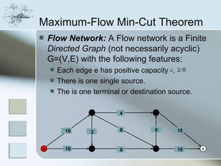
Maximum-Flow Min-Cut Theorem
 Flow Network: A Flow network is a Finite
Directed Graph (not necessarily acyclic)
G=(V,E) with the following features:
 Each edge e has positive capacity ce ≥ 0
 There is one single source.
 The is one terminal or destination source.

2 4 4

10 2 8 6 10

s 10 3 9 5 10 t

 Flow Function: S-t Flow function is f:ER which has the
following properties:
 It must be positive and should not exceed the capacity of each
edge.
0 ≤ f (e) ≤ ce
 ٍٍFor each node except for s and t sum of the input flow must be
equal to some of the output flow (Physical Law: ex. Information
Conservation).
∀v ∈ V - {s, t} ∑ f ( e) = ∑ f ( e )
e into v e out of v

 Flow Value: amount of information that enters into destination
node.
3 flow
2 4 4

5 2 3 capacity
10 2 0 8 6 0 10

7 7 9
s 10 3 9 5 10 t

Flow value = 12

 Question1: What is the maximum amount of information flow
achievable in this network?
 First Attempt: Using LP to compute the amount in polynomial
time (if integer valued are allowed it will be NP-Hard).
 Second Attempt: Heuristic Methods
 Algorithm(G,s,t)
Assign the initial flow to zero.
 For every simple path from s to t in Graph G
(Greedily) push positive flow on with respect to constraints.
 update the flow.

20/20 10/10
20/20 0/10
S 10/30 D
S 20/30 D
10/10 20/20
0/10 20/20
Flow Value = 30
Flow Value = 20
=Max Flow

 But How can we correct the previous algorithm?
 Suppose we made push forward in one path but
maybe our choice was not suitable so we put it on
mind and write the reverse path.
 With collecting this information, we get the second
graph which is called Residual Graph.
Graph

G: Gf:

0/10 20 10
20/20
20/30 S 10 20 D
S D

0/10 20/20 10 20

 So we can edit the previous algorithm
as below:
 Ford-Fulkerson Method (G,s,t):
 Start with zero flow.
 While there is a simple path between source and
destination in residual graph Gf :
 Push flow in it and update the flow function.

 Lets consider one example
graphically:

0 flow
2 4 4

G: 0 0 0 capacity
10 2 0 8 6 0 10

0 0 0
s 10 3 9 5 10 t

Flow value = 0

2 4 4
residual
Gf: capacity
10 2 8 6 10

s 10 3 9 5 10 t

0
2 4 4

G: 10 X
8 8 0
10 2 X
0 8 6 0 10
2
0 X 2
0 10 X
8
s 10 3 9 5 10 t

Flow value = 8

2 4 4

Gf: 8
2 2 8 6 10

s 10 3 9 5 2 t

8

0
2 4 4

G: 10 8 0
X 6
10 2 2 8 6X
0 10
6
X 6
0 X 8
2 10
s 10 3 9 5 10 t

Flow value = 10

2 4 4

Gf:
10 2 8 6 10

s 10 3 7 5 10 t

2

0
X 2
2 4 4

G: 10 8 6
X 8
10 2 X
2 8 6 6 10
0
X 8
6 8 10
s 10 3 9 5 10 t

Flow value = 16

2 4 4

Gf: 6
10 2 8 6 4

s 4 3 1 5 10 t
6 8

2
X 3
2 4 4

G: 10 X 7
8 8
X 9
10 2 0 8 6 6 10

X 9
8 X 9
8 10
s 10 3 9 5 10 t

Flow value = 18
2
2 2 4

Gf: 8
10 2 8 6 2

s 2 3 1 5 10 t
8 8

3
2 4 4

G: 10 7 9
10 2 0 8 6 6 10

9 9 10
s 10 3 9 5 10 t

Flow value = 19
3
2 1 4

Gf: 9
1
10 2 7 6 1

s 1 3 9 5 10 t
9

 Cut: s-t cut is a portion of the vertex set V
into sets A and B such:
s∈ A , t∈ B
A∪ B = V , A∩ B = φ

 Cut Capacity: The capacity of and s-t cut
denoted by :
c( A, B ) = ∑c
e out of A
e

 And finally we have the famous Max-Flow Min-
Cut Theorem:
 Max-Flow Min-Cut Theorem:

In every flow network the Ford-Fulkerson
method Reaches the graph maximum flow
and it is equal to minimum cut capacity.

 There are several Polynomial Time Algorithms
suggested for this problem. The following table
shows some of the famous ones.

Network Information Processing

So we can reach the maximum
information transferring with
routing (only with forwarding)
in polynomial time in Unicast
Scenario.

Maximum Information
Transferring in
Multicasting Scenario

 What is the maximum amount of
information that could be transferred in
multicasting scenario?
 The following graph shows the basic idea
for multicasting.

∞
Insert super node
and use max-Flow Super Terminal
Min-Cut Theorem.
∞

 So we can not exceed this bound.
 Now another question arises:

How can we make much more diversity of
independent packets in each
destination?

Simple Routing with Forwarding

Routing with Duplicate and Forward Packet Duplication

Lesson That we have learned:


With the usage of some functions in
each routing node, we could get
much more diversity of information
in each terminal nodes.

Duplicate Duplicate

Routing with Addition R+B
and Subtraction

Duplicate

B, R
R+B R+B

 In general we can model this technique as
below (Linear Operation):
Operation
x
a
y  x
α 11 α 12 α 13  α 11 α 12 α 13     a 
 ×  y = b
α 
 21 α 22 α 23 
α α α 23 
 21 22  z  
 
b
z

 Note that one can not achieve more that
max flow for each terminal (Upper Bound).

 The previous technique is divided into
two categories:
 Duplicate and Forward (Routing).
 Network Coding.
 The first strategy is something that is
used in current networking
technology.
 The second one may be used in near
future.

Duplicate and Forward
Sterategy

 It is obvious that if we let duplication a
packet path would be tree in DAG graph.
 So we could formulate follows:
Γ = {τ1 ,τ 2 ,τ 3 ,...,τ max } which each τi is routed
at Source Node,
f : Γ → ℜ+ ( Ζ+ )
f (τ i ) is define as flow on each τi .
D = { d1 , d 2 ,..., d max } which D is the set of
destinations or terminals.
E = {e1 , e2 ,..., emax } which E is the set of edges.
δ d ij = 1 ⇔ d i ∈τ j .
δ e ij = 1 ⇔ ei ∈τ j .
Packing Trees for getting Maximum Throughput
in each terminal node.
max ∑∑ f (τ
τ
d i ∈D
j ) ×δ d ij
j∈Γ

s.t :
∀τi ∈Γ, ∀e ∈E ∑∑ f (τ ) ×δ
τ
i
e
ij ≤ ce .
i ∈ ei ∈
Γ E

 There are some points about this
formulation.
 Generally the number of trees are exponential
according to the size of input graph.
 If we consider only integer values it will be
Linear Integer Programming.
 So where is the exact location of the tree
packing problem in polynomial time
hierarchy?
 It can be proved that this problem is NP-
Hard.

 So it seems that in general the
problem is hard.
 Let’s simplify the problem a bit to see
if it will be traceable.
 Lets assume that we want to pack
tree in a way that all of the terminals
get the same number of colors.
 It is obvious that the number of colors
could not exceed than min max-flow
(s,T).

 Unfortunately this version again is not
traceable.
 It is equal to Packing Steiner Trees which is
NP-Hard.
Generally there is no Polynomial Time
Algorithms that we could optimally
transfer packets with only Duplicate and
Forward strategy in Multicasting (P≠NP).
 Now if we empower each node with
complete linear operation what will happen?
(switching to network coding).

Linear Network Coding
In Multicasting

 We are working in GF(2q) field and
assuming each packet is in this field.
 All mathematical calculation is valid like
real number field.
 Just like previous session we assume that
the graph is DAG.
 There is no delay in each node for
scrambling inputs to make outputs.
 For Inputs we use X variable, for
intermediate Nodes Y and for the output
signals to be recovered, Z.

Type of nodes and their input-output relation

x1 y(e1)  α1e1 . α ne1   x1   y (e1 ) 
x2  . . .  × .  =  . 
     
y(em) α1em . α1em  m×n  xn  n×1  y (em ) m×1
     
xn

y(e*1) y(e1)  β e* e1 . β e* e1   y (e*1 )   y (e1 ) 
 1   
= . 
n

y(e*2) y(em)  . . .  × .   
β *   y (e * n )   y (em ) m×1
y(e*n)  e 1em . β e*nem  m× n   n×1  

y(e1)
z1
ε e1,1 . ε em ,1   y (e1 )   z1 
 
y(e2)  . . .  × .  =  . 
zn ε e1,n . ε em,n 
   
  n×m  y (em ) m×1  zn  n×1
   
y(em)

e1

v2
x1 e5
z1
e2
x2 v1 e4
v4 z2
e6
x3 e3 z3 It seems that each
v3 edge plays much
e7 important rule
than nodes so we

Conversion
convert the original
to the new graph
which each node
e5 stands as the edge
of the previous one.
e1
x1 z1

e4
x2 e2
z2

e6
x3
e3 z3

e7

e5 εe5,1
βe1,e5
α1,e1 e1 εe5,2
εe5,3
x1 α1,e2 βe1,e4 z1
α1,e3 βe2,e5
α2,e1 e4
α2,e2 e2
x2 βe2,e4 βe4,e6
α3,e2 z2
α3,e1 βe4,e7 εe6,1 εe6,2
α2,e3 e6
x3 βe3,e6 εe6,3
α3,e3 e3 εe7,2 z3
εe7,1
βe3,e7 εe7,3
e7

Output Matrix:
Internal Matrix: 0 0 0 0 εe 5,1 εe 6,1 εe 7 ,1 
 
B = 0 0 0 0 εe 5, 2 εe 6, 2 εe 7 , 2 
0 0 0 β e1,e 4 β e1,e5 0 0  0
 0 0 0 ε e 5, 3 εe 6 , 3 εe 7 , 3 

0 0 0 β e 2 ,e 4 β e 2 ,e 5 0 0 
 
0 0 0 0 0 β e 3, e 6 β e 3, e 7 

F = 0 0 0 0 0 β e 4,e 6

β e 4 ,e 7  Input Matrix:
0 0 0 0 0 0 0 
 
0 0 0 0 0 0 0  α1,e1 α1,e 2 α1,e 3 0 0 0 0
0  
 0 0 0 0 0 0   A = α 2,e1 α 2,e 2 α 2,e 3 0 0 0 0
α 3,e1 α 3,e 2 α 3,e 3
 0 0 0 0


 Question: How we can relate inputs and
outputs using these Matrices?
 It is obvious that A shows the inputs inject into
the network and the same, B shows that how
network information inject into outputs.
 How can we get the propagation in the
network?
 We must find all walk between source
edges and output edges.
 It can be proved easily, according to some
algebraic graph theory algorithms that:

  ∞
i T
z = x × A×  ∑ F × B 
  i =0  

 We can simplify the previous equation by the
following assumption.
 If we make the graph in topological order then we will
get the simpler equation:

z = x × A× ( I − F ) × B
−1 T

 And finally with some more challenges with have
the famous network coding theorem:

Consider a DAG G with unit capacities
that has a single source node s (with h
sources) and a set of terminal nodes T.
The multicast property with rate h is said
to be satisfied if max-Flow (s,Ti) ≥ h for
all Ti. If G satisfied the multicast property
a network code that supports the
multicast rate h is guaranteed to exist as
long as the field size is larger than |T |.

 So if the field size is large enough there
always exists network coding scheme that
reaches the limit.
 The are some polynomial time algorithms
suggested for making network codes, for
example LIF and Randomized Network
Coding Algorithms.
 For some special graphs with network
coding we could reach the maximum flow
for each node.
 So in summary we have:

With network coding we can
reach the maximum throughput
in polynomial time.

Comparison between two
methods in Multicasting
Scenario

 What is the theoretical Gap between
Network Coding and Routing?
 It can be proved that if the graph is
directed the gap is very large
(Ω(logn): where n is the number of
terminals).
 But if the graph is not directed the
gap is in the order of constant
number.

Network Coding Example
Suppose the following Directed Graph: Gha,b

 Lemma: Under routing the capacity of
the Gh2h,C(2h,h) is less than 2.
 with network coding the capacity of the
network could be h.
 with some error control coding codes
we can get the maximum capacity for
network coding.
 Example Reed-Solomon Codes:

Re ed − Solomon R ( n, k ) ::
→
M 1×k = [ M 0 , M 1 ,..., M k −1 ]
{α1 , α2 ,..., αn } ∈ GF (q) , ∀αi ≠ 0.
→
C1×n = [C0 , C1 ,..., Cn −1 ]
 1 1 ... 1 
 
→ →
 α1 α2 ... α n 
C 1×n = M 1×k 
. . ... . 
 k −1 
α 1 α k −12 k −1 
... α n 


The structure of the above matrix is Vandermonde
And with any h subset of the Codeword we can make
the original message.

 So in the source node we can use
RS(a,h) and in the terminals the
original signal can be made.
 This concept is sometimes categorized
as the source coding.

Maximum Information
Transferring in
Broadcasting Scenario

 In Broadcasting according to the
Edmond’s paper we can always pack
k- edge disjoint spanning trees where
k=min max-flow (s,Ti).
 So in this scenario, routing with
duplication has the same power as
network coding in general case.

Conclusion
 The basics of routing and its theoretical bounds
are reviewed.
 The basics of network coding and its theoretical
bounds are reviewed.
 It seems that in general network coding gives us
much more throughput, but contains more
computational complexity than general routing.

Unicast Multicast Broadcast
Network The same as each The performance of The same as each
Coding, other. Network Coding is other.
Routing much better and to
use routing we face
NP-Hard Problem.

Network Information Processing

Recommended

More Related Content

What's hot (20)

Viewers also liked (16)

Similar to Network Information Processing (20)

More from Reza Rahimi (18)

Recently uploaded (20)

Network Information Processing