A superglue for string comparison
0 likes448 views

The document describes string comparison techniques using matrix algebra and seaweed matrices. It introduces the concept of semi-local string comparison, which involves comparing a whole string to substrings of another string. The key idea is representing string comparison matrices implicitly using seaweed matrices, which represent unit-Monge matrices. This allows developing algebraic techniques for efficiently multiplying such matrices using the algebra of braids and the seaweed monoid. These multiplication techniques can then be applied to problems like dynamic programming string comparison and comparing compressed strings.


![Introduction
Implicit unit-Monge matrices
Efficient PΣ queries: range tree on nonzeros of P [Bentley: 1980]
binary search tree by i-coordinate
under every node, binary search tree by j-coordinate
•
•
•
•
−→ •
•
•
•
−→ •
•
•
•
↓
•
•
•
•
−→ •
•
•
•
−→ •
•
•
•
↓
•
•
•
•
−→ •
•
•
•
−→ •
•
•
•
Alexander Tiskin (Warwick) Semi-local LCS 12 / 164](https://image.slidesharecdn.com/tiskinalexandr-160927175041/85/A-superglue-for-string-comparison-18-320.jpg)

![Introduction
Implicit unit-Monge matrices
Efficient PΣ queries: (contd.)
Every node of the range tree represents a canonical range (rectangular
region), and stores its nonzero count
Overall, ≤ n log n canonical ranges are non-empty
A PΣ query is equivalent to -dominance counting: how many nonzeros
are -dominated by query point?
Answer: sum up nonzero counts in ≤ log2
n disjoint canonical ranges
Total size O(n log n), query time O(log2
n)
There are asymptotically more efficient (but less practical) data structures
Total size O(n), query time O log n
log log n [J´aJ´a+: 2004]
[Chan, Pˇatra¸scu: 2010]
Alexander Tiskin (Warwick) Semi-local LCS 13 / 164](https://image.slidesharecdn.com/tiskinalexandr-160927175041/85/A-superglue-for-string-comparison-20-320.jpg)


![Matrix distance multiplication
Seaweed matrix multiplication
Seaweed matrix -multiplication
Given permutation matrices P, Q, compute R, such that PΣ QΣ = RΣ
(equivalently, P Q = R)
Seaweed matrix -multiplication: running time
type time
general O(n3) standard
O n3(log log n)3
log2
n
[Chan: 2007]
Monge O(n2) via [Aggarwal+: 1987]
implicit unit-Monge O(n1.5) [T: 2006]
O(n log n) [T: 2010]
Alexander Tiskin (Warwick) Semi-local LCS 22 / 164](https://image.slidesharecdn.com/tiskinalexandr-160927175041/85/A-superglue-for-string-comparison-36-320.jpg)


![Matrix distance multiplication
Bruhat order
Bruhat comparability: running time
O(n2) [Ehresmann: 1934; Proctor: 1982; Grigoriev: 1982]
O(n log n) [T: 2013]
O n log n
log log n [Gawrychowski: NEW]
Alexander Tiskin (Warwick) Semi-local LCS 29 / 164](https://image.slidesharecdn.com/tiskinalexandr-160927175041/85/A-superglue-for-string-comparison-49-320.jpg)


![Matrix distance multiplication
Bruhat order
Alternative solution: clever implementation of Ehresmann’s criterion
[Gawrychowski: 2013]
The online partial sums problem: maintain array X[1 : n], subject to
update(k, ∆): X[k] ← X[k] + ∆
prefixsum(k): return 1≤i≤k X[i]
Query time:
Θ(log n) in semigroup or group model
Θ log n
log log n in RAM model on integers [Pˇatra¸scu, Demaine: 2004]
Gives Bruhat comparability in time O n log n
log log n in RAM model
Open problem: seaweed multiplication in time O n log n
log log n ?
Alexander Tiskin (Warwick) Semi-local LCS 34 / 164](https://image.slidesharecdn.com/tiskinalexandr-160927175041/85/A-superglue-for-string-comparison-60-320.jpg)


![Semi-local string comparison
Semi-local LCS and edit distance
The LCS problem
Give the LCS score for a vs b
LCS: running time
O(mn) [Wagner, Fischer: 1974]
O mn
log2
n
σ = O(1) [Masek, Paterson: 1980]
[Crochemore+: 2003]
O mn(log log n)2
log2
n
[Paterson, Danˇc´ık: 1994]
[Bille, Farach-Colton: 2008]
Running time varies depending on the RAM model version
We assume word-RAM with word size log n (where it matters)
Alexander Tiskin (Warwick) Semi-local LCS 37 / 164](https://image.slidesharecdn.com/tiskinalexandr-160927175041/85/A-superglue-for-string-comparison-65-320.jpg)


![Semi-local string comparison
Semi-local LCS and edit distance
LCS: dynamic programming [WF: 1974]
Sweep cells in any -compatible order
Cell update: time O(1)
Overall time O(mn)
Alexander Tiskin (Warwick) Semi-local LCS 40 / 164](https://image.slidesharecdn.com/tiskinalexandr-160927175041/85/A-superglue-for-string-comparison-80-320.jpg)
![Semi-local string comparison
Semi-local LCS and edit distance
LCS: micro-block dynamic programming [MP: 1980; BF: 2008]
Sweep cells in micro-blocks, in any -compatible order
Micro-block size:
t = O(log n) when σ = O(1)
t = O log n
log log n otherwise
Micro-block interface:
O(t) characters, each O(log σ) bits, can be reduced to O(log t) bits
O(t) small integers, each O(1) bits
Micro-block update: time O(1), by precomputing all possible interfaces
Overall time O mn
log2
n
when σ = O(1), O mn(log log n)2
log2
n
otherwise
Alexander Tiskin (Warwick) Semi-local LCS 41 / 164](https://image.slidesharecdn.com/tiskinalexandr-160927175041/85/A-superglue-for-string-comparison-81-320.jpg)


![Semi-local string comparison
Score matrices and seaweed matrices
Semi-local LCS: output representation and running time
size query time
O(n2) O(1) trivial
O(m1/2n) O(log n) string-substring [Alves+: 2003]
O(n) O(n) string-substring [Alves+: 2005]
O(n log n) O(log2
n) [T: 2006]
. . . or any 2D orthogonal range counting data structure
running time
O(mn2) naive
O(mn) string-substring [Schmidt: 1998; Alves+: 2005]
O(mn) [T: 2006]
O mn
log0.5
n
[T: 2006]
O mn(log log n)2
log2
n
[T: 2007]
Alexander Tiskin (Warwick) Semi-local LCS 47 / 164](https://image.slidesharecdn.com/tiskinalexandr-160927175041/85/A-superglue-for-string-comparison-89-320.jpg)


![The seaweed method
Seaweed combing
Semi-local LCS: seaweed combing [T: 2006]
Initialise uncombed seaweed braid: mismatch cell = crossing
Sweep cells in any -compatible order
match cell: skip (keep uncrossed)
mismatch cell: comb (uncross) iff the same seaweed pair already
crossed before
Cell update: time O(1)
Overall time O(mn)
Correctness: by seaweed monoid relations
Alexander Tiskin (Warwick) Semi-local LCS 61 / 164](https://image.slidesharecdn.com/tiskinalexandr-160927175041/85/A-superglue-for-string-comparison-144-320.jpg)


![The seaweed method
Micro-block seaweed combing
Semi-local LCS: micro-block seaweed combing [T: 2007]
Initialise uncombed seaweed braid: mismatch cell = crossing
Sweep cells in micro-blocks, in any -compatible order
Micro-block size: t = O log n
log log n
Micro-block interface:
O(t) characters, each O(log σ) bits, can be reduced to O(log t) bits
O(t) integers, each O(log n) bits, can be reduced to O(log t) bits
Micro-block update: time O(1), by precomputing all possible interfaces
Overall time O mn(log log n)2
log2
n
Alexander Tiskin (Warwick) Semi-local LCS 65 / 164](https://image.slidesharecdn.com/tiskinalexandr-160927175041/85/A-superglue-for-string-comparison-160-320.jpg)

![The seaweed method
Cyclic LCS
The cyclic LCS problem
Give the maximum LCS score for a vs all cyclic rotations of b
Cyclic LCS: running time
O mn2
log n naive
O(mn log m) [Maes: 1990]
O(mn) [Bunke, B¨uhler: 1993; Landau+: 1998; Schmidt: 1998]
O mn(log log n)2
log2
n
[T: 2007]
Alexander Tiskin (Warwick) Semi-local LCS 66 / 164](https://image.slidesharecdn.com/tiskinalexandr-160927175041/85/A-superglue-for-string-comparison-162-320.jpg)


![The seaweed method
Longest repeating subsequence
The longest repeating subsequence problem
Find the longest subsequence of a that is a square (a repetition of two
identical strings)
Longest repeating subsequence: running time
O(m3) naive
O(m2) [Kosowski: 2004]
O m2(log log m)2
log2
m
[T: 2007]
Alexander Tiskin (Warwick) Semi-local LCS 68 / 164](https://image.slidesharecdn.com/tiskinalexandr-160927175041/85/A-superglue-for-string-comparison-165-320.jpg)

![The seaweed method
Approximate matching
The approximate pattern matching problem
Give the substring closest to a by alignment score, starting at each
position in b
Assume rational scoring scheme
Approximate pattern matching: running time
O(mn) [Sellers: 1980]
O mn
log n σ = O(1) via [Masek, Paterson: 1980]
O mn(log log n)2
log2
n
via [Bille, Farach-Colton: 2008]
Alexander Tiskin (Warwick) Semi-local LCS 70 / 164](https://image.slidesharecdn.com/tiskinalexandr-160927175041/85/A-superglue-for-string-comparison-167-320.jpg)
![The seaweed method
Approximate matching
Approximate pattern matching: the algorithm
Micro-block seaweed combing on a vs b (with blow-up), time
O mn(log log n)2
log2
n
The implicit semi-local edit score matrix:
an anti-Monge matrix
approximate pattern matching ∼ row minima
Row minima in O(n) element queries [Aggarwal+: 1987]
Each query in time O(log2
n) using the range tree representation,
combined query time negligible
Overall running time O mn(log log n)2
log2
n
, same as [Bille, Farach-Colton: 2008]
Alexander Tiskin (Warwick) Semi-local LCS 71 / 164](https://image.slidesharecdn.com/tiskinalexandr-160927175041/85/A-superglue-for-string-comparison-168-320.jpg)


![Periodic string comparison
Wraparound seaweed combing
The tandem LCS problem
Give LCS score for a vs b = uk
We have n = kp; may assume k ≤ m
Tandem LCS: running time
O(mkp) naive
O m(k + p) [Landau, Ziv-Ukelson: 2001]
O(mp) [T: 2009]
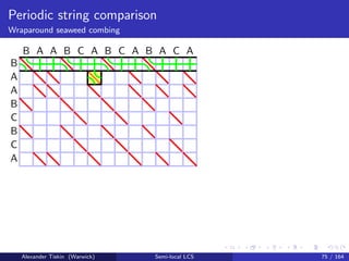
Direct application of wraparound seaweed combing
Alexander Tiskin (Warwick) Semi-local LCS 78 / 164](https://image.slidesharecdn.com/tiskinalexandr-160927175041/85/A-superglue-for-string-comparison-214-320.jpg)
![Periodic string comparison
Wraparound seaweed combing
The tandem alignment problem
Give the substring closest to a in b = u±∞ by alignment score among
global: substrings uk of length kp across all k
cyclic: substrings of length kp across all k
local: substrings of any length
Tandem alignment: running time
O(m2p) all naive
O(mp) global [Myers, Miller: 1989]
O(mp log p) cyclic [Benson: 2005]
O(mp) cyclic [T: 2009]
O(mp) local [Myers, Miller: 1989]
Alexander Tiskin (Warwick) Semi-local LCS 79 / 164](https://image.slidesharecdn.com/tiskinalexandr-160927175041/85/A-superglue-for-string-comparison-215-320.jpg)
![Periodic string comparison
Wraparound seaweed combing
Cyclic tandem alignment: the algorithm
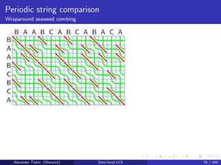
Periodic seaweed combing for a vs b (with blow-up), time O(mp)
For each k ∈ [1 : m]:
solve tandem LCS (under given alignment score) for a vs uk
obtain scores for a vs p successive substrings of b of length kp by LCS
batch query: time O(1) per substring
Running time O(mp)
Alexander Tiskin (Warwick) Semi-local LCS 80 / 164](https://image.slidesharecdn.com/tiskinalexandr-160927175041/85/A-superglue-for-string-comparison-216-320.jpg)

![Sparse string comparison
Semi-local LCS between permutations
The LCS problem on permutation strings (LCSP)
Give LCS score for a vs b; in each of a, b all characters distinct
Equivalent to
longest increasing subsequence (LIS) in a string
maximum clique in a permutation graph
maximum planar matching in an embedded bipartite graph
LCSP: running time
O(n log n) implicit in [Erd¨os, Szekeres: 1935]
[Robinson: 1938; Knuth: 1970; Dijkstra: 1980]
O(n log log n) unit-RAM [Chang, Wang: 1992]
[Bespamyatnikh, Segal: 2000]
Alexander Tiskin (Warwick) Semi-local LCS 82 / 164](https://image.slidesharecdn.com/tiskinalexandr-160927175041/85/A-superglue-for-string-comparison-218-320.jpg)
![Sparse string comparison
Semi-local LCS between permutations
Semi-local LCSP
Give semi-local LCS scores for a vs b; in each of a, b all characters distinct
Equivalent to
longest increasing subsequence (LIS) in every substring of a string
Semi-local LCSP: running time
O(n2 log n) naive
O(n2) restricted [Albert+: 2003; Chen+: 2005]
O(n1.5 log n) randomised, restricted [Albert+: 2007]
O(n1.5) [T: 2006]
O(n log2
n) [T: 2010]
Alexander Tiskin (Warwick) Semi-local LCS 83 / 164](https://image.slidesharecdn.com/tiskinalexandr-160927175041/85/A-superglue-for-string-comparison-219-320.jpg)


![Sparse string comparison
Longest piecewise monotone subsequences
A k-increasing sequence: a concatenation of k increasing sequences
A (k − 1)-modal sequence: a concatenation of k alternating increasing and
decreasing sequences
The longest k-increasing (or (k − 1)-modal) subsequence problem
Give the longest k-increasing ((k − 1)-modal) subsequence of string b
Longest k-increasing (or (k − 1)-modal) subsequence: running time
O(nk log n) (k − 1)-modal [Demange+: 2007]
O(nk log n) via [Hunt, Szymanski: 1977]
O(n log2
n) [T: 2010]
Main idea: lcs(idk
, b) (respectively, lcs((idid)k/2, b))
Alexander Tiskin (Warwick) Semi-local LCS 89 / 164](https://image.slidesharecdn.com/tiskinalexandr-160927175041/85/A-superglue-for-string-comparison-225-320.jpg)


![Sparse string comparison
Maximum clique in a circle graph
Maximum clique in a circle graph: running time
exp(n) naive
O(n3) [Gavril: 1973]
O(n2) [Rotem, Urrutia: 1981; Hsu: 1985]
[Masuda+: 1990; Apostolico+: 1992]
O(n1.5) [T: 2006]
O(n log2
n) [T: 2010]
Alexander Tiskin (Warwick) Semi-local LCS 92 / 164](https://image.slidesharecdn.com/tiskinalexandr-160927175041/85/A-superglue-for-string-comparison-230-320.jpg)


![Sparse string comparison
Maximum clique in a circle graph
Parameterised maximum clique in a circle graph
The maximum clique problem in a circle graph, sensitive e.g. to
number e of edges; e ≤ n2
size l of maximum clique; l ≤ n
cutwidth d of interval model (max number of intervals covering a
point); l ≤ d ≤ n
Parameterised maximum clique in a circle graph: running time
O(n log n + e) [Apostolico+: 1992]
O(n log n + nl log(n/l)) [Apostolico+: 1992]
O(n log n + n log2
d) NEW
Alexander Tiskin (Warwick) Semi-local LCS 95 / 164](https://image.slidesharecdn.com/tiskinalexandr-160927175041/85/A-superglue-for-string-comparison-243-320.jpg)


![Compressed string comparison
Extended substring-string LCS on GC-strings
LCS: running time (r = m + n, ¯r = ¯m + ¯n)
p t
plain plain O(mn) [Wagner, Fischer: 1974]
O mn
log2
m
[Masek, Paterson: 1980]
[Crochemore+: 2003]
plain GC O(m3 ¯n + . . .) gen. CFG [Myers: 1995]
O(m1.5 ¯n) ext subs-s [T: 2008]
O(m log m · ¯n) ext subs-s [T: 2010]
GC GC NP-hard [Lifshits: 2005]
O(r1.2¯r1.4) R weights [Hermelin+: 2009]
O(r log r · ¯r) [T: 2010]
O r log(r/¯r) · ¯r [Hermelin+: 2010]
O r log1/2
(r/¯r) · ¯r [Gawrychowski: 2012]
Alexander Tiskin (Warwick) Semi-local LCS 100 / 164](https://image.slidesharecdn.com/tiskinalexandr-160927175041/85/A-superglue-for-string-comparison-248-320.jpg)

![Compressed string comparison
Subsequence recognition on GC-strings
The global subsequence recognition problem
Does pattern p appear in text t as a subsequence?
Global subsequence recognition: running time
p t
plain plain O(n) greedy
plain GC O(m¯n) greedy
GC GC NP-hard [Lifshits: 2005]
Alexander Tiskin (Warwick) Semi-local LCS 102 / 164](https://image.slidesharecdn.com/tiskinalexandr-160927175041/85/A-superglue-for-string-comparison-250-320.jpg)

![Compressed string comparison
Subsequence recognition on GC-strings
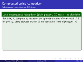
Local subsequence recognition: running time ( + output)
p t
plain plain O(mn) [Mannila+: 1995]
O mn
log m [Das+: 1997]
O(cm + n) [Boasson+: 2001]
O(m + nσ) [Troniˇcek: 2001]
plain GC O(m2 log m¯n) [C´egielski+: 2006]
O(m1.5 ¯n) [T: 2008]
O(m log m · ¯n) [T: 2010]
O(m · ¯n) [Yamamoto+: 2011]
GC GC NP-hard [Lifshits: 2005]
Alexander Tiskin (Warwick) Semi-local LCS 104 / 164](https://image.slidesharecdn.com/tiskinalexandr-160927175041/85/A-superglue-for-string-comparison-252-320.jpg)
![Compressed string comparison
Subsequence recognition on GC-strings
ˆı0+ ˆı1+ ˆı2+
ˆ0+ ˆ1+ ˆ2+
0 n n
b i : j matching iff box [i : j] not pierced left-to-right
Determined by -chain of -maximal seaweeds
b i : j minimally matching iff (i, j) is in the interleaved skeleton -chain
Alexander Tiskin (Warwick) Semi-local LCS 105 / 164](https://image.slidesharecdn.com/tiskinalexandr-160927175041/85/A-superglue-for-string-comparison-253-320.jpg)


![Compressed string comparison
Threshold approximate matching
Threshold approximate matching: running time ( + output)
p t
plain plain O(mn) [Sellers: 1980]
O(mk) [Landau, Vishkin: 1989]
O(m + n + nk4
m ) [Cole, Hariharan: 2002]
plain GC O(m¯nk2) [K¨arkk¨ainen+: 2003]
O(m¯nk + ¯n log n) [LV: 1989] via [Bille+: 2010]
O(m¯n + ¯nk4 + ¯n log n) [CH: 2002] via [Bille+: 2010]
O(m log m · ¯n) [T: NEW]
GC GC NP-hard [Lifshits: 2005]
(Also many specialised variants for LZ compression)
Alexander Tiskin (Warwick) Semi-local LCS 109 / 164](https://image.slidesharecdn.com/tiskinalexandr-160927175041/85/A-superglue-for-string-comparison-259-320.jpg)


![Compressed string comparison
Threshold approximate matching
Threshold approx matching (plain pattern, GC text): the algorithm
Algorithm structure similar to local subsequence recognition
-chains replaced by m × m submatrices
Extra ingredients:
the blow-up technique: reduction of edit distances to LCS scores
implicit matrix searching, replaces -chain interleaving
Monge row minima: “SMAWK” O(m) [Aggarwal+: 1987]
Implicit unit-Monge row minima:
O(m log log m) [T: 2012]
O(m) [Gawrychowski: 2012]
Overall time O(m log m · ¯n) + O(m¯n) = O(m log m · ¯n)
Alexander Tiskin (Warwick) Semi-local LCS 112 / 164](https://image.slidesharecdn.com/tiskinalexandr-160927175041/85/A-superglue-for-string-comparison-262-320.jpg)

![Parallel string comparison
Parallel LCS
Bulk-Synchronous Parallel (BSP) computer [Valiant: 1990]
Simple, realistic general-purpose parallel
model
COMM. ENV . (g, l)
0
P
M
1
P
M
p − 1
P
M· · ·
Alexander Tiskin (Warwick) Semi-local LCS 114 / 164](https://image.slidesharecdn.com/tiskinalexandr-160927175041/85/A-superglue-for-string-comparison-264-320.jpg)
![Parallel string comparison
Parallel LCS
Bulk-Synchronous Parallel (BSP) computer [Valiant: 1990]
Simple, realistic general-purpose parallel
model
COMM. ENV . (g, l)
0
P
M
1
P
M
p − 1
P
M· · ·
Contains
p processors, each with local memory (1 time unit/operation)
communication environment, including a network and an external
memory (g time units/data unit communicated)
barrier synchronisation mechanism (l time units/synchronisation)
Alexander Tiskin (Warwick) Semi-local LCS 114 / 164](https://image.slidesharecdn.com/tiskinalexandr-160927175041/85/A-superglue-for-string-comparison-265-320.jpg)


![Parallel string comparison
Parallel LCS
BSP software: industrial projects
Google’s Pregel [2010]
Apache Spark (hama.apache.org) [2010]
Apache Giraph (giraph.apache.org) [2011]
BSP software: research projects
Oxford BSP (www.bsp-worldwide.org/implmnts/oxtool) [1998]
Paderborn PUB (www2.cs.uni-paderborn.de/~pub) [1998]
BSML (traclifo.univ-orleans.fr/BSML) [1998]
BSPonMPI (bsponmpi.sourceforge.net) [2006]
Multicore BSP (www.multicorebsp.com) [2011]
Epiphany BSP (www.codu.in/ebsp) [2015]
Petuum (petuum.org) [2015]
Alexander Tiskin (Warwick) Semi-local LCS 118 / 164](https://image.slidesharecdn.com/tiskinalexandr-160927175041/85/A-superglue-for-string-comparison-278-320.jpg)


![Parallel string comparison
Parallel LCS
Parallel LCS computation (cont.)
Parallel semi-local LCS: running time, comm, sync
comp comm sync
O(n2/p) O(n) O(p) 2D grid
O(n2/p) O n
p1/2 O(log2
p) [Krusche, T: 2007]
O n log p
p1/2 O(log p) [Krusche, T: 2010]
O n
p1/2 O(log p) [T: NEW]
Based on parallel Steady Ant algorithm
Alexander Tiskin (Warwick) Semi-local LCS 124 / 164](https://image.slidesharecdn.com/tiskinalexandr-160927175041/85/A-superglue-for-string-comparison-294-320.jpg)


![Parallel string comparison
Parallel LCS
Parallel LCS on permutation strings (LCSP = LIS)
Sequential time O(n log n), no good way known to parallelise directly
Solution via the more general semi-local LCSP is no longer efficient:
sequential time O(n log2
n)
Divide-and-conquer on substrings/subsequences of a, b
Parallelising normal O(n log n) seaweed multiplication: [Krusche, T: 2010]
comp O n log2
n
p comm O n log p
p sync O(log2
p)
Open problem: can we achieve
comp O n log n
p for LCSP?
comp O n log2
n
p , comm O(n
p ), sync O(log2
p) for semi-local LCSP?
Alexander Tiskin (Warwick) Semi-local LCS 129 / 164](https://image.slidesharecdn.com/tiskinalexandr-160927175041/85/A-superglue-for-string-comparison-299-320.jpg)

![The transposition network method
Transposition networks
Comparison network: a circuit of comparators
A comparator sorts two inputs and outputs them in prescribed order
Comparison networks traditionally used for non-branching merging/sorting
Classical comparison networks
# comparators
merging O(n log n) [Batcher: 1968]
sorting O(n log2
n) [Batcher: 1968]
O(n log n) [Ajtai+: 1983]
Alexander Tiskin (Warwick) Semi-local LCS 131 / 164](https://image.slidesharecdn.com/tiskinalexandr-160927175041/85/A-superglue-for-string-comparison-301-320.jpg)
![The transposition network method
Transposition networks
Comparison network: a circuit of comparators
A comparator sorts two inputs and outputs them in prescribed order
Comparison networks traditionally used for non-branching merging/sorting
Classical comparison networks
# comparators
merging O(n log n) [Batcher: 1968]
sorting O(n log2
n) [Batcher: 1968]
O(n log n) [Ajtai+: 1983]
Comparison networks are visualised by wire diagrams
Transposition network: all comparisons are between adjacent wires
Alexander Tiskin (Warwick) Semi-local LCS 131 / 164](https://image.slidesharecdn.com/tiskinalexandr-160927175041/85/A-superglue-for-string-comparison-302-320.jpg)


![The transposition network method
Parameterised string comparison
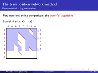
Parameterised string comparison: running time
Low-similarity, after preprocessing in O(n log σ)
O(nλ) [Hirschberg: 1977]
[Apostolico, Guerra: 1985]
[Apostolico+: 1992]
High-similarity, no preprocessing
O(n · κ) [Ukkonen: 1985]
[Myers: 1986]
Flexible
O(λ · κ · log n) no preproc [Myers: 1986; Wu+: 1990]
O(λ · κ) after preproc [Rick: 1995]
Alexander Tiskin (Warwick) Semi-local LCS 136 / 164](https://image.slidesharecdn.com/tiskinalexandr-160927175041/85/A-superglue-for-string-comparison-307-320.jpg)


![The transposition network method
Dynamic string comparison
Dynamic LCS in linear time: update models
left right
– app+del standard DP [Wagner, Fischer: 1974]
prep app a fixed [Landau+: 1998], [Kim, Park: 2004]
prep app [Ishida+: 2005]
prep+del app+del [T: NEW]
Dynamic semi-local LCS in linear time: update models
left right
prep+del app+del amortised [T: NEW]
Alexander Tiskin (Warwick) Semi-local LCS 139 / 164](https://image.slidesharecdn.com/tiskinalexandr-160927175041/85/A-superglue-for-string-comparison-332-320.jpg)
![The transposition network method
Bit-parallel string comparison
Bit-parallel string comparison
String comparison using standard instructions on words of size w
Bit-parallel string comparison: running time
O(mn/w) [Allison, Dix: 1986; Myers: 1999; Crochemore+: 2001]
Alexander Tiskin (Warwick) Semi-local LCS 140 / 164](https://image.slidesharecdn.com/tiskinalexandr-160927175041/85/A-superglue-for-string-comparison-333-320.jpg)


![Beyond semi-locality
Fixed-length substring LCS
Given window length w, let w-window be any substring of length w
The window-substring LCS problem
Give LCS score for every w-window of a vs every substring of b
Window-substring LCS: running time
O(mn3w) naive
O(mnw) multiple seaweed
O(mn) [Krusche, T: 2010]
Alexander Tiskin (Warwick) Semi-local LCS 145 / 164](https://image.slidesharecdn.com/tiskinalexandr-160927175041/85/A-superglue-for-string-comparison-340-320.jpg)


![Beyond semi-locality
Fixed-length substring LCS
The window-window LCS problem
Give LCS score for every w-window of a vs every w-window of b
Provides an LCS-scored alignment plot (by analogy with Hamming-scored
dot plot), a useful tool for studying weak conservation in the genome
Window-window LCS: running time
O(mnw2) naive
O(mnw) repeated seaweed combing
O(mn) [Krusche, T: 2010]
Alexander Tiskin (Warwick) Semi-local LCS 147 / 164](https://image.slidesharecdn.com/tiskinalexandr-160927175041/85/A-superglue-for-string-comparison-343-320.jpg)
![Beyond semi-locality
Fixed-length substring LCS
An implementation of alignment plots [Krusche: 2010]
Based on O(mnw) repeated seaweed combing approach, using some ideas
from the optimal O(mn) algorithm: resulting time O(mnw0.5)
Weighted alignment (match 1, mismatch 0, gap −0.5) via alignment dag
blow-up: ×4 slowdown
C++, Intel assembly (x86, x86 64, MMX/SSE2 data parallelism)
SMP parallelism (currently two processors)
Alexander Tiskin (Warwick) Semi-local LCS 148 / 164](https://image.slidesharecdn.com/tiskinalexandr-160927175041/85/A-superglue-for-string-comparison-344-320.jpg)


![Beyond semi-locality
Fixed-length substring LCS
Publications:
[Picot+: 2010] Evolutionary Analysis of Regulatory Sequences (EARS) in
Plants. Plant Journal.
[Baxter+: 2012] Conserved Noncoding Sequences Highlight Shared
Components of Regulatory Networks in Dicotyledonous Plants. Plant Cell.
Web service: http://wsbc.warwick.ac.uk/ears
Warwick press release (with video): http://www2.warwick.ac.uk/
newsandevents/pressreleases/discovery_of_100
Future work: genomic repeats; genome-scale comparison
Alexander Tiskin (Warwick) Semi-local LCS 153 / 164](https://image.slidesharecdn.com/tiskinalexandr-160927175041/85/A-superglue-for-string-comparison-349-320.jpg)

![Beyond semi-locality
Quasi-local LCS and spliced alignment
Given m (possibly overlapping) prescribed substrings in a
The quasi-local LCS problem
Give LCS score for every prescribed substring of a vs every subsring of b
Quasi-local LCS: running time
O(m2n) repeated seaweed combing
O(mn log2
m) [T: unpublished]
Alexander Tiskin (Warwick) Semi-local LCS 154 / 164](https://image.slidesharecdn.com/tiskinalexandr-160927175041/85/A-superglue-for-string-comparison-351-320.jpg)


![Beyond semi-locality
Quasi-local LCS and spliced alignment
The spliced alignment problem
Give the chain of non-overlapping prescribed substrings in a, closest to b
by alignment score
Describes gene assembly from candidate exons, given a known similar gene
Assume m = n; let s = total size of prescribed substrings
Spliced alignment: running time
O(ns) = O(n3) [Gelfand+: 1996]
O(n2.5) [Kent+: 2006]
O(n2 log2
n) [T: unpublished]
O(n2 log n) [Sakai: 2009]
Alexander Tiskin (Warwick) Semi-local LCS 156 / 164](https://image.slidesharecdn.com/tiskinalexandr-160927175041/85/A-superglue-for-string-comparison-354-320.jpg)
![Beyond semi-locality
Local alignment
Assume a fixed set of character alignment scores
The Smith–Waterman local alignment problem
For every prefix of a and every prefix of b, give a pair of respective suffixes
of these prefixes that have the highest alignment score against each other
Smith–Waterman local alignment: running time
O(m2n2) [naive]
O(mn) [Smith, Waterman: 1981]
Alexander Tiskin (Warwick) Semi-local LCS 157 / 164](https://image.slidesharecdn.com/tiskinalexandr-160927175041/85/A-superglue-for-string-comparison-355-320.jpg)
![Beyond semi-locality
Local alignment
Smith–Waterman local alignment [SW: 1981]
Sweep cells in any -compatible order
Cell update: time O(1)
Overall time O(mn)
Smith–Waterman local alignment maximises alignment score irrespective
of length
May not always be the most relevant alignment, e.g. may be
too short (would prefer a longer alignment even with a lower score)
too long (would prefer a significantly shorter alignment with slightly
lower score)
Alexander Tiskin (Warwick) Semi-local LCS 158 / 164](https://image.slidesharecdn.com/tiskinalexandr-160927175041/85/A-superglue-for-string-comparison-356-320.jpg)


A superglue for string comparison
- 1. A superglue for string comparison Alexander Tiskin Department of Computer Science, University of Warwick http://go.warwick.ac.uk/alextiskin Alexander Tiskin (Warwick) Semi-local LCS 1 / 164
- 2. 1 Introduction 2 Matrix distance multiplication 3 Semi-local string comparison 4 The seaweed method 5 Periodic string comparison 6 Sparse string comparison 7 Compressed string comparison 8 Parallel string comparison 9 The transposition network method 10 Beyond semi-locality Alexander Tiskin (Warwick) Semi-local LCS 2 / 164
- 3. 1 Introduction 2 Matrix distance multiplication 3 Semi-local string comparison 4 The seaweed method 5 Periodic string comparison 6 Sparse string comparison 7 Compressed string comparison 8 Parallel string comparison 9 The transposition network method 10 Beyond semi-locality Alexander Tiskin (Warwick) Semi-local LCS 3 / 164
- 4. Introduction String matching: finding an exact pattern in a string String comparison: finding similar patterns in two strings Alexander Tiskin (Warwick) Semi-local LCS 4 / 164
- 5. Introduction String matching: finding an exact pattern in a string String comparison: finding similar patterns in two strings global: whole string a vs whole string b semi-local: whole string a vs substrings in b (approximate matching); prefixes in a vs suffixes in b local: substrings in a vs substrings in b Alexander Tiskin (Warwick) Semi-local LCS 4 / 164
- 6. Introduction String matching: finding an exact pattern in a string String comparison: finding similar patterns in two strings global: whole string a vs whole string b semi-local: whole string a vs substrings in b (approximate matching); prefixes in a vs suffixes in b local: substrings in a vs substrings in b We focus on semi-local comparison: fundamentally important for both global and local comparison exciting mathematical properties Alexander Tiskin (Warwick) Semi-local LCS 4 / 164
- 7. Introduction Overview Standard approach to string comparison: dynamic programming Our approach: the algebra of seaweed matrices/braids Can be used either for dynamic programming, or for divide-and-conquer Divide-and-conquer is more efficient for: comparing dynamic strings (truncation, concatenation) comparing compressed strings (e.g. LZ-compression) comparing strings in parallel The “conquer” step involves a magic “superglue” (efficient multiplication of seaweed matrices/braids) Alexander Tiskin (Warwick) Semi-local LCS 5 / 164
- 8. Introduction Terminology and notation The “squared paper” notation: Integers {. . . − 2, −1, 0, 1, 2, . . .} x− = x − 1 2 x+ = x + 1 2 Half-integers . . . − 3 2, −1 2, 1 2, 3 2, 5 2, . . . = . . . (−2)+, (−1)+, 0+, 1+, 2+ Planar dominance: (i, j) (i , j ) iff i < i and j < j (the “above-left” relation) (i, j) (i , j ) iff i > i and j < j (the “below-left” relation) where “above/below” follow matrix convention (not the Cartesian one!) Alexander Tiskin (Warwick) Semi-local LCS 6 / 164
- 9. Introduction Terminology and notation A permutation matrix is a 0/1 matrix with exactly one nonzero per row and per column 0 1 0 1 0 0 0 0 1 Alexander Tiskin (Warwick) Semi-local LCS 7 / 164
- 10. Introduction Terminology and notation Given matrix D, its distribution matrix is made up of -dominance sums: DΣ(i, j) = ˆı>i,ˆ<j D(i, j) Alexander Tiskin (Warwick) Semi-local LCS 8 / 164
- 11. Introduction Terminology and notation Given matrix D, its distribution matrix is made up of -dominance sums: DΣ(i, j) = ˆı>i,ˆ<j D(i, j) Given matrix E, its density matrix is made up of quadrangle differences: E (ˆı, ˆ) = E(ˆı−, ˆ+) − E(ˆı−, ˆ−) − E(ˆı+, ˆ+) + E(ˆı+, ˆ−) where DΣ, E over integers; D, E over half-integers Alexander Tiskin (Warwick) Semi-local LCS 8 / 164
- 12. Introduction Terminology and notation Given matrix D, its distribution matrix is made up of -dominance sums: DΣ(i, j) = ˆı>i,ˆ<j D(i, j) Given matrix E, its density matrix is made up of quadrangle differences: E (ˆı, ˆ) = E(ˆı−, ˆ+) − E(ˆı−, ˆ−) − E(ˆı+, ˆ+) + E(ˆı+, ˆ−) where DΣ, E over integers; D, E over half-integers 0 1 0 1 0 0 0 0 1 Σ = 0 1 2 3 0 1 1 2 0 0 0 1 0 0 0 0 0 1 2 3 0 1 1 2 0 0 0 1 0 0 0 0 = 0 1 0 1 0 0 0 0 1 Alexander Tiskin (Warwick) Semi-local LCS 8 / 164
- 13. Introduction Terminology and notation Given matrix D, its distribution matrix is made up of -dominance sums: DΣ(i, j) = ˆı>i,ˆ<j D(i, j) Given matrix E, its density matrix is made up of quadrangle differences: E (ˆı, ˆ) = E(ˆı−, ˆ+) − E(ˆı−, ˆ−) − E(ˆı+, ˆ+) + E(ˆı+, ˆ−) where DΣ, E over integers; D, E over half-integers 0 1 0 1 0 0 0 0 1 Σ = 0 1 2 3 0 1 1 2 0 0 0 1 0 0 0 0 0 1 2 3 0 1 1 2 0 0 0 1 0 0 0 0 = 0 1 0 1 0 0 0 0 1 (DΣ) = D for all D Matrix E is simple, if (E )Σ = E; equivalently, if it has all zeros in the left column and bottom row Alexander Tiskin (Warwick) Semi-local LCS 8 / 164
- 14. Introduction Terminology and notation Matrix E is Monge, if E is nonnegative Intuition: boundary-to-boundary distances in a (weighted) planar graph G. Monge (1746–1818) G (planar) i j 0 1 2 3 4 0 1 2 3 4 Alexander Tiskin (Warwick) Semi-local LCS 9 / 164
- 15. Introduction Terminology and notation Matrix E is Monge, if E is nonnegative Intuition: boundary-to-boundary distances in a (weighted) planar graph G. Monge (1746–1818) i j 0 1 2 3 4 0 1 2 3 4 blue + blue ≤ red + red Alexander Tiskin (Warwick) Semi-local LCS 10 / 164
- 16. Introduction Terminology and notation Matrix E is unit-Monge, if E is a permutation matrix Intuition: boundary-to-boundary distances in a grid-like graph (in particular, an alignment graph for a pair of strings) Alexander Tiskin (Warwick) Semi-local LCS 11 / 164
- 17. Introduction Terminology and notation Matrix E is unit-Monge, if E is a permutation matrix Intuition: boundary-to-boundary distances in a grid-like graph (in particular, an alignment graph for a pair of strings) Simple unit-Monge matrix (sometimes called “rank function”): PΣ, where P is a permutation matrix Seaweed matrix: P used as an implicit representation of PΣ 0 1 0 1 0 0 0 0 1 Σ = 0 1 2 3 0 1 1 2 0 0 0 1 0 0 0 0 Alexander Tiskin (Warwick) Semi-local LCS 11 / 164
- 18. Introduction Implicit unit-Monge matrices Efficient PΣ queries: range tree on nonzeros of P [Bentley: 1980] binary search tree by i-coordinate under every node, binary search tree by j-coordinate • • • • −→ • • • • −→ • • • • ↓ • • • • −→ • • • • −→ • • • • ↓ • • • • −→ • • • • −→ • • • • Alexander Tiskin (Warwick) Semi-local LCS 12 / 164
- 19. Introduction Implicit unit-Monge matrices Efficient PΣ queries: (contd.) Every node of the range tree represents a canonical range (rectangular region), and stores its nonzero count Overall, ≤ n log n canonical ranges are non-empty A PΣ query is equivalent to -dominance counting: how many nonzeros are -dominated by query point? Answer: sum up nonzero counts in ≤ log2 n disjoint canonical ranges Total size O(n log n), query time O(log2 n) Alexander Tiskin (Warwick) Semi-local LCS 13 / 164
- 20. Introduction Implicit unit-Monge matrices Efficient PΣ queries: (contd.) Every node of the range tree represents a canonical range (rectangular region), and stores its nonzero count Overall, ≤ n log n canonical ranges are non-empty A PΣ query is equivalent to -dominance counting: how many nonzeros are -dominated by query point? Answer: sum up nonzero counts in ≤ log2 n disjoint canonical ranges Total size O(n log n), query time O(log2 n) There are asymptotically more efficient (but less practical) data structures Total size O(n), query time O log n log log n [J´aJ´a+: 2004] [Chan, Pˇatra¸scu: 2010] Alexander Tiskin (Warwick) Semi-local LCS 13 / 164
- 21. 1 Introduction 2 Matrix distance multiplication 3 Semi-local string comparison 4 The seaweed method 5 Periodic string comparison 6 Sparse string comparison 7 Compressed string comparison 8 Parallel string comparison 9 The transposition network method 10 Beyond semi-locality Alexander Tiskin (Warwick) Semi-local LCS 14 / 164
- 22. Matrix distance multiplication Seaweed braids Distance semiring (or (min, +)-semiring, special case of tropical algebra): addition ⊕ given by min, multiplication given by + Matrix -multiplication A B = C C(i, k) = j A(i, j) B(j, k) = minj A(i, j) + B(j, k) Intuition: gluing distances in a composition of planar graphs i G j G k Alexander Tiskin (Warwick) Semi-local LCS 15 / 164
- 23. Matrix distance multiplication Seaweed braids Matrix classes closed under -multiplication (for given n): general (integer, real) matrices ∼ general weighted graphs Monge matrices ∼ planar weighted graphs simple unit-Monge matrices ∼ grid-like graphs Implicit -multiplication: define P Q = R as PΣ QΣ = RΣ The seaweed monoid Tn: simple unit-Monge matrices under equivalently, permutation (seaweed) matrices under Isomorphic to the 0-Hecke monoid of the symmetric group H0(Sn) Alexander Tiskin (Warwick) Semi-local LCS 16 / 164
- 24. Matrix distance multiplication Seaweed braids P Q = R can be seen as combing of seaweed braids P Q = R Alexander Tiskin (Warwick) Semi-local LCS 17 / 164
- 25. Matrix distance multiplication Seaweed braids P Q = R can be seen as combing of seaweed braids P Q = R P Q = Alexander Tiskin (Warwick) Semi-local LCS 17 / 164
- 26. Matrix distance multiplication Seaweed braids P Q = R can be seen as combing of seaweed braids P Q = R P Q = = Alexander Tiskin (Warwick) Semi-local LCS 17 / 164
- 27. Matrix distance multiplication Seaweed braids P Q = R can be seen as combing of seaweed braids P Q = R P Q = = R Alexander Tiskin (Warwick) Semi-local LCS 17 / 164
- 28. Matrix distance multiplication Seaweed braids The seaweed monoid Tn: n! elements (permutations of size n) n − 1 generators g1, g2, . . . , gn−1 (elementary crossings) Idempotence: g2 i = gi for all i = Far commutativity: gi gj = gj gi j − i > 1 · · · = · · · Braid relations: gi gj gi = gj gi gj j − i = 1 = Alexander Tiskin (Warwick) Semi-local LCS 18 / 164
- 29. Matrix distance multiplication Seaweed braids Special elements of the seaweed monoid Tn Identity: 1 x = x 1 = = • · · · · • · · · · • · · · · • Zero: 0 x = 0 0 = = · · · • · · • · · • · · • · · · Alexander Tiskin (Warwick) Semi-local LCS 19 / 164
- 30. Matrix distance multiplication Seaweed braids Seaweed monoid: g2 i = gi ; far comm; braid Related structures: classical braid group: gi g−1 i = 1; far comm; braid Sn (Coxeter presentation): g2 i = 1; far comm; braid positive braid monoid: far comm; braid locally free idempotent monoid: g2 i = gi ; far comm nil-Hecke monoid: g2 i = 0; far comm; braid Generalisations: 0-Hecke monoid of a Coxeter group Hecke–Kiselman monoid J -trivial monoid Alexander Tiskin (Warwick) Semi-local LCS 20 / 164
- 31. Matrix distance multiplication Seaweed braids Computation in the seaweed monoid: a confluent rewriting system can be obtained by software (Semigroupe, GAP, Sage) Alexander Tiskin (Warwick) Semi-local LCS 21 / 164
- 32. Matrix distance multiplication Seaweed braids Computation in the seaweed monoid: a confluent rewriting system can be obtained by software (Semigroupe, GAP, Sage) T3: 1, a = g1, b = g2; ab, ba; aba = 0 aa → a bb → b bab → 0 aba → 0 Alexander Tiskin (Warwick) Semi-local LCS 21 / 164
- 33. Matrix distance multiplication Seaweed braids Computation in the seaweed monoid: a confluent rewriting system can be obtained by software (Semigroupe, GAP, Sage) T3: 1, a = g1, b = g2; ab, ba; aba = 0 aa → a bb → b bab → 0 aba → 0 T4: 1, a = g1, b = g2, c = g3; ab, ac, ba, bc, cb, aba, abc, acb, bac, bcb, cba, abac, abcb, acba, bacb, bcba, abacb, abcba, bacba; abacba = 0 aa → a bb → b ca → ac cc → c bab → aba cbc → bcb cbac → bcba abacba → 0 Alexander Tiskin (Warwick) Semi-local LCS 21 / 164
- 34. Matrix distance multiplication Seaweed braids Computation in the seaweed monoid: a confluent rewriting system can be obtained by software (Semigroupe, GAP, Sage) T3: 1, a = g1, b = g2; ab, ba; aba = 0 aa → a bb → b bab → 0 aba → 0 T4: 1, a = g1, b = g2, c = g3; ab, ac, ba, bc, cb, aba, abc, acb, bac, bcb, cba, abac, abcb, acba, bacb, bcba, abacb, abcba, bacba; abacba = 0 aa → a bb → b ca → ac cc → c bab → aba cbc → bcb cbac → bcba abacba → 0 Easy to use as a “black box”, but not efficient Alexander Tiskin (Warwick) Semi-local LCS 21 / 164
- 35. Matrix distance multiplication Seaweed matrix multiplication Seaweed matrix -multiplication Given permutation matrices P, Q, compute R, such that PΣ QΣ = RΣ (equivalently, P Q = R) Alexander Tiskin (Warwick) Semi-local LCS 22 / 164
- 36. Matrix distance multiplication Seaweed matrix multiplication Seaweed matrix -multiplication Given permutation matrices P, Q, compute R, such that PΣ QΣ = RΣ (equivalently, P Q = R) Seaweed matrix -multiplication: running time type time general O(n3) standard O n3(log log n)3 log2 n [Chan: 2007] Monge O(n2) via [Aggarwal+: 1987] implicit unit-Monge O(n1.5) [T: 2006] O(n log n) [T: 2010] Alexander Tiskin (Warwick) Semi-local LCS 22 / 164
- 37. Matrix distance multiplication Seaweed matrix multiplication P Q R ? Alexander Tiskin (Warwick) Semi-local LCS 23 / 164
- 38. Matrix distance multiplication Seaweed matrix multiplication Plo, Phi Qlo, Qhi Alexander Tiskin (Warwick) Semi-local LCS 24 / 164
- 39. Matrix distance multiplication Seaweed matrix multiplication Plo, Phi Qlo, Qhi Alexander Tiskin (Warwick) Semi-local LCS 24 / 164
- 40. Matrix distance multiplication Seaweed matrix multiplication Plo, Phi Qlo, Qhi Alexander Tiskin (Warwick) Semi-local LCS 24 / 164
- 41. Matrix distance multiplication Seaweed matrix multiplication Plo, Phi Qlo, Qhi Rlo + Rhi Alexander Tiskin (Warwick) Semi-local LCS 24 / 164
- 42. Matrix distance multiplication Seaweed matrix multiplication Plo, Phi Qlo, Qhi Rlo + Rhi Alexander Tiskin (Warwick) Semi-local LCS 25 / 164
- 43. Matrix distance multiplication Seaweed matrix multiplication Plo, Phi Qlo, Qhi R Alexander Tiskin (Warwick) Semi-local LCS 25 / 164
- 44. Matrix distance multiplication Seaweed matrix multiplication P Q R Alexander Tiskin (Warwick) Semi-local LCS 26 / 164
- 45. Matrix distance multiplication Seaweed matrix multiplication P Q R Alexander Tiskin (Warwick) Semi-local LCS 26 / 164
- 46. Matrix distance multiplication Seaweed matrix multiplication Seaweed matrix -multiplication: Steady Ant algorithm RΣ(i, k) = minj PΣ(i, j) + QΣ(j, k) Divide-and-conquer on the range of j: two subproblems of size n/2 PΣ lo QΣ lo = RΣ lo PΣ hi QΣ hi = RΣ hi Conquer: tracing a balanced trail from bottom-left to top-right R Trail invariant: equal number of -dominated nonzeros in PC,hi and -dominating nonzeros in PC,lo All such nonzeros are “errors” in the output, must be removed Must compensate by placing nonzeros on the path, time O(n) Overall time O(n log n) Alexander Tiskin (Warwick) Semi-local LCS 27 / 164
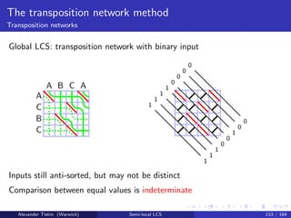
- 47. Matrix distance multiplication Bruhat order Bruhat order Permutation A is lower (“more sorted”) than permutation B in the Bruhat order (A B), if B A by successive pairwise sorting (equivalently, A B by anti-sorting) of arbitrary pairs Permutation matrices: P Q, if Q P by successive 2 × 2 submatrix sorting: ( 0 1 1 0 ) → ( 1 0 0 1 ) Alexander Tiskin (Warwick) Semi-local LCS 28 / 164
- 48. Matrix distance multiplication Bruhat order Bruhat order Permutation A is lower (“more sorted”) than permutation B in the Bruhat order (A B), if B A by successive pairwise sorting (equivalently, A B by anti-sorting) of arbitrary pairs Permutation matrices: P Q, if Q P by successive 2 × 2 submatrix sorting: ( 0 1 1 0 ) → ( 1 0 0 1 ) Plays an important role in group theory and algebraic geometry (inclusion order of Schubert varieties) Describes pivoting order in Gaussian elimination (matrix Bruhat decomposition) Alexander Tiskin (Warwick) Semi-local LCS 28 / 164
- 49. Matrix distance multiplication Bruhat order Bruhat comparability: running time O(n2) [Ehresmann: 1934; Proctor: 1982; Grigoriev: 1982] O(n log n) [T: 2013] O n log n log log n [Gawrychowski: NEW] Alexander Tiskin (Warwick) Semi-local LCS 29 / 164
- 50. Matrix distance multiplication Bruhat order Ehresmann’s criterion (dot criterion, related to tableau criterion) P Q iff PΣ ≤ QΣ elementwise 1 0 0 0 0 1 0 1 0 Σ = 0 1 2 3 0 0 1 2 0 0 1 1 0 0 0 0 ≤ 0 1 2 3 0 1 2 2 0 0 1 1 0 0 0 0 = 0 0 1 1 0 0 0 1 0 Σ 1 0 0 0 0 1 0 1 0 Σ = 0 1 2 3 0 0 1 2 0 0 1 1 0 0 0 0 ≤ 0 1 2 3 0 1 1 2 0 0 0 1 0 0 0 0 = 0 1 0 1 0 0 0 0 1 Σ Time O(n2) Alexander Tiskin (Warwick) Semi-local LCS 30 / 164
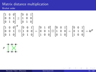
- 51. Matrix distance multiplication Bruhat order Seaweed criterion P Q iff PR Q = IdR , where PR = counterclockwise rotation of P Intuition: permutations represented by seaweed braids P Q, iff no pair of seaweeds is crossed in P, while the “corresponding” pair is uncrossed in Q equivalently, no pair is uncrossed in PR, while the “corresponding” pair is uncrossed in Q equivalently, PR Q = IdR Time O(n log n) by seaweed matrix multiplication Alexander Tiskin (Warwick) Semi-local LCS 31 / 164
- 52. Matrix distance multiplication Bruhat order 1 0 0 0 0 1 0 1 0 0 0 1 1 0 0 0 1 0 1 0 0 0 0 1 0 1 0 R 0 0 1 1 0 0 0 1 0 = 0 1 0 0 0 1 1 0 0 0 0 1 1 0 0 0 1 0 = 0 0 1 0 1 0 1 0 0 = IdR P Alexander Tiskin (Warwick) Semi-local LCS 32 / 164
- 53. Matrix distance multiplication Bruhat order 1 0 0 0 0 1 0 1 0 0 0 1 1 0 0 0 1 0 1 0 0 0 0 1 0 1 0 R 0 0 1 1 0 0 0 1 0 = 0 1 0 0 0 1 1 0 0 0 0 1 1 0 0 0 1 0 = 0 0 1 0 1 0 1 0 0 = IdR P Q Alexander Tiskin (Warwick) Semi-local LCS 32 / 164
- 54. Matrix distance multiplication Bruhat order 1 0 0 0 0 1 0 1 0 0 0 1 1 0 0 0 1 0 1 0 0 0 0 1 0 1 0 R 0 0 1 1 0 0 0 1 0 = 0 1 0 0 0 1 1 0 0 0 0 1 1 0 0 0 1 0 = 0 0 1 0 1 0 1 0 0 = IdR P Q PR Q = Alexander Tiskin (Warwick) Semi-local LCS 32 / 164
- 55. Matrix distance multiplication Bruhat order 1 0 0 0 0 1 0 1 0 0 0 1 1 0 0 0 1 0 1 0 0 0 0 1 0 1 0 R 0 0 1 1 0 0 0 1 0 = 0 1 0 0 0 1 1 0 0 0 0 1 1 0 0 0 1 0 = 0 0 1 0 1 0 1 0 0 = IdR P Q PR Q = IdR Alexander Tiskin (Warwick) Semi-local LCS 32 / 164
- 56. Matrix distance multiplication Bruhat order 1 0 0 0 0 1 0 1 0 0 1 0 1 0 0 0 0 1 1 0 0 0 0 1 0 1 0 R 0 1 0 1 0 0 0 0 1 = 0 1 0 0 0 1 1 0 0 0 1 0 1 0 0 0 0 1 = 0 1 0 0 0 1 1 0 0 = IdR P Alexander Tiskin (Warwick) Semi-local LCS 33 / 164
- 57. Matrix distance multiplication Bruhat order 1 0 0 0 0 1 0 1 0 0 1 0 1 0 0 0 0 1 1 0 0 0 0 1 0 1 0 R 0 1 0 1 0 0 0 0 1 = 0 1 0 0 0 1 1 0 0 0 1 0 1 0 0 0 0 1 = 0 1 0 0 0 1 1 0 0 = IdR P Q Alexander Tiskin (Warwick) Semi-local LCS 33 / 164
- 58. Matrix distance multiplication Bruhat order 1 0 0 0 0 1 0 1 0 0 1 0 1 0 0 0 0 1 1 0 0 0 0 1 0 1 0 R 0 1 0 1 0 0 0 0 1 = 0 1 0 0 0 1 1 0 0 0 1 0 1 0 0 0 0 1 = 0 1 0 0 0 1 1 0 0 = IdR P Q PR Q = Alexander Tiskin (Warwick) Semi-local LCS 33 / 164
- 59. Matrix distance multiplication Bruhat order 1 0 0 0 0 1 0 1 0 0 1 0 1 0 0 0 0 1 1 0 0 0 0 1 0 1 0 R 0 1 0 1 0 0 0 0 1 = 0 1 0 0 0 1 1 0 0 0 1 0 1 0 0 0 0 1 = 0 1 0 0 0 1 1 0 0 = IdR P Q PR Q = = IdR Alexander Tiskin (Warwick) Semi-local LCS 33 / 164
- 60. Matrix distance multiplication Bruhat order Alternative solution: clever implementation of Ehresmann’s criterion [Gawrychowski: 2013] The online partial sums problem: maintain array X[1 : n], subject to update(k, ∆): X[k] ← X[k] + ∆ prefixsum(k): return 1≤i≤k X[i] Query time: Θ(log n) in semigroup or group model Θ log n log log n in RAM model on integers [Pˇatra¸scu, Demaine: 2004] Gives Bruhat comparability in time O n log n log log n in RAM model Open problem: seaweed multiplication in time O n log n log log n ? Alexander Tiskin (Warwick) Semi-local LCS 34 / 164
- 61. 1 Introduction 2 Matrix distance multiplication 3 Semi-local string comparison 4 The seaweed method 5 Periodic string comparison 6 Sparse string comparison 7 Compressed string comparison 8 Parallel string comparison 9 The transposition network method 10 Beyond semi-locality Alexander Tiskin (Warwick) Semi-local LCS 35 / 164
- 62. Semi-local string comparison Semi-local LCS and edit distance Consider strings (= sequences) over an alphabet of size σ Contiguous substrings vs not necessarily contiguous subsequences Special cases of substring: prefix, suffix Notation: strings a, b of length m, n respectively Assume where necessary: m ≤ n; m, n reasonably close Alexander Tiskin (Warwick) Semi-local LCS 36 / 164
- 63. Semi-local string comparison Semi-local LCS and edit distance Consider strings (= sequences) over an alphabet of size σ Contiguous substrings vs not necessarily contiguous subsequences Special cases of substring: prefix, suffix Notation: strings a, b of length m, n respectively Assume where necessary: m ≤ n; m, n reasonably close The longest common subsequence (LCS) score: length of longest string that is a subsequence of both a and b equivalently, alignment score, where score(match) = 1 and score(mismatch) = 0 In biological terms, “loss-free alignment” (unlike efficient but “lossy” BLAST) Alexander Tiskin (Warwick) Semi-local LCS 36 / 164
- 64. Semi-local string comparison Semi-local LCS and edit distance The LCS problem Give the LCS score for a vs b Alexander Tiskin (Warwick) Semi-local LCS 37 / 164
- 65. Semi-local string comparison Semi-local LCS and edit distance The LCS problem Give the LCS score for a vs b LCS: running time O(mn) [Wagner, Fischer: 1974] O mn log2 n σ = O(1) [Masek, Paterson: 1980] [Crochemore+: 2003] O mn(log log n)2 log2 n [Paterson, Danˇc´ık: 1994] [Bille, Farach-Colton: 2008] Running time varies depending on the RAM model version We assume word-RAM with word size log n (where it matters) Alexander Tiskin (Warwick) Semi-local LCS 37 / 164
- 66. Semi-local string comparison Semi-local LCS and edit distance LCS computation by dynamic programming lcs(a, ∅) = 0 lcs(∅, b) = 0 lcs(aα, bβ) = max(lcs(aα, b), lcs(a, bβ)) if α = β lcs(a, b) + 1 if α = β Alexander Tiskin (Warwick) Semi-local LCS 38 / 164
- 67. Semi-local string comparison Semi-local LCS and edit distance LCS computation by dynamic programming lcs(a, ∅) = 0 lcs(∅, b) = 0 lcs(aα, bβ) = max(lcs(aα, b), lcs(a, bβ)) if α = β lcs(a, b) + 1 if α = β ∗ D E F I N E ∗ 0 0 0 0 0 0 0 D 0 E 0 S 0 I 0 G 0 N 0 Alexander Tiskin (Warwick) Semi-local LCS 38 / 164
- 68. Semi-local string comparison Semi-local LCS and edit distance LCS computation by dynamic programming lcs(a, ∅) = 0 lcs(∅, b) = 0 lcs(aα, bβ) = max(lcs(aα, b), lcs(a, bβ)) if α = β lcs(a, b) + 1 if α = β ∗ D E F I N E ∗ 0 0 0 0 0 0 0 D 0 1 E 0 S 0 I 0 G 0 N 0 Alexander Tiskin (Warwick) Semi-local LCS 38 / 164
- 69. Semi-local string comparison Semi-local LCS and edit distance LCS computation by dynamic programming lcs(a, ∅) = 0 lcs(∅, b) = 0 lcs(aα, bβ) = max(lcs(aα, b), lcs(a, bβ)) if α = β lcs(a, b) + 1 if α = β ∗ D E F I N E ∗ 0 0 0 0 0 0 0 D 0 1 1 E 0 S 0 I 0 G 0 N 0 Alexander Tiskin (Warwick) Semi-local LCS 38 / 164
- 70. Semi-local string comparison Semi-local LCS and edit distance LCS computation by dynamic programming lcs(a, ∅) = 0 lcs(∅, b) = 0 lcs(aα, bβ) = max(lcs(aα, b), lcs(a, bβ)) if α = β lcs(a, b) + 1 if α = β ∗ D E F I N E ∗ 0 0 0 0 0 0 0 D 0 1 1 1 1 1 1 E 0 S 0 I 0 G 0 N 0 Alexander Tiskin (Warwick) Semi-local LCS 38 / 164
- 71. Semi-local string comparison Semi-local LCS and edit distance LCS computation by dynamic programming lcs(a, ∅) = 0 lcs(∅, b) = 0 lcs(aα, bβ) = max(lcs(aα, b), lcs(a, bβ)) if α = β lcs(a, b) + 1 if α = β ∗ D E F I N E ∗ 0 0 0 0 0 0 0 D 0 1 1 1 1 1 1 E 0 1 S 0 I 0 G 0 N 0 Alexander Tiskin (Warwick) Semi-local LCS 38 / 164
- 72. Semi-local string comparison Semi-local LCS and edit distance LCS computation by dynamic programming lcs(a, ∅) = 0 lcs(∅, b) = 0 lcs(aα, bβ) = max(lcs(aα, b), lcs(a, bβ)) if α = β lcs(a, b) + 1 if α = β ∗ D E F I N E ∗ 0 0 0 0 0 0 0 D 0 1 1 1 1 1 1 E 0 1 2 S 0 I 0 G 0 N 0 Alexander Tiskin (Warwick) Semi-local LCS 38 / 164
- 73. Semi-local string comparison Semi-local LCS and edit distance LCS computation by dynamic programming lcs(a, ∅) = 0 lcs(∅, b) = 0 lcs(aα, bβ) = max(lcs(aα, b), lcs(a, bβ)) if α = β lcs(a, b) + 1 if α = β ∗ D E F I N E ∗ 0 0 0 0 0 0 0 D 0 1 1 1 1 1 1 E 0 1 2 2 2 2 2 S 0 I 0 G 0 N 0 Alexander Tiskin (Warwick) Semi-local LCS 38 / 164
- 74. Semi-local string comparison Semi-local LCS and edit distance LCS computation by dynamic programming lcs(a, ∅) = 0 lcs(∅, b) = 0 lcs(aα, bβ) = max(lcs(aα, b), lcs(a, bβ)) if α = β lcs(a, b) + 1 if α = β ∗ D E F I N E ∗ 0 0 0 0 0 0 0 D 0 1 1 1 1 1 1 E 0 1 2 2 2 2 2 S 0 1 2 2 2 2 2 I 0 G 0 N 0 Alexander Tiskin (Warwick) Semi-local LCS 38 / 164
- 75. Semi-local string comparison Semi-local LCS and edit distance LCS computation by dynamic programming lcs(a, ∅) = 0 lcs(∅, b) = 0 lcs(aα, bβ) = max(lcs(aα, b), lcs(a, bβ)) if α = β lcs(a, b) + 1 if α = β ∗ D E F I N E ∗ 0 0 0 0 0 0 0 D 0 1 1 1 1 1 1 E 0 1 2 2 2 2 2 S 0 1 2 2 2 2 2 I 0 1 2 2 3 3 3 G 0 N 0 Alexander Tiskin (Warwick) Semi-local LCS 38 / 164
- 76. Semi-local string comparison Semi-local LCS and edit distance LCS computation by dynamic programming lcs(a, ∅) = 0 lcs(∅, b) = 0 lcs(aα, bβ) = max(lcs(aα, b), lcs(a, bβ)) if α = β lcs(a, b) + 1 if α = β ∗ D E F I N E ∗ 0 0 0 0 0 0 0 D 0 1 1 1 1 1 1 E 0 1 2 2 2 2 2 S 0 1 2 2 2 2 2 I 0 1 2 2 3 3 3 G 0 1 2 2 3 3 3 N 0 1 2 2 3 4 4 Alexander Tiskin (Warwick) Semi-local LCS 38 / 164
- 77. Semi-local string comparison Semi-local LCS and edit distance LCS computation by dynamic programming lcs(a, ∅) = 0 lcs(∅, b) = 0 lcs(aα, bβ) = max(lcs(aα, b), lcs(a, bβ)) if α = β lcs(a, b) + 1 if α = β ∗ D E F I N E ∗ 0 0 0 0 0 0 0 D 0 1 1 1 1 1 1 E 0 1 2 2 2 2 2 S 0 1 2 2 2 2 2 I 0 1 2 2 3 3 3 G 0 1 2 2 3 3 3 N 0 1 2 2 3 4 4 lcs(“DEFINE”, “DESIGN”) = 4 Alexander Tiskin (Warwick) Semi-local LCS 38 / 164
- 78. Semi-local string comparison Semi-local LCS and edit distance LCS computation by dynamic programming lcs(a, ∅) = 0 lcs(∅, b) = 0 lcs(aα, bβ) = max(lcs(aα, b), lcs(a, bβ)) if α = β lcs(a, b) + 1 if α = β ∗ D E F I N E ∗ 0 0 0 0 0 0 0 D 0 1 1 1 1 1 1 E 0 1 2 2 2 2 2 S 0 1 2 2 2 2 2 I 0 1 2 2 3 3 3 G 0 1 2 2 3 3 3 N 0 1 2 2 3 4 4 lcs(“DEFINE”, “DESIGN”) = 4 LCS(a, b) can be traced back through the dynamic programming table at no extra asymptotic time cost Alexander Tiskin (Warwick) Semi-local LCS 38 / 164
- 79. Semi-local string comparison Semi-local LCS and edit distance LCS on the alignment graph: directed grid of match and mismatch cells B A A B C B C A B A A B C A B C A B A C A blue = 0 red = 1 score(“BAABCBCA”, “BAABCABCABACA”) = len(“BAABCBCA”) = 8 LCS = highest-score path from top-left to bottom-right Alexander Tiskin (Warwick) Semi-local LCS 39 / 164
- 80. Semi-local string comparison Semi-local LCS and edit distance LCS: dynamic programming [WF: 1974] Sweep cells in any -compatible order Cell update: time O(1) Overall time O(mn) Alexander Tiskin (Warwick) Semi-local LCS 40 / 164
- 81. Semi-local string comparison Semi-local LCS and edit distance LCS: micro-block dynamic programming [MP: 1980; BF: 2008] Sweep cells in micro-blocks, in any -compatible order Micro-block size: t = O(log n) when σ = O(1) t = O log n log log n otherwise Micro-block interface: O(t) characters, each O(log σ) bits, can be reduced to O(log t) bits O(t) small integers, each O(1) bits Micro-block update: time O(1), by precomputing all possible interfaces Overall time O mn log2 n when σ = O(1), O mn(log log n)2 log2 n otherwise Alexander Tiskin (Warwick) Semi-local LCS 41 / 164
- 82. Semi-local string comparison Semi-local LCS and edit distance ‘Begin at the beginning,’ the King said gravely, ‘and go on till you come to the end: then stop.’ L. Carroll, Alice in Wonderland Alexander Tiskin (Warwick) Semi-local LCS 42 / 164
- 83. Semi-local string comparison Semi-local LCS and edit distance ‘Begin at the beginning,’ the King said gravely, ‘and go on till you come to the end: then stop.’ L. Carroll, Alice in Wonderland Dynamic programming: begins at empty strings, proceeds by appending characters, then stops What about: prepending/deleting characters (dynamic LCS) concatenating strings (LCS on compressed strings; parallel LCS) taking substrings (= local alignment) Alexander Tiskin (Warwick) Semi-local LCS 42 / 164
- 84. Semi-local string comparison Semi-local LCS and edit distance Dynamic programming from both ends: better by ×2, but still not good enough Is dynamic programming strictly necessary to solve sequence alignment problems? Eppstein+, Efficient algorithms for sequence analysis, 1991 Alexander Tiskin (Warwick) Semi-local LCS 43 / 164
- 85. Semi-local string comparison Semi-local LCS and edit distance The semi-local LCS problem Give the (implicit) matrix of O (m + n)2 LCS scores: string-substring LCS: string a vs every substring of b prefix-suffix LCS: every prefix of a vs every suffix of b suffix-prefix LCS: every suffix of a vs every prefix of b substring-string LCS: every substring of a vs string b Alexander Tiskin (Warwick) Semi-local LCS 44 / 164
- 86. Semi-local string comparison Semi-local LCS and edit distance The semi-local LCS problem Give the (implicit) matrix of O (m + n)2 LCS scores: string-substring LCS: string a vs every substring of b prefix-suffix LCS: every prefix of a vs every suffix of b suffix-prefix LCS: every suffix of a vs every prefix of b substring-string LCS: every substring of a vs string b Alexander Tiskin (Warwick) Semi-local LCS 44 / 164
- 87. Semi-local string comparison Semi-local LCS and edit distance Semi-local LCS on the alignment graph B A A B C B C A B A A B C A B C A B A C AC A B C A B A blue = 0 red = 1 score(“BAABCBCA”, “CABCABA”) = len(“ABCBA”) = 5 String-substring LCS: all highest-score top-to-bottom paths Semi-local LCS: all highest-score boundary-to-boundary paths Alexander Tiskin (Warwick) Semi-local LCS 45 / 164
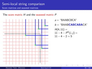
- 88. Semi-local string comparison Score matrices and seaweed matrices The score matrix H 0 1 2 3 4 5 6 6 7 8 8 8 8 8 -1 0 1 2 3 4 5 5 6 7 7 7 7 7 -2 -1 0 1 2 3 4 4 5 6 6 6 6 7 -3 -2 -1 0 1 2 3 3 4 5 5 6 6 7 -4 -3 -2 -1 0 1 2 2 3 4 4 5 5 6 -5 -4 -3 -2 -1 0 1 2 3 4 4 5 5 6 -6 -5 -4 -3 -2 -1 0 1 2 3 3 4 4 5 -7 -6 -5 -4 -3 -2 -1 0 1 2 2 3 3 4 -8 -7 -6 -5 -4 -3 -2 -1 0 1 2 3 3 4 -9 -8 -7 -6 -5 -4 -3 -2 -1 0 1 2 3 4 -10 -9 -8 -7 -6 -5 -4 -3 -2 -1 0 1 2 3 -11 -10 -9 -8 -7 -6 -5 -4 -3 -2 -1 0 1 2 -12 -11 -10 -9 -8 -7 -6 -5 -4 -3 -2 -1 0 1 -13 -12 -11 -10 -9 -8 -7 -6 -5 -4 -3 -2 -1 0 5 a = “BAABCBCA” b = “BAABCABCABACA” H(i, j) = score(a, b i : j ) H(4, 11) = 5 H(i, j) = j − i if i > j Alexander Tiskin (Warwick) Semi-local LCS 46 / 164
- 89. Semi-local string comparison Score matrices and seaweed matrices Semi-local LCS: output representation and running time size query time O(n2) O(1) trivial O(m1/2n) O(log n) string-substring [Alves+: 2003] O(n) O(n) string-substring [Alves+: 2005] O(n log n) O(log2 n) [T: 2006] . . . or any 2D orthogonal range counting data structure running time O(mn2) naive O(mn) string-substring [Schmidt: 1998; Alves+: 2005] O(mn) [T: 2006] O mn log0.5 n [T: 2006] O mn(log log n)2 log2 n [T: 2007] Alexander Tiskin (Warwick) Semi-local LCS 47 / 164
- 90. Semi-local string comparison Score matrices and seaweed matrices The score matrix H and the seaweed matrix P H(i, j): the number of matched characters for a vs substring b i : j j − i − H(i, j): the number of unmatched characters Properties of matrix j − i − H(i, j): simple unit-Monge therefore, = PΣ, where P = −H is a permutation matrix P is the seaweed matrix, giving an implicit representation of H Range tree for P: memory O(n log n), query time O(log2 n) Alexander Tiskin (Warwick) Semi-local LCS 48 / 164
- 91. Semi-local string comparison Score matrices and seaweed matrices The score matrix H and the seaweed matrix P 0 1 2 3 4 5 6 6 7 8 8 8 8 8 -1 0 1 2 3 4 5 5 6 7 7 7 7 7 -2 -1 0 1 2 3 4 4 5 6 6 6 6 7 -3 -2 -1 0 1 2 3 3 4 5 5 6 6 7 -4 -3 -2 -1 0 1 2 2 3 4 4 5 5 6 -5 -4 -3 -2 -1 0 1 2 3 4 4 5 5 6 -6 -5 -4 -3 -2 -1 0 1 2 3 3 4 4 5 -7 -6 -5 -4 -3 -2 -1 0 1 2 2 3 3 4 -8 -7 -6 -5 -4 -3 -2 -1 0 1 2 3 3 4 -9 -8 -7 -6 -5 -4 -3 -2 -1 0 1 2 3 4 -10 -9 -8 -7 -6 -5 -4 -3 -2 -1 0 1 2 3 -11 -10 -9 -8 -7 -6 -5 -4 -3 -2 -1 0 1 2 -12 -11 -10 -9 -8 -7 -6 -5 -4 -3 -2 -1 0 1 -13 -12 -11 -10 -9 -8 -7 -6 -5 -4 -3 -2 -1 0 5 a = “BAABCBCA” b = “BAABCABCABACA” H(i, j) = score(a, b i : j ) H(4, 11) = 5 H(i, j) = j − i if i > j Alexander Tiskin (Warwick) Semi-local LCS 49 / 164
- 92. Semi-local string comparison Score matrices and seaweed matrices The score matrix H and the seaweed matrix P 0 1 2 3 4 5 6 6 7 8 8 8 8 8 -1 0 1 2 3 4 5 5 6 7 7 7 7 7 -2 -1 0 1 2 3 4 4 5 6 6 6 6 7 -3 -2 -1 0 1 2 3 3 4 5 5 6 6 7 -4 -3 -2 -1 0 1 2 2 3 4 4 5 5 6 -5 -4 -3 -2 -1 0 1 2 3 4 4 5 5 6 -6 -5 -4 -3 -2 -1 0 1 2 3 3 4 4 5 -7 -6 -5 -4 -3 -2 -1 0 1 2 2 3 3 4 -8 -7 -6 -5 -4 -3 -2 -1 0 1 2 3 3 4 -9 -8 -7 -6 -5 -4 -3 -2 -1 0 1 2 3 4 -10 -9 -8 -7 -6 -5 -4 -3 -2 -1 0 1 2 3 -11 -10 -9 -8 -7 -6 -5 -4 -3 -2 -1 0 1 2 -12 -11 -10 -9 -8 -7 -6 -5 -4 -3 -2 -1 0 1 -13 -12 -11 -10 -9 -8 -7 -6 -5 -4 -3 -2 -1 0 5 a = “BAABCBCA” b = “BAABCABCABACA” H(i, j) = score(a, b i : j ) H(4, 11) = 5 H(i, j) = j − i if i > j blue: difference in H is 0 red: difference in H is 1 Alexander Tiskin (Warwick) Semi-local LCS 49 / 164
- 93. Semi-local string comparison Score matrices and seaweed matrices The score matrix H and the seaweed matrix P 0 1 2 3 4 5 6 6 7 8 8 8 8 8 -1 0 1 2 3 4 5 5 6 7 7 7 7 7 -2 -1 0 1 2 3 4 4 5 6 6 6 6 7 -3 -2 -1 0 1 2 3 3 4 5 5 6 6 7 -4 -3 -2 -1 0 1 2 2 3 4 4 5 5 6 -5 -4 -3 -2 -1 0 1 2 3 4 4 5 5 6 -6 -5 -4 -3 -2 -1 0 1 2 3 3 4 4 5 -7 -6 -5 -4 -3 -2 -1 0 1 2 2 3 3 4 -8 -7 -6 -5 -4 -3 -2 -1 0 1 2 3 3 4 -9 -8 -7 -6 -5 -4 -3 -2 -1 0 1 2 3 4 -10 -9 -8 -7 -6 -5 -4 -3 -2 -1 0 1 2 3 -11 -10 -9 -8 -7 -6 -5 -4 -3 -2 -1 0 1 2 -12 -11 -10 -9 -8 -7 -6 -5 -4 -3 -2 -1 0 1 -13 -12 -11 -10 -9 -8 -7 -6 -5 -4 -3 -2 -1 0 5 a = “BAABCBCA” b = “BAABCABCABACA” H(i, j) = score(a, b i : j ) H(4, 11) = 5 H(i, j) = j − i if i > j blue: difference in H is 0 red: difference in H is 1 green: P(i, j) = 1 H(i, j) = j − i − PΣ(i, j) Alexander Tiskin (Warwick) Semi-local LCS 49 / 164
- 94. Semi-local string comparison Score matrices and seaweed matrices The score matrix H and the seaweed matrix P a = “BAABCBCA” b = “BAABCABCABACA” H(4, 11) = 11 − 4 − PΣ(i, j) = 11 − 4 − 2 = 5 Alexander Tiskin (Warwick) Semi-local LCS 50 / 164
- 95. Semi-local string comparison Score matrices and seaweed matrices The (combed) seaweed braid in the alignment graph B A A B C B C A B A A B C A B C A B A C AC A B C A B A a = “BAABCBCA” b = “BAABCABCABACA” H(4, 11) = 11 − 4 − PΣ(i, j) = 11 − 4 − 2 = 5 P(i, j) = 1 corresponds to seaweed top i bottom j Alexander Tiskin (Warwick) Semi-local LCS 51 / 164
- 96. Semi-local string comparison Score matrices and seaweed matrices The (combed) seaweed braid in the alignment graph B A A B C B C A B A A B C A B C A B A C AC A B C A B A a = “BAABCBCA” b = “BAABCABCABACA” H(4, 11) = 11 − 4 − PΣ(i, j) = 11 − 4 − 2 = 5 P(i, j) = 1 corresponds to seaweed top i bottom j Also define seaweeds top right, left right, left bottom Represent implicitly semi-local LCS for each prefix of a vs b Alexander Tiskin (Warwick) Semi-local LCS 51 / 164
- 97. Semi-local string comparison Score matrices and seaweed matrices Seaweed braid: a highly symmetric object (element of H0(Sn)) Can be built by assembling subbraids: divide-and-conquer Flexible approach to local alignment, compressed approximate matching, parallel computation. . . Alexander Tiskin (Warwick) Semi-local LCS 52 / 164
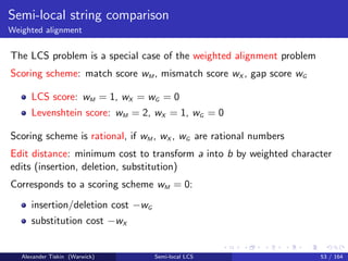
- 98. Semi-local string comparison Weighted alignment The LCS problem is a special case of the weighted alignment problem Scoring scheme: match score wM , mismatch score wX , gap score wG LCS score: wM = 1, wX = wG = 0 Levenshtein score: wM = 2, wX = 1, wG = 0 Alexander Tiskin (Warwick) Semi-local LCS 53 / 164
- 99. Semi-local string comparison Weighted alignment The LCS problem is a special case of the weighted alignment problem Scoring scheme: match score wM , mismatch score wX , gap score wG LCS score: wM = 1, wX = wG = 0 Levenshtein score: wM = 2, wX = 1, wG = 0 Scoring scheme is rational, if wM , wX , wG are rational numbers Alexander Tiskin (Warwick) Semi-local LCS 53 / 164
- 100. Semi-local string comparison Weighted alignment The LCS problem is a special case of the weighted alignment problem Scoring scheme: match score wM , mismatch score wX , gap score wG LCS score: wM = 1, wX = wG = 0 Levenshtein score: wM = 2, wX = 1, wG = 0 Scoring scheme is rational, if wM , wX , wG are rational numbers Edit distance: minimum cost to transform a into b by weighted character edits (insertion, deletion, substitution) Corresponds to a scoring scheme wM = 0: insertion/deletion cost −wG substitution cost −wX Alexander Tiskin (Warwick) Semi-local LCS 53 / 164
- 101. Semi-local string comparison Weighted alignment Weighted alignment graph for a, b B A A B C B C A B A A B C A B C A B A C AC A B C A B A blue = 0 red (solid) = 2 red (dotted) = 1 Levenshtein(“BAABCBCA”, “CABCABA”) = 11 Alexander Tiskin (Warwick) Semi-local LCS 54 / 164
- 102. Semi-local string comparison Weighted alignment Reduction: ordinary alignment graph for blown-up a, b $B $A $A $B $C $B $C $A $B $A $A $B $C $A $B $C $A $B $A $C $A$C $A$B $C $A$B$A blue = 0 red = 1 or 2 Levenshtein(“BAABCBCA”, “CABCABA”) = lcs(“$B$A$A$B$C$B$C$A”, “$C$A$B$C$A$B$A”) = 11 Alexander Tiskin (Warwick) Semi-local LCS 55 / 164
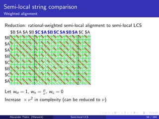
- 103. Semi-local string comparison Weighted alignment Reduction: rational-weighted semi-local alignment to semi-local LCS $B $A $A $B $C $B $C $A $B $A $A $B $C $A $B $C $A $B $A $C $A$C $A$B $C $A$B$A Let wM = 1, wX = µ ν , wG = 0 Increase × ν2 in complexity (can be reduced to ν) Alexander Tiskin (Warwick) Semi-local LCS 56 / 164
- 104. 1 Introduction 2 Matrix distance multiplication 3 Semi-local string comparison 4 The seaweed method 5 Periodic string comparison 6 Sparse string comparison 7 Compressed string comparison 8 Parallel string comparison 9 The transposition network method 10 Beyond semi-locality Alexander Tiskin (Warwick) Semi-local LCS 57 / 164
- 105. The seaweed method Seaweed combing B A A B C B C A B A A B C A B C A B A C A Alexander Tiskin (Warwick) Semi-local LCS 58 / 164
- 106. The seaweed method Seaweed combing B A A B C B C A B A A B C A B C A B A C A Alexander Tiskin (Warwick) Semi-local LCS 59 / 164
- 107. The seaweed method Seaweed combing B A A B C B C A B A A B C A B C A B A C A Alexander Tiskin (Warwick) Semi-local LCS 59 / 164
- 108. The seaweed method Seaweed combing B A A B C B C A B A A B C A B C A B A C A Alexander Tiskin (Warwick) Semi-local LCS 59 / 164
- 109. The seaweed method Seaweed combing B A A B C B C A B A A B C A B C A B A C A Alexander Tiskin (Warwick) Semi-local LCS 59 / 164
- 110. The seaweed method Seaweed combing B A A B C B C A B A A B C A B C A B A C A Alexander Tiskin (Warwick) Semi-local LCS 59 / 164
- 111. The seaweed method Seaweed combing B A A B C B C A B A A B C A B C A B A C A Alexander Tiskin (Warwick) Semi-local LCS 59 / 164
- 112. The seaweed method Seaweed combing B A A B C B C A B A A B C A B C A B A C A Alexander Tiskin (Warwick) Semi-local LCS 59 / 164
- 113. The seaweed method Seaweed combing B A A B C B C A B A A B C A B C A B A C A Alexander Tiskin (Warwick) Semi-local LCS 59 / 164
- 114. The seaweed method Seaweed combing B A A B C B C A B A A B C A B C A B A C A Alexander Tiskin (Warwick) Semi-local LCS 59 / 164
- 115. The seaweed method Seaweed combing B A A B C B C A B A A B C A B C A B A C A Alexander Tiskin (Warwick) Semi-local LCS 59 / 164
- 116. The seaweed method Seaweed combing B A A B C B C A B A A B C A B C A B A C A Alexander Tiskin (Warwick) Semi-local LCS 59 / 164
- 117. The seaweed method Seaweed combing B A A B C B C A B A A B C A B C A B A C A Alexander Tiskin (Warwick) Semi-local LCS 59 / 164
- 118. The seaweed method Seaweed combing B A A B C B C A B A A B C A B C A B A C A Alexander Tiskin (Warwick) Semi-local LCS 59 / 164
- 119. The seaweed method Seaweed combing B A A B C B C A B A A B C A B C A B A C A Alexander Tiskin (Warwick) Semi-local LCS 59 / 164
- 120. The seaweed method Seaweed combing B A A B C B C A B A A B C A B C A B A C A Alexander Tiskin (Warwick) Semi-local LCS 59 / 164
- 121. The seaweed method Seaweed combing B A A B C B C A B A A B C A B C A B A C A Alexander Tiskin (Warwick) Semi-local LCS 59 / 164
- 122. The seaweed method Seaweed combing B A A B C B C A B A A B C A B C A B A C A Alexander Tiskin (Warwick) Semi-local LCS 59 / 164
- 123. The seaweed method Seaweed combing B A A B C B C A B A A B C A B C A B A C A Alexander Tiskin (Warwick) Semi-local LCS 59 / 164
- 124. The seaweed method Seaweed combing B A A B C B C A B A A B C A B C A B A C A Alexander Tiskin (Warwick) Semi-local LCS 59 / 164
- 125. The seaweed method Seaweed combing B A A B C B C A B A A B C A B C A B A C A Alexander Tiskin (Warwick) Semi-local LCS 59 / 164
- 126. The seaweed method Seaweed combing B A A B C B C A B A A B C A B C A B A C A Alexander Tiskin (Warwick) Semi-local LCS 59 / 164
- 127. The seaweed method Seaweed combing B A A B C B C A B A A B C A B C A B A C A Alexander Tiskin (Warwick) Semi-local LCS 59 / 164
- 128. The seaweed method Seaweed combing B A A B C B C A B A A B C A B C A B A C A Alexander Tiskin (Warwick) Semi-local LCS 59 / 164
- 129. The seaweed method Seaweed combing B A A B C B C A B A A B C A B C A B A C A Alexander Tiskin (Warwick) Semi-local LCS 59 / 164
- 130. The seaweed method Seaweed combing B A A B C B C A B A A B C A B C A B A C A Alexander Tiskin (Warwick) Semi-local LCS 59 / 164
- 131. The seaweed method Seaweed combing B A A B C B C A B A A B C A B C A B A C A Alexander Tiskin (Warwick) Semi-local LCS 59 / 164
- 132. The seaweed method Seaweed combing B A A B C B C A B A A B C A B C A B A C A Alexander Tiskin (Warwick) Semi-local LCS 59 / 164
- 133. The seaweed method Seaweed combing B A A B C B C A B A A B C A B C A B A C A Alexander Tiskin (Warwick) Semi-local LCS 59 / 164
- 134. The seaweed method Seaweed combing B A A B C B C A B A A B C A B C A B A C A Alexander Tiskin (Warwick) Semi-local LCS 59 / 164
- 135. The seaweed method Seaweed combing B A A B C B C A B A A B C A B C A B A C A Alexander Tiskin (Warwick) Semi-local LCS 59 / 164
- 136. The seaweed method Seaweed combing B A A B C B C A B A A B C A B C A B A C A Alexander Tiskin (Warwick) Semi-local LCS 59 / 164
- 137. The seaweed method Seaweed combing B A A B C B C A B A A B C A B C A B A C A Alexander Tiskin (Warwick) Semi-local LCS 59 / 164
- 138. The seaweed method Seaweed combing B A A B C B C A B A A B C A B C A B A C A Alexander Tiskin (Warwick) Semi-local LCS 59 / 164
- 139. The seaweed method Seaweed combing B A A B C B C A B A A B C A B C A B A C A Alexander Tiskin (Warwick) Semi-local LCS 59 / 164
- 140. The seaweed method Seaweed combing B A A B C B C A B A A B C A B C A B A C A Alexander Tiskin (Warwick) Semi-local LCS 59 / 164
- 141. The seaweed method Seaweed combing B A A B C B C A B A A B C A B C A B A C A Alexander Tiskin (Warwick) Semi-local LCS 59 / 164
- 142. The seaweed method Seaweed combing B A A B C B C A B A A B C A B C A B A C A Alexander Tiskin (Warwick) Semi-local LCS 59 / 164
- 143. The seaweed method Seaweed combing B A A B C B C A B A A B C A B C A B A C A Alexander Tiskin (Warwick) Semi-local LCS 60 / 164
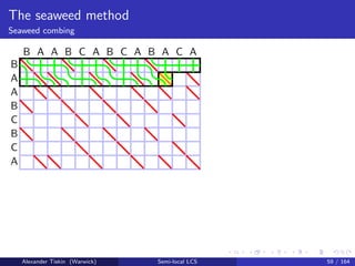
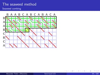
- 144. The seaweed method Seaweed combing Semi-local LCS: seaweed combing [T: 2006] Initialise uncombed seaweed braid: mismatch cell = crossing Sweep cells in any -compatible order match cell: skip (keep uncrossed) mismatch cell: comb (uncross) iff the same seaweed pair already crossed before Cell update: time O(1) Overall time O(mn) Correctness: by seaweed monoid relations Alexander Tiskin (Warwick) Semi-local LCS 61 / 164
- 145. The seaweed method Micro-block seaweed combing B A A B C B C A B A A B C A B C A B A C A Alexander Tiskin (Warwick) Semi-local LCS 62 / 164
- 146. The seaweed method Micro-block seaweed combing B A A B C B C A B A A B C A B C A B A C A Alexander Tiskin (Warwick) Semi-local LCS 63 / 164
- 147. The seaweed method Micro-block seaweed combing B A A B C B C A B A A B C A B C A B A C A Alexander Tiskin (Warwick) Semi-local LCS 63 / 164
- 148. The seaweed method Micro-block seaweed combing B A A B C B C A B A A B C A B C A B A C A Alexander Tiskin (Warwick) Semi-local LCS 63 / 164
- 149. The seaweed method Micro-block seaweed combing B A A B C B C A B A A B C A B C A B A C A Alexander Tiskin (Warwick) Semi-local LCS 63 / 164
- 150. The seaweed method Micro-block seaweed combing B A A B C B C A B A A B C A B C A B A C A Alexander Tiskin (Warwick) Semi-local LCS 63 / 164
- 151. The seaweed method Micro-block seaweed combing B A A B C B C A B A A B C A B C A B A C A Alexander Tiskin (Warwick) Semi-local LCS 63 / 164
- 152. The seaweed method Micro-block seaweed combing B A A B C B C A B A A B C A B C A B A C A Alexander Tiskin (Warwick) Semi-local LCS 63 / 164
- 153. The seaweed method Micro-block seaweed combing B A A B C B C A B A A B C A B C A B A C A Alexander Tiskin (Warwick) Semi-local LCS 63 / 164
- 154. The seaweed method Micro-block seaweed combing B A A B C B C A B A A B C A B C A B A C A Alexander Tiskin (Warwick) Semi-local LCS 63 / 164
- 155. The seaweed method Micro-block seaweed combing B A A B C B C A B A A B C A B C A B A C A Alexander Tiskin (Warwick) Semi-local LCS 63 / 164
- 156. The seaweed method Micro-block seaweed combing B A A B C B C A B A A B C A B C A B A C A Alexander Tiskin (Warwick) Semi-local LCS 63 / 164
- 157. The seaweed method Micro-block seaweed combing B A A B C B C A B A A B C A B C A B A C A Alexander Tiskin (Warwick) Semi-local LCS 63 / 164
- 158. The seaweed method Micro-block seaweed combing B A A B C B C A B A A B C A B C A B A C A Alexander Tiskin (Warwick) Semi-local LCS 63 / 164
- 159. The seaweed method Micro-block seaweed combing B A A B C B C A B A A B C A B C A B A C A Alexander Tiskin (Warwick) Semi-local LCS 64 / 164
- 160. The seaweed method Micro-block seaweed combing Semi-local LCS: micro-block seaweed combing [T: 2007] Initialise uncombed seaweed braid: mismatch cell = crossing Sweep cells in micro-blocks, in any -compatible order Micro-block size: t = O log n log log n Micro-block interface: O(t) characters, each O(log σ) bits, can be reduced to O(log t) bits O(t) integers, each O(log n) bits, can be reduced to O(log t) bits Micro-block update: time O(1), by precomputing all possible interfaces Overall time O mn(log log n)2 log2 n Alexander Tiskin (Warwick) Semi-local LCS 65 / 164
- 161. The seaweed method Cyclic LCS The cyclic LCS problem Give the maximum LCS score for a vs all cyclic rotations of b Alexander Tiskin (Warwick) Semi-local LCS 66 / 164
- 162. The seaweed method Cyclic LCS The cyclic LCS problem Give the maximum LCS score for a vs all cyclic rotations of b Cyclic LCS: running time O mn2 log n naive O(mn log m) [Maes: 1990] O(mn) [Bunke, B¨uhler: 1993; Landau+: 1998; Schmidt: 1998] O mn(log log n)2 log2 n [T: 2007] Alexander Tiskin (Warwick) Semi-local LCS 66 / 164
- 163. The seaweed method Cyclic LCS Cyclic LCS: the algorithm Micro-block seaweed combing on a vs bb, time O mn(log log n)2 log2 n Make n string-substring LCS queries, time negligible Alexander Tiskin (Warwick) Semi-local LCS 67 / 164
- 164. The seaweed method Longest repeating subsequence The longest repeating subsequence problem Find the longest subsequence of a that is a square (a repetition of two identical strings) Alexander Tiskin (Warwick) Semi-local LCS 68 / 164
- 165. The seaweed method Longest repeating subsequence The longest repeating subsequence problem Find the longest subsequence of a that is a square (a repetition of two identical strings) Longest repeating subsequence: running time O(m3) naive O(m2) [Kosowski: 2004] O m2(log log m)2 log2 m [T: 2007] Alexander Tiskin (Warwick) Semi-local LCS 68 / 164
- 166. The seaweed method Longest repeating subsequence Longest repeating subsequence: the algorithm Micro-block seaweed combing on a vs a, time O m2(log log m)2 log2 m Make m − 1 prefix-suffix LCS queries, time negligible Open question: generalise to longest subsequence that is a cube, etc. Alexander Tiskin (Warwick) Semi-local LCS 69 / 164
- 167. The seaweed method Approximate matching The approximate pattern matching problem Give the substring closest to a by alignment score, starting at each position in b Assume rational scoring scheme Approximate pattern matching: running time O(mn) [Sellers: 1980] O mn log n σ = O(1) via [Masek, Paterson: 1980] O mn(log log n)2 log2 n via [Bille, Farach-Colton: 2008] Alexander Tiskin (Warwick) Semi-local LCS 70 / 164
- 168. The seaweed method Approximate matching Approximate pattern matching: the algorithm Micro-block seaweed combing on a vs b (with blow-up), time O mn(log log n)2 log2 n The implicit semi-local edit score matrix: an anti-Monge matrix approximate pattern matching ∼ row minima Row minima in O(n) element queries [Aggarwal+: 1987] Each query in time O(log2 n) using the range tree representation, combined query time negligible Overall running time O mn(log log n)2 log2 n , same as [Bille, Farach-Colton: 2008] Alexander Tiskin (Warwick) Semi-local LCS 71 / 164
- 169. 1 Introduction 2 Matrix distance multiplication 3 Semi-local string comparison 4 The seaweed method 5 Periodic string comparison 6 Sparse string comparison 7 Compressed string comparison 8 Parallel string comparison 9 The transposition network method 10 Beyond semi-locality Alexander Tiskin (Warwick) Semi-local LCS 72 / 164
- 170. Periodic string comparison Wraparound seaweed combing The periodic string-substring LCS problem Give (implicit) LCS scores for a vs each substring of b = . . . uuu . . . = u±∞ Let u be of length p May assume that every character of a occurs in u (otherwise delete it) Only substrings of b of length ≤ mp (otherwise LCS score = m) Alexander Tiskin (Warwick) Semi-local LCS 73 / 164
- 171. Periodic string comparison Wraparound seaweed combing B A A B C B C A B A A B C A B C A B A C A Alexander Tiskin (Warwick) Semi-local LCS 74 / 164
- 172. Periodic string comparison Wraparound seaweed combing B A A B C B C A B A A B C A B C A B A C A Alexander Tiskin (Warwick) Semi-local LCS 75 / 164
- 173. Periodic string comparison Wraparound seaweed combing B A A B C B C A B A A B C A B C A B A C A Alexander Tiskin (Warwick) Semi-local LCS 75 / 164
- 174. Periodic string comparison Wraparound seaweed combing B A A B C B C A B A A B C A B C A B A C A Alexander Tiskin (Warwick) Semi-local LCS 75 / 164
- 175. Periodic string comparison Wraparound seaweed combing B A A B C B C A B A A B C A B C A B A C A Alexander Tiskin (Warwick) Semi-local LCS 75 / 164
- 176. Periodic string comparison Wraparound seaweed combing B A A B C B C A B A A B C A B C A B A C A Alexander Tiskin (Warwick) Semi-local LCS 75 / 164
- 177. Periodic string comparison Wraparound seaweed combing B A A B C B C A B A A B C A B C A B A C A Alexander Tiskin (Warwick) Semi-local LCS 75 / 164
- 178. Periodic string comparison Wraparound seaweed combing B A A B C B C A B A A B C A B C A B A C A Alexander Tiskin (Warwick) Semi-local LCS 75 / 164
- 179. Periodic string comparison Wraparound seaweed combing B A A B C B C A B A A B C A B C A B A C A Alexander Tiskin (Warwick) Semi-local LCS 75 / 164
- 180. Periodic string comparison Wraparound seaweed combing B A A B C B C A B A A B C A B C A B A C A Alexander Tiskin (Warwick) Semi-local LCS 75 / 164
- 181. Periodic string comparison Wraparound seaweed combing B A A B C B C A B A A B C A B C A B A C A Alexander Tiskin (Warwick) Semi-local LCS 75 / 164
- 182. Periodic string comparison Wraparound seaweed combing B A A B C B C A B A A B C A B C A B A C A Alexander Tiskin (Warwick) Semi-local LCS 75 / 164
- 183. Periodic string comparison Wraparound seaweed combing B A A B C B C A B A A B C A B C A B A C A Alexander Tiskin (Warwick) Semi-local LCS 75 / 164
- 184. Periodic string comparison Wraparound seaweed combing B A A B C B C A B A A B C A B C A B A C A Alexander Tiskin (Warwick) Semi-local LCS 75 / 164
- 185. Periodic string comparison Wraparound seaweed combing B A A B C B C A B A A B C A B C A B A C A Alexander Tiskin (Warwick) Semi-local LCS 75 / 164
- 186. Periodic string comparison Wraparound seaweed combing B A A B C B C A B A A B C A B C A B A C A Alexander Tiskin (Warwick) Semi-local LCS 75 / 164
- 187. Periodic string comparison Wraparound seaweed combing B A A B C B C A B A A B C A B C A B A C A Alexander Tiskin (Warwick) Semi-local LCS 75 / 164
- 188. Periodic string comparison Wraparound seaweed combing B A A B C B C A B A A B C A B C A B A C A Alexander Tiskin (Warwick) Semi-local LCS 75 / 164
- 189. Periodic string comparison Wraparound seaweed combing B A A B C B C A B A A B C A B C A B A C A Alexander Tiskin (Warwick) Semi-local LCS 75 / 164
- 190. Periodic string comparison Wraparound seaweed combing B A A B C B C A B A A B C A B C A B A C A Alexander Tiskin (Warwick) Semi-local LCS 75 / 164
- 191. Periodic string comparison Wraparound seaweed combing B A A B C B C A B A A B C A B C A B A C A Alexander Tiskin (Warwick) Semi-local LCS 75 / 164
- 192. Periodic string comparison Wraparound seaweed combing B A A B C B C A B A A B C A B C A B A C A Alexander Tiskin (Warwick) Semi-local LCS 75 / 164
- 193. Periodic string comparison Wraparound seaweed combing B A A B C B C A B A A B C A B C A B A C A Alexander Tiskin (Warwick) Semi-local LCS 75 / 164
- 194. Periodic string comparison Wraparound seaweed combing B A A B C B C A B A A B C A B C A B A C A Alexander Tiskin (Warwick) Semi-local LCS 75 / 164
- 195. Periodic string comparison Wraparound seaweed combing B A A B C B C A B A A B C A B C A B A C A Alexander Tiskin (Warwick) Semi-local LCS 75 / 164
- 196. Periodic string comparison Wraparound seaweed combing B A A B C B C A B A A B C A B C A B A C A Alexander Tiskin (Warwick) Semi-local LCS 75 / 164
- 197. Periodic string comparison Wraparound seaweed combing B A A B C B C A B A A B C A B C A B A C A Alexander Tiskin (Warwick) Semi-local LCS 75 / 164
- 198. Periodic string comparison Wraparound seaweed combing B A A B C B C A B A A B C A B C A B A C A Alexander Tiskin (Warwick) Semi-local LCS 75 / 164
- 199. Periodic string comparison Wraparound seaweed combing B A A B C B C A B A A B C A B C A B A C A Alexander Tiskin (Warwick) Semi-local LCS 75 / 164
- 200. Periodic string comparison Wraparound seaweed combing B A A B C B C A B A A B C A B C A B A C A Alexander Tiskin (Warwick) Semi-local LCS 75 / 164
- 201. Periodic string comparison Wraparound seaweed combing B A A B C B C A B A A B C A B C A B A C A Alexander Tiskin (Warwick) Semi-local LCS 75 / 164
- 202. Periodic string comparison Wraparound seaweed combing B A A B C B C A B A A B C A B C A B A C A Alexander Tiskin (Warwick) Semi-local LCS 75 / 164
- 203. Periodic string comparison Wraparound seaweed combing B A A B C B C A B A A B C A B C A B A C A Alexander Tiskin (Warwick) Semi-local LCS 75 / 164
- 204. Periodic string comparison Wraparound seaweed combing B A A B C B C A B A A B C A B C A B A C A Alexander Tiskin (Warwick) Semi-local LCS 75 / 164
- 205. Periodic string comparison Wraparound seaweed combing B A A B C B C A B A A B C A B C A B A C A Alexander Tiskin (Warwick) Semi-local LCS 75 / 164
- 206. Periodic string comparison Wraparound seaweed combing B A A B C B C A B A A B C A B C A B A C A Alexander Tiskin (Warwick) Semi-local LCS 75 / 164
- 207. Periodic string comparison Wraparound seaweed combing B A A B C B C A B A A B C A B C A B A C A Alexander Tiskin (Warwick) Semi-local LCS 75 / 164
- 208. Periodic string comparison Wraparound seaweed combing B A A B C B C A B A A B C A B C A B A C A Alexander Tiskin (Warwick) Semi-local LCS 75 / 164
- 209. Periodic string comparison Wraparound seaweed combing B A A B C B C A B A A B C A B C A B A C A Alexander Tiskin (Warwick) Semi-local LCS 75 / 164
- 210. Periodic string comparison Wraparound seaweed combing B A A B C B C A B A A B C A B C A B A C A Alexander Tiskin (Warwick) Semi-local LCS 75 / 164
- 211. Periodic string comparison Wraparound seaweed combing B A A B C B C A B A A B C A B C A B A C A Alexander Tiskin (Warwick) Semi-local LCS 75 / 164
- 212. Periodic string comparison Wraparound seaweed combing B A A B C B C A B A A B C A B C A B A C A Alexander Tiskin (Warwick) Semi-local LCS 76 / 164
- 213. Periodic string comparison Wraparound seaweed combing Periodic string-substring LCS: Wraparound seaweed combing Initialise uncombed seaweed braid: mismatch cell = crossing Sweep cells row-by-row: each row starts at match cell, wraps at boundary Sweep cells in any -compatible order match cell: skip (keep uncrossed) mismatch cell: comb (uncross) iff the same seaweed pair already crossed before, possibly in a different period Cell update: time O(1) Overall time O(mn) String-substring LCS score: count seaweeds with multiplicities Alexander Tiskin (Warwick) Semi-local LCS 77 / 164
- 214. Periodic string comparison Wraparound seaweed combing The tandem LCS problem Give LCS score for a vs b = uk We have n = kp; may assume k ≤ m Tandem LCS: running time O(mkp) naive O m(k + p) [Landau, Ziv-Ukelson: 2001] O(mp) [T: 2009] Direct application of wraparound seaweed combing Alexander Tiskin (Warwick) Semi-local LCS 78 / 164
- 215. Periodic string comparison Wraparound seaweed combing The tandem alignment problem Give the substring closest to a in b = u±∞ by alignment score among global: substrings uk of length kp across all k cyclic: substrings of length kp across all k local: substrings of any length Tandem alignment: running time O(m2p) all naive O(mp) global [Myers, Miller: 1989] O(mp log p) cyclic [Benson: 2005] O(mp) cyclic [T: 2009] O(mp) local [Myers, Miller: 1989] Alexander Tiskin (Warwick) Semi-local LCS 79 / 164
- 216. Periodic string comparison Wraparound seaweed combing Cyclic tandem alignment: the algorithm Periodic seaweed combing for a vs b (with blow-up), time O(mp) For each k ∈ [1 : m]: solve tandem LCS (under given alignment score) for a vs uk obtain scores for a vs p successive substrings of b of length kp by LCS batch query: time O(1) per substring Running time O(mp) Alexander Tiskin (Warwick) Semi-local LCS 80 / 164
- 217. 1 Introduction 2 Matrix distance multiplication 3 Semi-local string comparison 4 The seaweed method 5 Periodic string comparison 6 Sparse string comparison 7 Compressed string comparison 8 Parallel string comparison 9 The transposition network method 10 Beyond semi-locality Alexander Tiskin (Warwick) Semi-local LCS 81 / 164
- 218. Sparse string comparison Semi-local LCS between permutations The LCS problem on permutation strings (LCSP) Give LCS score for a vs b; in each of a, b all characters distinct Equivalent to longest increasing subsequence (LIS) in a string maximum clique in a permutation graph maximum planar matching in an embedded bipartite graph LCSP: running time O(n log n) implicit in [Erd¨os, Szekeres: 1935] [Robinson: 1938; Knuth: 1970; Dijkstra: 1980] O(n log log n) unit-RAM [Chang, Wang: 1992] [Bespamyatnikh, Segal: 2000] Alexander Tiskin (Warwick) Semi-local LCS 82 / 164
- 219. Sparse string comparison Semi-local LCS between permutations Semi-local LCSP Give semi-local LCS scores for a vs b; in each of a, b all characters distinct Equivalent to longest increasing subsequence (LIS) in every substring of a string Semi-local LCSP: running time O(n2 log n) naive O(n2) restricted [Albert+: 2003; Chen+: 2005] O(n1.5 log n) randomised, restricted [Albert+: 2007] O(n1.5) [T: 2006] O(n log2 n) [T: 2010] Alexander Tiskin (Warwick) Semi-local LCS 83 / 164
- 220. Sparse string comparison Semi-local LCS between permutations C F A E D H G B D E H C B A F G Alexander Tiskin (Warwick) Semi-local LCS 84 / 164
- 221. Sparse string comparison Semi-local LCS between permutations C F A E D H G B D E H C B A F G Alexander Tiskin (Warwick) Semi-local LCS 85 / 164
- 222. Sparse string comparison Semi-local LCS between permutations C F A E D H G B D E H C B A F G Alexander Tiskin (Warwick) Semi-local LCS 86 / 164
- 223. Sparse string comparison Semi-local LCS between permutations C F A E D H G B D E H C B A F G Alexander Tiskin (Warwick) Semi-local LCS 87 / 164
- 224. Sparse string comparison Semi-local LCS between permutations Semi-local LCSP: the algorithm Divide-and-conquer on the alignment graph Divide graph (say) horizontally; two subproblems of effective size n/2 Conquer: seaweed matrix -multiplication, time O(n log n) Overall time O(n log2 n) Alexander Tiskin (Warwick) Semi-local LCS 88 / 164
- 225. Sparse string comparison Longest piecewise monotone subsequences A k-increasing sequence: a concatenation of k increasing sequences A (k − 1)-modal sequence: a concatenation of k alternating increasing and decreasing sequences The longest k-increasing (or (k − 1)-modal) subsequence problem Give the longest k-increasing ((k − 1)-modal) subsequence of string b Longest k-increasing (or (k − 1)-modal) subsequence: running time O(nk log n) (k − 1)-modal [Demange+: 2007] O(nk log n) via [Hunt, Szymanski: 1977] O(n log2 n) [T: 2010] Main idea: lcs(idk , b) (respectively, lcs((idid)k/2, b)) Alexander Tiskin (Warwick) Semi-local LCS 89 / 164
- 226. Sparse string comparison Longest piecewise monotone subsequences Longest k-increasing subsequence: algorithm A Sparse LCS for idk vs b: time O(nk log n) Alexander Tiskin (Warwick) Semi-local LCS 90 / 164
- 227. Sparse string comparison Longest piecewise monotone subsequences Longest k-increasing subsequence: algorithm A Sparse LCS for idk vs b: time O(nk log n) Longest k-increasing subsequence: algorithm B Semi-local LCSP for id vs b: time O(n log2 n) Extract string-substring LCSP for id vs b String-substring LCS for idk vs b by at most 2 log k instances of -square/multiply: time log k · O(n log n) = O(n log2 n) Query the LCS score for idk vs b: time negligible Overall time O(n log2 n) Algorithm B faster than Algorithm A for k ≥ log n Alexander Tiskin (Warwick) Semi-local LCS 90 / 164
- 228. Sparse string comparison Maximum clique in a circle graph The maximum clique problem in a circle graph Given a circle with n chords, find the maximum-size subset of pairwise intersecting chords Alexander Tiskin (Warwick) Semi-local LCS 91 / 164
- 229. Sparse string comparison Maximum clique in a circle graph The maximum clique problem in a circle graph Given a circle with n chords, find the maximum-size subset of pairwise intersecting chords Standard reduction to an interval model: cut the circle and lay it out on the line; chords become intervals (here drawn as square diagonals) Chords intersect iff intervals overlap, i.e. intersect without containment Alexander Tiskin (Warwick) Semi-local LCS 91 / 164
- 230. Sparse string comparison Maximum clique in a circle graph Maximum clique in a circle graph: running time exp(n) naive O(n3) [Gavril: 1973] O(n2) [Rotem, Urrutia: 1981; Hsu: 1985] [Masuda+: 1990; Apostolico+: 1992] O(n1.5) [T: 2006] O(n log2 n) [T: 2010] Alexander Tiskin (Warwick) Semi-local LCS 92 / 164
- 231. Sparse string comparison Maximum clique in a circle graph Alexander Tiskin (Warwick) Semi-local LCS 93 / 164
- 232. Sparse string comparison Maximum clique in a circle graph Alexander Tiskin (Warwick) Semi-local LCS 93 / 164
- 233. Sparse string comparison Maximum clique in a circle graph Alexander Tiskin (Warwick) Semi-local LCS 93 / 164
- 234. Sparse string comparison Maximum clique in a circle graph Alexander Tiskin (Warwick) Semi-local LCS 93 / 164
- 235. Sparse string comparison Maximum clique in a circle graph Alexander Tiskin (Warwick) Semi-local LCS 93 / 164
- 236. Sparse string comparison Maximum clique in a circle graph Alexander Tiskin (Warwick) Semi-local LCS 93 / 164
- 237. Sparse string comparison Maximum clique in a circle graph Alexander Tiskin (Warwick) Semi-local LCS 93 / 164
- 238. Sparse string comparison Maximum clique in a circle graph Alexander Tiskin (Warwick) Semi-local LCS 93 / 164
- 239. Sparse string comparison Maximum clique in a circle graph Alexander Tiskin (Warwick) Semi-local LCS 93 / 164
- 240. Sparse string comparison Maximum clique in a circle graph Alexander Tiskin (Warwick) Semi-local LCS 93 / 164
- 241. Sparse string comparison Maximum clique in a circle graph Alexander Tiskin (Warwick) Semi-local LCS 93 / 164
- 242. Sparse string comparison Maximum clique in a circle graph Maximum clique in a circle graph: the algorithm Helly property: if any set of intervals intersect pairwise, then they all intersect at a common point Compute seaweed matrix, build range tree: time O(n log2 n) Run through all 2n + 1 possible common intersection points For each point, find a maximum subset of covering overlapping segments by a prefix-suffix LCS query: time (2n + 1) · O(log2 n) = O(n log2 n) Overall time O(n log2 n) + O(n log2 n) = O(n log2 n) Alexander Tiskin (Warwick) Semi-local LCS 94 / 164
- 243. Sparse string comparison Maximum clique in a circle graph Parameterised maximum clique in a circle graph The maximum clique problem in a circle graph, sensitive e.g. to number e of edges; e ≤ n2 size l of maximum clique; l ≤ n cutwidth d of interval model (max number of intervals covering a point); l ≤ d ≤ n Parameterised maximum clique in a circle graph: running time O(n log n + e) [Apostolico+: 1992] O(n log n + nl log(n/l)) [Apostolico+: 1992] O(n log n + n log2 d) NEW Alexander Tiskin (Warwick) Semi-local LCS 95 / 164
- 244. Sparse string comparison Maximum clique in a circle graph Parameterised maximum clique in a circle graph: the algorithm For each diagonal block of size d, compute seaweed matrix, build range tree: time n/d · O(d log2 d) = O(n log2 d) Extend each diagonal block to a quadrant: time O(n log2 d) Run through all 2n + 1 possible common intersection points For each point, find a maximum subset of covering overlapping segments by a prefix-suffix LCS query: time O(n log2 d) Overall time O(n log2 d) Alexander Tiskin (Warwick) Semi-local LCS 96 / 164
- 245. 1 Introduction 2 Matrix distance multiplication 3 Semi-local string comparison 4 The seaweed method 5 Periodic string comparison 6 Sparse string comparison 7 Compressed string comparison 8 Parallel string comparison 9 The transposition network method 10 Beyond semi-locality Alexander Tiskin (Warwick) Semi-local LCS 97 / 164
- 246. Compressed string comparison Grammar compression Notation: pattern p of length m; text t of length n A GC-string (grammar-compressed string) t is a straight-line program (context-free grammar) generating t = t¯n by ¯n assignments of the form tk = α, where α is an alphabet character tk = uv, where each of u, v is an alphabet character, or ti for i < k In general, n = O(2¯n) Example: Fibonacci string “ABAABABAABAAB” t1 = A t2 = t1B t3 = t2t1 t4 = t3t2 t5 = t4t3 t6 = t5t4 Alexander Tiskin (Warwick) Semi-local LCS 98 / 164
- 247. Compressed string comparison Grammar compression Grammar-compression covers various compression types, e.g. LZ78, LZW (not LZ77 directly) Simplifying assumption: arithmetic up to n runs in O(1) This assumption can be removed by careful index remapping Alexander Tiskin (Warwick) Semi-local LCS 99 / 164
- 248. Compressed string comparison Extended substring-string LCS on GC-strings LCS: running time (r = m + n, ¯r = ¯m + ¯n) p t plain plain O(mn) [Wagner, Fischer: 1974] O mn log2 m [Masek, Paterson: 1980] [Crochemore+: 2003] plain GC O(m3 ¯n + . . .) gen. CFG [Myers: 1995] O(m1.5 ¯n) ext subs-s [T: 2008] O(m log m · ¯n) ext subs-s [T: 2010] GC GC NP-hard [Lifshits: 2005] O(r1.2¯r1.4) R weights [Hermelin+: 2009] O(r log r · ¯r) [T: 2010] O r log(r/¯r) · ¯r [Hermelin+: 2010] O r log1/2 (r/¯r) · ¯r [Gawrychowski: 2012] Alexander Tiskin (Warwick) Semi-local LCS 100 / 164
- 249. Compressed string comparison Extended substring-string LCS on GC-strings Substring-string LCS (plain pattern, GC text): the algorithm For every k, compute by recursion the appropriate part of semi-local LCS for p vs tk, using seaweed matrix -multiplication: time O(m log m · ¯n) Overall time O(m log m · ¯n) Alexander Tiskin (Warwick) Semi-local LCS 101 / 164
- 250. Compressed string comparison Subsequence recognition on GC-strings The global subsequence recognition problem Does pattern p appear in text t as a subsequence? Global subsequence recognition: running time p t plain plain O(n) greedy plain GC O(m¯n) greedy GC GC NP-hard [Lifshits: 2005] Alexander Tiskin (Warwick) Semi-local LCS 102 / 164
- 251. Compressed string comparison Subsequence recognition on GC-strings The local subsequence recognition problem Find all minimally matching substrings of t with respect to p Substring of t is matching, if p is a subsequence of t Matching substring of t is minimally matching, if none of its proper substrings are matching Alexander Tiskin (Warwick) Semi-local LCS 103 / 164
- 252. Compressed string comparison Subsequence recognition on GC-strings Local subsequence recognition: running time ( + output) p t plain plain O(mn) [Mannila+: 1995] O mn log m [Das+: 1997] O(cm + n) [Boasson+: 2001] O(m + nσ) [Troniˇcek: 2001] plain GC O(m2 log m¯n) [C´egielski+: 2006] O(m1.5 ¯n) [T: 2008] O(m log m · ¯n) [T: 2010] O(m · ¯n) [Yamamoto+: 2011] GC GC NP-hard [Lifshits: 2005] Alexander Tiskin (Warwick) Semi-local LCS 104 / 164
- 253. Compressed string comparison Subsequence recognition on GC-strings ˆı0+ ˆı1+ ˆı2+ ˆ0+ ˆ1+ ˆ2+ 0 n n b i : j matching iff box [i : j] not pierced left-to-right Determined by -chain of -maximal seaweeds b i : j minimally matching iff (i, j) is in the interleaved skeleton -chain Alexander Tiskin (Warwick) Semi-local LCS 105 / 164
- 254. Compressed string comparison Subsequence recognition on GC-strings ˆ0+ ˆ1+ ˆ2+n n m+n −m 0 n ˆı0+ ˆı1+ ˆı2+ Alexander Tiskin (Warwick) Semi-local LCS 106 / 164
- 255. Compressed string comparison Subsequence recognition on GC-strings Local subsequence recognition (plain pattern, GC text): the algorithm For every k, compute by recursion the appropriate part of semi-local LCS for p vs tk, using seaweed matrix -multiplication: time O(m log m · ¯n) Alexander Tiskin (Warwick) Semi-local LCS 107 / 164
- 256. Compressed string comparison Subsequence recognition on GC-strings Local subsequence recognition (plain pattern, GC text): the algorithm For every k, compute by recursion the appropriate part of semi-local LCS for p vs tk, using seaweed matrix -multiplication: time O(m log m · ¯n) Given an assignment t = t t , find by recursion minimally matching substrings in t minimally matching substrings in t Alexander Tiskin (Warwick) Semi-local LCS 107 / 164
- 257. Compressed string comparison Subsequence recognition on GC-strings Local subsequence recognition (plain pattern, GC text): the algorithm For every k, compute by recursion the appropriate part of semi-local LCS for p vs tk, using seaweed matrix -multiplication: time O(m log m · ¯n) Given an assignment t = t t , find by recursion minimally matching substrings in t minimally matching substrings in t Then, find -chain of -maximal seaweeds in time ¯n · O(m) = O(m¯n) Its skeleton -chain: minimally matching substrings in t overlapping t , t Overall time O(m log m · ¯n) + O(m¯n) = O(m log m · ¯n) Alexander Tiskin (Warwick) Semi-local LCS 107 / 164
- 258. Compressed string comparison Threshold approximate matching The threshold approximate matching problem Find all matching substrings of t with respect to p, according to a threshold k Substring of t is matching, if the edit distance for p vs t is at most k Alexander Tiskin (Warwick) Semi-local LCS 108 / 164
- 259. Compressed string comparison Threshold approximate matching Threshold approximate matching: running time ( + output) p t plain plain O(mn) [Sellers: 1980] O(mk) [Landau, Vishkin: 1989] O(m + n + nk4 m ) [Cole, Hariharan: 2002] plain GC O(m¯nk2) [K¨arkk¨ainen+: 2003] O(m¯nk + ¯n log n) [LV: 1989] via [Bille+: 2010] O(m¯n + ¯nk4 + ¯n log n) [CH: 2002] via [Bille+: 2010] O(m log m · ¯n) [T: NEW] GC GC NP-hard [Lifshits: 2005] (Also many specialised variants for LZ compression) Alexander Tiskin (Warwick) Semi-local LCS 109 / 164
- 260. Compressed string comparison Threshold approximate matching ˆı0+ ˆı1+ ˆı2+ ˆı3+ ˆı4+ ˆ0+ ˆ1+ ˆ2+ ˆ3+ ˆ4+ 0 n n Blow up: weighted alignment on strings p, t of size m, n equivalent to LCS on strings p, t of size m = νm, n = νn Alexander Tiskin (Warwick) Semi-local LCS 110 / 164
- 261. Compressed string comparison Threshold approximate matching ˆ0+ ˆ1+ ˆ2+ ˆ3+ ˆ4+n n m+n ˆı0+ ˆı1+ ˆı2+ ˆı3+ ˆı4+ −m 0 n Alexander Tiskin (Warwick) Semi-local LCS 111 / 164
- 262. Compressed string comparison Threshold approximate matching Threshold approx matching (plain pattern, GC text): the algorithm Algorithm structure similar to local subsequence recognition -chains replaced by m × m submatrices Extra ingredients: the blow-up technique: reduction of edit distances to LCS scores implicit matrix searching, replaces -chain interleaving Monge row minima: “SMAWK” O(m) [Aggarwal+: 1987] Implicit unit-Monge row minima: O(m log log m) [T: 2012] O(m) [Gawrychowski: 2012] Overall time O(m log m · ¯n) + O(m¯n) = O(m log m · ¯n) Alexander Tiskin (Warwick) Semi-local LCS 112 / 164
- 263. 1 Introduction 2 Matrix distance multiplication 3 Semi-local string comparison 4 The seaweed method 5 Periodic string comparison 6 Sparse string comparison 7 Compressed string comparison 8 Parallel string comparison 9 The transposition network method 10 Beyond semi-locality Alexander Tiskin (Warwick) Semi-local LCS 113 / 164
- 264. Parallel string comparison Parallel LCS Bulk-Synchronous Parallel (BSP) computer [Valiant: 1990] Simple, realistic general-purpose parallel model COMM. ENV . (g, l) 0 P M 1 P M p − 1 P M· · · Alexander Tiskin (Warwick) Semi-local LCS 114 / 164
- 265. Parallel string comparison Parallel LCS Bulk-Synchronous Parallel (BSP) computer [Valiant: 1990] Simple, realistic general-purpose parallel model COMM. ENV . (g, l) 0 P M 1 P M p − 1 P M· · · Contains p processors, each with local memory (1 time unit/operation) communication environment, including a network and an external memory (g time units/data unit communicated) barrier synchronisation mechanism (l time units/synchronisation) Alexander Tiskin (Warwick) Semi-local LCS 114 / 164
- 266. Parallel string comparison Parallel LCS BSP computation: sequence of parallel supersteps 0 1 p − 1 Alexander Tiskin (Warwick) Semi-local LCS 115 / 164
- 267. Parallel string comparison Parallel LCS BSP computation: sequence of parallel supersteps 0 1 p − 1 Alexander Tiskin (Warwick) Semi-local LCS 115 / 164
- 268. Parallel string comparison Parallel LCS BSP computation: sequence of parallel supersteps 0 1 p − 1 Alexander Tiskin (Warwick) Semi-local LCS 115 / 164
- 269. Parallel string comparison Parallel LCS BSP computation: sequence of parallel supersteps 0 1 p − 1 Alexander Tiskin (Warwick) Semi-local LCS 115 / 164
- 270. Parallel string comparison Parallel LCS BSP computation: sequence of parallel supersteps 0 1 p − 1 · · · · · · · · · · · · Alexander Tiskin (Warwick) Semi-local LCS 115 / 164
- 271. Parallel string comparison Parallel LCS BSP computation: sequence of parallel supersteps 0 1 p − 1 · · · · · · · · · · · · Asynchronous computation/communication within supersteps (includes data exchange with external memory) Synchronisation before/after each superstep Alexander Tiskin (Warwick) Semi-local LCS 115 / 164
- 272. Parallel string comparison Parallel LCS BSP computation: sequence of parallel supersteps 0 1 p − 1 · · · · · · · · · · · · Asynchronous computation/communication within supersteps (includes data exchange with external memory) Synchronisation before/after each superstep Cf. CSP: parallel collection of sequential processes Alexander Tiskin (Warwick) Semi-local LCS 115 / 164
- 273. Parallel string comparison Parallel LCS Compositional cost model For individual processor proc in superstep sstep: comp(sstep, proc): the amount of local computation and local memory operations by processor proc in superstep sstep comm(sstep, proc): the amount of data sent and received by processor proc in superstep sstep Alexander Tiskin (Warwick) Semi-local LCS 116 / 164
- 274. Parallel string comparison Parallel LCS Compositional cost model For individual processor proc in superstep sstep: comp(sstep, proc): the amount of local computation and local memory operations by processor proc in superstep sstep comm(sstep, proc): the amount of data sent and received by processor proc in superstep sstep For the whole BSP computer in one superstep sstep: comp(sstep) = max0≤proc<p comp(sstep, proc) comm(sstep) = max0≤proc<p comm(sstep, proc) cost(sstep) = comp(sstep) + comm(sstep) · g + l Alexander Tiskin (Warwick) Semi-local LCS 116 / 164
- 275. Parallel string comparison Parallel LCS For the whole BSP computation with sync supersteps: comp = 0≤sstep<sync comp(sstep) comm = 0≤sstep<sync comm(sstep) cost = 0≤sstep<sync cost(sstep) = comp + comm · g + sync · l Alexander Tiskin (Warwick) Semi-local LCS 117 / 164
- 276. Parallel string comparison Parallel LCS For the whole BSP computation with sync supersteps: comp = 0≤sstep<sync comp(sstep) comm = 0≤sstep<sync comm(sstep) cost = 0≤sstep<sync cost(sstep) = comp + comm · g + sync · l The input/output data are stored in the external memory; the cost of input/output is included in comm Alexander Tiskin (Warwick) Semi-local LCS 117 / 164
- 277. Parallel string comparison Parallel LCS For the whole BSP computation with sync supersteps: comp = 0≤sstep<sync comp(sstep) comm = 0≤sstep<sync comm(sstep) cost = 0≤sstep<sync cost(sstep) = comp + comm · g + sync · l The input/output data are stored in the external memory; the cost of input/output is included in comm E.g. for a particular linear system solver with an n × n matrix: comp = O(n3/p) comm = O(n2/p1/2) sync = O(p1/2) Alexander Tiskin (Warwick) Semi-local LCS 117 / 164
- 278. Parallel string comparison Parallel LCS BSP software: industrial projects Google’s Pregel [2010] Apache Spark (hama.apache.org) [2010] Apache Giraph (giraph.apache.org) [2011] BSP software: research projects Oxford BSP (www.bsp-worldwide.org/implmnts/oxtool) [1998] Paderborn PUB (www2.cs.uni-paderborn.de/~pub) [1998] BSML (traclifo.univ-orleans.fr/BSML) [1998] BSPonMPI (bsponmpi.sourceforge.net) [2006] Multicore BSP (www.multicorebsp.com) [2011] Epiphany BSP (www.codu.in/ebsp) [2015] Petuum (petuum.org) [2015] Alexander Tiskin (Warwick) Semi-local LCS 118 / 164
- 279. Parallel string comparison Parallel LCS The ordered 2D grid dag grid2(n) nodes arranged in an n × n grid edges directed top-to-bottom, left-to-right ≤ 2n inputs (to left/top borders) ≤ 2n outputs (from right/bottom borders) size n2 depth 2n − 1 Alexander Tiskin (Warwick) Semi-local LCS 119 / 164
- 280. Parallel string comparison Parallel LCS The ordered 2D grid dag grid2(n) nodes arranged in an n × n grid edges directed top-to-bottom, left-to-right ≤ 2n inputs (to left/top borders) ≤ 2n outputs (from right/bottom borders) size n2 depth 2n − 1 Applications: triangular linear system; discretised PDE via Gauss–Seidel iteration (single step); 1D cellular automata; dynamic programming Sequential work O(n2) Alexander Tiskin (Warwick) Semi-local LCS 119 / 164
- 281. Parallel string comparison Parallel LCS Parallel ordered 2D grid computation grid2(n) Consists of a p × p grid of blocks, each isomorphic to grid2(n/p) The blocks can be arranged into 2p − 1 anti-diagonal layers, with ≤ p independent blocks in each layer Alexander Tiskin (Warwick) Semi-local LCS 120 / 164
- 282. Parallel string comparison Parallel LCS Parallel ordered 2D grid computation grid2(n) Consists of a p × p grid of blocks, each isomorphic to grid2(n/p) The blocks can be arranged into 2p − 1 anti-diagonal layers, with ≤ p independent blocks in each layer Alexander Tiskin (Warwick) Semi-local LCS 120 / 164
- 283. Parallel string comparison Parallel LCS Parallel ordered 2D grid computation grid2(n) Consists of a p × p grid of blocks, each isomorphic to grid2(n/p) The blocks can be arranged into 2p − 1 anti-diagonal layers, with ≤ p independent blocks in each layer Alexander Tiskin (Warwick) Semi-local LCS 120 / 164
- 284. Parallel string comparison Parallel LCS Parallel ordered 2D grid computation grid2(n) Consists of a p × p grid of blocks, each isomorphic to grid2(n/p) The blocks can be arranged into 2p − 1 anti-diagonal layers, with ≤ p independent blocks in each layer Alexander Tiskin (Warwick) Semi-local LCS 120 / 164
- 285. Parallel string comparison Parallel LCS Parallel ordered 2D grid computation grid2(n) Consists of a p × p grid of blocks, each isomorphic to grid2(n/p) The blocks can be arranged into 2p − 1 anti-diagonal layers, with ≤ p independent blocks in each layer Alexander Tiskin (Warwick) Semi-local LCS 120 / 164
- 286. Parallel string comparison Parallel LCS Parallel ordered 2D grid computation grid2(n) Consists of a p × p grid of blocks, each isomorphic to grid2(n/p) The blocks can be arranged into 2p − 1 anti-diagonal layers, with ≤ p independent blocks in each layer Alexander Tiskin (Warwick) Semi-local LCS 120 / 164
- 287. Parallel string comparison Parallel LCS Parallel ordered 2D grid computation grid2(n) Consists of a p × p grid of blocks, each isomorphic to grid2(n/p) The blocks can be arranged into 2p − 1 anti-diagonal layers, with ≤ p independent blocks in each layer Alexander Tiskin (Warwick) Semi-local LCS 120 / 164
- 288. Parallel string comparison Parallel LCS Parallel ordered 2D grid computation (contd.) The computation proceeds in 2p − 1 stages, each computing a layer of blocks. In a stage: every block assigned to a different processor (some processors idle) the processor reads the 2n/p block inputs, computes the block, and writes back the 2n/p block outputs Alexander Tiskin (Warwick) Semi-local LCS 121 / 164
- 289. Parallel string comparison Parallel LCS Parallel ordered 2D grid computation (contd.) The computation proceeds in 2p − 1 stages, each computing a layer of blocks. In a stage: every block assigned to a different processor (some processors idle) the processor reads the 2n/p block inputs, computes the block, and writes back the 2n/p block outputs comp: (2p − 1) · O (n/p)2 = O(p · n2/p2) = O(n2/p) comm: (2p − 1) · O(n/p) = O(n) Alexander Tiskin (Warwick) Semi-local LCS 121 / 164
- 290. Parallel string comparison Parallel LCS Parallel ordered 2D grid computation (contd.) The computation proceeds in 2p − 1 stages, each computing a layer of blocks. In a stage: every block assigned to a different processor (some processors idle) the processor reads the 2n/p block inputs, computes the block, and writes back the 2n/p block outputs comp: (2p − 1) · O (n/p)2 = O(p · n2/p2) = O(n2/p) comm: (2p − 1) · O(n/p) = O(n) n ≥ p comp O(n2/p) comm O(n) sync O(p) Alexander Tiskin (Warwick) Semi-local LCS 121 / 164
- 291. Parallel string comparison Parallel LCS Parallel LCS computation The 2D grid algorithm solves the LCS problem (and many others) by dynamic programming comp = O(n2/p) comm = O(n) sync = O(p) Alexander Tiskin (Warwick) Semi-local LCS 122 / 164
- 292. Parallel string comparison Parallel LCS Parallel LCS computation The 2D grid algorithm solves the LCS problem (and many others) by dynamic programming comp = O(n2/p) comm = O(n) sync = O(p) comm is not scalable (i.e. does not decrease with increasing p) :-( Can scalable comm be achieved for the LCS problem? Alexander Tiskin (Warwick) Semi-local LCS 122 / 164
- 293. Parallel string comparison Parallel LCS Parallel LCS computation Solve the more general semi-local LCS problem: each string vs all substrings of the other string all prefixes of each string against all suffixes of the other string Divide-and-conquer on substrings of a, b: log p recursion levels Conquer phase: assembles substring semi-local LCS from smaller ones by parallel seaweed multiplication Base level: p semi-local LCS subproblems on n p1/2 -strings Sequential time still O(n2) Alexander Tiskin (Warwick) Semi-local LCS 123 / 164
- 294. Parallel string comparison Parallel LCS Parallel LCS computation (cont.) Parallel semi-local LCS: running time, comm, sync comp comm sync O(n2/p) O(n) O(p) 2D grid O(n2/p) O n p1/2 O(log2 p) [Krusche, T: 2007] O n log p p1/2 O(log p) [Krusche, T: 2010] O n p1/2 O(log p) [T: NEW] Based on parallel Steady Ant algorithm Alexander Tiskin (Warwick) Semi-local LCS 124 / 164
- 295. Parallel string comparison Parallel LCS Seaweed matrix -multiplication: parallel Steady Ant RΣ(i, k) = minj PΣ(i, j) + QΣ(j, k) Divide-and-conquer on the range of j: two subproblems on n/2-matrices PΣ lo QΣ lo = RΣ lo PΣ hi QΣ hi = RΣ hi Conquer: tracing a balanced trail from bottom-left to top-right R Partition n × n index space into a regular p × p grid of blocks Sample R in block corners: total p2 samples Steady Ant’s trail passes through ≤ 2p blocks Partition blocks across processors: comp, comm = O(n/p) comp = O n log n p comm = O n log p p sync = O(log p) Alexander Tiskin (Warwick) Semi-local LCS 125 / 164
- 296. Parallel string comparison Parallel LCS Seaweed matrix -multiplication: generalised parallel Steady Ant RΣ(i, k) = minj PΣ(i, j) + QΣ(j, k) Divide-and-conquer on the range of j: p subproblems on n p -matrices Conquer: tracing p balanced trails from bottom-left to top-right R Partition n × n index space into a regular p × p grid of blocks Sample R in block corners: total p2 samples Steady Ant’s trails pass through ≤ 2p1+ blocks Partition blocks across processors: comp, comm = O n p1− comp = O n log n p + n p1− comm = O n p1− sync = O(1/ ) Alexander Tiskin (Warwick) Semi-local LCS 126 / 164
- 297. Parallel string comparison Parallel LCS Parallel LCS computation (cont.) Divide-and-conquer on substrings of a, b: log p recursion levels In every level, semi-local LCS subproblems on input substrings Conquer phase: generalised parallel Steady Ant algorithm, = 1/3 base level: p = p1/2 × p1/2 subproblems on n p1/2 -substrings; one proc/subproblem; comm = O n p1/2 middle level: p1/2 = p1/4 × p1/4 subproblems on n p1/4 -substrings; p1/2 procs/subproblem; comm = O n/p1/4 (p1/2)1−1/3 = O n p7/12 top level: one subproblem on n-strings; p procs; comm = O n p1−1/3 = O n p2/3 sync = O 1 1/3 = O(1) in every level Alexander Tiskin (Warwick) Semi-local LCS 127 / 164
- 298. Parallel string comparison Parallel LCS Parallel LCS computation (cont.) comm dominated by base level: O n p1/2 + . . . + O n p7/12 + . . . + O n p2/3 = O n p1/2 comp = O n2 p comm = O n p1/2 sync = O(log p) Alexander Tiskin (Warwick) Semi-local LCS 128 / 164
- 299. Parallel string comparison Parallel LCS Parallel LCS on permutation strings (LCSP = LIS) Sequential time O(n log n), no good way known to parallelise directly Solution via the more general semi-local LCSP is no longer efficient: sequential time O(n log2 n) Divide-and-conquer on substrings/subsequences of a, b Parallelising normal O(n log n) seaweed multiplication: [Krusche, T: 2010] comp O n log2 n p comm O n log p p sync O(log2 p) Open problem: can we achieve comp O n log n p for LCSP? comp O n log2 n p , comm O(n p ), sync O(log2 p) for semi-local LCSP? Alexander Tiskin (Warwick) Semi-local LCS 129 / 164
- 300. 1 Introduction 2 Matrix distance multiplication 3 Semi-local string comparison 4 The seaweed method 5 Periodic string comparison 6 Sparse string comparison 7 Compressed string comparison 8 Parallel string comparison 9 The transposition network method 10 Beyond semi-locality Alexander Tiskin (Warwick) Semi-local LCS 130 / 164
- 301. The transposition network method Transposition networks Comparison network: a circuit of comparators A comparator sorts two inputs and outputs them in prescribed order Comparison networks traditionally used for non-branching merging/sorting Classical comparison networks # comparators merging O(n log n) [Batcher: 1968] sorting O(n log2 n) [Batcher: 1968] O(n log n) [Ajtai+: 1983] Alexander Tiskin (Warwick) Semi-local LCS 131 / 164
- 302. The transposition network method Transposition networks Comparison network: a circuit of comparators A comparator sorts two inputs and outputs them in prescribed order Comparison networks traditionally used for non-branching merging/sorting Classical comparison networks # comparators merging O(n log n) [Batcher: 1968] sorting O(n log2 n) [Batcher: 1968] O(n log n) [Ajtai+: 1983] Comparison networks are visualised by wire diagrams Transposition network: all comparisons are between adjacent wires Alexander Tiskin (Warwick) Semi-local LCS 131 / 164
- 303. The transposition network method Transposition networks Seaweed combing as a transposition network A C B C A B C A +7 +1 +5 +5 +3 +7 +1 −5 −1 −3 −3 +3 −5 −1 −7 −7 Character mismatches correspond to comparators Inputs anti-sorted (sorted in reverse); each value traces a seaweed Alexander Tiskin (Warwick) Semi-local LCS 132 / 164
- 304. The transposition network method Transposition networks Global LCS: transposition network with binary input A C B C A B C A 1 1 1 1 1 1 1 0 0 0 0 1 0 0 0 0 Inputs still anti-sorted, but may not be distinct Comparison between equal values is indeterminate Alexander Tiskin (Warwick) Semi-local LCS 133 / 164
- 305. The transposition network method Parameterised string comparison Parameterised string comparison String comparison sensitive e.g. to low similarity: small λ = LCS(a, b) high similarity: small κ = distLCS (a, b) = m + n − 2λ Can also use weighted alignment score or edit distance Assume m = n, therefore κ = 2(n − λ) Alexander Tiskin (Warwick) Semi-local LCS 134 / 164
- 306. The transposition network method Parameterised string comparison Low-similarity comparison: small λ sparse set of matches, may need to look at them all preprocess matches for fast searching, time O(n log σ) High-similarity comparison: small κ set of matches may be dense, but only need to look at small subset no need to preprocess, linear search is OK Flexible comparison: sensitive to both high and low similarity, e.g. by both comparison types running alongside each other Alexander Tiskin (Warwick) Semi-local LCS 135 / 164
- 307. The transposition network method Parameterised string comparison Parameterised string comparison: running time Low-similarity, after preprocessing in O(n log σ) O(nλ) [Hirschberg: 1977] [Apostolico, Guerra: 1985] [Apostolico+: 1992] High-similarity, no preprocessing O(n · κ) [Ukkonen: 1985] [Myers: 1986] Flexible O(λ · κ · log n) no preproc [Myers: 1986; Wu+: 1990] O(λ · κ) after preproc [Rick: 1995] Alexander Tiskin (Warwick) Semi-local LCS 136 / 164
- 308. The transposition network method Parameterised string comparison Parameterised string comparison: the waterfall algorithm Low-similarity: O(n · λ) 0 0 0 0 0 0 0 0 1 1 1 1 1 1 1 1 0 0 1 1 0 0 1 0 0 1 0 1 1 0 1 1 Alexander Tiskin (Warwick) Semi-local LCS 137 / 164
- 309. The transposition network method Parameterised string comparison Parameterised string comparison: the waterfall algorithm Low-similarity: O(n · λ) 0 0 0 0 0 0 0 0 1 1 1 1 1 1 1 1 0 0 1 1 0 0 1 0 0 1 0 1 1 0 1 1 Alexander Tiskin (Warwick) Semi-local LCS 137 / 164
- 310. The transposition network method Parameterised string comparison Parameterised string comparison: the waterfall algorithm Low-similarity: O(n · λ) 0 0 0 0 0 0 0 0 1 1 1 1 1 1 1 1 0 0 1 1 0 0 1 0 0 1 0 1 1 0 1 1 Alexander Tiskin (Warwick) Semi-local LCS 137 / 164
- 311. The transposition network method Parameterised string comparison Parameterised string comparison: the waterfall algorithm Low-similarity: O(n · λ) 0 0 0 0 0 0 0 0 1 1 1 1 1 1 1 1 0 0 1 1 0 0 1 0 0 1 0 1 1 0 1 1 Alexander Tiskin (Warwick) Semi-local LCS 137 / 164
- 312. The transposition network method Parameterised string comparison Parameterised string comparison: the waterfall algorithm Low-similarity: O(n · λ) 0 0 0 0 0 0 0 0 1 1 1 1 1 1 1 1 0 0 1 1 0 0 1 0 0 1 0 1 1 0 1 1 Alexander Tiskin (Warwick) Semi-local LCS 137 / 164
- 313. The transposition network method Parameterised string comparison Parameterised string comparison: the waterfall algorithm Low-similarity: O(n · λ) 0 0 0 0 0 0 0 0 1 1 1 1 1 1 1 1 0 0 1 1 0 0 1 0 0 1 0 1 1 0 1 1 Alexander Tiskin (Warwick) Semi-local LCS 137 / 164
- 314. The transposition network method Parameterised string comparison Parameterised string comparison: the waterfall algorithm Low-similarity: O(n · λ) 0 0 0 0 0 0 0 0 1 1 1 1 1 1 1 1 0 0 1 1 0 0 1 0 0 1 0 1 1 0 1 1 Alexander Tiskin (Warwick) Semi-local LCS 137 / 164
- 315. The transposition network method Parameterised string comparison Parameterised string comparison: the waterfall algorithm Low-similarity: O(n · λ) 0 0 0 0 0 0 0 0 1 1 1 1 1 1 1 1 0 0 1 1 0 0 1 0 0 1 0 1 1 0 1 1 Alexander Tiskin (Warwick) Semi-local LCS 137 / 164
- 316. The transposition network method Parameterised string comparison Parameterised string comparison: the waterfall algorithm Low-similarity: O(n · λ) 0 0 0 0 0 0 0 0 1 1 1 1 1 1 1 1 0 0 1 1 0 0 1 0 0 1 0 1 1 0 1 1 Alexander Tiskin (Warwick) Semi-local LCS 137 / 164
- 317. The transposition network method Parameterised string comparison Parameterised string comparison: the waterfall algorithm Low-similarity: O(n · λ) 0 0 0 0 0 0 0 0 1 1 1 1 1 1 1 1 0 0 1 1 0 0 1 0 0 1 0 1 1 0 1 1 Alexander Tiskin (Warwick) Semi-local LCS 137 / 164
- 318. The transposition network method Parameterised string comparison Parameterised string comparison: the waterfall algorithm Low-similarity: O(n · λ) 0 0 0 0 0 0 0 0 1 1 1 1 1 1 1 1 0 0 1 1 0 0 1 0 0 1 0 1 1 0 1 1 Alexander Tiskin (Warwick) Semi-local LCS 137 / 164
- 319. The transposition network method Parameterised string comparison Parameterised string comparison: the waterfall algorithm Low-similarity: O(n · λ) 0 0 0 0 0 0 0 0 1 1 1 1 1 1 1 1 0 0 1 1 0 0 1 0 0 1 0 1 1 0 1 1 High-similarity: O(n · κ) 0 0 0 0 0 0 0 0 1 1 1 1 1 1 1 1 1 1 1 0 1 1 0 0 0 0 0 0 1 1 1 0 Alexander Tiskin (Warwick) Semi-local LCS 137 / 164
- 320. The transposition network method Parameterised string comparison Parameterised string comparison: the waterfall algorithm Low-similarity: O(n · λ) 0 0 0 0 0 0 0 0 1 1 1 1 1 1 1 1 0 0 1 1 0 0 1 0 0 1 0 1 1 0 1 1 High-similarity: O(n · κ) 0 0 0 0 0 0 0 0 1 1 1 1 1 1 1 1 1 1 1 0 1 1 0 0 0 0 0 0 1 1 1 0 Alexander Tiskin (Warwick) Semi-local LCS 137 / 164
- 321. The transposition network method Parameterised string comparison Parameterised string comparison: the waterfall algorithm Low-similarity: O(n · λ) 0 0 0 0 0 0 0 0 1 1 1 1 1 1 1 1 0 0 1 1 0 0 1 0 0 1 0 1 1 0 1 1 High-similarity: O(n · κ) 0 0 0 0 0 0 0 0 1 1 1 1 1 1 1 1 1 1 1 0 1 1 0 0 0 0 0 0 1 1 1 0 Alexander Tiskin (Warwick) Semi-local LCS 137 / 164
- 322. The transposition network method Parameterised string comparison Parameterised string comparison: the waterfall algorithm Low-similarity: O(n · λ) 0 0 0 0 0 0 0 0 1 1 1 1 1 1 1 1 0 0 1 1 0 0 1 0 0 1 0 1 1 0 1 1 High-similarity: O(n · κ) 0 0 0 0 0 0 0 0 1 1 1 1 1 1 1 1 1 1 1 0 1 1 0 0 0 0 0 0 1 1 1 0 Alexander Tiskin (Warwick) Semi-local LCS 137 / 164
- 323. The transposition network method Parameterised string comparison Parameterised string comparison: the waterfall algorithm Low-similarity: O(n · λ) 0 0 0 0 0 0 0 0 1 1 1 1 1 1 1 1 0 0 1 1 0 0 1 0 0 1 0 1 1 0 1 1 High-similarity: O(n · κ) 0 0 0 0 0 0 0 0 1 1 1 1 1 1 1 1 1 1 1 0 1 1 0 0 0 0 0 0 1 1 1 0 Alexander Tiskin (Warwick) Semi-local LCS 137 / 164
- 324. The transposition network method Parameterised string comparison Parameterised string comparison: the waterfall algorithm Low-similarity: O(n · λ) 0 0 0 0 0 0 0 0 1 1 1 1 1 1 1 1 0 0 1 1 0 0 1 0 0 1 0 1 1 0 1 1 High-similarity: O(n · κ) 0 0 0 0 0 0 0 0 1 1 1 1 1 1 1 1 1 1 1 0 1 1 0 0 0 0 0 0 1 1 1 0 Alexander Tiskin (Warwick) Semi-local LCS 137 / 164
- 325. The transposition network method Parameterised string comparison Parameterised string comparison: the waterfall algorithm Low-similarity: O(n · λ) 0 0 0 0 0 0 0 0 1 1 1 1 1 1 1 1 0 0 1 1 0 0 1 0 0 1 0 1 1 0 1 1 High-similarity: O(n · κ) 0 0 0 0 0 0 0 0 1 1 1 1 1 1 1 1 1 1 1 0 1 1 0 0 0 0 0 0 1 1 1 0 Alexander Tiskin (Warwick) Semi-local LCS 137 / 164
- 326. The transposition network method Parameterised string comparison Parameterised string comparison: the waterfall algorithm Low-similarity: O(n · λ) 0 0 0 0 0 0 0 0 1 1 1 1 1 1 1 1 0 0 1 1 0 0 1 0 0 1 0 1 1 0 1 1 High-similarity: O(n · κ) 0 0 0 0 0 0 0 0 1 1 1 1 1 1 1 1 1 1 1 0 1 1 0 0 0 0 0 0 1 1 1 0 Alexander Tiskin (Warwick) Semi-local LCS 137 / 164
- 327. The transposition network method Parameterised string comparison Parameterised string comparison: the waterfall algorithm Low-similarity: O(n · λ) 0 0 0 0 0 0 0 0 1 1 1 1 1 1 1 1 0 0 1 1 0 0 1 0 0 1 0 1 1 0 1 1 High-similarity: O(n · κ) 0 0 0 0 0 0 0 0 1 1 1 1 1 1 1 1 1 1 1 0 1 1 0 0 0 0 0 0 1 1 1 0 Alexander Tiskin (Warwick) Semi-local LCS 137 / 164
- 328. The transposition network method Parameterised string comparison Parameterised string comparison: the waterfall algorithm Low-similarity: O(n · λ) 0 0 0 0 0 0 0 0 1 1 1 1 1 1 1 1 0 0 1 1 0 0 1 0 0 1 0 1 1 0 1 1 High-similarity: O(n · κ) 0 0 0 0 0 0 0 0 1 1 1 1 1 1 1 1 1 1 1 0 1 1 0 0 0 0 0 0 1 1 1 0 Alexander Tiskin (Warwick) Semi-local LCS 137 / 164
- 329. The transposition network method Parameterised string comparison Parameterised string comparison: the waterfall algorithm Low-similarity: O(n · λ) 0 0 0 0 0 0 0 0 1 1 1 1 1 1 1 1 0 0 1 1 0 0 1 0 0 1 0 1 1 0 1 1 High-similarity: O(n · κ) 0 0 0 0 0 0 0 0 1 1 1 1 1 1 1 1 1 1 1 0 1 1 0 0 0 0 0 0 1 1 1 0 Alexander Tiskin (Warwick) Semi-local LCS 137 / 164
- 330. The transposition network method Parameterised string comparison Parameterised string comparison: the waterfall algorithm Low-similarity: O(n · λ) 0 0 0 0 0 0 0 0 1 1 1 1 1 1 1 1 0 0 1 1 0 0 1 0 0 1 0 1 1 0 1 1 High-similarity: O(n · κ) 0 0 0 0 0 0 0 0 1 1 1 1 1 1 1 1 1 1 1 0 1 1 0 0 0 0 0 0 1 1 1 0 Trace 0s through network in contiguous blocks and gaps Alexander Tiskin (Warwick) Semi-local LCS 137 / 164
- 331. The transposition network method Dynamic string comparison The dynamic LCS problem Maintain current LCS score under updates to one or both input strings Both input strings are streams, updated on-line: prepending/appending characters at left or right deleting characters at left or right Assume for simplicity m ≈ n, i.e. m = Θ(n) Goal: linear time per update O(n) per update of a (n = |b|) O(m) per update of b (m = |a|) Alexander Tiskin (Warwick) Semi-local LCS 138 / 164
- 332. The transposition network method Dynamic string comparison Dynamic LCS in linear time: update models left right – app+del standard DP [Wagner, Fischer: 1974] prep app a fixed [Landau+: 1998], [Kim, Park: 2004] prep app [Ishida+: 2005] prep+del app+del [T: NEW] Dynamic semi-local LCS in linear time: update models left right prep+del app+del amortised [T: NEW] Alexander Tiskin (Warwick) Semi-local LCS 139 / 164
- 333. The transposition network method Bit-parallel string comparison Bit-parallel string comparison String comparison using standard instructions on words of size w Bit-parallel string comparison: running time O(mn/w) [Allison, Dix: 1986; Myers: 1999; Crochemore+: 2001] Alexander Tiskin (Warwick) Semi-local LCS 140 / 164
- 334. The transposition network method Bit-parallel string comparison Bit-parallel string comparison: binary transposition network In every cell: input bits s, c; output bits s , c ; match/mismatch flag µ ¬µ s c s c s 0 1 0 1 0 1 0 1 c 0 0 1 1 0 0 1 1 µ 0 0 0 0 1 1 1 1 s 0 1 1 1 0 0 1 1 c 0 0 0 1 0 1 0 1 + ∧ µ s c s c s 0 1 0 1 0 1 0 1 c 0 0 1 1 0 0 1 1 µ 0 0 0 0 1 1 1 1 s 0 1 1 0 0 0 1 1 c 0 0 0 1 0 1 0 1 Alexander Tiskin (Warwick) Semi-local LCS 141 / 164
- 335. The transposition network method Bit-parallel string comparison Bit-parallel string comparison: binary transposition network In every cell: input bits s, c; output bits s , c ; match/mismatch flag µ ¬µ s c s c s 0 1 0 1 0 1 0 1 c 0 0 1 1 0 0 1 1 µ 0 0 0 0 1 1 1 1 s 0 1 1 1 0 0 1 1 c 0 0 0 1 0 1 0 1 + ∧ µ s c s c s 0 1 0 1 0 1 0 1 c 0 0 1 1 0 0 1 1 µ 0 0 0 0 1 1 1 1 s 0 1 1 0 0 0 1 1 c 0 0 0 1 0 1 0 1 2c + s ← (s + (s ∧ µ) + c) ∨ (s ∧ ¬µ) S ← (S + (S ∧ M)) ∨ (S ∧ ¬M), where S, M are words of bits s, µ Alexander Tiskin (Warwick) Semi-local LCS 141 / 164
- 336. The transposition network method Bit-parallel string comparison High-similarity bit-parallel string comparison κ = distLCS (a, b) Assume κ odd, m = n Waterfall algorithm within diagonal band of width κ + 1: time O(nκ/w) Band waterfall supported from below by separator matches Alexander Tiskin (Warwick) Semi-local LCS 142 / 164
- 337. The transposition network method Bit-parallel string comparison High-similarity bit-parallel multi-string comparison: a vs b0, . . . , br−1 κi = distLCS (a, bi ) ≤ κ 0 ≤ i < r Waterfalls within r diagonal bands of width κ + 1: time O(nrκ/w) Each band’s waterfall supported from below by separator matches Alexander Tiskin (Warwick) Semi-local LCS 143 / 164
- 338. 1 Introduction 2 Matrix distance multiplication 3 Semi-local string comparison 4 The seaweed method 5 Periodic string comparison 6 Sparse string comparison 7 Compressed string comparison 8 Parallel string comparison 9 The transposition network method 10 Beyond semi-locality Alexander Tiskin (Warwick) Semi-local LCS 144 / 164
- 339. Beyond semi-locality Fixed-length substring LCS Given window length w, let w-window be any substring of length w The window-substring LCS problem Give LCS score for every w-window of a vs every substring of b Alexander Tiskin (Warwick) Semi-local LCS 145 / 164
- 340. Beyond semi-locality Fixed-length substring LCS Given window length w, let w-window be any substring of length w The window-substring LCS problem Give LCS score for every w-window of a vs every substring of b Window-substring LCS: running time O(mn3w) naive O(mnw) multiple seaweed O(mn) [Krusche, T: 2010] Alexander Tiskin (Warwick) Semi-local LCS 145 / 164
- 341. Beyond semi-locality Fixed-length substring LCS Window-substring LCS: the algorithm Compute seaweed matrices for canonical substrings of a vs b recursively Compute seaweed matrices for w-windows of a vs b, using the decomposition of each w-window into canonical substrings Both stages use matrix -multiplication, overall time O(mn) Alexander Tiskin (Warwick) Semi-local LCS 146 / 164
- 342. Beyond semi-locality Fixed-length substring LCS The window-window LCS problem Give LCS score for every w-window of a vs every w-window of b Provides an LCS-scored alignment plot (by analogy with Hamming-scored dot plot), a useful tool for studying weak conservation in the genome Alexander Tiskin (Warwick) Semi-local LCS 147 / 164
- 343. Beyond semi-locality Fixed-length substring LCS The window-window LCS problem Give LCS score for every w-window of a vs every w-window of b Provides an LCS-scored alignment plot (by analogy with Hamming-scored dot plot), a useful tool for studying weak conservation in the genome Window-window LCS: running time O(mnw2) naive O(mnw) repeated seaweed combing O(mn) [Krusche, T: 2010] Alexander Tiskin (Warwick) Semi-local LCS 147 / 164
- 344. Beyond semi-locality Fixed-length substring LCS An implementation of alignment plots [Krusche: 2010] Based on O(mnw) repeated seaweed combing approach, using some ideas from the optimal O(mn) algorithm: resulting time O(mnw0.5) Weighted alignment (match 1, mismatch 0, gap −0.5) via alignment dag blow-up: ×4 slowdown C++, Intel assembly (x86, x86 64, MMX/SSE2 data parallelism) SMP parallelism (currently two processors) Alexander Tiskin (Warwick) Semi-local LCS 148 / 164
- 345. Beyond semi-locality Fixed-length substring LCS Krusche’s implementation used at Warwick Systems Biology Centre to study conservation in plant non-coding DNA More sensitive than BLAST and other heuristic (seed-and-extend) methods Found hundreds of conserved non-coding regions between papaya (Carica papaya), poplar (Populus trichocarpa), thale cress (Arabidopsis thaliana) and grape (Vitis vinifera) Single processor: ×10 speedup over heavily optimised, bit-parallel naive algorithm ×7 speedup over biologists’ heuristics Two processors: extra ×2 speedup, near-perfect parallelism Alexander Tiskin (Warwick) Semi-local LCS 149 / 164
- 346. Beyond semi-locality Fixed-length substring LCS ÌÛÝØÒ×ÝßÔßÜÊßÒÝÛ Ûª±´«¬·±²¿®§ ¿²¿´§-·- ±º®»¹«´¿¬±®§ -»¯«»²½»- øÛßÎÍ÷ ·²°´¿²¬- Û³³¿Ð·½±¬ïôî ô묻® Õ®«-½¸»í ôß´»¨¿²¼»® Ì·-µ·²í ô×-¿¾»´´» Ý¿®®»lî ¿²¼Í¿-½¸¿Ñ¬¬ìôö ï ͧ-¬»³- Þ·±´±¹§ ܱ½¬±®¿´Ì®¿·²·²¹Ý»²¬®»ô˲·ª»®-·¬§ ±ºÉ¿®©·½µôݱª»²¬®§ ÝÊìéßÔôËÕô î Ü»°¿®¬³»²¬ ±ºÞ·±´±¹·½¿´Í½·»²½»-ô˲·ª»®-·¬§ ±ºÉ¿®©·½µôݱª»²¬®§ ÝÊìéßÔôËÕô í Ü»°¿®¬³»²¬ ±ºÝ±³°«¬»® ͽ·»²½»ô˲·ª»®-·¬§ ±ºÉ¿®©·½µôݱª»²¬®§ ÝÊìéßÔôËÕô¿²¼ ì É¿®©·½µ ͧ-¬»³- Þ·±´±¹§ Ý»²¬®»ô˲·ª»®-·¬§ ±ºÉ¿®©·½µôݱª»²¬®§ ÝÊìéßÔôËÕ Î»½»·ª»¼ïéÓ¿§ îðïðå®»ª·-»¼êÖ«´§ îðïð忽½»°¬»¼ïîÖ«´§ îðïðò ö Ú±® ½±®®»-°±²¼»²½» øº¿¨õììîìéêëéëéçëå»ó³¿·´-ò±¬¬à©¿®©·½µò¿½ò«µ÷ò ÍËÓÓßÎÇ »´«½·¼¿¬·±²±º¹»²» ²»¬©±®µ-ò̸·- ¿°°®±¿½¸½±²-¬·¬«¬»- ¿³¿¶±® ½¸¿´´»²¹»ô¸±©»ª»®ô¿- ±²´§ ¿ª»®§ -³¿´´ º®¿½¬·±²±º²±²ó½±¼·²¹ÜÒß·- ¬¸±«¹¸¬ ¬± ½±²¬®·¾«¬» ¬± ¹»²» ®»¹«´¿¬·±²ò̸» ³¿°°·²¹±º®»¹«´¿¬±®§ ®»¹·±²- ¬®¿¼·¬·±²¿´´§ ·²ª±´ª»- ¬¸» ´¿¾±®·±«- ½±²-¬®«½¬·±²±º°®±³±¬»® ¼»´»¬·±²-»®·»- ©¸·½¸¿®» ¬¸»²º«-»¼¬± ®»°±®¬»® ¹»²»- ¿²¼¿--¿§»¼·²¬®¿²-¹»²·½±®¹¿²·-³-òÞ·±·²º±®³¿¬·½³»¬¸±¼- ½¿²¾» «-»¼¬± -½¿²-»¯«»²½»- º±® ³¿¬½¸»- º±® µ²±©²®»¹«´¿¬±®§ ³±¬·º-ô¸±©»ª»® ¬¸»-» ³»¬¸±¼- ¿®» ½«®®»²¬´§ ¸¿³°»®»¼¾§ ¬¸» ®»´¿¬·ª»´§ -³¿´´ ¿³±«²¬ ±º-«½¸³±¬·º- ¿²¼¾§ ¿¸·¹¸º¿´-»ó¼·-½±ª»®§ ®¿¬»òØ»®»ô©» ¼»³±²-¬®¿¬» ¿®±¾«-¬ ¿²¼¸·¹¸´§ -»²-·¬·ª»ô ̸» д¿²¬ Ö±«®²¿´øîðïð÷êìôïêëPïéê ¼±·æïðòïïïïñ¶òïíêëóíïíÈòîðïðòðìíïìò¨ Alexander Tiskin (Warwick) Semi-local LCS 150 / 164
- 347. Beyond semi-locality Fixed-length substring LCS ÔßÎÙÛóÍÝßÔÛ Þ×ÑÔÑÙÇ ßÎÌ×ÝÔÛ Ý±²-»®ª»¼ Ò±²½±¼·²¹ Í»¯«»²½»- Ø·¹¸´·¹¸¬ ͸¿®»¼ ݱ³°±²»²¬- ±º λ¹«´¿¬±®§ Ò»¬©±®µ- ·² Ü·½±¬§´»¼±²±«- д¿²¬-É Ñß Ô¿«®¿ Þ¿¨¬»®ô¿ôï ß´»µ-»§ Ö·®±²µ·²ô¿ôï η½¸¿®¼ Ø·½µ³¿²ô¿ôï Ö¿§ Ó±±®»ô¿ ݸ®·-¬±°¸»® Þ¿®®·²¹¬±²ô¿ 묻® Õ®«-½¸»ô¿ Ò·¹»´ Ðò ܧ»®ô¾ Ê·½µ§ Þ«½¸¿²¿²óɱ´´¿-¬±²ô¿ô½ ß´»¨¿²¼»® Ì·-µ·²ô¼ Ö·³ Þ»§²±²ô¿ô½ Õ¿¬¸»®·²» Ü»²¾§ô¿ô½ ¿²¼ Í¿-½¸¿ Ѭ¬¿ôî ¿ É¿®©·½µ ͧ-¬»³- Þ·±´±¹§ Ý»²¬®»ô ˲·ª»®-·¬§ ±º É¿®©·½µô ݱª»²¬®§ ÝÊì éßÔô ˲·¬»¼ Õ·²¹¼±³ ¾ Ó±´»½«´¿® Ñ®¹¿²·-¿¬·±² ¿²¼ ß--»³¾´§ ·² Ý»´´- ܱ½¬±®¿´ Ì®¿·²·²¹ Ý»²¬®»ô ˲·ª»®-·¬§ ±º É¿®©·½µô ݱª»²¬®§ ÝÊì éßÔô ˲·¬»¼ Õ·²¹¼±³ ½ ͽ¸±±´ ±º Ô·º» ͽ·»²½»-ô ˲·ª»®-·¬§ ±º É¿®©·½µô ݱª»²¬®§ ÝÊì éßÔô ˲·¬»¼ Õ·²¹¼±³ ¼ Ü»°¿®¬³»²¬ ±º ݱ³°«¬»® ͽ·»²½»ô ˲·ª»®-·¬§ ±º É¿®©·½µô ݱª»²¬®§ ÝÊì éßÔô ˲·¬»¼ Õ·²¹¼±³ ݱ²-»®ª»¼ ²±²½±¼·²¹ -»¯«»²½»- øÝÒÍ-÷ ·² ÜÒß ¿®» ®»´·¿¾´» °±·²¬»®- ¬± ®»¹«´¿¬±®§ »´»³»²¬- ½±²¬®±´´·²¹ ¹»²» »¨°®»--·±²ò Ë-·²¹ ¿ ½±³°¿®¿¬·ª» ¹»²±³·½- ¿°°®±¿½¸ ©·¬¸ º±«® ¼·½±¬§´»¼±²±«- °´¿²¬ -°»½·»- øß®¿¾·¼±°-·- ¬¸¿´·¿²¿ô °¿°¿§¿ ÅÝ¿®·½¿ °¿°¿§¿Ãô °±°´¿® Åб°«´«- ¬®·½¸±½¿®°¿Ãô ¿²¼ ¹®¿°» ÅÊ·¬·- ª·²·º»®¿Ã÷ô ©» ¼»¬»½¬»¼ ¸«²¼®»¼- ±º ÝÒÍ- «°-¬®»¿³ ±º ß®¿¾·¼±°-·- ¹»²»-ò Ü·-¬·²½¬ °±-·¬·±²·²¹ô ´»²¹¬¸ô ¿²¼ »²®·½¸³»²¬ º±® ¬®¿²-½®·°¬·±² º¿½¬±® ¾·²¼·²¹ -·¬»- -«¹¹»-¬ ¬¸»-» ÝÒÍ- °´¿§ ¿ º«²½¬·±²¿´ ®±´» ·² ¬®¿²-½®·°¬·±²¿´ ®»¹«´¿¬·±²ò ̸» »²®·½¸³»²¬ ±º ¬®¿²-½®·°¬·±² º¿½¬±®- ©·¬¸·² ¬¸» -»¬ ±º ¹»²»- ¿--±½·¿¬»¼ ©·¬¸ ÝÒÍ ·- ½±²-·-¬»²¬ ©·¬¸ ¬¸» ¸§°±¬¸»-·- ¬¸¿¬ ¬±¹»¬¸»® ¬¸»§ º±®³ °¿®¬ ±º ¿ ½±²-»®ª»¼ ¬®¿²-½®·°¬·±²¿´ ²»¬©±®µ ©¸±-» º«²½¬·±² ·- ¬± ®»¹«´¿¬» ̸» д¿²¬ Ý»´´ô ʱ´ò îìæ íçìçŠíçêëô ѽ¬±¾»® îðïîô ©©©ò°´¿²¬½»´´ò±®¹ = îðïî ß³»®·½¿² ͱ½·»¬§ ±º д¿²¬ Þ·±´±¹·-¬-ò ß´´ ®·¹¸¬- ®»-»®ª»¼ò Alexander Tiskin (Warwick) Semi-local LCS 151 / 164
- 348. Beyond semi-locality Fixed-length substring LCS E-mail: Print: by Katy Edgington 06 December 2012 We can study selected conserved regions experimentally to understand Researchers from the University of Warwick have found that hundreds of regions of non-coding DNA are conserved among various plant species that have been evolving separately for around 100 million years. The findings, which have been detailed in the journal The Plant Cell, have led the team to believe that these sequences, although they are not genes, could provide vital information about plant development and functioning. Computational analysis of the genomes of papaya (Carica papaya), poplar (Populus trichocarpa), thale cress (Arabidopsis thaliana) and grape (Vitis vinifera) showed that all four species contained conserved non-coding sequences (CNSs) Conserved DNA could prove crop science shortcut MOST READ COMMENTS High IQ means intelligent information filtering Minimum alcohol pricing: who wins and who loses? Graphene ink could be the future for foldable electronics Inside the mind of a serial killer: a psychologist's perspective primate research Dutch healthcare HIV capsid high IQ celebrating deafness art appreciation space angels spent nuclear fuel Conserved DNA could prove crop science shortcut - Science Omega http://www.scienceomega.com/article/732/conserved-dna-could-prove-... Alexander Tiskin (Warwick) Semi-local LCS 152 / 164
- 349. Beyond semi-locality Fixed-length substring LCS Publications: [Picot+: 2010] Evolutionary Analysis of Regulatory Sequences (EARS) in Plants. Plant Journal. [Baxter+: 2012] Conserved Noncoding Sequences Highlight Shared Components of Regulatory Networks in Dicotyledonous Plants. Plant Cell. Web service: http://wsbc.warwick.ac.uk/ears Warwick press release (with video): http://www2.warwick.ac.uk/ newsandevents/pressreleases/discovery_of_100 Future work: genomic repeats; genome-scale comparison Alexander Tiskin (Warwick) Semi-local LCS 153 / 164
- 350. Beyond semi-locality Quasi-local LCS and spliced alignment Given m (possibly overlapping) prescribed substrings in a The quasi-local LCS problem Give LCS score for every prescribed substring of a vs every subsring of b Alexander Tiskin (Warwick) Semi-local LCS 154 / 164
- 351. Beyond semi-locality Quasi-local LCS and spliced alignment Given m (possibly overlapping) prescribed substrings in a The quasi-local LCS problem Give LCS score for every prescribed substring of a vs every subsring of b Quasi-local LCS: running time O(m2n) repeated seaweed combing O(mn log2 m) [T: unpublished] Alexander Tiskin (Warwick) Semi-local LCS 154 / 164
- 352. Beyond semi-locality Quasi-local LCS and spliced alignment Quasi-local LCS: the algorithm Compute seaweed matrices for canonical substrings of a vs b recursively Compute seaweed matrices for prescribed substrings of a vs b, using the decomposition of each prescribed substring into canonical substrings Both stages use matrix -multiplication, time O(mn log2 m) Alexander Tiskin (Warwick) Semi-local LCS 155 / 164
- 353. Beyond semi-locality Quasi-local LCS and spliced alignment The spliced alignment problem Give the chain of non-overlapping prescribed substrings in a, closest to b by alignment score Describes gene assembly from candidate exons, given a known similar gene Alexander Tiskin (Warwick) Semi-local LCS 156 / 164
- 354. Beyond semi-locality Quasi-local LCS and spliced alignment The spliced alignment problem Give the chain of non-overlapping prescribed substrings in a, closest to b by alignment score Describes gene assembly from candidate exons, given a known similar gene Assume m = n; let s = total size of prescribed substrings Spliced alignment: running time O(ns) = O(n3) [Gelfand+: 1996] O(n2.5) [Kent+: 2006] O(n2 log2 n) [T: unpublished] O(n2 log n) [Sakai: 2009] Alexander Tiskin (Warwick) Semi-local LCS 156 / 164
- 355. Beyond semi-locality Local alignment Assume a fixed set of character alignment scores The Smith–Waterman local alignment problem For every prefix of a and every prefix of b, give a pair of respective suffixes of these prefixes that have the highest alignment score against each other Smith–Waterman local alignment: running time O(m2n2) [naive] O(mn) [Smith, Waterman: 1981] Alexander Tiskin (Warwick) Semi-local LCS 157 / 164
- 356. Beyond semi-locality Local alignment Smith–Waterman local alignment [SW: 1981] Sweep cells in any -compatible order Cell update: time O(1) Overall time O(mn) Smith–Waterman local alignment maximises alignment score irrespective of length May not always be the most relevant alignment, e.g. may be too short (would prefer a longer alignment even with a lower score) too long (would prefer a significantly shorter alignment with slightly lower score) Alexander Tiskin (Warwick) Semi-local LCS 158 / 164
- 357. Beyond semi-locality Local alignment The bounded substring alignment problem For every prefix of string a and every prefix of string b, give a pair of respective suffixes of these prefixes of length at least/at most t that have the highest alignment score against each other Solved efficiently using window-substring alignment as a subroutine, e.g. for alignments of length at least t: solve the window-substring alignment problem, obtaining implicit alignment score for every t-window in a against every substring in b; obtain explicit optimal alignment score for every t-window in a against all substrings in b terminating in a given position; extend locally optimal window-substring alignment scores to optimal substring-substring scores as in Smith–Waterman algorithm Alexander Tiskin (Warwick) Semi-local LCS 159 / 164
- 358. 1 Introduction 2 Matrix distance multiplication 3 Semi-local string comparison 4 The seaweed method 5 Periodic string comparison 6 Sparse string comparison 7 Compressed string comparison 8 Parallel string comparison 9 The transposition network method 10 Beyond semi-locality Alexander Tiskin (Warwick) Semi-local LCS 160 / 164
- 359. Conclusions and open problems (1) Implicit unit-Monge matrices: equivalent to seaweed braids distance multiplication in time O(n log n) Semi-local LCS problem: representation by implicit unit-Monge matrices generalisation to rational alignment scores Seaweed combing and micro-block speedup: a simple algorithm for semi-local LCS semi-local LCS in time O(mn), and even slightly o(mn) Sparse string comparison: fast LCS on permutation strings fast max-clique in a circle graph Alexander Tiskin (Warwick) Semi-local LCS 161 / 164
- 360. Conclusions and open problems (2) Compressed string comparison: LCS and approximate matching on plain pattern against GC-text Parallel string comparison: comm- and sync- efficient parallel LCS Transposition networks: simple interpretation of parameterised and bit-parallel LCS dynamic LCS Beyond semi-locality: window alignment and sparse spliced alignment Alexander Tiskin (Warwick) Semi-local LCS 162 / 164
- 361. Conclusions and open problems (3) Open problems (theory): real-weighted alignment? max-clique in circle graph: O(n log2 n) O(n log n)? compressed LCS: other compression models? parallel LCS: comm per processor O n log p p1/2 O n p1/2 ? lower bounds? Open problems (biological applications): real-weighted alignment? good pre-filtering (e.g. q-grams)? application for multiple alignment? (NB: NP-hard) Alexander Tiskin (Warwick) Semi-local LCS 163 / 164
- 362. Thank you Alexander Tiskin (Warwick) Semi-local LCS 164 / 164