SlideShare a Scribd company logo
ANALYSIS AND DESIGN OF ALGORITHM
BCS401
Course Name
Course Code
Contact Hours 50
CIE Marks 50
SEE Marks 50
Course Coordinator
Mrs. MADHU NAGARAJ
Assistant Professor
Dept of CSE-Data Science
ATMECE, Mysuru
CLO 1. To learn the methods for analyzing algorithms and
evaluating their performance.
CLO 2. To demonstrate the efficiency of algorithms using
asymptotic notations.
Course Learning Objectives
CLO 3. To solve problems using various algorithm design
methods, including brute force, greedy, divide and conquer,
decrease and conquer, transform and conquer, dynamic
programming, backtracking, and branch and bound.
CLO 4. To learn the concepts of P and NP complexity classes.
CO 1: Apply asymptotic notational method to analyze the
performance of the algorithms in terms of time complexity.
CO 3: Make use of transform & conquer and dynamic
programming design approaches to solve the given real
world or complex computational problems.
Course Outcomes
CO 4 : Apply greedy and input enhancement methods to solve
graph & string based computational problems.
CO 5 : Analyse various classes (P,NP and NP Complete) of
problems
CO 2: Demonstrate divide & conquer approaches and
decrease & conquer approaches to solve computational
problems.
CO 6 : Illustrate backtracking, branch & bound and
approximation methods.
Introduction to the Design and Analysis of
Algorithms, By Anany Levitin, 3rd Edition (Indian),
2017, Pearson.
Text Book
Computer Algorithms/C++, Ellis Horowitz, SatrajSahni
and Rajasekaran, 2nd Edition, 2014, Universities
Press.
Reference Books
Introduction to Algorithms, Thomas H. Cormen,
Charles E. Leiserson, Ronal L. Rivest, Clifford Stein,
3rd Edition, PHI.
Design and Analysis of Algorithms, S. Sridhar, Oxford
(Higher Education)
The question paper will have ten questions.
Each full Question consisting of 20 marks.
Question Paper Pattern
There will be 2 full questions (with a maximum
of four sub questions) from each module.
Each full question will have sub questions
covering all the topics under a module.
The students will have to answer 5 full
questions, selecting one full question from
each module.
INTRODUCTION
Module 1- Chapt 1
Mrs. Madhu Nagaraj
Assistant Professor
Dept of CSE-Data Science
ATMECE
What is an algorithm?
“Computer”
An algorithm is a sequence of unambiguous instructions for solving a
problem, i.e., for obtaining a required output for any legitimate input in a
finite amount of time.
Problem
Algorithm
Input Output
DDeeppaarrtt
mmeennttooff
C
C
S
S
E
E
8
• In addition, all algorithms must satisfy the following criteria:
– Input: Zero or more quantities are externally supplied.
– Output: At least one quantity is produced.
– Definiteness: Each instruction is clear and unambiguous.
– Finiteness: algorithm terminates after a finite number of steps.
– Correctness
– Effectiveness
Euclid’s Algorithm
Problem: Find gcd(m,n), the greatest common divisor of two nonnegative, not both zero
integers m and n
Examples: gcd(60,24) = 12, gcd(60,0) = 60, gcd(0,0) = ?
Euclid’s algorithm is based on repeated application of equality
gcd(m,n) = gcd(n, m mod n)
m mod n is the reminder of the division m &n.
until the second number becomes 0, which makes the problem
trivial.
Example: gcd(60,24) = gcd(24,12) = gcd(12,0) = 12
Two descriptions of Euclid’s algorithm
11
Step 1 If n = 0, return m and stop; otherwise go to Step 2
Step 2 Divide m by n and assign the value of the remainder to r
Step 3 Assign the value of n to m and the value of r to n.
Go to Step 1.
while n ≠ 0 do
r ← m mod n
m← n
n ← r
return m
Other methods for computing gcd(m,n)
Consecutive integer checking algorithm
Step 1 Assign the value of min{m,n} to t
Step 2 Divide m by t. If the remainder is 0, go to Step 3;
otherwise, go to Step 4
Step 3 Divide n by t. If the remainder is 0, return t and stop;
otherwise, go to Step 4
Step 4 Decrease t by 1 and go to Step 2
Other methods for gcd(m,n)[cont.]
Middle-school procedure
Step 1 Find the prime factorization of m
Step 2 Find the prime factorization of n
Step 3 Find all the common prime factors
Step 4 Compute the product of all the common prime factors and
return it as gcd(m,n)
Fundamental steps in solving problems
(i) Understanding the Problem
• This is the first step in designing of algorithm.
• Read the problem’s description carefully to understand the problem statement completely.
• Ask questions for clarifying the doubts about the problem.
• Identify the problem types and use existing algorithm to find solution.
• Input (instance) to the problem and range of the input get fixed.
(ii) Decision making
The Decision making is done on the following:
a) Ascertaining the Capabilities of the Computational Device - In random-access machine
(RAM), instructions are executed one after another (The central assumption is that one
operation at a time).
Accordingly, algorithms designed to be executed on such machines are called sequential
algorithms. Operations executed concurrently, i.e., in parallel are called parallel algorithms.
b)Choosing between Exact and Approximate Problem Solving:
→The next principal decision is to choose between solving the problem exactly or solving it
approximately.
→An algorithm used to solve the problem exactly and produce correct result is called an exact
algorithm.
→If the problem is so complex and not able to get exact solution, then we have to choose an
algorithm called an approximation algorithm to produces an approximate answer.
E.g., extracting square roots, solving nonlinear equations, and evaluating definite integrals.
c) Algorithm Design Techniques
• An algorithm design technique (or “strategy” or “paradigm”) is a general approach to solving
problems algorithmically that is applicable to a variety of problems from different areas of
computing.
• Though Algorithms and Data Structures are independent, but they are combined together to
develop program. Hence the choice of proper data structure is required before designing the
algorithm.
• Implementation of algorithm is possible only with the help of Algorithms and Data Structures
• Algorithmic strategy / technique / paradigm are a general approach by which many problems
can be solved algorithmically.
E.g., Brute Force, Divide and Conquer, Dynamic Programming, Greedy Technique and soon.
(iii) Methods of Specifying an Algorithm
There are three ways to specify an algorithm. They are:
a. Natural language
b. Pseudocode
c. Flowchart
a. Natural Language- It is very simple and easy to specify an algorithm using natural
language. But many times specification of algorithm by using natural language is not clear and
thereby we get brief specification.
Example: An algorithm to perform addition of two numbers.
Step 1: Read the first number, say a.
Step 2: Read the first number, say b.
Step 3: Add the above two numbers and store the result in c.
Step 4: Display the result from c.
b) Pseudocode: • Pseudocode is a mixture of a natural language and programming language
constructs. Pseudocode is usually more precise than natural language.
• For Assignment operation left arrow “←”, for comments two slashes “//”,if condition, for,
while loops are used.
ALGORITHM Sum(a,b) //Problem Description: This algorithm performs addition of two
nos. //Input: Two integers a and b
//Output: Addition of two integers
c←a+b
returnc
c)Flowchart • Flowchart is a graphical representation of an algorithm.
It is a method of expressing an algorithm by a collection of connected geometric shapes
containing descriptions of the algorithm’s steps.
ADA_Module 1_MN.pptx- Analysis and design of Algorithms
(iv) Proving an Algorithm’s Correctness
• Once an algorithm has been specified then its correctness must be proved.
• An algorithm must yield a required result for every legitimate input in a finite amount of
time.
• A common technique for proving correctness is to use mathematical induction because an
algorithm’s iterations provide a natural sequence of steps needed for such proofs.
• For Example, the correctness of Euclid’s algorithm for computing the greatest common
divisor stems from the correctness of the equality gcd(m, n) = gcd(n, m mod n).
(v) Analyzing an Algorithm
• For an algorithm the most important is efficiency. In fact, there are two kinds of algorithm
efficiency. They are:
• Time efficiency, indicating how fast the algorithm runs, and
• Space efficiency, indicating how much extra memory it uses.
• The efficiency of an algorithm is determined by measuring both time efficiency and space
efficiency.
(vi) Coding an Algorithm
• The coding / implementation of an algorithm is done by a suitable programming
language like C, C++,JAVA.
• Implementing an algorithm correctly is necessary..
• Standard tricks like computing a loop’s invariant (an expression that does not
change its value) outside the loop, collecting common subexpressions, replacing
expensive operations by cheap ones, selection of programming language and so on
should be known to the programmer.
• It is very essential to write an optimized code (efficient code) to reduce the burden
of compiler.
FUNDAMENTALS OF THE ANALYSIS OF
ALGORITHM EFFICIENCY
Module 1- Chapt 2
Mrs. Madhu Nagaraj
Assistant Professor
Dept of CSE-Data Science
ATMECE
The efficiency of an algorithm can be in terms of time and space. The algorithm efficiency can
be analyzed by the following ways.
a. Analysis Framework.
b. Asymptotic Notations and its properties.
c. Mathematical analysis for Recursive algorithms.
d. Mathematical analysis for Non-recursive algorithms.
a. Analysis Framework: There are two kinds of efficiencies to analyze the efficiency of any
algorithm. They are: 
• Time efficiency-indicating how fast the algorithm runs
• Space efficiency-indicating how much extra memory it uses.
The algorithm analysis framework consists of the following: 
i. Measuring an Input’s Size 
ii. Units for Measuring Running Time 
iii. Orders of Growth 
iv. Worst-Case, Best-Case, and Average-Case Efficiencies
i. Measuring an Input Size
• it is a function of some parameter n indicating the algorithm’s input size. For example, it will be the
size of the list for problems of sorting, searching.
• For the problem of evaluating a polynomial of degree n, the size of the parameter will be the
polynomial’s degree or the number of its coefficients, which is larger by 1 than its degree. 
• In computing the product of two n × n matrices, the choice of a parameter indicating an input size does
matter. 
• In spell-checking algorithm. If the algorithm examines individual characters of its input, then the size is
measured by the number of characters. 
• In measuring input size for algorithms solving problems such as checking primality of a positive
integer n. the input is just one number.
(ii) Units for Measuring Running Time
Some standard unit of time measurement such as a second, or millisecond, and so on can be used to
measure the running time of a program after implementing the algorithm.
Drawbacks 
• Dependence on the speed of a particular computer. 
• Dependence on the quality of a program implementing the algorithm. 
• The compiler used in generating the machine code. 
• The difficulty of clocking the actual running time of the program.
• So, we need metric to measure an algorithm’s efficiency that does not depend on these extraneous
factors.
• One possible approach is to count the number of times each of the algorithm’s operations is executed.
This approach is excessively difficult.
• The most important operation (+, -, *, /) of the algorithm, called the basic operation. Computing the
number of times the basic operation is executed is easy. The total running time is determined by basic
operations count.
(iii) Orders of Growth 
• A difference in running times on small inputs is not what really distinguishes efficient
algorithms from inefficient ones. 
• For example, the greatest common divisor of two small numbers, it is not immediately
clear how much more efficient Euclid’s algorithm is compared to the other algorithms. The
difference in algorithm efficiencies becomes clear for larger numbers only. 
• For large values of n, it is the function’s order of growth that counts just like the Table
below which contains values of a few functions particularly important for analysis of
algorithms.
ADA_Module 1_MN.pptx- Analysis and design of Algorithms
(iv) Worst-Case, Best-Case, and Average-Case Efficiencies
Consider Sequential Search algorithm some search key K ALGORITHM
SequentialSearch(A[0..n - 1], K)
//Searches for a given value in a given array by sequential search
//Input: An array A[0..n - 1] and a search key K
//Output: The index of the first element in A that matches K or -1 if there are no matching elements
i ←0
while i < n and A[i] ≠ K do
i ←i + 1
if i < n return i
else return -1
Clearly, the running time of this algorithm can be quite different for the same list size n.
In the worst case, there is no matching of elements or the first matching element can found at last on the
list.
In the best case, there is matching of elements at first on the list.
Worst-case efficiency 
• The worst-case efficiency of an algorithm is its efficiency for the worst case input of size n. 
• The algorithm runs the longest among all possible inputs of that size. 
• For the input of size n, the running time is Cworst(n) = n.
Best case efficiency 
• The best-case efficiency of an algorithm is its efficiency for the best case input of size n. 
• The algorithm runs the fastest among all possible inputs of that size n. 
• In sequential search, If we search a first element in list of size n. (i.e. first element equal to a
search key), then the running time is Cbest(n) = 1
Average case efficiency 
The Average case efficiency lies between best case and worst case. 
To analyze the algorithm’s average case efficiency, we must make some assumptions about possible
inputs of size n. 
Aysmptotic Growth
The rate at which the function grows.
“Growth rate” means the complexity of the function and the amout of time it takes to
compute.
Classification of Growth
• Growing with same rate
• Growing with slower rate
• Growing with faster rate
• .
Asymptotic Notations and Basic Efficiency Classes
Asymptotic notation is a notation, which is used mailnly used to represent the time complexities of the
algorithms. The efficiency analysis framework concentrates on the order of growth of an algorithm
To compare and rank such orders of growth, computer scientists use three notations, they are: 
• O - Big oh notation - aymptotic Less Than” (Slower rate)
• Ω - Big omega notation - “greater than” (faster rate)
• Θ - Big theta notation - “Eqality” (same)
Let t(n) and g(n) be any nonnegative functions defined on the set of natural numbers.
The algorithm’s running time t(n) usually indicated by its basic operation count C(n), and g(n): eg functions.
where g(n) = n2
.
i) O - Big oh notation
A function t(n) is said to be in O(g(n)), denoted t (n) O(g(n)), if t (n) is bounded above
∈ by some constant
multiple of g(n) for all large n, i.e., if there exist some positive constant c and some nonnegative integer n0
such that:
t (n) ≤ cg(n) for all n ≥ n0
Where t(n) and g(n) are nonnegative functions defined on the set of natural numbers.
O = Asymptotic upper bound = Useful for worst case analysis.
FIG 2.1 Big-oh notation: t (n) O(g(n)).
∈
Since, the definition gives us a lot of freedom in choosing specific values for constants c and n0. We have
c=101 and n0=5
(ii) Ω - Big omega notation
A function t(n) is said to be in Ω(g(n)), denoted t(n) Ω(g(n)), if t(n) is bounded below by
∈
some positive constant multiple of g(n) for all large n, i.e., if there exist some positive
constant c and some nonnegative integer n0 such that
t (n) ≥ cg(n) for all n ≥ n0.
Where t(n) and g(n) are nonnegative functions defined on the set of natural numbers.
Ω = Asymptotic lower bound = Useful for best case analysis = Loose bound
Prove the assertions n3
+10n2
+4n+2 Ω (n
∈ 2
).
Proof: n3
+10n2
+4n+2 ≥ n2
(for all n ≥ 0)
i.e., by definition t(n) ≥ cg(n), where c=1 and n0=0
(iii) Θ - Big theta notation
A function t(n) is said to be in Θ(g(n)), denoted t(n) Θ(g(n)), if t(n) is bounded both above
∈ and below
by some positive constant multiples of g(n) for all large n, i.e., if there exist some positive constants c1
and c2 and some nonnegative integer n0 such that
c2g(n) ≤ t (n) ≤ c1g(n) for all n ≥ n0.
Where t(n) and g(n) are nonnegative functions defined on the set of natural numbers.
Θ = Asymptotic tight bound = Useful for average case analysis
Big-theta notation: t (n) ∈ Θ(g(n)).
ADA_Module 1_MN.pptx- Analysis and design of Algorithms
MATHEMATICALANALYSIS FOR RECURSIVE ALGORITHMS
General Plan for Analyzing the Time Efficiency of Recursive Algorithms
1. Decide on a parameter (or parameters) indicating an input’s size.
2. Identify the algorithm’s basic operation.
3. Check whether the number of times the basic operation is executed can vary on
different inputs of the same size;
if it can, the worst-case, average-case, and best-case efficiencies must be investigated
separately.
4. Set up a recurrence relation, with an appropriate initial condition, for the number of
times the basic operation is executed.
5. Solve the recurrence or, at least, ascertain the order of growth of its solution.
EXAMPLE 1: Compute the factorial function F(n) = n! for an arbitrary nonnegative integer n.
Since n!= 1•. . . . • (n − 1) • n = (n − 1)! • n, for n ≥ 1 and 0!= 1 by definition, we can compute
F(n) = F(n − 1) • n with the following recursive algorithm.
ALGORITHM F(n)
//Computes n! recursively
//Input: A nonnegative integer n
//Output: The value of n!
if n = 0 return 1
else return F(n − 1) * n
Tower of Hanoi Problem
• In this problem, we have n disks of different sizes and three pegs.
• Initially, all the disks are on the first peg in order of size, the largest on
the bottom and the smallest on top.
• The goal is to move all the disks to the third peg, using the second one
as an auxiliary if necessary.
• We can move only one disk at a time, and it is forbidden to place a larger
disk on top of a smaller one.
Example 2: The Tower of Hanoi Puzzle
1
2
3
Recurrence for number of moves:
ADA_Module 1_MN.pptx- Analysis and design of Algorithms
Solving recurrence for number of moves
n-
1
n-
1
n-
2
n-
2
n-
2
n-
2
1 1
1
.. .. ..
2
1
2
1
1
1
2
1
2
Tree of calls for the Tower of Hanoi Puzzle
n
MATHEMATICALANALYSIS FOR NON-RECURSIVE ALGORITHMS
General Plan for Analyzing the Time Efficiency of Nonrecursive Algorithms
1. Decide on a parameter (or parameters) indicating an input’s size.
2. Identify the algorithm’s basic operation (in the innermost loop).
3. Check whether the number of times the basic operation is executed depends only
on the size of an input. If it also depends on some additional property, the worst-case,
average-case, and, if necessary, best-case efficiencies have to be investigated
separately.
4. Set up a sum expressing the number of times the algorithm’s basic operation is
executed.
5. Using standard formulas and rules of sum manipulation either find a closed form
formula for the count or at the least, establish its order of growth.
EXAMPLE 1: Consider the problem of finding the value of the largest element in a list of n
numbers.
Assume that the list is implemented as an array for simplicity.
ALGORITHM MaxElement(A[0..n − 1])
//Determines the value of the largest element in a given array
//Input: An array A[0..n − 1] of real numbers
//Output: The value of the largest element in A
maxval ←A[0]
for i ←1 to n − 1 do
if A[i]>maxval
maxval←A[i]
return maxval
Example 1: Maximum element
Analysis
1. Input parameter : 3.
2. Basic operation: Comparison
A[i] > max
4.
Example 2: Element uniqueness problem
Analysis
A[i] ==
A[j]
1. Input parameter is input size n
2. Basic operation: Comparison
3.
4.
Є O(n2)
BRUTE FORCE APPROACHES
Module 1- Chapt 3
Mrs. Madhu Nagaraj
Assistant Professor
Dept of CSE-Data Science
ATMECE
BRUTE FORCE
Brute force is a straightforward approach to solving a problem, usually directly based on
the problem statement and definitions of the concepts involved.
Selection Sort, Bubble Sort, Sequential Search, String Matching, Depth-First Search and
Breadth-First Search can be solved by Brute Force.
Examples:
1. Computing an : a * a * a * … * a ( n times)
2. Computing n! : The n! can be computed as n*(n-1)* … *3*2*1
3. Multiplication of two matrices : C=AB
4. Searching a key from list of elements (Sequential search)
Advantages:
1. Brute force is applicable to a very wide variety of problems.
2. It is very useful for solving small size instances of a problem, even though it is inefficient.
3. The brute-force approach yields reasonable algorithms of at least some practical value
with no limitation on instance size for sorting, searching, and string matching.
Selection Sort
ALGORITHM SelectionSort(A[0..n − 1])
//Sorts a given array by selection sort
//Input: An array A[0..n − 1] of orderable elements
//Output: Array A[0..n − 1] sorted in nondecreasing order
for i ← 0 to n − 2 do
min ← i
for j ← i + 1 to n − 1 do
if A[j ]<A[min] min ← j
swap A[i] and A[min]
The analysis of selection sort is straightforward. The input size is given by the number of
elements n;
the basic operation is the key comparison A[j ]<A[min].
The number of times it is executed depends only on the array size and is given by the following
sum:
selection sort is a O(n2
) algorithm for best case. however, that the number of key swaps is only
O(n).
Worst case case is also O(n2
)
Bubble Sort
ALGORITHM BubbleSort(A[0..n − 1])
//Sorts a given array by bubble sort
//Input: An array A[0..n − 1] of orderable elements
//Output: Array A[0..n − 1] sorted in nondecreasing order
for i ← 0 to n − 2 do
for j ← 0 to n − 2 − i do
if A[j + 1]<A[j ] swap A[j ] and A[j + 1]
The number of key comparisons for the bubble-sort version given above is the same for all arrays of
size n; it is obtained by a sum that is almost identical to the sum for selection sort:
Advantages of Bubble Sort
• Easily understandable.
• Does not necessitates any extra memory.
• The code can be written easily for this algorithm.
• Minimal space requirement than that of other sorting algorithms.
Disadvantages of Bubble Sort
• It does not work well when we have large unsorted lists, and it necessitates more
resources that end up taking so much of time.
• It is only meant for academic purposes, not for practical implementations.
• It involves the n2 order of steps to sort an algorithm.
Sequential Serach
ALGORITHM SequentialSearch2(A[0..n], K)
//Implements sequential search with a search key as a sentinel
//Input: An array A of n elements and a search key K
//Output: The index of the first element in A[0..n − 1] whose value is
// equal to K or −1 if no such element is found
A[n]←K
i ←0
while A[i] = K do
i ←i + 1
if i < n return i
else return −1
Algorithm for Linear Search:
The algorithm for linear search can be broken down into the following steps:
1. Start: Begin at the first element of the collection of elements.
2. Compare: Compare the current element with the desired element.
3. Found: If the current element is equal to the desired element, return true or
index to the current element.
4. Move: Otherwise, move to the next element in the collection.
5. Repeat: Repeat steps 2-4 until we have reached the end of collection.
6. Not found: If the end of the collection is reached without finding the desired
element, return that the desired element is not in the array.
Advantages of Linear Search:
• Linear search can be used irrespective of whether the array is sorted or not. It can
be used on arrays of any data type.
• Does not require any additional memory.
• It is a well-suited algorithm for small datasets.
Disadvantages of Linear Search:
• Linear search has a time complexity of O(N)(Worst Case), which in turn makes it
slow for large datasets.
• Not suitable for large arrays.
When to use Linear Search?
• When we are dealing with a small dataset.
• When you are searching for a dataset stored in contiguous memory.
Brute-Force String Matching
pattern: a string of m characters to search for
text: a (longer) string of n characters to search in
problem: find first substring in text that matches pattern
Brute-force: Scan text LR, compare chars, looking for pattern,
Step 1 Align pattern at beginning of text
Step 2 Moving from left to right, compare each character of pattern to the corresponding
character in text until
- all characters are found to match (successful search);
- or a mismatch is detected
Step 3 While pattern is not found and the text is not yet exhausted, realign pattern one position
to the right and
repeat Step 2
Brute-Force String Matching
ALGORITHM BruteForceStringMatch(T [0..n − 1], P[0..m − 1])
//Implements brute-force string matching
//Input: An array T [0..n − 1] of n characters representing a text and
// an array P[0..m − 1] of m characters representing a pattern
//Output: The index of the first character in the text that starts a
// matching substring or −1 if the search is unsuccessful
for i ←0 to n − m do
j ←0
while j <m and P[j ]= T [i + j ] do
j ←j + 1
if j = m return i
return −1
The Time Complexity of the Brute Force Algorithm is O(MXN), where M denotes the length of the
text and N denotes the length of the pattern.
Ad

More Related Content

Similar to ADA_Module 1_MN.pptx- Analysis and design of Algorithms (20)

daa18d8d-d333-4398-94dd-a46802d88d79.pptx
daa18d8d-d333-4398-94dd-a46802d88d79.pptxdaa18d8d-d333-4398-94dd-a46802d88d79.pptx
daa18d8d-d333-4398-94dd-a46802d88d79.pptx
yvtinsane
 
Design and Analysis of Algorithm for II year Computer science and Engineering...
Design and Analysis of Algorithm for II year Computer science and Engineering...Design and Analysis of Algorithm for II year Computer science and Engineering...
Design and Analysis of Algorithm for II year Computer science and Engineering...
Kalpana Devi M
 
19IS402_LP1_LM_22-23.pdf
19IS402_LP1_LM_22-23.pdf19IS402_LP1_LM_22-23.pdf
19IS402_LP1_LM_22-23.pdf
GOWTHAMR721887
 
UNIT-1-PPTS-DAA.ppt
UNIT-1-PPTS-DAA.pptUNIT-1-PPTS-DAA.ppt
UNIT-1-PPTS-DAA.ppt
racha49
 
UNIT-1-PPTS-DAA.ppt
UNIT-1-PPTS-DAA.pptUNIT-1-PPTS-DAA.ppt
UNIT-1-PPTS-DAA.ppt
SamridhiGulati4
 
Introduction to Design Algorithm And Analysis.ppt
Introduction to Design Algorithm And Analysis.pptIntroduction to Design Algorithm And Analysis.ppt
Introduction to Design Algorithm And Analysis.ppt
BhargaviDalal4
 
IntroductionToAlgo_v1_1709293290768 (2).pptx
IntroductionToAlgo_v1_1709293290768 (2).pptxIntroductionToAlgo_v1_1709293290768 (2).pptx
IntroductionToAlgo_v1_1709293290768 (2).pptx
prasanna220904
 
Chapter 1 - Algorithm Analysis & Design 2021
Chapter 1 - Algorithm Analysis & Design 2021Chapter 1 - Algorithm Analysis & Design 2021
Chapter 1 - Algorithm Analysis & Design 2021
g46179042
 
Analysis Framework, Asymptotic Notations
Analysis Framework, Asymptotic NotationsAnalysis Framework, Asymptotic Notations
Analysis Framework, Asymptotic Notations
DrSMeenakshiSundaram1
 
design analysis of algorithmaa unit 1.pptx
design analysis of algorithmaa unit 1.pptxdesign analysis of algorithmaa unit 1.pptx
design analysis of algorithmaa unit 1.pptx
rajesshs31r
 
Design & Analysis of Algorithm course .pptx
Design & Analysis of Algorithm course .pptxDesign & Analysis of Algorithm course .pptx
Design & Analysis of Algorithm course .pptx
JeevaMCSEKIOT
 
chapter 1
chapter 1chapter 1
chapter 1
yatheesha
 
Unit 2 algorithm
Unit   2 algorithmUnit   2 algorithm
Unit 2 algorithm
Dabbal Singh Mahara
 
2-Algorithms and Complexit data structurey.pdf
2-Algorithms and Complexit data structurey.pdf2-Algorithms and Complexit data structurey.pdf
2-Algorithms and Complexit data structurey.pdf
ishan743441
 
Design and analysis of algorithms Module-I.pptx
Design and analysis of algorithms Module-I.pptxDesign and analysis of algorithms Module-I.pptx
Design and analysis of algorithms Module-I.pptx
DhanushreeAN1
 
Design Analysis of Alogorithm 1 ppt 2024.pptx
Design Analysis of Alogorithm 1 ppt 2024.pptxDesign Analysis of Alogorithm 1 ppt 2024.pptx
Design Analysis of Alogorithm 1 ppt 2024.pptx
rajesshs31r
 
Analysis of Algorithm full version 2024.pptx
Analysis of Algorithm  full version  2024.pptxAnalysis of Algorithm  full version  2024.pptx
Analysis of Algorithm full version 2024.pptx
rajesshs31r
 
CH-1.1 Introduction (1).pptx
CH-1.1 Introduction (1).pptxCH-1.1 Introduction (1).pptx
CH-1.1 Introduction (1).pptx
satvikkushwaha1
 
01 Introduction to analysis of Algorithms.pptx
01 Introduction to analysis of Algorithms.pptx01 Introduction to analysis of Algorithms.pptx
01 Introduction to analysis of Algorithms.pptx
ssuser586772
 
daa_unit THIS IS GNDFJG SDGSGS SFDF .ppt
daa_unit THIS IS GNDFJG SDGSGS SFDF .pptdaa_unit THIS IS GNDFJG SDGSGS SFDF .ppt
daa_unit THIS IS GNDFJG SDGSGS SFDF .ppt
DrKBManwade
 
daa18d8d-d333-4398-94dd-a46802d88d79.pptx
daa18d8d-d333-4398-94dd-a46802d88d79.pptxdaa18d8d-d333-4398-94dd-a46802d88d79.pptx
daa18d8d-d333-4398-94dd-a46802d88d79.pptx
yvtinsane
 
Design and Analysis of Algorithm for II year Computer science and Engineering...
Design and Analysis of Algorithm for II year Computer science and Engineering...Design and Analysis of Algorithm for II year Computer science and Engineering...
Design and Analysis of Algorithm for II year Computer science and Engineering...
Kalpana Devi M
 
19IS402_LP1_LM_22-23.pdf
19IS402_LP1_LM_22-23.pdf19IS402_LP1_LM_22-23.pdf
19IS402_LP1_LM_22-23.pdf
GOWTHAMR721887
 
UNIT-1-PPTS-DAA.ppt
UNIT-1-PPTS-DAA.pptUNIT-1-PPTS-DAA.ppt
UNIT-1-PPTS-DAA.ppt
racha49
 
Introduction to Design Algorithm And Analysis.ppt
Introduction to Design Algorithm And Analysis.pptIntroduction to Design Algorithm And Analysis.ppt
Introduction to Design Algorithm And Analysis.ppt
BhargaviDalal4
 
IntroductionToAlgo_v1_1709293290768 (2).pptx
IntroductionToAlgo_v1_1709293290768 (2).pptxIntroductionToAlgo_v1_1709293290768 (2).pptx
IntroductionToAlgo_v1_1709293290768 (2).pptx
prasanna220904
 
Chapter 1 - Algorithm Analysis & Design 2021
Chapter 1 - Algorithm Analysis & Design 2021Chapter 1 - Algorithm Analysis & Design 2021
Chapter 1 - Algorithm Analysis & Design 2021
g46179042
 
Analysis Framework, Asymptotic Notations
Analysis Framework, Asymptotic NotationsAnalysis Framework, Asymptotic Notations
Analysis Framework, Asymptotic Notations
DrSMeenakshiSundaram1
 
design analysis of algorithmaa unit 1.pptx
design analysis of algorithmaa unit 1.pptxdesign analysis of algorithmaa unit 1.pptx
design analysis of algorithmaa unit 1.pptx
rajesshs31r
 
Design & Analysis of Algorithm course .pptx
Design & Analysis of Algorithm course .pptxDesign & Analysis of Algorithm course .pptx
Design & Analysis of Algorithm course .pptx
JeevaMCSEKIOT
 
2-Algorithms and Complexit data structurey.pdf
2-Algorithms and Complexit data structurey.pdf2-Algorithms and Complexit data structurey.pdf
2-Algorithms and Complexit data structurey.pdf
ishan743441
 
Design and analysis of algorithms Module-I.pptx
Design and analysis of algorithms Module-I.pptxDesign and analysis of algorithms Module-I.pptx
Design and analysis of algorithms Module-I.pptx
DhanushreeAN1
 
Design Analysis of Alogorithm 1 ppt 2024.pptx
Design Analysis of Alogorithm 1 ppt 2024.pptxDesign Analysis of Alogorithm 1 ppt 2024.pptx
Design Analysis of Alogorithm 1 ppt 2024.pptx
rajesshs31r
 
Analysis of Algorithm full version 2024.pptx
Analysis of Algorithm  full version  2024.pptxAnalysis of Algorithm  full version  2024.pptx
Analysis of Algorithm full version 2024.pptx
rajesshs31r
 
CH-1.1 Introduction (1).pptx
CH-1.1 Introduction (1).pptxCH-1.1 Introduction (1).pptx
CH-1.1 Introduction (1).pptx
satvikkushwaha1
 
01 Introduction to analysis of Algorithms.pptx
01 Introduction to analysis of Algorithms.pptx01 Introduction to analysis of Algorithms.pptx
01 Introduction to analysis of Algorithms.pptx
ssuser586772
 
daa_unit THIS IS GNDFJG SDGSGS SFDF .ppt
daa_unit THIS IS GNDFJG SDGSGS SFDF .pptdaa_unit THIS IS GNDFJG SDGSGS SFDF .ppt
daa_unit THIS IS GNDFJG SDGSGS SFDF .ppt
DrKBManwade
 

Recently uploaded (20)

"Boiler Feed Pump (BFP): Working, Applications, Advantages, and Limitations E...
"Boiler Feed Pump (BFP): Working, Applications, Advantages, and Limitations E..."Boiler Feed Pump (BFP): Working, Applications, Advantages, and Limitations E...
"Boiler Feed Pump (BFP): Working, Applications, Advantages, and Limitations E...
Infopitaara
 
some basics electrical and electronics knowledge
some basics electrical and electronics knowledgesome basics electrical and electronics knowledge
some basics electrical and electronics knowledge
nguyentrungdo88
 
Oil-gas_Unconventional oil and gass_reseviours.pdf
Oil-gas_Unconventional oil and gass_reseviours.pdfOil-gas_Unconventional oil and gass_reseviours.pdf
Oil-gas_Unconventional oil and gass_reseviours.pdf
M7md3li2
 
211421893-M-Tech-CIVIL-Structural-Engineering-pdf.pdf
211421893-M-Tech-CIVIL-Structural-Engineering-pdf.pdf211421893-M-Tech-CIVIL-Structural-Engineering-pdf.pdf
211421893-M-Tech-CIVIL-Structural-Engineering-pdf.pdf
inmishra17121973
 
ELectronics Boards & Product Testing_Shiju.pdf
ELectronics Boards & Product Testing_Shiju.pdfELectronics Boards & Product Testing_Shiju.pdf
ELectronics Boards & Product Testing_Shiju.pdf
Shiju Jacob
 
Introduction to Zoomlion Earthmoving.pptx
Introduction to Zoomlion Earthmoving.pptxIntroduction to Zoomlion Earthmoving.pptx
Introduction to Zoomlion Earthmoving.pptx
AS1920
 
Value Stream Mapping Worskshops for Intelligent Continuous Security
Value Stream Mapping Worskshops for Intelligent Continuous SecurityValue Stream Mapping Worskshops for Intelligent Continuous Security
Value Stream Mapping Worskshops for Intelligent Continuous Security
Marc Hornbeek
 
Compiler Design Unit1 PPT Phases of Compiler.pptx
Compiler Design Unit1 PPT Phases of Compiler.pptxCompiler Design Unit1 PPT Phases of Compiler.pptx
Compiler Design Unit1 PPT Phases of Compiler.pptx
RushaliDeshmukh2
 
RICS Membership-(The Royal Institution of Chartered Surveyors).pdf
RICS Membership-(The Royal Institution of Chartered Surveyors).pdfRICS Membership-(The Royal Institution of Chartered Surveyors).pdf
RICS Membership-(The Royal Institution of Chartered Surveyors).pdf
MohamedAbdelkader115
 
Data Structures_Introduction to algorithms.pptx
Data Structures_Introduction to algorithms.pptxData Structures_Introduction to algorithms.pptx
Data Structures_Introduction to algorithms.pptx
RushaliDeshmukh2
 
Metal alkyne complexes.pptx in chemistry
Metal alkyne complexes.pptx in chemistryMetal alkyne complexes.pptx in chemistry
Metal alkyne complexes.pptx in chemistry
mee23nu
 
new ppt artificial intelligence historyyy
new ppt artificial intelligence historyyynew ppt artificial intelligence historyyy
new ppt artificial intelligence historyyy
PianoPianist
 
five-year-soluhhhhhhhhhhhhhhhhhtions.pdf
five-year-soluhhhhhhhhhhhhhhhhhtions.pdffive-year-soluhhhhhhhhhhhhhhhhhtions.pdf
five-year-soluhhhhhhhhhhhhhhhhhtions.pdf
AdityaSharma944496
 
fluke dealers in bangalore..............
fluke dealers in bangalore..............fluke dealers in bangalore..............
fluke dealers in bangalore..............
Haresh Vaswani
 
theory-slides-for react for beginners.pptx
theory-slides-for react for beginners.pptxtheory-slides-for react for beginners.pptx
theory-slides-for react for beginners.pptx
sanchezvanessa7896
 
railway wheels, descaling after reheating and before forging
railway wheels, descaling after reheating and before forgingrailway wheels, descaling after reheating and before forging
railway wheels, descaling after reheating and before forging
Javad Kadkhodapour
 
International Journal of Distributed and Parallel systems (IJDPS)
International Journal of Distributed and Parallel systems (IJDPS)International Journal of Distributed and Parallel systems (IJDPS)
International Journal of Distributed and Parallel systems (IJDPS)
samueljackson3773
 
AI-assisted Software Testing (3-hours tutorial)
AI-assisted Software Testing (3-hours tutorial)AI-assisted Software Testing (3-hours tutorial)
AI-assisted Software Testing (3-hours tutorial)
Vəhid Gəruslu
 
MAQUINARIA MINAS CEMA 6th Edition (1).pdf
MAQUINARIA MINAS CEMA 6th Edition (1).pdfMAQUINARIA MINAS CEMA 6th Edition (1).pdf
MAQUINARIA MINAS CEMA 6th Edition (1).pdf
ssuser562df4
 
Raish Khanji GTU 8th sem Internship Report.pdf
Raish Khanji GTU 8th sem Internship Report.pdfRaish Khanji GTU 8th sem Internship Report.pdf
Raish Khanji GTU 8th sem Internship Report.pdf
RaishKhanji
 
"Boiler Feed Pump (BFP): Working, Applications, Advantages, and Limitations E...
"Boiler Feed Pump (BFP): Working, Applications, Advantages, and Limitations E..."Boiler Feed Pump (BFP): Working, Applications, Advantages, and Limitations E...
"Boiler Feed Pump (BFP): Working, Applications, Advantages, and Limitations E...
Infopitaara
 
some basics electrical and electronics knowledge
some basics electrical and electronics knowledgesome basics electrical and electronics knowledge
some basics electrical and electronics knowledge
nguyentrungdo88
 
Oil-gas_Unconventional oil and gass_reseviours.pdf
Oil-gas_Unconventional oil and gass_reseviours.pdfOil-gas_Unconventional oil and gass_reseviours.pdf
Oil-gas_Unconventional oil and gass_reseviours.pdf
M7md3li2
 
211421893-M-Tech-CIVIL-Structural-Engineering-pdf.pdf
211421893-M-Tech-CIVIL-Structural-Engineering-pdf.pdf211421893-M-Tech-CIVIL-Structural-Engineering-pdf.pdf
211421893-M-Tech-CIVIL-Structural-Engineering-pdf.pdf
inmishra17121973
 
ELectronics Boards & Product Testing_Shiju.pdf
ELectronics Boards & Product Testing_Shiju.pdfELectronics Boards & Product Testing_Shiju.pdf
ELectronics Boards & Product Testing_Shiju.pdf
Shiju Jacob
 
Introduction to Zoomlion Earthmoving.pptx
Introduction to Zoomlion Earthmoving.pptxIntroduction to Zoomlion Earthmoving.pptx
Introduction to Zoomlion Earthmoving.pptx
AS1920
 
Value Stream Mapping Worskshops for Intelligent Continuous Security
Value Stream Mapping Worskshops for Intelligent Continuous SecurityValue Stream Mapping Worskshops for Intelligent Continuous Security
Value Stream Mapping Worskshops for Intelligent Continuous Security
Marc Hornbeek
 
Compiler Design Unit1 PPT Phases of Compiler.pptx
Compiler Design Unit1 PPT Phases of Compiler.pptxCompiler Design Unit1 PPT Phases of Compiler.pptx
Compiler Design Unit1 PPT Phases of Compiler.pptx
RushaliDeshmukh2
 
RICS Membership-(The Royal Institution of Chartered Surveyors).pdf
RICS Membership-(The Royal Institution of Chartered Surveyors).pdfRICS Membership-(The Royal Institution of Chartered Surveyors).pdf
RICS Membership-(The Royal Institution of Chartered Surveyors).pdf
MohamedAbdelkader115
 
Data Structures_Introduction to algorithms.pptx
Data Structures_Introduction to algorithms.pptxData Structures_Introduction to algorithms.pptx
Data Structures_Introduction to algorithms.pptx
RushaliDeshmukh2
 
Metal alkyne complexes.pptx in chemistry
Metal alkyne complexes.pptx in chemistryMetal alkyne complexes.pptx in chemistry
Metal alkyne complexes.pptx in chemistry
mee23nu
 
new ppt artificial intelligence historyyy
new ppt artificial intelligence historyyynew ppt artificial intelligence historyyy
new ppt artificial intelligence historyyy
PianoPianist
 
five-year-soluhhhhhhhhhhhhhhhhhtions.pdf
five-year-soluhhhhhhhhhhhhhhhhhtions.pdffive-year-soluhhhhhhhhhhhhhhhhhtions.pdf
five-year-soluhhhhhhhhhhhhhhhhhtions.pdf
AdityaSharma944496
 
fluke dealers in bangalore..............
fluke dealers in bangalore..............fluke dealers in bangalore..............
fluke dealers in bangalore..............
Haresh Vaswani
 
theory-slides-for react for beginners.pptx
theory-slides-for react for beginners.pptxtheory-slides-for react for beginners.pptx
theory-slides-for react for beginners.pptx
sanchezvanessa7896
 
railway wheels, descaling after reheating and before forging
railway wheels, descaling after reheating and before forgingrailway wheels, descaling after reheating and before forging
railway wheels, descaling after reheating and before forging
Javad Kadkhodapour
 
International Journal of Distributed and Parallel systems (IJDPS)
International Journal of Distributed and Parallel systems (IJDPS)International Journal of Distributed and Parallel systems (IJDPS)
International Journal of Distributed and Parallel systems (IJDPS)
samueljackson3773
 
AI-assisted Software Testing (3-hours tutorial)
AI-assisted Software Testing (3-hours tutorial)AI-assisted Software Testing (3-hours tutorial)
AI-assisted Software Testing (3-hours tutorial)
Vəhid Gəruslu
 
MAQUINARIA MINAS CEMA 6th Edition (1).pdf
MAQUINARIA MINAS CEMA 6th Edition (1).pdfMAQUINARIA MINAS CEMA 6th Edition (1).pdf
MAQUINARIA MINAS CEMA 6th Edition (1).pdf
ssuser562df4
 
Raish Khanji GTU 8th sem Internship Report.pdf
Raish Khanji GTU 8th sem Internship Report.pdfRaish Khanji GTU 8th sem Internship Report.pdf
Raish Khanji GTU 8th sem Internship Report.pdf
RaishKhanji
 
Ad

ADA_Module 1_MN.pptx- Analysis and design of Algorithms

  • 1. ANALYSIS AND DESIGN OF ALGORITHM BCS401 Course Name Course Code Contact Hours 50 CIE Marks 50 SEE Marks 50 Course Coordinator Mrs. MADHU NAGARAJ Assistant Professor Dept of CSE-Data Science ATMECE, Mysuru
  • 2. CLO 1. To learn the methods for analyzing algorithms and evaluating their performance. CLO 2. To demonstrate the efficiency of algorithms using asymptotic notations. Course Learning Objectives CLO 3. To solve problems using various algorithm design methods, including brute force, greedy, divide and conquer, decrease and conquer, transform and conquer, dynamic programming, backtracking, and branch and bound. CLO 4. To learn the concepts of P and NP complexity classes.
  • 3. CO 1: Apply asymptotic notational method to analyze the performance of the algorithms in terms of time complexity. CO 3: Make use of transform & conquer and dynamic programming design approaches to solve the given real world or complex computational problems. Course Outcomes CO 4 : Apply greedy and input enhancement methods to solve graph & string based computational problems. CO 5 : Analyse various classes (P,NP and NP Complete) of problems CO 2: Demonstrate divide & conquer approaches and decrease & conquer approaches to solve computational problems. CO 6 : Illustrate backtracking, branch & bound and approximation methods.
  • 4. Introduction to the Design and Analysis of Algorithms, By Anany Levitin, 3rd Edition (Indian), 2017, Pearson. Text Book Computer Algorithms/C++, Ellis Horowitz, SatrajSahni and Rajasekaran, 2nd Edition, 2014, Universities Press. Reference Books Introduction to Algorithms, Thomas H. Cormen, Charles E. Leiserson, Ronal L. Rivest, Clifford Stein, 3rd Edition, PHI. Design and Analysis of Algorithms, S. Sridhar, Oxford (Higher Education)
  • 5. The question paper will have ten questions. Each full Question consisting of 20 marks. Question Paper Pattern There will be 2 full questions (with a maximum of four sub questions) from each module. Each full question will have sub questions covering all the topics under a module. The students will have to answer 5 full questions, selecting one full question from each module.
  • 6. INTRODUCTION Module 1- Chapt 1 Mrs. Madhu Nagaraj Assistant Professor Dept of CSE-Data Science ATMECE
  • 7. What is an algorithm? “Computer” An algorithm is a sequence of unambiguous instructions for solving a problem, i.e., for obtaining a required output for any legitimate input in a finite amount of time. Problem Algorithm Input Output DDeeppaarrtt mmeennttooff C C S S E E 8
  • 8. • In addition, all algorithms must satisfy the following criteria: – Input: Zero or more quantities are externally supplied. – Output: At least one quantity is produced. – Definiteness: Each instruction is clear and unambiguous. – Finiteness: algorithm terminates after a finite number of steps. – Correctness – Effectiveness
  • 9. Euclid’s Algorithm Problem: Find gcd(m,n), the greatest common divisor of two nonnegative, not both zero integers m and n Examples: gcd(60,24) = 12, gcd(60,0) = 60, gcd(0,0) = ? Euclid’s algorithm is based on repeated application of equality gcd(m,n) = gcd(n, m mod n) m mod n is the reminder of the division m &n. until the second number becomes 0, which makes the problem trivial. Example: gcd(60,24) = gcd(24,12) = gcd(12,0) = 12
  • 10. Two descriptions of Euclid’s algorithm 11 Step 1 If n = 0, return m and stop; otherwise go to Step 2 Step 2 Divide m by n and assign the value of the remainder to r Step 3 Assign the value of n to m and the value of r to n. Go to Step 1. while n ≠ 0 do r ← m mod n m← n n ← r return m
  • 11. Other methods for computing gcd(m,n) Consecutive integer checking algorithm Step 1 Assign the value of min{m,n} to t Step 2 Divide m by t. If the remainder is 0, go to Step 3; otherwise, go to Step 4 Step 3 Divide n by t. If the remainder is 0, return t and stop; otherwise, go to Step 4 Step 4 Decrease t by 1 and go to Step 2
  • 12. Other methods for gcd(m,n)[cont.] Middle-school procedure Step 1 Find the prime factorization of m Step 2 Find the prime factorization of n Step 3 Find all the common prime factors Step 4 Compute the product of all the common prime factors and return it as gcd(m,n)
  • 13. Fundamental steps in solving problems
  • 14. Fundamental steps in solving problems (i) Understanding the Problem • This is the first step in designing of algorithm. • Read the problem’s description carefully to understand the problem statement completely. • Ask questions for clarifying the doubts about the problem. • Identify the problem types and use existing algorithm to find solution. • Input (instance) to the problem and range of the input get fixed. (ii) Decision making The Decision making is done on the following: a) Ascertaining the Capabilities of the Computational Device - In random-access machine (RAM), instructions are executed one after another (The central assumption is that one operation at a time). Accordingly, algorithms designed to be executed on such machines are called sequential algorithms. Operations executed concurrently, i.e., in parallel are called parallel algorithms.
  • 15. b)Choosing between Exact and Approximate Problem Solving: →The next principal decision is to choose between solving the problem exactly or solving it approximately. →An algorithm used to solve the problem exactly and produce correct result is called an exact algorithm. →If the problem is so complex and not able to get exact solution, then we have to choose an algorithm called an approximation algorithm to produces an approximate answer. E.g., extracting square roots, solving nonlinear equations, and evaluating definite integrals. c) Algorithm Design Techniques • An algorithm design technique (or “strategy” or “paradigm”) is a general approach to solving problems algorithmically that is applicable to a variety of problems from different areas of computing.
  • 16. • Though Algorithms and Data Structures are independent, but they are combined together to develop program. Hence the choice of proper data structure is required before designing the algorithm. • Implementation of algorithm is possible only with the help of Algorithms and Data Structures • Algorithmic strategy / technique / paradigm are a general approach by which many problems can be solved algorithmically. E.g., Brute Force, Divide and Conquer, Dynamic Programming, Greedy Technique and soon. (iii) Methods of Specifying an Algorithm There are three ways to specify an algorithm. They are: a. Natural language b. Pseudocode c. Flowchart
  • 17. a. Natural Language- It is very simple and easy to specify an algorithm using natural language. But many times specification of algorithm by using natural language is not clear and thereby we get brief specification. Example: An algorithm to perform addition of two numbers. Step 1: Read the first number, say a. Step 2: Read the first number, say b. Step 3: Add the above two numbers and store the result in c. Step 4: Display the result from c. b) Pseudocode: • Pseudocode is a mixture of a natural language and programming language constructs. Pseudocode is usually more precise than natural language. • For Assignment operation left arrow “←”, for comments two slashes “//”,if condition, for, while loops are used.
  • 18. ALGORITHM Sum(a,b) //Problem Description: This algorithm performs addition of two nos. //Input: Two integers a and b //Output: Addition of two integers c←a+b returnc c)Flowchart • Flowchart is a graphical representation of an algorithm. It is a method of expressing an algorithm by a collection of connected geometric shapes containing descriptions of the algorithm’s steps.
  • 20. (iv) Proving an Algorithm’s Correctness • Once an algorithm has been specified then its correctness must be proved. • An algorithm must yield a required result for every legitimate input in a finite amount of time. • A common technique for proving correctness is to use mathematical induction because an algorithm’s iterations provide a natural sequence of steps needed for such proofs. • For Example, the correctness of Euclid’s algorithm for computing the greatest common divisor stems from the correctness of the equality gcd(m, n) = gcd(n, m mod n). (v) Analyzing an Algorithm • For an algorithm the most important is efficiency. In fact, there are two kinds of algorithm efficiency. They are: • Time efficiency, indicating how fast the algorithm runs, and • Space efficiency, indicating how much extra memory it uses. • The efficiency of an algorithm is determined by measuring both time efficiency and space efficiency.
  • 21. (vi) Coding an Algorithm • The coding / implementation of an algorithm is done by a suitable programming language like C, C++,JAVA. • Implementing an algorithm correctly is necessary.. • Standard tricks like computing a loop’s invariant (an expression that does not change its value) outside the loop, collecting common subexpressions, replacing expensive operations by cheap ones, selection of programming language and so on should be known to the programmer. • It is very essential to write an optimized code (efficient code) to reduce the burden of compiler.
  • 22. FUNDAMENTALS OF THE ANALYSIS OF ALGORITHM EFFICIENCY Module 1- Chapt 2 Mrs. Madhu Nagaraj Assistant Professor Dept of CSE-Data Science ATMECE
  • 23. The efficiency of an algorithm can be in terms of time and space. The algorithm efficiency can be analyzed by the following ways. a. Analysis Framework. b. Asymptotic Notations and its properties. c. Mathematical analysis for Recursive algorithms. d. Mathematical analysis for Non-recursive algorithms. a. Analysis Framework: There are two kinds of efficiencies to analyze the efficiency of any algorithm. They are:  • Time efficiency-indicating how fast the algorithm runs • Space efficiency-indicating how much extra memory it uses.
  • 24. The algorithm analysis framework consists of the following:  i. Measuring an Input’s Size  ii. Units for Measuring Running Time  iii. Orders of Growth  iv. Worst-Case, Best-Case, and Average-Case Efficiencies i. Measuring an Input Size • it is a function of some parameter n indicating the algorithm’s input size. For example, it will be the size of the list for problems of sorting, searching. • For the problem of evaluating a polynomial of degree n, the size of the parameter will be the polynomial’s degree or the number of its coefficients, which is larger by 1 than its degree.  • In computing the product of two n × n matrices, the choice of a parameter indicating an input size does matter.  • In spell-checking algorithm. If the algorithm examines individual characters of its input, then the size is measured by the number of characters.  • In measuring input size for algorithms solving problems such as checking primality of a positive integer n. the input is just one number.
  • 25. (ii) Units for Measuring Running Time Some standard unit of time measurement such as a second, or millisecond, and so on can be used to measure the running time of a program after implementing the algorithm. Drawbacks  • Dependence on the speed of a particular computer.  • Dependence on the quality of a program implementing the algorithm.  • The compiler used in generating the machine code.  • The difficulty of clocking the actual running time of the program. • So, we need metric to measure an algorithm’s efficiency that does not depend on these extraneous factors. • One possible approach is to count the number of times each of the algorithm’s operations is executed. This approach is excessively difficult. • The most important operation (+, -, *, /) of the algorithm, called the basic operation. Computing the number of times the basic operation is executed is easy. The total running time is determined by basic operations count.
  • 26. (iii) Orders of Growth  • A difference in running times on small inputs is not what really distinguishes efficient algorithms from inefficient ones.  • For example, the greatest common divisor of two small numbers, it is not immediately clear how much more efficient Euclid’s algorithm is compared to the other algorithms. The difference in algorithm efficiencies becomes clear for larger numbers only.  • For large values of n, it is the function’s order of growth that counts just like the Table below which contains values of a few functions particularly important for analysis of algorithms.
  • 28. (iv) Worst-Case, Best-Case, and Average-Case Efficiencies Consider Sequential Search algorithm some search key K ALGORITHM SequentialSearch(A[0..n - 1], K) //Searches for a given value in a given array by sequential search //Input: An array A[0..n - 1] and a search key K //Output: The index of the first element in A that matches K or -1 if there are no matching elements i ←0 while i < n and A[i] ≠ K do i ←i + 1 if i < n return i else return -1 Clearly, the running time of this algorithm can be quite different for the same list size n. In the worst case, there is no matching of elements or the first matching element can found at last on the list. In the best case, there is matching of elements at first on the list.
  • 29. Worst-case efficiency  • The worst-case efficiency of an algorithm is its efficiency for the worst case input of size n.  • The algorithm runs the longest among all possible inputs of that size.  • For the input of size n, the running time is Cworst(n) = n. Best case efficiency  • The best-case efficiency of an algorithm is its efficiency for the best case input of size n.  • The algorithm runs the fastest among all possible inputs of that size n.  • In sequential search, If we search a first element in list of size n. (i.e. first element equal to a search key), then the running time is Cbest(n) = 1 Average case efficiency  The Average case efficiency lies between best case and worst case.  To analyze the algorithm’s average case efficiency, we must make some assumptions about possible inputs of size n. 
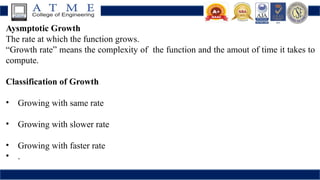
  • 30. Aysmptotic Growth The rate at which the function grows. “Growth rate” means the complexity of the function and the amout of time it takes to compute. Classification of Growth • Growing with same rate • Growing with slower rate • Growing with faster rate • .
  • 31. Asymptotic Notations and Basic Efficiency Classes Asymptotic notation is a notation, which is used mailnly used to represent the time complexities of the algorithms. The efficiency analysis framework concentrates on the order of growth of an algorithm To compare and rank such orders of growth, computer scientists use three notations, they are:  • O - Big oh notation - aymptotic Less Than” (Slower rate) • Ω - Big omega notation - “greater than” (faster rate) • Θ - Big theta notation - “Eqality” (same) Let t(n) and g(n) be any nonnegative functions defined on the set of natural numbers. The algorithm’s running time t(n) usually indicated by its basic operation count C(n), and g(n): eg functions. where g(n) = n2 .
  • 32. i) O - Big oh notation A function t(n) is said to be in O(g(n)), denoted t (n) O(g(n)), if t (n) is bounded above ∈ by some constant multiple of g(n) for all large n, i.e., if there exist some positive constant c and some nonnegative integer n0 such that: t (n) ≤ cg(n) for all n ≥ n0 Where t(n) and g(n) are nonnegative functions defined on the set of natural numbers. O = Asymptotic upper bound = Useful for worst case analysis. FIG 2.1 Big-oh notation: t (n) O(g(n)). ∈
  • 33. Since, the definition gives us a lot of freedom in choosing specific values for constants c and n0. We have c=101 and n0=5
  • 34. (ii) Ω - Big omega notation A function t(n) is said to be in Ω(g(n)), denoted t(n) Ω(g(n)), if t(n) is bounded below by ∈ some positive constant multiple of g(n) for all large n, i.e., if there exist some positive constant c and some nonnegative integer n0 such that t (n) ≥ cg(n) for all n ≥ n0. Where t(n) and g(n) are nonnegative functions defined on the set of natural numbers. Ω = Asymptotic lower bound = Useful for best case analysis = Loose bound
  • 35. Prove the assertions n3 +10n2 +4n+2 Ω (n ∈ 2 ). Proof: n3 +10n2 +4n+2 ≥ n2 (for all n ≥ 0) i.e., by definition t(n) ≥ cg(n), where c=1 and n0=0
  • 36. (iii) Θ - Big theta notation A function t(n) is said to be in Θ(g(n)), denoted t(n) Θ(g(n)), if t(n) is bounded both above ∈ and below by some positive constant multiples of g(n) for all large n, i.e., if there exist some positive constants c1 and c2 and some nonnegative integer n0 such that c2g(n) ≤ t (n) ≤ c1g(n) for all n ≥ n0. Where t(n) and g(n) are nonnegative functions defined on the set of natural numbers. Θ = Asymptotic tight bound = Useful for average case analysis Big-theta notation: t (n) ∈ Θ(g(n)).
  • 38. MATHEMATICALANALYSIS FOR RECURSIVE ALGORITHMS General Plan for Analyzing the Time Efficiency of Recursive Algorithms 1. Decide on a parameter (or parameters) indicating an input’s size. 2. Identify the algorithm’s basic operation. 3. Check whether the number of times the basic operation is executed can vary on different inputs of the same size; if it can, the worst-case, average-case, and best-case efficiencies must be investigated separately. 4. Set up a recurrence relation, with an appropriate initial condition, for the number of times the basic operation is executed. 5. Solve the recurrence or, at least, ascertain the order of growth of its solution.
  • 39. EXAMPLE 1: Compute the factorial function F(n) = n! for an arbitrary nonnegative integer n. Since n!= 1•. . . . • (n − 1) • n = (n − 1)! • n, for n ≥ 1 and 0!= 1 by definition, we can compute F(n) = F(n − 1) • n with the following recursive algorithm. ALGORITHM F(n) //Computes n! recursively //Input: A nonnegative integer n //Output: The value of n! if n = 0 return 1 else return F(n − 1) * n
  • 40. Tower of Hanoi Problem • In this problem, we have n disks of different sizes and three pegs. • Initially, all the disks are on the first peg in order of size, the largest on the bottom and the smallest on top. • The goal is to move all the disks to the third peg, using the second one as an auxiliary if necessary. • We can move only one disk at a time, and it is forbidden to place a larger disk on top of a smaller one.
  • 41. Example 2: The Tower of Hanoi Puzzle 1 2 3 Recurrence for number of moves:
  • 43. Solving recurrence for number of moves
  • 44. n- 1 n- 1 n- 2 n- 2 n- 2 n- 2 1 1 1 .. .. .. 2 1 2 1 1 1 2 1 2 Tree of calls for the Tower of Hanoi Puzzle n
  • 45. MATHEMATICALANALYSIS FOR NON-RECURSIVE ALGORITHMS General Plan for Analyzing the Time Efficiency of Nonrecursive Algorithms 1. Decide on a parameter (or parameters) indicating an input’s size. 2. Identify the algorithm’s basic operation (in the innermost loop). 3. Check whether the number of times the basic operation is executed depends only on the size of an input. If it also depends on some additional property, the worst-case, average-case, and, if necessary, best-case efficiencies have to be investigated separately. 4. Set up a sum expressing the number of times the algorithm’s basic operation is executed. 5. Using standard formulas and rules of sum manipulation either find a closed form formula for the count or at the least, establish its order of growth.
  • 46. EXAMPLE 1: Consider the problem of finding the value of the largest element in a list of n numbers. Assume that the list is implemented as an array for simplicity. ALGORITHM MaxElement(A[0..n − 1]) //Determines the value of the largest element in a given array //Input: An array A[0..n − 1] of real numbers //Output: The value of the largest element in A maxval ←A[0] for i ←1 to n − 1 do if A[i]>maxval maxval←A[i] return maxval
  • 48. Analysis 1. Input parameter : 3. 2. Basic operation: Comparison A[i] > max 4.
  • 49. Example 2: Element uniqueness problem
  • 50. Analysis A[i] == A[j] 1. Input parameter is input size n 2. Basic operation: Comparison 3. 4. Є O(n2)
  • 51. BRUTE FORCE APPROACHES Module 1- Chapt 3 Mrs. Madhu Nagaraj Assistant Professor Dept of CSE-Data Science ATMECE
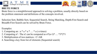
  • 52. BRUTE FORCE Brute force is a straightforward approach to solving a problem, usually directly based on the problem statement and definitions of the concepts involved. Selection Sort, Bubble Sort, Sequential Search, String Matching, Depth-First Search and Breadth-First Search can be solved by Brute Force. Examples: 1. Computing an : a * a * a * … * a ( n times) 2. Computing n! : The n! can be computed as n*(n-1)* … *3*2*1 3. Multiplication of two matrices : C=AB 4. Searching a key from list of elements (Sequential search)
  • 53. Advantages: 1. Brute force is applicable to a very wide variety of problems. 2. It is very useful for solving small size instances of a problem, even though it is inefficient. 3. The brute-force approach yields reasonable algorithms of at least some practical value with no limitation on instance size for sorting, searching, and string matching. Selection Sort ALGORITHM SelectionSort(A[0..n − 1]) //Sorts a given array by selection sort //Input: An array A[0..n − 1] of orderable elements //Output: Array A[0..n − 1] sorted in nondecreasing order for i ← 0 to n − 2 do min ← i for j ← i + 1 to n − 1 do if A[j ]<A[min] min ← j swap A[i] and A[min]
  • 54. The analysis of selection sort is straightforward. The input size is given by the number of elements n; the basic operation is the key comparison A[j ]<A[min]. The number of times it is executed depends only on the array size and is given by the following sum: selection sort is a O(n2 ) algorithm for best case. however, that the number of key swaps is only O(n). Worst case case is also O(n2 )
  • 55. Bubble Sort ALGORITHM BubbleSort(A[0..n − 1]) //Sorts a given array by bubble sort //Input: An array A[0..n − 1] of orderable elements //Output: Array A[0..n − 1] sorted in nondecreasing order for i ← 0 to n − 2 do for j ← 0 to n − 2 − i do if A[j + 1]<A[j ] swap A[j ] and A[j + 1] The number of key comparisons for the bubble-sort version given above is the same for all arrays of size n; it is obtained by a sum that is almost identical to the sum for selection sort:
  • 56. Advantages of Bubble Sort • Easily understandable. • Does not necessitates any extra memory. • The code can be written easily for this algorithm. • Minimal space requirement than that of other sorting algorithms. Disadvantages of Bubble Sort • It does not work well when we have large unsorted lists, and it necessitates more resources that end up taking so much of time. • It is only meant for academic purposes, not for practical implementations. • It involves the n2 order of steps to sort an algorithm.
  • 57. Sequential Serach ALGORITHM SequentialSearch2(A[0..n], K) //Implements sequential search with a search key as a sentinel //Input: An array A of n elements and a search key K //Output: The index of the first element in A[0..n − 1] whose value is // equal to K or −1 if no such element is found A[n]←K i ←0 while A[i] = K do i ←i + 1 if i < n return i else return −1
  • 58. Algorithm for Linear Search: The algorithm for linear search can be broken down into the following steps: 1. Start: Begin at the first element of the collection of elements. 2. Compare: Compare the current element with the desired element. 3. Found: If the current element is equal to the desired element, return true or index to the current element. 4. Move: Otherwise, move to the next element in the collection. 5. Repeat: Repeat steps 2-4 until we have reached the end of collection. 6. Not found: If the end of the collection is reached without finding the desired element, return that the desired element is not in the array.
  • 59. Advantages of Linear Search: • Linear search can be used irrespective of whether the array is sorted or not. It can be used on arrays of any data type. • Does not require any additional memory. • It is a well-suited algorithm for small datasets. Disadvantages of Linear Search: • Linear search has a time complexity of O(N)(Worst Case), which in turn makes it slow for large datasets. • Not suitable for large arrays. When to use Linear Search? • When we are dealing with a small dataset. • When you are searching for a dataset stored in contiguous memory.
  • 60. Brute-Force String Matching pattern: a string of m characters to search for text: a (longer) string of n characters to search in problem: find first substring in text that matches pattern Brute-force: Scan text LR, compare chars, looking for pattern, Step 1 Align pattern at beginning of text Step 2 Moving from left to right, compare each character of pattern to the corresponding character in text until - all characters are found to match (successful search); - or a mismatch is detected Step 3 While pattern is not found and the text is not yet exhausted, realign pattern one position to the right and repeat Step 2
  • 61. Brute-Force String Matching ALGORITHM BruteForceStringMatch(T [0..n − 1], P[0..m − 1]) //Implements brute-force string matching //Input: An array T [0..n − 1] of n characters representing a text and // an array P[0..m − 1] of m characters representing a pattern //Output: The index of the first character in the text that starts a // matching substring or −1 if the search is unsuccessful for i ←0 to n − m do j ←0 while j <m and P[j ]= T [i + j ] do j ←j + 1 if j = m return i return −1 The Time Complexity of the Brute Force Algorithm is O(MXN), where M denotes the length of the text and N denotes the length of the pattern.