This document provides an overview of the Linux operating system. It discusses that Linux is an open-source, multi-user operating system that can run on 32-bit or 64-bit hardware. It then describes some key features of Linux like portability, security, and its hierarchical file system. The document also outlines the architecture of Linux, including its hardware layer, kernel, shell, and utilities. It compares Linux to Unix and Windows, noting Linux is free while Unix is not and that Linux supports multi-tasking better than Windows. Finally, it lists some advantages like free/open-source nature and stability as well as disadvantages such as lack of standard edition and less gaming support.
Everything about OOPs (Object-oriented programming) in this slide we cover the all details about object-oriented programming using C++. we also discussed why C++ is called a subset of C.
This document provides information about loop statements in programming. It discusses the different parts of a loop, types of loops including while, for, and do-while loops. It also covers nested loops and jump statements like break and continue. Examples are given for each loop type. The document concludes with multiple choice and program-based questions as exercises.
This presentation provides an overview of an e-learning management system. It discusses the objectives of providing a user-friendly environment for incremental learning. It analyzes the functional requirements for admins, teachers, and students, as well as non-functional requirements like security, maintainability, and scalability. Sequence diagrams and class diagrams are presented, as well as use case diagrams for each user type. The conclusion states that the system will automate the manual process and enable long-term storage and easy access to information.
The document discusses cyber crime in Nepal. It defines cyber crime and provides examples such as social media related crimes, piracy, fake profiles, threatening emails, website hacking, and unauthorized access. The document notes that cyber crime is a growing problem in Nepal and outlines the types of cyber crimes occurring there such as social media crimes, piracy, fake marketing, threatening emails, website hacking, unauthorized access, and restricted online businesses. It also discusses the effects of cyber crimes and Nepal's efforts to combat cyber crimes.
Introduction, features of women entrepreneurship, why women become entrepreneurs, qualities, tips for women entrepreneurs, facilitating factors, opportunities, challenges, problems, remedial measures, steps taken by government, training programs, supporting agencies and about some famous women entrepreneurs
Binary trees are a data structure where each node has at most two children. A binary tree node contains data and pointers to its left and right child nodes. Binary search trees are a type of binary tree where nodes are organized in a manner that allows for efficient searches, insertions, and deletions of nodes. The key operations on binary search trees are searching for a node, inserting a new node, and deleting an existing node through various algorithms that traverse the tree. Common traversals of binary trees include preorder, inorder, and postorder traversals.
it's just overview to how make srs of any software . In that ppt all function of make my trip.com are not shown. it just give the overview of all function of make my trip.com software.
Algorithms Lecture 1: Introduction to AlgorithmsMohamed Loey
We will discuss the following: Algorithms, Time Complexity & Space Complexity, Algorithm vs Pseudo code, Some Algorithm Types, Programming Languages, Python, Anaconda.
This document discusses various sorting algorithms and their complexities. It begins by defining an algorithm and complexity measures like time and space complexity. It then defines sorting and common sorting algorithms like bubble sort, selection sort, insertion sort, quicksort, and mergesort. For each algorithm, it provides a high-level overview of the approach and time complexity. It also covers sorting algorithm concepts like stable and unstable sorting. The document concludes by discussing future directions for sorting algorithms and their applications.
This document describes binary search and provides an example of how it works. It begins with an introduction to binary search, noting that it can only be used on sorted lists and involves comparing the search key to the middle element. It then provides pseudocode for the binary search algorithm. The document analyzes the time complexity of binary search as O(log n) in the average and worst cases. It notes the advantages of binary search are its efficiency, while the disadvantage is that the list must be sorted. Applications mentioned include database searching and solving equations.
This document presents selection sort, an in-place comparison sorting algorithm. It works by dividing the list into a sorted part on the left and unsorted part on the right. It iterates through the list, finding the smallest element in the unsorted section and swapping it into place. This process continues until the list is fully sorted. Selection sort has a time complexity of O(n^2) in all cases. While it requires no extra storage, it is inefficient for large lists compared to other algorithms.
This document discusses the complexity of algorithms and the tradeoff between algorithm cost and time. It defines algorithm complexity as a function of input size that measures the time and space used by an algorithm. Different complexity classes are described such as polynomial, sub-linear, and exponential time. Examples are given to find the complexity of bubble sort and linear search algorithms. The concept of space-time tradeoffs is introduced, where using more space can reduce computation time. Genetic algorithms are proposed to efficiently solve large-scale construction time-cost tradeoff problems.
Data Structures and Algorithm - Module 1.pptxEllenGrace9
This document provides an introduction to data structures and algorithms from instructor Ellen Grace Porras. It defines data structures as ways of organizing data to allow for efficient operations. Linear data structures like arrays, stacks, and queues arrange elements sequentially, while non-linear structures like trees and graphs have hierarchical relationships. The document discusses characteristics of good data structures and algorithms, provides examples of common algorithms, and distinguishes between linear and non-linear data structures. It aims to explain the fundamentals of data structures and algorithms.
This document provides an overview of trees as a non-linear data structure. It begins by discussing how trees are used to represent hierarchical relationships and defines some key tree terminology like root, parent, child, leaf, and subtree. It then explains that a tree consists of nodes connected in a parent-child relationship, with one root node and nodes that may have any number of children. The document also covers tree traversal methods like preorder, inorder, and postorder traversal. It introduces binary trees and binary search trees, and discusses operations on BSTs like search, insert, and delete. Finally, it provides a brief overview of the Huffman algorithm for data compression.
The document discusses divide and conquer algorithms. It describes divide and conquer as a design strategy that involves dividing a problem into smaller subproblems, solving the subproblems recursively, and combining the solutions. It provides examples of divide and conquer algorithms like merge sort, quicksort, and binary search. Merge sort works by recursively sorting halves of an array until it is fully sorted. Quicksort selects a pivot element and partitions the array into subarrays of smaller and larger elements, recursively sorting the subarrays. Binary search recursively searches half-intervals of a sorted array to find a target value.
Command-line arguments are given after the name of the program in command-line shell of Operating Systems.
To pass command line arguments, we typically define main() with two arguments : first argument is the number of command line arguments and second is list of command-line arguments.
This document provides an overview of algorithm analysis. It discusses how to analyze the time efficiency of algorithms by counting the number of operations and expressing efficiency using growth functions. Different common growth rates like constant, linear, quadratic, and exponential are introduced. Examples are provided to demonstrate how to determine the growth rate of different algorithms, including recursive algorithms, by deriving their time complexity functions. The key aspects covered are estimating algorithm runtime, comparing growth rates of algorithms, and using Big O notation to classify algorithms by their asymptotic behavior.
PPT on Analysis Of Algorithms.
The ppt includes Algorithms,notations,analysis,analysis of algorithms,theta notation, big oh notation, omega notation, notation graphs
Hashing is the process of converting a given key into another value. A hash function is used to generate the new value according to a mathematical algorithm. The result of a hash function is known as a hash value or simply, a hash.
The document discusses algorithm analysis and asymptotic notation. It defines algorithm analysis as comparing algorithms based on running time and other factors as problem size increases. Asymptotic notation such as Big-O, Big-Omega, and Big-Theta are introduced to classify algorithms based on how their running times grow relative to input size. Common time complexities like constant, logarithmic, linear, quadratic, and exponential are also covered. The properties and uses of asymptotic notation for equations and inequalities are explained.
This document provides an introduction to asymptotic analysis of algorithms. It discusses analyzing algorithms based on how their running time increases with the size of the input problem. The key points are:
- Algorithms are compared based on their asymptotic running time as the input size increases, which is more useful than actual running times on a specific computer.
- The main types of analysis are worst-case, best-case, and average-case running times.
- Asymptotic notations like Big-O, Omega, and Theta are used to classify algorithms based on their rate of growth as the input increases.
- Common orders of growth include constant, logarithmic, linear, quadratic, and exponential time.
The document discusses the divide and conquer algorithm design technique. It begins by explaining the basic approach of divide and conquer which is to (1) divide the problem into subproblems, (2) conquer the subproblems by solving them recursively, and (3) combine the solutions to the subproblems into a solution for the original problem. It then provides merge sort as a specific example of a divide and conquer algorithm for sorting a sequence. It explains that merge sort divides the sequence in half recursively until individual elements remain, then combines the sorted halves back together to produce the fully sorted sequence.
This document discusses different searching methods like sequential, binary, and hashing. It defines searching as finding an element within a list. Sequential search searches lists sequentially until the element is found or the end is reached, with efficiency of O(n) in worst case. Binary search works on sorted arrays by eliminating half of remaining elements at each step, with efficiency of O(log n). Hashing maps keys to table positions using a hash function, allowing searches, inserts and deletes in O(1) time on average. Good hash functions uniformly distribute keys and generate different hashes for similar keys.
Linked lists are linear data structures where each node contains a data field and a pointer to the next node. There are two types: singly linked lists where each node has a single next pointer, and doubly linked lists where each node has next and previous pointers. Common operations on linked lists include insertion and deletion which have O(1) time complexity for singly linked lists but require changing multiple pointers for doubly linked lists. Linked lists are useful when the number of elements is dynamic as they allow efficient insertions and deletions without shifting elements unlike arrays.
This document discusses linked lists and polynomials represented as linked lists. It provides details on singly linked lists, including how to implement insertion and deletion of nodes. It also describes how to represent stacks and queues as dynamically linked lists. Finally, it discusses representing polynomials using arrays or linked lists, and how to perform addition and multiplication of polynomials in each representation.
This document discusses algorithms and their analysis. It defines an algorithm as a set of unambiguous instructions to solve a problem with inputs and outputs. Good algorithms have well-defined steps, inputs, outputs, and terminate in a finite number of steps. Common algorithm analysis methods include calculating time and space complexity using asymptotic notations like Big-O. Pseudocode and flowcharts are commonly used to represent algorithms. Asymptotic analysis determines an algorithm's best, average, and worst case running times.
The document discusses algorithms and their analysis. It defines an algorithm as a step-by-step procedure to solve a problem and get a desired output. Key aspects of algorithms discussed include their time and space complexity, asymptotic analysis to determine best, average, and worst case running times, and common asymptotic notations like Big O that are used to analyze algorithms. Examples are provided to demonstrate how to determine the time and space complexity of different algorithms like those using loops, recursion, and nested loops.
The document discusses algorithms, including their definition, common types of algorithms, properties of algorithms, and how to write algorithms. It provides an example algorithm to add two numbers and explains how to analyze algorithms for efficiency in terms of time and space complexity. Time complexity represents the running time of an algorithm, while space complexity represents the memory required.
This document defines and explains algorithms and their analysis. It begins by defining an algorithm as a step-by-step procedure to solve a problem from input to output. Characteristics of algorithms include being unambiguous, having defined inputs/outputs, terminating in a finite number of steps, and being independent of programming language. The document then discusses analyzing algorithms to determine time and space complexity before and after implementation. Common asymptotic notations like Big-O, Omega, and Theta are explained. Finally, the document reviews common data structures like linked lists, stacks, queues, and trees.
The document provides an introduction to data structures and algorithms analysis. It discusses that a program consists of organizing data in a structure and a sequence of steps or algorithm to solve a problem. A data structure is how data is organized in memory and an algorithm is the step-by-step process. It describes abstraction as focusing on relevant problem properties to define entities called abstract data types that specify what can be stored and operations performed. Algorithms transform data structures from one state to another and are analyzed based on their time and space complexity.
The document provides an introduction to algorithms and their analysis. It defines an algorithm and lists its key criteria. It discusses different representations of algorithms including flowcharts and pseudocode. It also outlines the main areas of algorithm analysis: devising algorithms, validating them, analyzing performance, and testing programs. Finally, it provides examples of algorithms and their analysis including calculating time complexity based on counting operations.
This document provides an overview of data structures and algorithms. It discusses key concepts like interfaces, implementations, time complexity, space complexity, asymptotic analysis, and common control structures. Some key points:
- A data structure organizes data to allow for efficient operations. It has an interface defining operations and an implementation defining internal representation.
- Algorithm analysis considers best, average, and worst case time complexities using asymptotic notations like Big O. Space complexity also measures memory usage.
- Common control structures include sequential, conditional (if/else), and repetitive (loops) structures that control program flow based on conditions.
This document introduces algorithms and their basics. It defines an algorithm as a step-by-step procedure to solve a problem and get the desired output. Algorithms can be implemented in different programming languages. Common algorithm categories include search, sort, insert, update, and delete operations on data structures. An algorithm must be unambiguous, have well-defined inputs and outputs, terminate in a finite number of steps, and be feasible with available resources. The document also discusses how to write algorithms, analyze their complexity, and commonly used asymptotic notations like Big-O, Omega, and Theta.
The document discusses stacks and queues as linear data structures. A stack follows LIFO (last in first out) where the last element inserted is the first removed. Common stack operations are push to insert and pop to remove elements. Stacks can be implemented using arrays or linked lists. A queue follows FIFO (first in first out) where the first element inserted is the first removed. Common queue operations are enqueue to insert and dequeue to remove elements. Queues can also be implemented using arrays or linked lists. Circular queues and priority queues are also introduced.
The document discusses stacks and queues as linear data structures. A stack follows LIFO (last in first out) where the last element inserted is the first to be removed. Common stack operations are push to add an element and pop to remove an element. Stacks can be implemented using arrays or linked lists. A queue follows FIFO (first in first out) where the first element inserted is the first to be removed. Common queue operations are enqueue to add an element and dequeue to remove an element. Queues can also be implemented using arrays or linked lists. Circular queues and priority queues are also discussed briefly.
An algorithm is a well-defined set of steps to solve a problem in a finite amount of time. The complexity of an algorithm measures the time and space required for inputs of different sizes. Time complexity indicates the running time, while space complexity measures storage usage. Analyzing algorithms involves determining their asymptotic worst-case, best-case, and average-case time complexities using notations like Big-O, Omega, and Theta. This provides insights into an algorithm's efficiency under different conditions.
An algorithm is a well-defined set of steps to solve a problem in a finite amount of time. The complexity of an algorithm measures the time and space required for inputs of different sizes. Time complexity indicates the running time, while space complexity measures storage usage. These complexities can be analyzed before and after implementation using asymptotic notations like Big-O, Omega, and Theta to determine worst-case, best-case, and average-case efficiencies. Proper algorithm design considers factors like understandability, efficiency, and resource usage.
This document provides an overview of algorithms including definitions, characteristics, design, and analysis. It defines an algorithm as a finite step-by-step procedure to solve a problem and discusses their key characteristics like input, definiteness, effectiveness, finiteness, and output. The document outlines the design of algorithms using pseudo-code and their analysis in terms of time and space complexity using asymptotic notations like Big O, Big Omega, and Big Theta. Examples are provided to illustrate linear search time complexity and the use of different notations to determine algorithm efficiency.
This slides contains assymptotic notations, recurrence relation like subtitution method, iteration method, master method and recursion tree method and sorting algorithms like merge sort, quick sort, heap sort, counting sort, radix sort and bucket sort.
The document discusses algorithms and their analysis. It defines an algorithm as a sequence of unambiguous steps to solve a problem within a finite time. Characteristics of algorithms include being unambiguous, having inputs/outputs, and terminating in finite time. Algorithm analysis involves determining theoretical and empirical time and space complexity as input size increases. Time complexity is analyzed by counting basic operations, while space complexity considers fixed and variable memory usage. Worst, best, and average cases analyze how efficiency varies with different inputs. Asymptotic analysis focuses on long-term growth rates to compare algorithms.
The document outlines the objectives, outcomes, teaching scheme, and evaluation methods for an advanced data structures and algorithms course. It describes assessing students through in-semester exams, innovative exams where students implement solutions to problems, and end-semester exams. The document also provides examples of potential research projects and outlines the course syllabus, including modules on complexity analysis, common algorithms like search and sort, and analysis of algorithm performance.
This document discusses algorithmic efficiency and complexity. It begins by defining an algorithm as a step-by-step procedure for solving a problem in a finite amount of time. It then discusses estimating the complexity of algorithms, including asymptotic notations like Big O, Big Omega, and Theta that are used to describe an algorithm's time and space complexity. The document provides examples of time and space complexity for common algorithms like searching and sorting. It concludes by emphasizing the importance of analyzing algorithms to minimize their cost and maximize efficiency.
How to use nRF24L01 module with ArduinoCircuitDigest
Learn how to wirelessly transmit sensor data using nRF24L01 and Arduino Uno. A simple project demonstrating real-time communication with DHT11 and OLED display.
The Fluke 925 is a vane anemometer, a handheld device designed to measure wind speed, air flow (volume), and temperature. It features a separate sensor and display unit, allowing greater flexibility and ease of use in tight or hard-to-reach spaces. The Fluke 925 is particularly suitable for HVAC (heating, ventilation, and air conditioning) maintenance in both residential and commercial buildings, offering a durable and cost-effective solution for routine airflow diagnostics.
ADVXAI IN MALWARE ANALYSIS FRAMEWORK: BALANCING EXPLAINABILITY WITH SECURITYijscai
With the increased use of Artificial Intelligence (AI) in malware analysis there is also an increased need to
understand the decisions models make when identifying malicious artifacts. Explainable AI (XAI) becomes
the answer to interpreting the decision-making process that AI malware analysis models use to determine
malicious benign samples to gain trust that in a production environment, the system is able to catch
malware. With any cyber innovation brings a new set of challenges and literature soon came out about XAI
as a new attack vector. Adversarial XAI (AdvXAI) is a relatively new concept but with AI applications in
many sectors, it is crucial to quickly respond to the attack surface that it creates. This paper seeks to
conceptualize a theoretical framework focused on addressing AdvXAI in malware analysis in an effort to
balance explainability with security. Following this framework, designing a machine with an AI malware
detection and analysis model will ensure that it can effectively analyze malware, explain how it came to its
decision, and be built securely to avoid adversarial attacks and manipulations. The framework focuses on
choosing malware datasets to train the model, choosing the AI model, choosing an XAI technique,
implementing AdvXAI defensive measures, and continually evaluating the model. This framework will
significantly contribute to automated malware detection and XAI efforts allowing for secure systems that
are resilient to adversarial attacks.
Raish Khanji GTU 8th sem Internship Report.pdfRaishKhanji
This report details the practical experiences gained during an internship at Indo German Tool
Room, Ahmedabad. The internship provided hands-on training in various manufacturing technologies, encompassing both conventional and advanced techniques. Significant emphasis was placed on machining processes, including operation and fundamental
understanding of lathe and milling machines. Furthermore, the internship incorporated
modern welding technology, notably through the application of an Augmented Reality (AR)
simulator, offering a safe and effective environment for skill development. Exposure to
industrial automation was achieved through practical exercises in Programmable Logic Controllers (PLCs) using Siemens TIA software and direct operation of industrial robots
utilizing teach pendants. The principles and practical aspects of Computer Numerical Control
(CNC) technology were also explored. Complementing these manufacturing processes, the
internship included extensive application of SolidWorks software for design and modeling tasks. This comprehensive practical training has provided a foundational understanding of
key aspects of modern manufacturing and design, enhancing the technical proficiency and readiness for future engineering endeavors.
Passenger car unit (PCU) of a vehicle type depends on vehicular characteristics, stream characteristics, roadway characteristics, environmental factors, climate conditions and control conditions. Keeping in view various factors affecting PCU, a model was developed taking a volume to capacity ratio and percentage share of particular vehicle type as independent parameters. A microscopic traffic simulation model VISSIM has been used in present study for generating traffic flow data which some time very difficult to obtain from field survey. A comparison study was carried out with the purpose of verifying when the adaptive neuro-fuzzy inference system (ANFIS), artificial neural network (ANN) and multiple linear regression (MLR) models are appropriate for prediction of PCUs of different vehicle types. From the results observed that ANFIS model estimates were closer to the corresponding simulated PCU values compared to MLR and ANN models. It is concluded that the ANFIS model showed greater potential in predicting PCUs from v/c ratio and proportional share for all type of vehicles whereas MLR and ANN models did not perform well.
ELectronics Boards & Product Testing_Shiju.pdfShiju Jacob
This presentation provides a high level insight about DFT analysis and test coverage calculation, finalizing test strategy, and types of tests at different levels of the product.
its all about Artificial Intelligence(Ai) and Machine Learning and not on advanced level you can study before the exam or can check for some information on Ai for project
2. An algorithm is finite set of instructions which is followed, accomplish
particular task or it is a sequential steps of instruction of programs.
An algorithm is a sequence of computational steps that transform the input
into the output.
An algorithm is sequence of operations performed on data that have to be
organized in data structure.
3. Every algorithm must satisfy the following criteria-
1. Input- There are zero or more quantities which are externally
supplied.
2. Output – At least one quantity is produced.
3. Definiteness – Each instruction must be clear and easy to understand.
4. Finiteness- Algorithm will terminate after finite number of steps.
5. Effectiveness- Every instruction must be roughly work out using
pencil and paper. More effectively generated.
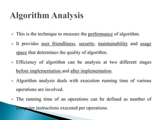
4. This is the technique to measure the performance of algorithm.
It provides user friendliness, security, maintainability and usage
space that determines the quality of algorithm.
Efficiency of algorithm can be analysis at two different stages
before implementation and after implementation.
Algorithm analysis deals with execution running time of various
operations are involved.
The running time of an operations can be defined as number of
computer instructions executed per operations.
5. 1. Priori analysis-
This is the theoretical analysis of algorithm before
implementation. Efficiency of algorithm measured by speed,
constant have no effects on implementation.
2. Posterior analysis-
The selected algorithm implemented using programming
language. This is executed on target computer machine. In this
analysis actual statistics like running time and space calculated after
implementation.
6. Algorithms help us to understand scalability.
Performance often draws the line between what is feasible and what is impossible.
Algorithmic mathematics provides a language for talking about program behavior.
The lessons of program performance generalize to other computing resources.
Modularity, Correctness, Maintainability, Correctness, Robustness, User
friendliness, Programming time, Simplicity, Reliability etc. Its important for good
performance.
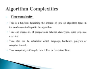
7. 1. Time complexity-
This is a function describing the amount of time an algorithm takes in
terms of amount of input to the algorithm.
Time can means no. of comparisons between data types, inner loops are
executed.
Time also can be calculated which language, hardware, program or
compiler is used.
Time complexity = Compile time + Run or Execution Time.
8. 2. Space Complexity-
Space complexity of an algorithm represents amount of memory space
required by the algorithm in its life cycle.
Two types of spaces are required-
Fixed part- It required to store certain data and variables that are
independent size of problem. For e.g. Constants, Program size etc.
Variable part- It required by variables whose size depends on size of
problem. For e.g. Dynamic memory allocation.
9. Algorithm: SUM(A,B)
Step 1 - START
Step 2 - C <- A+B+10
Step 3 – Stop 1
Space complexity S(P) of any algorithm P is S(P) = C+SP(I). Where, C is
fixed part and S(I) is variable part of algorithm.
There are three variables A,B,C and Constant.
Space depends on data types of given variables and constant types of data.
10. Asymptotic analysis of an algorithm refers to define the mathematical
foundation of its run time performance. For this purpose we used Best,
Average and Worst cases.
Asymptotic Notations-
1. Big O Notation, O –
The notation O(n) is the way to express the upper bound of an algorithm
running time. Its measure the worst case time complexity or longest
amount of time an algorithm can possibly take to complete.
f(n) (- O(g(n))
11. 2. Omega Notation, Ω –
The notation Ω(n) is the way to express lower bound of an algorithm running
time. It measure the best case time or minimum amount of time an algorithm
can possible take to complete.
f(n) (- Ω(g(n))
3. Theta Notation, θ –
The notation θ(n) is the formal way to express both the lower bound and
upper bound of an algorithm running time can possible take to complete.
f(n) (- θ(g(n))
13. 1. Best case analysis-
Best case is that input to the algorithm which takes minimum time for
execution of it.
Example - Binary Search algorithm
1 2 3 4 5 6 7 8 9
Best case to search element at first position.
It required O(1) time.
14. 2. Average case analysis-
For average case analysis all possible sequence of size ‘n’ are input to the
algorithm and average asymptotic time of algorithm is computed.
Example - Binary Search algorithm
1 2 3 4 5 6 7 8 9
All elements of sorted array of size ‘n’ are searched one by one and total
number of comparisons are computed.
Average computation time = Total time/2.
It requires O(log n) time.
15. 3. Worst case analysis-
Worst case is that input to the algorithm which takes maximum time for
execution of it.
Example - Binary Search algorithm
1 2 3 4 5 6 7 8 9
Worst case search the last element of the list in O(n) time is required. If the
element is absent then O(log n) time is required.
16. Input
1 ms
2 ms
3 ms
4 ms
5 ms
A B C D E F G
worst-case
best-case
}average-case?
17. 1. O(1) – Constant eg. Doing a null check
2. O(n) – Logarithmic eg. Searching sorted data
3. O(n) – Linear eg. Adding values in data set
4. O(n log n) – Linearithmic eg. Quick sort
5. O(n2) – Quadratic eg. Two nested loops
6. O(n^k) – Polynomial eg. Calculations of polynomials
7. O(2n) – Exponential eg. Brute force attacking a password
8. O(n!) – Factorial eg. Calculate Fibonacci series
19. The key take away here is that if you are working with large
datasets you need to be careful when selecting proper data
structure, algorithms you use.