


![Worst Case Analysis (Usually Done)
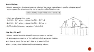
Calculate upper bound on running time of an algorithm.
The case that causes maximum number of operations to be executed.
For Linear Search, the worst case happens when the element to be searched is not present in the array. When x is not present, the
search() functions compares it with all the elements of arr[] one by one. Therefore, the worst case time complexity of linear search
would be Θ(n).
Most of the time its preferred, we guarantee an upper bound on the running time of an algorithm which is good information.
Average Case Analysis (Sometimes done)
We take all possible inputs and calculate computing time for all of the inputs. Sum all the calculated values and divide the sum by total
number of inputs.
For the linear search problem, let us assume that all cases are uniformly distributed. So we sum all the cases and divide the sum by
(n+1).
Following is the value of average case time complexity.
Rarely done as it’s not easy to do in most of the practical cases. We must know the mathematical distribution of all possible inputs
Average Case Time = = = Θ(n)](https://image.slidesharecdn.com/analysisofalgorithms-191004205322/85/Analysis-of-algorithms-4-320.jpg)


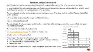
![ In recurrence tree method, we calculate total work done.
If the work done at leaves is polynomially more, then leaves are the dominant part, and our result becomes the work
done at leaves (Case 1).
If work done at leaves and root is asymptotically same, then our result becomes height multiplied by work done at
any level (Case 2).
If work done at root is asymptotically more, then our result becomes work done at root (Case 3).
Examples of some standard algorithms whose time complexity can be evaluated using Master Method
Merge Sort: T(n) = 2T(n/2) + Θ(n). It falls in case 2 as c is 1 and Logba] is also 1. So the solution is Θ(n Logn)
Binary Search: T(n) = T(n/2) + Θ(1). It also falls in case 2 as c is 0 and Logba is also 0. So the solution is Θ(Logn)
Notes:
It is not necessary that a recurrence of the form T(n) = aT(n/b) + f(n) can be solved using Master Theorem.
The given three cases have some gaps between them. For example, the recurrence T(n) = 2T(n/2) + n/Logn
cannot be solved using master method.
Case 2 can be extended for f(n) = Θ(ncLogkn)
If f(n) = Θ(ncLogkn) for some constant k >= 0 and c = Logba, then T(n) = Θ(ncLogk+1n)](https://image.slidesharecdn.com/analysisofalgorithms-191004205322/85/Analysis-of-algorithms-16-320.jpg)


More Related Content
What's hot (20)
Similar to Analysis of algorithms (20)


Recently uploaded (20)


Analysis of algorithms
- 2. Why performance analysis? Imagine a text editor that can load 1000 pages, but can spell check 1 page per minute OR an image editor that takes 1 hour to rotate your image 90 degrees left OR … you get it. If a software feature can not cope with the scale of tasks users need to perform – it is as good as dead. Given two algorithms for a task, how do we find out which one is better? One naive way of doing this is – implement both the algorithms and run the two programs on your computer for different inputs and see which one takes less time. There are many problems with this approach for analysis of algorithms. 1. It might be possible that for some inputs, first algorithm performs better than the second. And for some inputs second performs better. 2. It might also be possible that for some inputs, first algorithm perform better on one machine and the second works better on other machine for some other inputs. Evaluates the performance of an algorithm in terms of input size (we don’t measure the actual running time). We calculate, how does the time (or space) taken by an algorithm increases with the input size. For example, let us consider the search problem (searching a given item) in a sorted array. One way to search is Linear Search (order of growth is linear) and other way is Binary Search (order of growth is logarithmic). Asymptotic Analysis
- 3. To understand how Asymptotic Analysis solves the above mentioned problems in analyzing algorithms, let us say we run the Linear Search on a fast computer and Binary Search on a slow computer. For small values of input array size n, the fast computer may take less time. But, after certain value of input array size, the Binary Search will definitely start taking less time compared to the Linear Search even though the Binary Search is being run on a slow machine. The reason is the order of growth of Binary Search with respect to input size logarithmic while the order of growth of Linear Search is linear. So the machine dependent constants can always be ignored after certain values of input size. Does Asymptotic Analysis always work? Asymptotic Analysis is not perfect, but that’s the best way available for analyzing algorithms. For example, say there are two sorting algorithms that take 1000nLogn and 2nLogn time respectively on a machine. Both of these algorithms are asymptotically same (order of growth is nLogn). So, With Asymptotic Analysis, we can’t judge which one is better as we ignore constants in Asymptotic Analysis. Also, in Asymptotic analysis, we always talk about input sizes larger than a constant value. It might be possible that those large inputs are never given to your software and an algorithm which is asymptotically slower, always performs better for your particular situation. So, you may end up choosing an algorithm that is Asymptotically slower but faster for your software.
- 4. Worst Case Analysis (Usually Done) Calculate upper bound on running time of an algorithm. The case that causes maximum number of operations to be executed. For Linear Search, the worst case happens when the element to be searched is not present in the array. When x is not present, the search() functions compares it with all the elements of arr[] one by one. Therefore, the worst case time complexity of linear search would be Θ(n). Most of the time its preferred, we guarantee an upper bound on the running time of an algorithm which is good information. Average Case Analysis (Sometimes done) We take all possible inputs and calculate computing time for all of the inputs. Sum all the calculated values and divide the sum by total number of inputs. For the linear search problem, let us assume that all cases are uniformly distributed. So we sum all the cases and divide the sum by (n+1). Following is the value of average case time complexity. Rarely done as it’s not easy to do in most of the practical cases. We must know the mathematical distribution of all possible inputs Average Case Time = = = Θ(n)
- 5. Best Case Analysis (Bogus) Calculate lower bound on running time of an algorithm. Case that causes minimum number of operations to be executed. In the linear search problem, the best case occurs when x is present at the first location. The number of operations in the best case is constant (not dependent on n). So time complexity in the best case would be Θ(1). The Best Case analysis is bogus. Guaranteeing a lower bound on an algorithm doesn’t provide any information as in the worst case, an algorithm may take years to run. Conclusion For some algorithms, all the cases are asymptotically same, i.e., there are no worst and best cases. For example, Merge Sort. Merge Sort does Θ(nLogn) operations in all cases. Most of the other sorting algorithms have worst and best cases. For example, in the typical implementation of Quick Sort (where pivot is chosen as a corner element), the worst occurs when the input array is already sorted and the best occur when the pivot elements always divide array in two halves. For insertion sort, the worst case occurs when the array is reverse sorted and the best case occurs when the array is sorted in the same order as output.
- 6. The main idea is to have a measure of efficiency of algorithms that doesn’t depend on machine specific constants, and doesn’t require algorithms to be implemented and time taken by programs to be compared. Asymptotic notations are mathematical tools to represent time complexity of algorithms for asymptotic analysis. Θ Notation: Bounds functions from above and below, so it defines exact asymptotic behavior. A simple way to get Theta notation of an expression is to drop low order terms and ignore leading constants. For example, consider the following expression. 3n3 + 6n2 + 6000 = Θ(n3) Dropping lower order terms is always fine because there will always be a n0 after which Θ(n3) has higher values than Θn2) irrespective of the constants involved. For a given function g(n), we denote Θ(g(n)) is following set of functions. Θ(g(n)) = {f(n): there exist positive constants c1, c2 and n0 such that 0 <= c1*g(n) <= f(n) <= c2*g(n) for all n >= n0} The above definition means, if f(n) is theta of g(n), then the value f(n) is always between c1*g(n) and c2*g(n) for large values of n (n >= n0). The definition of theta also requires that f(n) must be non-negative for values of n greater than n0.
- 7. Big O Notation: Defines an upper bound of an algorithm, it bounds a function only from above. For example, consider the case of Insertion Sort. It takes linear time in best case and quadratic time in worst case. We can safely say that the time complexity of Insertion sort is O(n^2). Note that O(n^2) also covers linear time. If we use Θ notation to represent time complexity of Insertion sort, we have to use two statements for best and worst cases: 1. The worst case time complexity of Insertion Sort is Θ(n^2). 2. The best case time complexity of Insertion Sort is Θ(n). The Big O notation is useful when we only have upper bound on time complexity of an algorithm. Many times we easily find an upper bound by simply looking at the algorithm. O(g(n)) = { f(n): there exist positive constants c and n0 such that 0 <= f(n) <= c*g(n) for all n >= n0}
- 8. Ω Notation: Provides an asymptotic lower bound. Useful when we have lower bound on time complexity of an algorithm. Is the least used notation among all three. For a given function g(n), we denote by Ω(g(n)) the set of functions. Ω (g(n)) = {f(n): there exist positive constants c and n0 such that 0 <= c*g(n) <= f(n) for all n >= n0}. The time complexity of Insertion Sort can be written as Ω(n), but it is not a very useful information about insertion sort, as we are generally interested in worst case and sometimes in average case.
- 9. O(1): Time complexity of a function (or set of statements) is considered as O(1) if it doesn’t contain loop, recursion and call to any other non-constant time function. For example swap() function has O(1) time complexity. A loop or recursion that runs a constant number of times is also considered as O(1). For example the following loop is O(1). O(n): Time Complexity of a loop is considered as O(n) if the loop variables is incremented / decremented by a constant amount. For example following functions have O(n) time complexity.
- 10. O(nc): Time complexity of nested loops is equal to the number of times the innermost statement is executed. For example the following sample loops have O(n2) time complexity. For example Selection sort and Insertion Sort have O(n2) time complexity. O(Logn): Time Complexity of a loop is considered as O(Logn) if the loop variables is divided / multiplied by a constant amount. For example Binary Search(refer iterative implementation) has O(Logn) time complexity. Let us see mathematically how it is O(Log n). The series that we get in first loop is 1, c, c2, c3, … ck. If we put k equals to Logcn, we get cLog c n which is n.
- 11. O(LogLogn): Time Complexity of a loop is considered as O(LogLogn) if the loop variables is reduced / increased exponentially by a constant amount. How to combine time complexities of consecutive loops? When there are consecutive loops, we calculate time complexity as sum of time complexities of individual loops.
- 12. How to calculate time complexity when there are many if, else statements inside loops? Evaluate the situation when values in if-else conditions cause maximum number of statements to be executed. For example, consider the linear search function where we consider the case when element is present at the end or not present at all. When the code is too complex to consider all if-else cases, we can get an upper bound by ignoring if else and other complex control statements. How to calculate time complexity of recursive functions? Time complexity of a recursive function can be written as a mathematical recurrence relation. To calculate time complexity, we must know how to solve recurrences.
- 13. We get running time on an input of size n as a function of n and the running time on inputs of smaller sizes. For example in Merge Sort, to sort a given array, we divide it in two halves and recursively repeat the process for the two halves. Finally we merge the results. Time complexity of Merge Sort can be written as T(n) = 2T(n/2) + cn. There are many other algorithms like Binary Search, Tower of Hanoi, etc. Substitution Method: We make a guess for the solution and then we use mathematical induction to prove the guess is correct or incorrect. Solving Recurrences
- 14. Recurrence Tree Method: In this method, we draw a recurrence tree and calculate the time taken by every level of tree. Finally, we sum the work done at all levels. To draw the recurrence tree, we start from the given recurrence and keep drawing till we find a pattern among levels. The pattern is typically a arithmetic or geometric series.
- 15. Master Method: Master Method is a direct way to get the solution. The master method works only for following type of recurrences or for recurrences that can be transformed to following type. There are following three cases: 1. If f(n) = Θ(nc) where c < Logba then T(n) = Θ(nLog b a) 2. If f(n) = Θ(nc) where c = Logba then T(n) = Θ(ncLog n) 3.If f(n) = Θ(nc) where c > Logba then T(n) = Θ(f(n)) How does this work? Master method is mainly derived from recurrence tree method. If we draw recurrence tree of T(n) = aT(n/b) + f(n), we can see that the work done at root is f(n) and work done at all leaves is Θ(nc) where c is Logba. And the height of recurrence tree is Logbn
- 16. In recurrence tree method, we calculate total work done. If the work done at leaves is polynomially more, then leaves are the dominant part, and our result becomes the work done at leaves (Case 1). If work done at leaves and root is asymptotically same, then our result becomes height multiplied by work done at any level (Case 2). If work done at root is asymptotically more, then our result becomes work done at root (Case 3). Examples of some standard algorithms whose time complexity can be evaluated using Master Method Merge Sort: T(n) = 2T(n/2) + Θ(n). It falls in case 2 as c is 1 and Logba] is also 1. So the solution is Θ(n Logn) Binary Search: T(n) = T(n/2) + Θ(1). It also falls in case 2 as c is 0 and Logba is also 0. So the solution is Θ(Logn) Notes: It is not necessary that a recurrence of the form T(n) = aT(n/b) + f(n) can be solved using Master Theorem. The given three cases have some gaps between them. For example, the recurrence T(n) = 2T(n/2) + n/Logn cannot be solved using master method. Case 2 can be extended for f(n) = Θ(ncLogkn) If f(n) = Θ(ncLogkn) for some constant k >= 0 and c = Logba, then T(n) = Θ(ncLogk+1n)
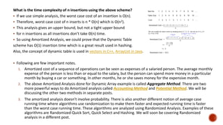
- 17. Used for algorithms where an occasional operation is very slow, but most of the other operations are faster. In Amortized Analysis, we analyze a sequence of operations and guarantee a worst case average time which is lower than the worst case time of a particular expensive operation. The example data structures whose operations are analyzed using Amortized Analysis are Hash Tables, Disjoint Sets and Splay Trees. Let us consider an example of a simple hash table insertions. How do we decide table size? There is a trade-off between space and time, if we make hash-table size big, search time becomes fast, but space required becomes high. The solution to this trade-off problem is to use Dynamic Table (or Arrays). The idea is to increase size of table whenever it becomes full. Following are the steps to follow when table becomes full. 1) Allocate memory for a larger table of size, typically twice the old table. 2) Copy the contents of old table to new table. 3) Free the old table. If the table has space available, we simply insert new item in available space. Amortized Analysis Introduction
- 18. What is the time complexity of n insertions using the above scheme? If we use simple analysis, the worst case cost of an insertion is O(n). Therefore, worst case cost of n inserts is n * O(n) which is O(n2). This analysis gives an upper bound, but not a tight upper bound for n insertions as all insertions don’t take Θ(n) time. So using Amortized Analysis, we could prove that the Dynamic Table scheme has O(1) insertion time which is a great result used in hashing. Also, the concept of dynamic table is used in vectors in C++, ArrayList in Java. Following are few important notes. 1. Amortized cost of a sequence of operations can be seen as expenses of a salaried person. The average monthly expense of the person is less than or equal to the salary, but the person can spend more money in a particular month by buying a car or something. In other months, he or she saves money for the expensive month. 2. The above Amortized Analysis done for Dynamic Array example is called Aggregate Method. There are two more powerful ways to do Amortized analysis called Accounting Method and Potential Method. We will be discussing the other two methods in separate posts. 3. The amortized analysis doesn’t involve probability. There is also another different notion of average case running time where algorithms use randomization to make them faster and expected running time is faster than the worst case running time. These algorithms are analyzed using Randomized Analysis. Examples of these algorithms are Randomized Quick Sort, Quick Select and Hashing. We will soon be covering Randomized analysis in a different post.
- 19. Time complexity Analysis: Comparison based sorting In comparison based sorting, elements of an array are compared with each other to find the sorted array. Bubble sort and Insertion sort – Average and worst case time complexity: n^2 Best case time complexity: n when array is already sorted. Worst case: when the array is reverse sorted. Selection sort – Best, average and worst case time complexity: n^2 which is independent of distribution of data. Merge sort – Best, average and worst case time complexity: nlogn which is independent of distribution of data. Heap sort – Best, average and worst case time complexity: nlogn which is independent of distribution of data. Quick sort – It is a divide and conquer approach with recurrence relation: T(n) = T(k) + T(n-k-1) + cn Worst case: When the array is sorted or reverse sorted, the partition algorithm divides the array in two subarrays with 0 and n-1 elements. Therefore, T(n) = T(0) + T(n-1) + cn Solving this we get, T(n) = O(n^2)
- 20. Best case and Average case: On an average, the partition algorithm divides the array in two subarrays with equal size. Therefore, T(n) = 2T(n/2) + cn Solving this we get, T(n) = O(nlogn) Non-comparison based sorting In non-comparison based sorting, elements of array are not compared with each other to find the sorted array. Radix sort – Best, average and worst case time complexity: nk where k is the maximum number of digits in elements of array. Count sort – Best, average and worst case time complexity: n+k where k is the size of count array. Bucket sort – Best and average time complexity: n+k where k is the number of buckets. Worst case time complexity: n^2 if all elements belong to same bucket. In-place/Outplace technique: A sorting technique is in-place if it does not use any extra memory to sort the array. Among the comparison based techniques discussed, only merge sort is outplaced technique as it requires an extra array to merge the sorted subarrays. Among the non-comparison based techniques discussed, all are outplaced techniques. Counting sort uses a counting array and bucket sort uses a hash table for sorting the array.
- 21. Online/Offline technique If it can accept new data while the procedure is ongoing i.e. complete data is not required to start the sorting operation. Only Insertion Sort qualifies for this because of the underlying algorithm it uses i.e. it processes the array from left to right and if new elements are added to the right, it doesn’t impact the ongoing operation. Stable/Unstable technique If it does not change the order of elements with the same value. Out of comparison based techniques, bubble sort, insertion sort and merge sort are stable techniques. Selection sort is unstable as it may change the order of elements with the same value. For example, consider the array 4, 4, 1, 3. In the first iteration, the minimum element found is 1 and it is swapped with 4 at 0th position. Therefore, the order of 4 with respect to 4 at the 1st position will change. Similarly, quick sort and heap sort are also unstable. Out of non-comparison based techniques, Counting sort and Bucket sort are stable sorting techniques whereas radix sort stability depends on the underlying algorithm used for sorting. Analysis of sorting techniques When the array is almost sorted, insertion sort can be preferred. When order of input is not known, merge sort is preferred as it has worst case time complexity of nlogn and it is stable as well. When the array is sorted, insertion and bubble sort gives complexity of n but quick sort gives complexity of n^2.
- 22. Auxiliary Space is the extra space or temporary space used by an algorithm. Space Complexity of an algorithm is total space taken by the algorithm with respect to the input size. Space complexity includes both Auxiliary space and space used by input. For example, if we want to compare standard sorting algorithms on the basis of space, then Auxiliary Space would be a better criteria than Space Complexity. Merge Sort uses O(n) auxiliary space, Insertion sort and Heap Sort use O(1) auxiliary space. Space complexity of all these sorting algorithms is O(n) though. Space Complexity
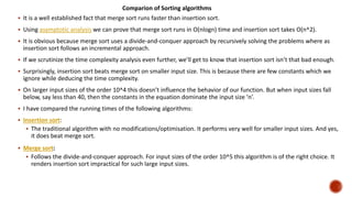
- 23. It is a well established fact that merge sort runs faster than insertion sort. Using asymptotic analysis we can prove that merge sort runs in O(nlogn) time and insertion sort takes O(n^2). It is obvious because merge sort uses a divide-and-conquer approach by recursively solving the problems where as insertion sort follows an incremental approach. If we scrutinize the time complexity analysis even further, we’ll get to know that insertion sort isn’t that bad enough. Surprisingly, insertion sort beats merge sort on smaller input size. This is because there are few constants which we ignore while deducing the time complexity. On larger input sizes of the order 10^4 this doesn’t influence the behavior of our function. But when input sizes fall below, say less than 40, then the constants in the equation dominate the input size ‘n’. I have compared the running times of the following algorithms: Insertion sort: The traditional algorithm with no modifications/optimisation. It performs very well for smaller input sizes. And yes, it does beat merge sort. Merge sort: Follows the divide-and-conquer approach. For input sizes of the order 10^5 this algorithm is of the right choice. It renders insertion sort impractical for such large input sizes. Comparion of Sorting algorithms
- 24. Combined version of insertion sort and merge sort: I have tweaked the logic of merge sort a little bit to achieve a considerably better running time for smaller input sizes. As we know, merge sort splits its input into two halves until it is trivial enough to sort the elements. But here, when the input size falls below a threshold such as ’n’ < 40 then this hybrid algorithm makes a call to traditional insertion sort procedure. From the fact that insertion sort runs faster on smaller inputs and merge sort runs faster on larger inputs, this algorithm makes best use both the worlds. Quick sort: I have not implemented this procedure. This is the library function qsort() which is available in . I have considered this algorithm in order to know the significance of implementation. It requires a great deal of programming expertise to minimize the number of steps and make at most use of the underlying language primitives to implement an algorithm in the best way possible. This is the main reason why it is recommended to use library functions. They are written to handle anything and everything. They optimize to the maximum extent possible. And before I forget, from my analysis qsort() runs blazingly fast on virtually any input size!