2. Table of contents
Introduction
Algorithm
Analysis of algorithms
Asymptotic Complexity
Asymptotic Notation
Conclusion
3. Introduction
• The methods of algorithm design form one of the
core practical technologies of computer science.
• The main aim of this lecture is to familiarize the
student with the framework used throughout the
course for the design and analysis of algorithms.
• The algorithms needed to solve computational
problems. The problem of sorting is used as a
running example.
• A pseudocode to show how we shall specify the
algorithms.
4. Algorithms
• The word algorithm comes from the name of a
Persian mathematician Abu Ja’far Mohammed ibn-
i Musa al Khowarizmi.
• In computer science, this word refers to a special
method useable by a computer for solution of a
problem.
• The statement of the problem specifies in general
terms the desired input/output relationship.
5. Algorithm
The word Algorithm means ” A set of finite rules or
instructions to be followed in calculations or other
problem-solving operations ”
Or
” A procedure for solving a mathematical problem in a
finite number of steps that frequently involves recursive
operations”.
7. Need for algorithms
1. Algorithms are necessary for solving complex
problems efficiently and effectively.
2. They help to automate processes and make them
more reliable, faster, and easier to perform.
3. Algorithms also enable computers to perform tasks
that would be difficult or impossible for humans to do
manually.
4. They are used in various fields such as mathematics,
computer science, engineering, finance, and many
others to optimize processes, analyze data, make
predictions, and provide solutions to problems.
8. Types of Algorithms:
1. Brute Force Algorithm:
It is the simplest approach to a problem. A brute force
algorithm is the first approach that comes to finding
when we see a problem.
2. Recursive Algorithm:
A recursive algorithm is based on recursion. In this case,
a problem is broken into several sub-parts and called
the same function again and again.
9. Cont…
3. Backtracking Algorithm:
The backtracking algorithm builds the solution by searching
among all possible solutions. Using this algorithm, we keep
on building the solution following criteria. Whenever a
solution fails we trace back to the failure point build on the
next solution and continue this process till we find the
solution or all possible solutions are looked after.
4. Searching Algorithm:
Searching algorithms are the ones that are used for
searching elements or groups of elements from a particular
data structure. They can be of different types based on
their approach or the data structure in which the element
should be found.
10. Cont…
5. Sorting Algorithm:
Sorting is arranging a group of data in a particular
manner according to the requirement. The algorithms
which help in performing this function are called sorting
algorithms. Generally sorting algorithms are used to sort
groups of data in an increasing or decreasing manner.
6. Hashing Algorithm:
Hashing algorithms work similarly to the searching
algorithm. But they contain an index with a key ID. In
hashing, a key is assigned to specific data.
11. Cont…
7. Divide and Conquer Algorithm:
This algorithm breaks a problem into sub-problems,
solves a single sub-problem, and merges the solutions to
get the final solution. It consists of the following three
steps: Divide, Solve, and Combine
8. Greedy Algorithm:
In this type of algorithm, the solution is built part by
part. The solution for the next part is built based on the
immediate benefit of the next part. The one solution
that gives the most benefit will be chosen as the
solution for the next part.
12. Cont…
9. Dynamic Programming Algorithm:
This algorithm uses the concept of using the already
found solution to avoid repetitive calculation of the
same part of the problem. It divides the problem into
smaller overlapping subproblems and solves them.
10. Randomized Algorithm:
In the randomized algorithm, we use a random number
so it gives immediate benefit. The random number
helps in deciding the expected outcome.
13. Analysis of algorithms
Why study algorithms and performance?
• Algorithms help us to understand scalability.
• Algorithmic mathematics provides a language for talking
about program behavior.
• Evaluate the performance of the algorithm based on the
given model and metrics: running time, and order of
growth.
•Kinds of analyses: Worst-case, Average-case, and Best-
case.
14. Asymptotic Complexity
Running time of an algorithm as a function of input size
n for large n.
Expressed using only the highest-order term in the
expression for the exact running time.
Describes behavior of function in the limit.
Written using Asymptotic Notation.
15. Asymptotic Notation
O, ,, o,
Defined for functions over the natural numbers.
Ex: f(n) = (n2
).
Describes how f(n) grows in comparison to n2
.
Define a set of functions; in practice used to
compare two function sizes.
The notations describe different rate-of-growth
relations between the defining function and the
defined set of functions.
16. O-notation
O(g(n)) = {f(n) :
positive constants c and n0,
such that n n0,
we have 0 f(n) cg(n) }
For function g(n), we define O(g(n)),
big-O of n, as the set:
g(n) is an asymptotic upper bound for f(n).
Intuitively: Set of all functions
whose rate of growth is the same as
or lower than that of g(n).
f(n) = O(g(n)).
17. Examples
Example: Find upper bound of running time of a linear
function f(n) = 6n + 3.
To find upper bound of f(n), we have to find c and
n0 such that 0 ≤ f (n) ≤ c × g (n) for all n ≥ n0
0 ≤ f (n) ≤ c × g (n)
0 ≤ 6n + 3 ≤ c × g (n)
0 ≤ 6n + 3 ≤ 6n + 3n, for all n ≥ 1 (There can be such
infinite possibilities)
0 ≤ 6n + 3 ≤ 9n
So, c = 9 and g (n) = n, n0 = 1
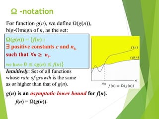
18. -notation
g(n) is an asymptotic lower bound for f(n).
Intuitively: Set of all functions
whose rate of growth is the same
as or higher than that of g(n).
f(n) = (g(n)).
(g(n)) = {f(n) :
positive constants c and n0,
such that n n0,
we have 0 cg(n) f(n)}
For function g(n), we define (g(n)),
big-Omega of n, as the set:
19. Examples
Example: Find lower bound of running time of a linear function
f(n) = 6n + 3.
To find lower bound of f(n), we have to find c and n0 such that 0
≤ c.g(n) ≤ f(n) for all n ≥ n0
0 ≤ c × g(n) ≤ f(n)
0 ≤ c × g(n) ≤ 6n + 3
0 ≤ 6n ≤ 6n + 3 → true, for all n ≥ n0
0 ≤ 5n ≤ 6n + 3 → true, for all n ≥ n0
Above both inequalities are true and there exists such infinite
inequalities. So,
f(n) = Ω (g(n)) = Ω (n) for c = 6, n0 = 1
f(n) = Ω (g(n)) = Ω (n) for c = 5, n0 = 1
and so on.
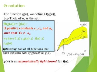
20. -notation
(g(n)) = {f(n) :
positive constants c1, c2, and n0,
such that n n0,
we have 0 c1g(n) f(n)
c2g(n)
}
For function g(n), we define (g(n)),
big-Theta of n, as the set:
g(n) is an asymptotically tight bound for f(n).
Intuitively: Set of all functions that
have the same rate of growth as g(n).
21. o-notation
f(n) becomes insignificant relative to g(n) as n
approaches infinity:
lim [f(n) / g(n)] = 0
n
g(n) is an upper bound for f(n) that is not
asymptotically tight.
o(g(n)) = {f(n): c > 0, n0 > 0 such that
n n0, we have 0 f(n) < cg(n)}.
For a given function g(n), the set little-o:
22. (g(n)) = {f(n): c > 0, n0 > 0 such that
n n0, we have 0 cg(n) < f(n)}.
-notation
f(n) becomes arbitrarily large relative to g(n) as n
approaches infinity:
lim [f(n) / g(n)] = .
n
g(n) is a lower bound for f(n) that is not asymptotically
tight.
For a given function g(n), the set little-omega:
23. Conclusion
To provide main notions of algorithm.
To learn formal framework to draw basic elements.
To study and analysis of algorithm along with
completeness.
To learn framework for application-based design.


![o-notation
f(n) becomes insignificant relative to g(n) as n
approaches infinity:
lim [f(n) / g(n)] = 0
n
g(n) is an upper bound for f(n) that is not
asymptotically tight.
o(g(n)) = {f(n): c > 0, n0 > 0 such that
n n0, we have 0 f(n) < cg(n)}.
For a given function g(n), the set little-o:](https://image.slidesharecdn.com/algorithms-1-250218164307-f0a8e8b2/85/analysis-of-algorithms-and-asymptotic-complexity-21-320.jpg)
![(g(n)) = {f(n): c > 0, n0 > 0 such that
n n0, we have 0 cg(n) < f(n)}.
-notation
f(n) becomes arbitrarily large relative to g(n) as n
approaches infinity:
lim [f(n) / g(n)] = .
n
g(n) is a lower bound for f(n) that is not asymptotically
tight.
For a given function g(n), the set little-omega:](https://image.slidesharecdn.com/algorithms-1-250218164307-f0a8e8b2/85/analysis-of-algorithms-and-asymptotic-complexity-22-320.jpg)