SlideShare a Scribd company logo
6
Most read
11
Most read
14
Most read
Artificial Intelligence-BCS515B
Dept. of CSE, CEC 2024-25
CITY ENGINEERING COLLEGE
Approved by AICTE New Delhi & Affiliated by VTU, Belagavi
Doddakallasandra, Off Kanakapura Main Road,
Next to Gokulam Apartment, Bangalore- 560 062.
Department of Computer Science and Engineering
COURSE NAME: ARTIFICIAL INTELLIGENCE
COURSE CODE: BCS515B
SEMESTER – V
Module 2
➢ 3.1 Problem‐solving:
Problem‐solving agents
➢ 3.2 Example problems
➢ 3.3 Searching for Solutions
➢ 3.4 Uninformed Search Strategies
➢ Chapter 3 - 3.1, 3.2, 3.3, 3.4
Reference:
Textbooks 1. Stuart J. Russell and Peter Norvig, Artificial Intelligence, 3rd
Edition, Pearson,2015.
Artificial Intelligence-BCS515B
Dept. of CSE, CEC 2024-25
Module 2
Problem-solving agent:
When the correct action to take is not immediately obvious, an agent may need to plan ahead:
to consider a sequence of actions that form a path to a goal state. Such an agent is called a
problem-solving agent, and the computational process it undertakes is called search.
Agents that use factored or structured representations of states are called planning agents.
3.1 PROBLEM-SOLVING AGENTS
• Reflex agents are too simple and have great difficulties in learning desired action
sequences
• Goal-based agents can succeed by considering Solving Problems by Searching Goal
future actions and the desirability of their outcomes.
• We now describe a special type of goal-based agents called problem-solving agents, which
try to find action sequences that lead to desirable states. These are uninformed algorithms;
they are given no hints or heuristics for the problem solution other than its definition.
• We first need a goal formulation, based on the current situation and the performance
measure.
• Problem formulation is the process of deciding what actions and states to consider, given
a goal.
• In general, an agent with several options for action of unknown value can decide what to
do by first examining different possible sequences of actions that lead to states of known
value, and then choosing the best sequence.
• For now we assume that the environment is observable and Discrete so at any given state
there are only finitely many actions to choose from. We will assume the environment is
known, so the agent knows which states are reached by each action. Finally, we assume
that the environment is deterministic, so each action has exactly one outcome.
The process of looking for a sequence of actions that reaches the goal is called search. A search
algorithm takes a problem as input and returns a solution in the form of an action sequence.
Once a solution is found, the actions it recommends can be carried out. This is called the
execution phase. Thus, we have a simple “formulate, search, execute” design for the agent, as
shown in Figure 3.1.
Notice that while the agent is executing the solution sequence it ignores its percepts when
choosing an action because it knows in advance what they will be. An agent that carries out its
plans with its eyes closed, so to speak, must be quite certain of what is going on. Control
theorists call this an open-loop system, because ignoring the percepts breaks the loop between
agent and environment.
Artificial Intelligence-BCS515B
Dept. of CSE, CEC 2024-25
Example Problem: Romania Tour
Imagine an agent enjoying a touring vacation in Romania. The agent wants to take in the sights,
improve its Romanian, enjoy the nightlife, avoid hangovers, and so on. The decision problem
is a complex one. Now, suppose the agent is currently in the city of Arad and has a
nonrefundable ticket to fly out of Bucharest the following day. The agent observes street signs
and sees that there are three roads leading out of Arad: one toward Sibiu, one to Timisoara, and
one to Zerind. None of these are the goal, so unless the agent is familiar with the geography of
Romania, it will not know which road to follow
Fig 3.2: A simplified road map of part of Romania.
Artificial Intelligence-BCS515B
Dept. of CSE, CEC 2024-25
we will assume our agents always have access to information about the world, such as the map
in Figure 3.2. With that information, the agent can follow this four-phase problem-solving
process:
• Goal formulation: The agent adopts the goal of reaching Bucharest. Goals organize
behavior by limiting the objectives and hence the actions to be considered.
• Problem formulation: The agent devises a description of the states and actions necessary
to reach the goal—an abstract model of the relevant part of the world. For our agent, one
good model is to consider the actions of traveling from one city to an adjacent city, and
therefore the only fact about the state of the world that will change due to an action is the
current city.
• Search : Before taking any action in the real world, the agent simulates sequences of actions
in its model, searching until it finds a sequence of actions that reaches the goal. Such a
sequence is called a solution. The agent might have to simulate multiple sequences that do
not reach the goal, but eventually it will find a solution (such as going from Arad to Sibiu
to Fagaras to Bucharest), or it will find that no solution is possible.
• Execution: The agent can now execute the actions in the solution, one at a time.
It is an important property that in a fully observable, deterministic, known environment, the
solution to any problem is a fixed sequence of actions: drive to Sibiu, then Fagaras, then
Bucharest. If the model is correct, then once the agent has found a solution, it can ignore its
percepts while it is executing the actions—closing its eyes, so to speak—because the solution is
guaranteed to lead to the goal. Control theorists call this an open-loop system: ignoring the
percepts breaks the loop between agent and environment. If there is a chance that the model is
incorrect, or the environment is nondeterministic, then the agent would be safer using a closed-
loop approach that monitors the precepts.
• Formulate goal:
• be in Bucharest
• Formulate problem:
• states: various cities
• actions: drive between cities
• Find solution:
• sequence of cities, e.g., Arad, Sibiu, Fagaras, Bucharest.
Single-State Problem Formulation
Artificial Intelligence-BCS515B
Dept. of CSE, CEC 2024-25
A description of the possible actions available to the agent. Given a particular state s,
ACTIONS(s) returns the set of actions that can be executed in s. We say that each of these
actions is applicable in s. For example, from the state In(Arad), the applicable actions are
{Go(Sibiu), Go(Timisoara), Go(Zerind)}.
A description of what each action does; the formal name for this is the transition model,
specified by a function RESULT(s, a) that returns the state that results from doing action a
in state s. We also use the term successor to refer to any state reachable from a given state
by a single action. For example, we have
RESULT(In(Arad),Go(Zerind)) = In(Zerind) .
A path cost function that assigns a numeric cost to each path. The step cost of taking action
a in state s to reach state s’ is denoted by c(s, a, s’).
Formulating problems:
Our formulation of the problem of getting to Bucharest is a model—an abstract mathematical
description—and not the real thing.
• Abstraction :The process of removing detail from a representation is called abstraction.
A good problem formulation has the right level of detail. If the actions were at the level
of “move the right foot forward a centimetre” or “turn the steering wheel one degree
left” the agent would probably never find its way out of the parking lot, let alone to
Bucharest.
• Level of abstraction: Think of the abstract states and actions we have chosen as
corresponding to large sets of detailed world states and detailed action sequences. Now
consider a solution to the abstract problem: for example, the path from Arad to Sibiu to
Rimnicu ,Vilcea to Pitesti to Bucharest. This abstract solution corresponds to a large
number of more detailed paths. For example, we could drive with the radio on between
Sibiu and Rimnicu Vilcea, and then switch it off for the rest of the trip.
• The abstraction is valid if we can elaborate any abstract solution into a solution in the
more detailed world; a sufficient condition is that for every detailed state that is “in
Arad,”there is a detailed path to some state that is “in Sibiu,” and so on.The
abstraction is useful if carrying out each of the actions in the solution is easier than the
original problem; in our case, the action “drive from Arad to Sibiu” can be carried
out without further search or planning by a driver with average skill.
Artificial Intelligence-BCS515B
Dept. of CSE, CEC 2024-25
3.2 EXAMPLE PROBLEMS
Astandardized problem is intended to illustrate or exercise various problem-solving methods.
It can be given a concise, exact description and hence is suitable as a benchmark for problem
researchers to compare the performance of algorithms. A real-world problem, such as robot
navigation, is one whose solutions people actually use, and whose formulation is idiosyncratic
not standardized, because, for example, each robot has different sensors that produce different
data.
Toy problems:
The first example we examine is the vacuum world.
A grid world problem is a two-dimensional rectangular array of square cells in which agents
can move from cell to cell. Typically, the agent can move to any obstacle-free adjacent cell—
horizontally or vertically and in some problems diagonally. Cells can contain objects, which
the agent can pick up, push, or otherwise act upon; a wall or other impassible obstacle in a cell
prevents an agent from moving into that cell. The vacuum world can be formulated as a grid
world problem as follows:
Figure 3.3 The state space for the vacuum world. Links denote actions: L = Left, R =Right, S = Suck.
• States: The state is determined by both the agent location and the dirt locations. The
agent is in one of two locations, each of which might or might not contain dirt. Thus,
there are 2 × 22
= 8 possible world states. A larger environment with n locations has
n x 2n states.
• Initial state: Any state can be designated as the initial state.
• Actions: In this simple environment, each state has just three actions: Left, Right, and
Suck. Larger environments might also include Up and Down.
• Transition model: The actions have their expected effects, except that moving Left in
the leftmost square, moving Right in the rightmost square, and Sucking in a clean square
have no effect. The complete state space is shown in Figure 3.3.
• Goal test: This checks whether all the squares are clean.
• Path cost: Each step costs 1, so the path cost is the number of steps in the path.
Artificial Intelligence-BCS515B
Dept. of CSE, CEC 2024-25
8-Puzzle:
The 8-puzzle, an instance of which is shown in Figure 3.3, consists of a 3×3 board with eight
numbered tiles and a blank space. A tile adjacent to the blank space can slide into the space.
The object is to reach a specified goal state, such as the one shown on the right of the figure.
The standard formulation is as follows:
Figure 3.4 A typical instance of the 8-puzzle.
The 8-puzzle belongs to the family of sliding-block puzzles, which are often used as test
problems for new search algorithms in AI. This family is known to be NP-complete, so one
does not expect to find methods significantly better in the worst case than the search algorithms
described in this chapter and the next. The 8-puzzle has 9!/2=181, 440 reachable states and is
easily solved. The 15-puzzle (on a 4×4 board) has around 1.3 trillion states, and random
instances can be solved optimally in a few milliseconds by the best search algorithms. The 24-
puzzle (on a 5 × 5 board) has around 1025 states, and random instances take several hours to
solve optimally.
8-Queens Problem:
The goal of the 8-queens problem is to place eight queens on a chessboard such that no queen
attacks any other. There are two main kinds of formulation. An incremental formulation
involves operators that augment the state description, starting with an empty state; for the 8-
queens problem, this means that each action adds a queen to the state. A complete-state
formulation starts with all 8 queens on the board and moves them around. In either case, the
path cost is of no interest because only the final state counts. The first incremental formulation
one might try is the following:
• States: Any arrangement of 0 to 8 queens on the board is a state.
• Initial state: No queens on the board.
• Actions: Add a queen to any empty square.
• Transition model: Returns the board with a queen added to the specified square.
• Goal test: 8 queens are on the board, none attacked.
Artificial Intelligence-BCS515B
Dept. of CSE, CEC 2024-25
In this formulation, we have 64 ・ 63 ・ ・ ・ 57 ≈ 1.8×10¹⁴ possible sequences to
investigate. A better formulation would prohibit placing a queen in any square that is already
attacked:
• States: All possible arrangements of n queens (0 ≤ n ≤ 8), one per column in the leftmost n
columns, with no queen attacking another.
• Actions: Add a queen to any square in the leftmost empty column such that it is not attacked
by any other queen.
This formulation reduces the 8-queens state space from 1.8×10¹⁴ to just 2,057, and solutions
are easy to find. Our final toy problem was devised by Donald Knuth (1964) and illustrates
how infinite state spaces can arise. Knuth conjectured that, starting with the number 4, a
sequence of factorial, square root, and floor operations will reach any desired positive integer.
For example, we can reach 5 from 4 as follows:
The problem definition is very simple:
• States: Positive numbers.
• Initial state: 4.
• Actions: Apply factorial, square root, or floor operation (factorial for integers only).
• Transition model: As given by the mathematical definitions of the operations.
• Goal test: State is the desired positive integer.
Real-world problems
1) Airline travel problems:
States: Each state obviously includes a location (e.g., an airport) and the current time
Furthermore, because the cost of an action (a flight segment) may depend on previous
segments, their fare bases, and their status as domestic or international, the state must
record extra information about these “historical” aspects.
Artificial Intelligence-BCS515B
Dept. of CSE, CEC 2024-25
• Initial state: This is specified by the user’s query.
• Actions: Take any flight from the current location, in any seat class, leaving after the current
time, leaving enough time for within-airport transfer if needed.
• Transition model: The state resulting from taking a flight will have the flight’s destination
as the current location and the flight’s arrival time as the current time.
• Goal test: Are we at the final destination specified by the user?
• Path cost: This depends on monetary cost, waiting time, flight time, customs and immigration
procedures, seat quality, time of day, type of airplane, frequent-flyer mileage awards, and so
on.
2) Route-finding problems
3) GPS-based navigation systems,
Google maps
4) Touring problems
5) Real-World Search Problems
6) TSP (traveling salesperson problem)
7) VLSI layout problems
8) Robot navigation problems
9) Automatic assembly sequencing
10) Internet searching
11) Searching paths in metabolic
networks in
12) Bioinformatics
13) protein design
3.3 SEARCHING FOR SOLUTIONS:
Asolution is an action sequence, so search algorithms work by considering various possible action
sequences. The possible action sequences starting at the initial state form a search tree with the
initial state at the root; the branches are actions and the nodes correspond to states in the state
space of the problem. Figure 3.6 shows the first few steps in growing the search tree for finding a
route from Arad to Bucharest.
The root node of the tree corresponds to the initial state, In(Arad).The first step is to test whether
this is a goal state. (Clearly it is not, but it is important to check so that we can solve trick problems
like “starting in Arad, get to Arad.”) Then we need to consider taking various actions. We do this
by expanding the current state; that is, applying each legal action to the current state, thereby
generating a new set of states. In this case, we add three branches from the parent node In(Arad)
leading to three new child nodes: In(Sibiu), In(Timisoara), and In(Zerind).
We check to see whether it is a goal state (it is not) and then expand it to get In(Arad), In(Fagaras),
In(Oradea), and In(RimnicuVilcea). We can then choose any of these four or go back and choose
Timisoara or Zerind. Each of these six nodes is a leaf node, that is, a node with no children in the
tree. The set of all leaf nodes available for expansion at any given point is called the frontier.
(Many authors call it the open list, which is both geographically less evocative and less accurate,
because other data structures are better suited than a list.)
Artificial Intelligence-BCS515B
Dept. of CSE, CEC 2024-25
Artificial Intelligence-BCS515B
Dept. of CSE, CEC 2024-25
As the saying goes, algorithms that forget their history are doomed to repeat it. The way to avoid
exploring redundant paths is to remember where one has been .To do this, we augment the
algorithm with a data structure called the explored set (also known as the closed list), which
remembers every expanded node. Newly generated nodes that match previously generated
nodes—ones in the explored set or the frontier—can be discarded instead of being added to the
frontier. The new algorithm, called GRAPH-SEARCH, is shown informally in Figure 3.7. The
specific algorithms in this chapter draw on this general design.
3.3.1 Infrastructure for search algorithms
Search algorithms require a data structure to keep track of the search tree that is being constructed.
For each node n of the tree, we have a structure that contains four components:
• n.STATE: the state in the state space to which the node corresponds;
• n.PARENT: the node in the search tree that generated this node;
• n.ACTION: the action that was applied to the parent to generate the node;
Artificial Intelligence-BCS515B
Dept. of CSE, CEC 2024-25
• n.PATH-COST: the cost, traditionally denoted by g(n), of the path from the initial state to the
node, as indicated by the parent pointers.
The node data structure is depicted in Figure 3.10. Notice how the PARENT pointer string the
nodes together into a tree structure. These pointers also allow the solution path to be extracted
when a goal node is found; we use the SOLUTION function to return the sequence of actions
obtained by following parent pointers back to the root.
The appropriate data structure for this is a queue. The operations on a queue are as follows:
• EMPTY?(queue) returns true only if there are no more elements in the queue.
• POP(queue) removes the first element of the queue and returns it.
• INSERT(element, queue) inserts an element and returns the resulting queue.
Queues are characterized by the order in which they store the inserted nodes. Three common
variants are the first-in, first-out or FIFO queue, which pops the oldest element of the queue;the
last-in, first-out or LIFO queue (also known as a stack), which pops the newest element of the
queue; and the priority queue, which pops the element of the queue with the highest
priority according to some ordering function.
3.3.2 Measuring problem-solving performance
We can evaluate an algorithm’s performance in four ways:
• Completeness: Is the algorithm guaranteed to find a solution when there is one?
• Optimality: Does the strategy find the optimal solution, as defined on page 68?
• Time complexity: How long does it take to find a solution?
• Space complexity: How much memory is needed to perform the search?
Artificial Intelligence-BCS515B
Dept. of CSE, CEC 2024-25
Complexity is expressed in terms of three quantities:
b, the branching factor or maximum number of successors of any node;
d, the depth of the shallowest goal node (i.e., the number of steps along the path from
the root); and m, the maximum length of any path in the state space.
m: maximum depth of the state space (may be ∞).
To assess the effectiveness of a search algorithm, we can consider just the search cost—which
typically depends on the time complexity but can also include a term for memory usage—or we
can use the total cost, which combines the search cost and the path cost of the solution found.
3.4 UNINFORMED SEARCH STRATEGIES
The Uninformed Search term means that the strategies have no additional information about states
beyond that provided in the problem definition. All they can do is generate successors and
distinguish a goal state from a non-goal state. All search strategies are distinguished by the order
in which nodes are expanded. Strategies that know whether one non-goal state is “more
promising” than another are called informed search or heuristic search strategies.
• Breadth-first search (BFS)
• Uniform-cost search
• Depth-first search (DFS)
• Depth-limited search
• Iterative deepening search
• Bidirectional Search
3.4.1 Breadth-first search
• The root node is expanded first
• Then all successors of the root node are expanded
• Then all their successors and so on
• In general, all the nodes of a given depth are expanded
• before any node of the next depth is expanded.
• Uses a standard queue as data structure.
Pseudocode is given in Figure 3.11. Figure 3.12 shows the progress of the search on a simple
binary tree.
Imagine searching a uniform tree where every state has b successors. The root of the search tree
generates b nodes at the first level, each of which generates b more nodes, for a total of b2
at the
second level. Each of these generates b more nodes, yielding b3
nodes at the third level, and so on.
Now suppose that the solution is at depth d. In the worst case, it is the last node generated at that
level. Then the total number of nodes generated is
Artificial Intelligence-BCS515B
Dept. of CSE, CEC 2024-25
Two lessons can be learned from Figure 3.13.
First, the memory requirements are a bigger problem for breadth-first search than is the execution
time. One might wait 13 days for the solution to an important problem with search depth 12, but
no personal computer has the petabyte of memory it would take. Fortunately, other strategies
require less memory.
The second lesson is that time is still a major factor. If your problem has a solution at depth 16,
then (given our assumptions) it will take about 350 years for breadth-first search (or indeed any
uninformed search) to find it. In general, exponential-complexity search problems cannot be
solved by uninformed methods for any but the smallest instances.
Artificial Intelligence-BCS515B
Dept. of CSE, CEC 2024-25
3.4.2 Uniform-cost search
• Modification to BFS generates Uniform-cost search, which works with any step-cost
function ( edge weights/costs):
• UCS expands the node n with lowest summed path cost g(n).
• To do this, the frontier is stored as a priority queue. (Sorted list data structure, better heap
data structure).
• The goal test is applied to a node when selected for expansion (not when it is generated).
• Also a test is added if a better node is found to a node on the frontier.
The algorithm is shown in Figure 3.14.
Artificial Intelligence-BCS515B
Dept. of CSE, CEC 2024-25
The Modifications come into play in the example shown in Figure 3.15, where the problem is
to get from Sibiu to Bucharest. The Uniform Search is similar to Dijkstra’s algorithm. It
requires that all step costs are non-negative. It may get stuck if there is a path with an infinite
sequence of zero cost steps. Otherwise it is complete.
3.4.3 Depth-first search
• DFS alwas expands the deepest node in the current frontier of the search tree.
• It uses a stack (LIFO queue last in first out)
• DFS is frequently programmed recursively, then the program call stack is the LIFO
queue.
• DFS is complete, if the graph is finite.
• The tree search version of DFS is complete on a finite tree, if a test is included
whether the node has already been visited
• DFS is incomplete on infinite trees or graphs.
• DFS has time complexity O(bm
), if m is the maximum depth of any node (may be
infinite).
• DFS has space complexity of O(b m)
• As an alternative to the GRAPH-SEARCH-style implementation, it is common to
implement depth-first search with a recursive function that calls itself on each of its
children in turn.
In Figure 3.16, depth first search will explore the entire left subtree even if node C is a goal
node. If node J were also a goal node, then depth-first search would return it as a solution
instead of C, which would be a better solution; hence, depth-first search is not optimal.
The time complexity of depth-first graph search is bounded by the size of the state space (which
may be infinite, of course). A depth-first tree search, on the other hand, may generate all of the
O(bm) nodes in the search tree, where m is the maximum depth of any node; this can be much
greater than the size of the state space. Note that m itself can be much larger than d (the depth
of the shallowest solution) and is infinite if the tree is unbounded.
A variant of depth-first search called backtracking search uses still less memory. In
backtracking, only one successor is generated at a time rather than all successors; each partially
expanded node remembers which successor to generate next. In this way, only O(m) memory
is needed rather than O(bm). Backtracking search facilitates yet another memory-saving (and
time-saving) trick: the idea of generating a successor by modifying the current state description
directly rather than copying it first. This reduces the memory requirements to just one state
description and O(m) actions.
Artificial Intelligence-BCS515B
Dept. of CSE, CEC 2024-25
3.4.4 Depth-limited search
• The failure of DFS in infinite search spaces can be prevented by giving it a search
limit l .This approach is called depth limited search
• Unfortunately, it is not complete if we choose l < d, where d is the depth of the goal
node.
• This happens easily, because d is unknown.
• Depth-limited search has time complexity O(b l).
• It has space complexity of O(b l).
• However, in some applications we know a depth limit (# nodes in a graph, maximum
diameter, …)
• Depth-first search can be viewed as a special case of depth-limited search with l =∞.
Artificial Intelligence-BCS515B
Dept. of CSE, CEC 2024-25
3.4.5 Iterative deepening depth-first search
The iterative deepening search algorithm repeatedly applies depth-limited search with
increasing limits. It terminates when a solution is found or if the depth limited
search returns failure, meaning that no solution exists. This search is also frequently called
depth-first iterative deepening (DFID).
Iterative deepening search (or iterative deepening depth-first search) is a general strategy,
often used in combination with depth-first tree search, that finds the best depth limit. It does
this by gradually increasing the limit—first 0, then 1, then 2, and so on—until a goal is found.
This will occur when the depth limit reaches d, the depth of the shallowest goal node. The
algorithm is shown in Figure 3.18. Iterative deepening combines the benefits of depth-first and
breadth-first search. Like depth-first search, its memory requirements are modest: O(bd) to be
precise. Like breadth-first search, it is complete when the branching factor is finite and optimal
when the path cost is a nondecreasing function of the depth of the node. Figure 3.19 shows four
iterations of on a binary search tree, where the solution is found on the fourth iteration.
Artificial Intelligence-BCS515B
Dept. of CSE, CEC 2024-25
The total number of nodes generated in the worst case is
3.4.6 Bidirectional search
The idea behind bidirectional search is to run two simultaneous searches—one forward
from the initial state and the other backward from the goal—hoping that the two
searches meet in the middle (Figure 3.20). The motivation is that bd/2
+ bd/2
is much less
than bd
, or in the figure, the area of the two small circles is less than the area of one big
circle centered on the start and reaching to the goal.
The time complexity of bidirectional search using breadth-first searches in both
directions is O(bd/2
). The space complexity is also O(bd/2
). We can reduce this by
roughly half if one of the two searches is done by iterative deepening, but at least one
Artificial Intelligence-BCS515B
Dept. of CSE, CEC 2024-25
of the frontiers must be kept in memory so that the intersection check can be done. This
space requirement is the most significant weakness of bidirectional search.
Advantage:
delays exponential growth by reducing the exponent for time and space
complexity in half.
Disadvantage:
At every time point the two fringes must be compared. This requires an
efficient hashing data structure
Bidirectional search also requires to search backward (predecessors of a state).
This is not always possible.
3.4.7 Comparing uninformed search strategies
Figure 3.21 compares search strategies in terms of the four evaluation criteria set forth in
Section 3.3.2. This comparison is for tree-search versions. For graph searches, the main
differences are that depth-first search is complete for finite state spaces and that the space and
time complexities are bounded by the size of the state space.

More Related Content

What's hot (10)

PPTX
Cognitive radio networks
sangitaholkar
 
PPTX
AI3391 Session 12 Local search in continious space.pptx
Guru Nanak Technical Institutions
 
PPTX
An Introduction to Soft Computing
Tameem Ahmad
 
PPTX
Artificial intelligence
Vikram Kumar
 
PDF
AI Lesson 03
Assistant Professor
 
PDF
Neural Networks: Support Vector machines
Mostafa G. M. Mostafa
 
DOCX
Artificial Intelligence
Akshay Thakur
 
PPTX
Jarrar: Description Logic
Mustafa Jarrar
 
PPTX
Unit 1 Fundamentals of Artificial Intelligence-Part I.pptx
DrYogeshDeshmukh1
 
PDF
First Order Logic resolution
Amar Jukuntla
 
Cognitive radio networks
sangitaholkar
 
AI3391 Session 12 Local search in continious space.pptx
Guru Nanak Technical Institutions
 
An Introduction to Soft Computing
Tameem Ahmad
 
Artificial intelligence
Vikram Kumar
 
AI Lesson 03
Assistant Professor
 
Neural Networks: Support Vector machines
Mostafa G. M. Mostafa
 
Artificial Intelligence
Akshay Thakur
 
Jarrar: Description Logic
Mustafa Jarrar
 
Unit 1 Fundamentals of Artificial Intelligence-Part I.pptx
DrYogeshDeshmukh1
 
First Order Logic resolution
Amar Jukuntla
 

Similar to BCS515B Module1 vtu notes : Artificial Intelligence Module 2.pdf (20)

PDF
Week 4.pdf
ZamshedForman1
 
PDF
ai-module-2-ppArtificial Intelligentt.pdf
ShylaBg1
 
PPTX
Problem Solving Agents-Introduction_L3.pptx
321910303040gitam
 
PDF
3 SOLVING PROBLEMS BY SEARCHING
Jim Webb
 
PPT
3.AILec5nkjnkjnkjnkjnkjnjhuhgvkjhbkhj-6.ppt
ShakibHasan53
 
PDF
AI Chapter Two Solving problems by searching.pdf
yeabtse1234
 
PPTX
3. Module_2_Chapter_3hvghcyttrctrctfcf.pptx
gkavitha5225
 
PPTX
Artificial intelligence(04)
Nazir Ahmed
 
PPTX
chapterThree.pptx
chalachew5
 
PPT
Articial intelligence chapter 3 problem solver.ppt
gadisaAdamu
 
PPTX
Module 2.pptx...........................
ssuserd60896
 
PDF
Lecture is related to the topic of Artificial intelligence
mohsinwaseer1
 
PDF
Artificial Intelegince-chapter three-problem solving.pdf
nooreldeenmagdy2
 
PPT
3 probsolver edited.ppt
HenokGetachew15
 
PPT
22sch AI Module 2.ppt 22sch AI Module 2.ppt
BHAVANABIDARKAR
 
PPT
22sch AI Module 2.ppt 22sch AI Module 2.ppt
BHAVANABIDARKAR
 
PPTX
CS 3491 Artificial Intelligence and Machine Learning Unit I Problem Solving
BalamuruganV28
 
PPTX
Problem solving in Artificial Intelligence.pptx
kitsenthilkumarcse
 
PDF
problem solving in Artificial intelligence .pdf
ElectricalTech3
 
PDF
AI 03 Solving Problems By Searching
Justin Knight
 
Week 4.pdf
ZamshedForman1
 
ai-module-2-ppArtificial Intelligentt.pdf
ShylaBg1
 
Problem Solving Agents-Introduction_L3.pptx
321910303040gitam
 
3 SOLVING PROBLEMS BY SEARCHING
Jim Webb
 
3.AILec5nkjnkjnkjnkjnkjnjhuhgvkjhbkhj-6.ppt
ShakibHasan53
 
AI Chapter Two Solving problems by searching.pdf
yeabtse1234
 
3. Module_2_Chapter_3hvghcyttrctrctfcf.pptx
gkavitha5225
 
Artificial intelligence(04)
Nazir Ahmed
 
chapterThree.pptx
chalachew5
 
Articial intelligence chapter 3 problem solver.ppt
gadisaAdamu
 
Module 2.pptx...........................
ssuserd60896
 
Lecture is related to the topic of Artificial intelligence
mohsinwaseer1
 
Artificial Intelegince-chapter three-problem solving.pdf
nooreldeenmagdy2
 
3 probsolver edited.ppt
HenokGetachew15
 
22sch AI Module 2.ppt 22sch AI Module 2.ppt
BHAVANABIDARKAR
 
22sch AI Module 2.ppt 22sch AI Module 2.ppt
BHAVANABIDARKAR
 
CS 3491 Artificial Intelligence and Machine Learning Unit I Problem Solving
BalamuruganV28
 
Problem solving in Artificial Intelligence.pptx
kitsenthilkumarcse
 
problem solving in Artificial intelligence .pdf
ElectricalTech3
 
AI 03 Solving Problems By Searching
Justin Knight
 
Ad

More from Swetha A (12)

PPTX
Microcontroller(18CS44) module 1
Swetha A
 
PPT
MISSION TO PLANETS (CHANDRAYAAN,MAVEN,CURIOSITY,MANGALYAAN,CASSINI SOLSTICE M...
Swetha A
 
PPTX
Few Indicies(NDVI... etc) performed on ERDAS software using Model Maker
Swetha A
 
PPTX
Steps for Principal Component Analysis (pca) using ERDAS software
Swetha A
 
PPTX
Digitising using ERDAS software
Swetha A
 
PPT
Map to Image Georeferencing using ERDAS software
Swetha A
 
PPTX
Developing Efficient Web-based GIS Applications
Swetha A
 
DOCX
GIS software
Swetha A
 
PPTX
GEOPROCESSING IN QGIS
Swetha A
 
PPT
Glacier and snow
Swetha A
 
PPT
Remote Sensing And GIS Application In Mineral , Oil , Ground Water MappingMin...
Swetha A
 
PPT
Remote Sensing And GIS Application In Wetland Mapping
Swetha A
 
Microcontroller(18CS44) module 1
Swetha A
 
MISSION TO PLANETS (CHANDRAYAAN,MAVEN,CURIOSITY,MANGALYAAN,CASSINI SOLSTICE M...
Swetha A
 
Few Indicies(NDVI... etc) performed on ERDAS software using Model Maker
Swetha A
 
Steps for Principal Component Analysis (pca) using ERDAS software
Swetha A
 
Digitising using ERDAS software
Swetha A
 
Map to Image Georeferencing using ERDAS software
Swetha A
 
Developing Efficient Web-based GIS Applications
Swetha A
 
GIS software
Swetha A
 
GEOPROCESSING IN QGIS
Swetha A
 
Glacier and snow
Swetha A
 
Remote Sensing And GIS Application In Mineral , Oil , Ground Water MappingMin...
Swetha A
 
Remote Sensing And GIS Application In Wetland Mapping
Swetha A
 
Ad

Recently uploaded (20)

PPTX
Continental Accounting in Odoo 18 - Odoo Slides
Celine George
 
PPTX
Introduction to Probability(basic) .pptx
purohitanuj034
 
PPTX
Basics and rules of probability with real-life uses
ravatkaran694
 
PPTX
K-Circle-Weekly-Quiz12121212-May2025.pptx
Pankaj Rodey
 
PPTX
Cybersecurity: How to Protect your Digital World from Hackers
vaidikpanda4
 
PDF
TOP 10 AI TOOLS YOU MUST LEARN TO SURVIVE IN 2025 AND ABOVE
digilearnings.com
 
DOCX
pgdei-UNIT -V Neurological Disorders & developmental disabilities
JELLA VISHNU DURGA PRASAD
 
PPTX
Electrophysiology_of_Heart. Electrophysiology studies in Cardiovascular syste...
Rajshri Ghogare
 
PPTX
PROTIEN ENERGY MALNUTRITION: NURSING MANAGEMENT.pptx
PRADEEP ABOTHU
 
PPTX
TOP 10 AI TOOLS YOU MUST LEARN TO SURVIVE IN 2025 AND ABOVE
digilearnings.com
 
PPTX
YSPH VMOC Special Report - Measles Outbreak Southwest US 7-20-2025.pptx
Yale School of Public Health - The Virtual Medical Operations Center (VMOC)
 
PDF
BÀI TẬP TEST BỔ TRỢ THEO TỪNG CHỦ ĐỀ CỦA TỪNG UNIT KÈM BÀI TẬP NGHE - TIẾNG A...
Nguyen Thanh Tu Collection
 
PPTX
CONCEPT OF CHILD CARE. pptx
AneetaSharma15
 
PDF
EXCRETION-STRUCTURE OF NEPHRON,URINE FORMATION
raviralanaresh2
 
PPTX
ENGLISH 8 WEEK 3 Q1 - Analyzing the linguistic, historical, andor biographica...
OliverOllet
 
PDF
The-Invisible-Living-World-Beyond-Our-Naked-Eye chapter 2.pdf/8th science cur...
Sandeep Swamy
 
PPT
DRUGS USED IN THERAPY OF SHOCK, Shock Therapy, Treatment or management of shock
Rajshri Ghogare
 
PPTX
Introduction to pediatric nursing in 5th Sem..pptx
AneetaSharma15
 
PPTX
Applications of matrices In Real Life_20250724_091307_0000.pptx
gehlotkrish03
 
PPTX
HEALTH CARE DELIVERY SYSTEM - UNIT 2 - GNM 3RD YEAR.pptx
Priyanshu Anand
 
Continental Accounting in Odoo 18 - Odoo Slides
Celine George
 
Introduction to Probability(basic) .pptx
purohitanuj034
 
Basics and rules of probability with real-life uses
ravatkaran694
 
K-Circle-Weekly-Quiz12121212-May2025.pptx
Pankaj Rodey
 
Cybersecurity: How to Protect your Digital World from Hackers
vaidikpanda4
 
TOP 10 AI TOOLS YOU MUST LEARN TO SURVIVE IN 2025 AND ABOVE
digilearnings.com
 
pgdei-UNIT -V Neurological Disorders & developmental disabilities
JELLA VISHNU DURGA PRASAD
 
Electrophysiology_of_Heart. Electrophysiology studies in Cardiovascular syste...
Rajshri Ghogare
 
PROTIEN ENERGY MALNUTRITION: NURSING MANAGEMENT.pptx
PRADEEP ABOTHU
 
TOP 10 AI TOOLS YOU MUST LEARN TO SURVIVE IN 2025 AND ABOVE
digilearnings.com
 
YSPH VMOC Special Report - Measles Outbreak Southwest US 7-20-2025.pptx
Yale School of Public Health - The Virtual Medical Operations Center (VMOC)
 
BÀI TẬP TEST BỔ TRỢ THEO TỪNG CHỦ ĐỀ CỦA TỪNG UNIT KÈM BÀI TẬP NGHE - TIẾNG A...
Nguyen Thanh Tu Collection
 
CONCEPT OF CHILD CARE. pptx
AneetaSharma15
 
EXCRETION-STRUCTURE OF NEPHRON,URINE FORMATION
raviralanaresh2
 
ENGLISH 8 WEEK 3 Q1 - Analyzing the linguistic, historical, andor biographica...
OliverOllet
 
The-Invisible-Living-World-Beyond-Our-Naked-Eye chapter 2.pdf/8th science cur...
Sandeep Swamy
 
DRUGS USED IN THERAPY OF SHOCK, Shock Therapy, Treatment or management of shock
Rajshri Ghogare
 
Introduction to pediatric nursing in 5th Sem..pptx
AneetaSharma15
 
Applications of matrices In Real Life_20250724_091307_0000.pptx
gehlotkrish03
 
HEALTH CARE DELIVERY SYSTEM - UNIT 2 - GNM 3RD YEAR.pptx
Priyanshu Anand
 

BCS515B Module1 vtu notes : Artificial Intelligence Module 2.pdf

  • 1. Artificial Intelligence-BCS515B Dept. of CSE, CEC 2024-25 CITY ENGINEERING COLLEGE Approved by AICTE New Delhi & Affiliated by VTU, Belagavi Doddakallasandra, Off Kanakapura Main Road, Next to Gokulam Apartment, Bangalore- 560 062. Department of Computer Science and Engineering COURSE NAME: ARTIFICIAL INTELLIGENCE COURSE CODE: BCS515B SEMESTER – V Module 2 ➢ 3.1 Problem‐solving: Problem‐solving agents ➢ 3.2 Example problems ➢ 3.3 Searching for Solutions ➢ 3.4 Uninformed Search Strategies ➢ Chapter 3 - 3.1, 3.2, 3.3, 3.4 Reference: Textbooks 1. Stuart J. Russell and Peter Norvig, Artificial Intelligence, 3rd Edition, Pearson,2015.
  • 2. Artificial Intelligence-BCS515B Dept. of CSE, CEC 2024-25 Module 2 Problem-solving agent: When the correct action to take is not immediately obvious, an agent may need to plan ahead: to consider a sequence of actions that form a path to a goal state. Such an agent is called a problem-solving agent, and the computational process it undertakes is called search. Agents that use factored or structured representations of states are called planning agents. 3.1 PROBLEM-SOLVING AGENTS • Reflex agents are too simple and have great difficulties in learning desired action sequences • Goal-based agents can succeed by considering Solving Problems by Searching Goal future actions and the desirability of their outcomes. • We now describe a special type of goal-based agents called problem-solving agents, which try to find action sequences that lead to desirable states. These are uninformed algorithms; they are given no hints or heuristics for the problem solution other than its definition. • We first need a goal formulation, based on the current situation and the performance measure. • Problem formulation is the process of deciding what actions and states to consider, given a goal. • In general, an agent with several options for action of unknown value can decide what to do by first examining different possible sequences of actions that lead to states of known value, and then choosing the best sequence. • For now we assume that the environment is observable and Discrete so at any given state there are only finitely many actions to choose from. We will assume the environment is known, so the agent knows which states are reached by each action. Finally, we assume that the environment is deterministic, so each action has exactly one outcome. The process of looking for a sequence of actions that reaches the goal is called search. A search algorithm takes a problem as input and returns a solution in the form of an action sequence. Once a solution is found, the actions it recommends can be carried out. This is called the execution phase. Thus, we have a simple “formulate, search, execute” design for the agent, as shown in Figure 3.1. Notice that while the agent is executing the solution sequence it ignores its percepts when choosing an action because it knows in advance what they will be. An agent that carries out its plans with its eyes closed, so to speak, must be quite certain of what is going on. Control theorists call this an open-loop system, because ignoring the percepts breaks the loop between agent and environment.
  • 3. Artificial Intelligence-BCS515B Dept. of CSE, CEC 2024-25 Example Problem: Romania Tour Imagine an agent enjoying a touring vacation in Romania. The agent wants to take in the sights, improve its Romanian, enjoy the nightlife, avoid hangovers, and so on. The decision problem is a complex one. Now, suppose the agent is currently in the city of Arad and has a nonrefundable ticket to fly out of Bucharest the following day. The agent observes street signs and sees that there are three roads leading out of Arad: one toward Sibiu, one to Timisoara, and one to Zerind. None of these are the goal, so unless the agent is familiar with the geography of Romania, it will not know which road to follow Fig 3.2: A simplified road map of part of Romania.
  • 4. Artificial Intelligence-BCS515B Dept. of CSE, CEC 2024-25 we will assume our agents always have access to information about the world, such as the map in Figure 3.2. With that information, the agent can follow this four-phase problem-solving process: • Goal formulation: The agent adopts the goal of reaching Bucharest. Goals organize behavior by limiting the objectives and hence the actions to be considered. • Problem formulation: The agent devises a description of the states and actions necessary to reach the goal—an abstract model of the relevant part of the world. For our agent, one good model is to consider the actions of traveling from one city to an adjacent city, and therefore the only fact about the state of the world that will change due to an action is the current city. • Search : Before taking any action in the real world, the agent simulates sequences of actions in its model, searching until it finds a sequence of actions that reaches the goal. Such a sequence is called a solution. The agent might have to simulate multiple sequences that do not reach the goal, but eventually it will find a solution (such as going from Arad to Sibiu to Fagaras to Bucharest), or it will find that no solution is possible. • Execution: The agent can now execute the actions in the solution, one at a time. It is an important property that in a fully observable, deterministic, known environment, the solution to any problem is a fixed sequence of actions: drive to Sibiu, then Fagaras, then Bucharest. If the model is correct, then once the agent has found a solution, it can ignore its percepts while it is executing the actions—closing its eyes, so to speak—because the solution is guaranteed to lead to the goal. Control theorists call this an open-loop system: ignoring the percepts breaks the loop between agent and environment. If there is a chance that the model is incorrect, or the environment is nondeterministic, then the agent would be safer using a closed- loop approach that monitors the precepts. • Formulate goal: • be in Bucharest • Formulate problem: • states: various cities • actions: drive between cities • Find solution: • sequence of cities, e.g., Arad, Sibiu, Fagaras, Bucharest. Single-State Problem Formulation
  • 5. Artificial Intelligence-BCS515B Dept. of CSE, CEC 2024-25 A description of the possible actions available to the agent. Given a particular state s, ACTIONS(s) returns the set of actions that can be executed in s. We say that each of these actions is applicable in s. For example, from the state In(Arad), the applicable actions are {Go(Sibiu), Go(Timisoara), Go(Zerind)}. A description of what each action does; the formal name for this is the transition model, specified by a function RESULT(s, a) that returns the state that results from doing action a in state s. We also use the term successor to refer to any state reachable from a given state by a single action. For example, we have RESULT(In(Arad),Go(Zerind)) = In(Zerind) . A path cost function that assigns a numeric cost to each path. The step cost of taking action a in state s to reach state s’ is denoted by c(s, a, s’). Formulating problems: Our formulation of the problem of getting to Bucharest is a model—an abstract mathematical description—and not the real thing. • Abstraction :The process of removing detail from a representation is called abstraction. A good problem formulation has the right level of detail. If the actions were at the level of “move the right foot forward a centimetre” or “turn the steering wheel one degree left” the agent would probably never find its way out of the parking lot, let alone to Bucharest. • Level of abstraction: Think of the abstract states and actions we have chosen as corresponding to large sets of detailed world states and detailed action sequences. Now consider a solution to the abstract problem: for example, the path from Arad to Sibiu to Rimnicu ,Vilcea to Pitesti to Bucharest. This abstract solution corresponds to a large number of more detailed paths. For example, we could drive with the radio on between Sibiu and Rimnicu Vilcea, and then switch it off for the rest of the trip. • The abstraction is valid if we can elaborate any abstract solution into a solution in the more detailed world; a sufficient condition is that for every detailed state that is “in Arad,”there is a detailed path to some state that is “in Sibiu,” and so on.The abstraction is useful if carrying out each of the actions in the solution is easier than the original problem; in our case, the action “drive from Arad to Sibiu” can be carried out without further search or planning by a driver with average skill.
  • 6. Artificial Intelligence-BCS515B Dept. of CSE, CEC 2024-25 3.2 EXAMPLE PROBLEMS Astandardized problem is intended to illustrate or exercise various problem-solving methods. It can be given a concise, exact description and hence is suitable as a benchmark for problem researchers to compare the performance of algorithms. A real-world problem, such as robot navigation, is one whose solutions people actually use, and whose formulation is idiosyncratic not standardized, because, for example, each robot has different sensors that produce different data. Toy problems: The first example we examine is the vacuum world. A grid world problem is a two-dimensional rectangular array of square cells in which agents can move from cell to cell. Typically, the agent can move to any obstacle-free adjacent cell— horizontally or vertically and in some problems diagonally. Cells can contain objects, which the agent can pick up, push, or otherwise act upon; a wall or other impassible obstacle in a cell prevents an agent from moving into that cell. The vacuum world can be formulated as a grid world problem as follows: Figure 3.3 The state space for the vacuum world. Links denote actions: L = Left, R =Right, S = Suck. • States: The state is determined by both the agent location and the dirt locations. The agent is in one of two locations, each of which might or might not contain dirt. Thus, there are 2 × 22 = 8 possible world states. A larger environment with n locations has n x 2n states. • Initial state: Any state can be designated as the initial state. • Actions: In this simple environment, each state has just three actions: Left, Right, and Suck. Larger environments might also include Up and Down. • Transition model: The actions have their expected effects, except that moving Left in the leftmost square, moving Right in the rightmost square, and Sucking in a clean square have no effect. The complete state space is shown in Figure 3.3. • Goal test: This checks whether all the squares are clean. • Path cost: Each step costs 1, so the path cost is the number of steps in the path.
  • 7. Artificial Intelligence-BCS515B Dept. of CSE, CEC 2024-25 8-Puzzle: The 8-puzzle, an instance of which is shown in Figure 3.3, consists of a 3×3 board with eight numbered tiles and a blank space. A tile adjacent to the blank space can slide into the space. The object is to reach a specified goal state, such as the one shown on the right of the figure. The standard formulation is as follows: Figure 3.4 A typical instance of the 8-puzzle. The 8-puzzle belongs to the family of sliding-block puzzles, which are often used as test problems for new search algorithms in AI. This family is known to be NP-complete, so one does not expect to find methods significantly better in the worst case than the search algorithms described in this chapter and the next. The 8-puzzle has 9!/2=181, 440 reachable states and is easily solved. The 15-puzzle (on a 4×4 board) has around 1.3 trillion states, and random instances can be solved optimally in a few milliseconds by the best search algorithms. The 24- puzzle (on a 5 × 5 board) has around 1025 states, and random instances take several hours to solve optimally. 8-Queens Problem: The goal of the 8-queens problem is to place eight queens on a chessboard such that no queen attacks any other. There are two main kinds of formulation. An incremental formulation involves operators that augment the state description, starting with an empty state; for the 8- queens problem, this means that each action adds a queen to the state. A complete-state formulation starts with all 8 queens on the board and moves them around. In either case, the path cost is of no interest because only the final state counts. The first incremental formulation one might try is the following: • States: Any arrangement of 0 to 8 queens on the board is a state. • Initial state: No queens on the board. • Actions: Add a queen to any empty square. • Transition model: Returns the board with a queen added to the specified square. • Goal test: 8 queens are on the board, none attacked.
  • 8. Artificial Intelligence-BCS515B Dept. of CSE, CEC 2024-25 In this formulation, we have 64 ・ 63 ・ ・ ・ 57 ≈ 1.8×10¹⁴ possible sequences to investigate. A better formulation would prohibit placing a queen in any square that is already attacked: • States: All possible arrangements of n queens (0 ≤ n ≤ 8), one per column in the leftmost n columns, with no queen attacking another. • Actions: Add a queen to any square in the leftmost empty column such that it is not attacked by any other queen. This formulation reduces the 8-queens state space from 1.8×10¹⁴ to just 2,057, and solutions are easy to find. Our final toy problem was devised by Donald Knuth (1964) and illustrates how infinite state spaces can arise. Knuth conjectured that, starting with the number 4, a sequence of factorial, square root, and floor operations will reach any desired positive integer. For example, we can reach 5 from 4 as follows: The problem definition is very simple: • States: Positive numbers. • Initial state: 4. • Actions: Apply factorial, square root, or floor operation (factorial for integers only). • Transition model: As given by the mathematical definitions of the operations. • Goal test: State is the desired positive integer. Real-world problems 1) Airline travel problems: States: Each state obviously includes a location (e.g., an airport) and the current time Furthermore, because the cost of an action (a flight segment) may depend on previous segments, their fare bases, and their status as domestic or international, the state must record extra information about these “historical” aspects.
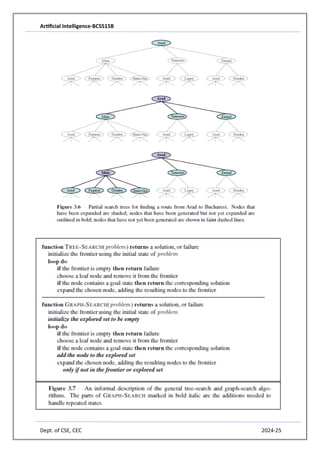
  • 9. Artificial Intelligence-BCS515B Dept. of CSE, CEC 2024-25 • Initial state: This is specified by the user’s query. • Actions: Take any flight from the current location, in any seat class, leaving after the current time, leaving enough time for within-airport transfer if needed. • Transition model: The state resulting from taking a flight will have the flight’s destination as the current location and the flight’s arrival time as the current time. • Goal test: Are we at the final destination specified by the user? • Path cost: This depends on monetary cost, waiting time, flight time, customs and immigration procedures, seat quality, time of day, type of airplane, frequent-flyer mileage awards, and so on. 2) Route-finding problems 3) GPS-based navigation systems, Google maps 4) Touring problems 5) Real-World Search Problems 6) TSP (traveling salesperson problem) 7) VLSI layout problems 8) Robot navigation problems 9) Automatic assembly sequencing 10) Internet searching 11) Searching paths in metabolic networks in 12) Bioinformatics 13) protein design 3.3 SEARCHING FOR SOLUTIONS: Asolution is an action sequence, so search algorithms work by considering various possible action sequences. The possible action sequences starting at the initial state form a search tree with the initial state at the root; the branches are actions and the nodes correspond to states in the state space of the problem. Figure 3.6 shows the first few steps in growing the search tree for finding a route from Arad to Bucharest. The root node of the tree corresponds to the initial state, In(Arad).The first step is to test whether this is a goal state. (Clearly it is not, but it is important to check so that we can solve trick problems like “starting in Arad, get to Arad.”) Then we need to consider taking various actions. We do this by expanding the current state; that is, applying each legal action to the current state, thereby generating a new set of states. In this case, we add three branches from the parent node In(Arad) leading to three new child nodes: In(Sibiu), In(Timisoara), and In(Zerind). We check to see whether it is a goal state (it is not) and then expand it to get In(Arad), In(Fagaras), In(Oradea), and In(RimnicuVilcea). We can then choose any of these four or go back and choose Timisoara or Zerind. Each of these six nodes is a leaf node, that is, a node with no children in the tree. The set of all leaf nodes available for expansion at any given point is called the frontier. (Many authors call it the open list, which is both geographically less evocative and less accurate, because other data structures are better suited than a list.)
  • 11. Artificial Intelligence-BCS515B Dept. of CSE, CEC 2024-25 As the saying goes, algorithms that forget their history are doomed to repeat it. The way to avoid exploring redundant paths is to remember where one has been .To do this, we augment the algorithm with a data structure called the explored set (also known as the closed list), which remembers every expanded node. Newly generated nodes that match previously generated nodes—ones in the explored set or the frontier—can be discarded instead of being added to the frontier. The new algorithm, called GRAPH-SEARCH, is shown informally in Figure 3.7. The specific algorithms in this chapter draw on this general design. 3.3.1 Infrastructure for search algorithms Search algorithms require a data structure to keep track of the search tree that is being constructed. For each node n of the tree, we have a structure that contains four components: • n.STATE: the state in the state space to which the node corresponds; • n.PARENT: the node in the search tree that generated this node; • n.ACTION: the action that was applied to the parent to generate the node;
  • 12. Artificial Intelligence-BCS515B Dept. of CSE, CEC 2024-25 • n.PATH-COST: the cost, traditionally denoted by g(n), of the path from the initial state to the node, as indicated by the parent pointers. The node data structure is depicted in Figure 3.10. Notice how the PARENT pointer string the nodes together into a tree structure. These pointers also allow the solution path to be extracted when a goal node is found; we use the SOLUTION function to return the sequence of actions obtained by following parent pointers back to the root. The appropriate data structure for this is a queue. The operations on a queue are as follows: • EMPTY?(queue) returns true only if there are no more elements in the queue. • POP(queue) removes the first element of the queue and returns it. • INSERT(element, queue) inserts an element and returns the resulting queue. Queues are characterized by the order in which they store the inserted nodes. Three common variants are the first-in, first-out or FIFO queue, which pops the oldest element of the queue;the last-in, first-out or LIFO queue (also known as a stack), which pops the newest element of the queue; and the priority queue, which pops the element of the queue with the highest priority according to some ordering function. 3.3.2 Measuring problem-solving performance We can evaluate an algorithm’s performance in four ways: • Completeness: Is the algorithm guaranteed to find a solution when there is one? • Optimality: Does the strategy find the optimal solution, as defined on page 68? • Time complexity: How long does it take to find a solution? • Space complexity: How much memory is needed to perform the search?
  • 13. Artificial Intelligence-BCS515B Dept. of CSE, CEC 2024-25 Complexity is expressed in terms of three quantities: b, the branching factor or maximum number of successors of any node; d, the depth of the shallowest goal node (i.e., the number of steps along the path from the root); and m, the maximum length of any path in the state space. m: maximum depth of the state space (may be ∞). To assess the effectiveness of a search algorithm, we can consider just the search cost—which typically depends on the time complexity but can also include a term for memory usage—or we can use the total cost, which combines the search cost and the path cost of the solution found. 3.4 UNINFORMED SEARCH STRATEGIES The Uninformed Search term means that the strategies have no additional information about states beyond that provided in the problem definition. All they can do is generate successors and distinguish a goal state from a non-goal state. All search strategies are distinguished by the order in which nodes are expanded. Strategies that know whether one non-goal state is “more promising” than another are called informed search or heuristic search strategies. • Breadth-first search (BFS) • Uniform-cost search • Depth-first search (DFS) • Depth-limited search • Iterative deepening search • Bidirectional Search 3.4.1 Breadth-first search • The root node is expanded first • Then all successors of the root node are expanded • Then all their successors and so on • In general, all the nodes of a given depth are expanded • before any node of the next depth is expanded. • Uses a standard queue as data structure. Pseudocode is given in Figure 3.11. Figure 3.12 shows the progress of the search on a simple binary tree. Imagine searching a uniform tree where every state has b successors. The root of the search tree generates b nodes at the first level, each of which generates b more nodes, for a total of b2 at the second level. Each of these generates b more nodes, yielding b3 nodes at the third level, and so on. Now suppose that the solution is at depth d. In the worst case, it is the last node generated at that level. Then the total number of nodes generated is
  • 14. Artificial Intelligence-BCS515B Dept. of CSE, CEC 2024-25 Two lessons can be learned from Figure 3.13. First, the memory requirements are a bigger problem for breadth-first search than is the execution time. One might wait 13 days for the solution to an important problem with search depth 12, but no personal computer has the petabyte of memory it would take. Fortunately, other strategies require less memory. The second lesson is that time is still a major factor. If your problem has a solution at depth 16, then (given our assumptions) it will take about 350 years for breadth-first search (or indeed any uninformed search) to find it. In general, exponential-complexity search problems cannot be solved by uninformed methods for any but the smallest instances.
  • 15. Artificial Intelligence-BCS515B Dept. of CSE, CEC 2024-25 3.4.2 Uniform-cost search • Modification to BFS generates Uniform-cost search, which works with any step-cost function ( edge weights/costs): • UCS expands the node n with lowest summed path cost g(n). • To do this, the frontier is stored as a priority queue. (Sorted list data structure, better heap data structure). • The goal test is applied to a node when selected for expansion (not when it is generated). • Also a test is added if a better node is found to a node on the frontier. The algorithm is shown in Figure 3.14.
  • 16. Artificial Intelligence-BCS515B Dept. of CSE, CEC 2024-25 The Modifications come into play in the example shown in Figure 3.15, where the problem is to get from Sibiu to Bucharest. The Uniform Search is similar to Dijkstra’s algorithm. It requires that all step costs are non-negative. It may get stuck if there is a path with an infinite sequence of zero cost steps. Otherwise it is complete. 3.4.3 Depth-first search • DFS alwas expands the deepest node in the current frontier of the search tree. • It uses a stack (LIFO queue last in first out) • DFS is frequently programmed recursively, then the program call stack is the LIFO queue. • DFS is complete, if the graph is finite. • The tree search version of DFS is complete on a finite tree, if a test is included whether the node has already been visited • DFS is incomplete on infinite trees or graphs. • DFS has time complexity O(bm ), if m is the maximum depth of any node (may be infinite). • DFS has space complexity of O(b m) • As an alternative to the GRAPH-SEARCH-style implementation, it is common to implement depth-first search with a recursive function that calls itself on each of its children in turn. In Figure 3.16, depth first search will explore the entire left subtree even if node C is a goal node. If node J were also a goal node, then depth-first search would return it as a solution instead of C, which would be a better solution; hence, depth-first search is not optimal. The time complexity of depth-first graph search is bounded by the size of the state space (which may be infinite, of course). A depth-first tree search, on the other hand, may generate all of the O(bm) nodes in the search tree, where m is the maximum depth of any node; this can be much greater than the size of the state space. Note that m itself can be much larger than d (the depth of the shallowest solution) and is infinite if the tree is unbounded. A variant of depth-first search called backtracking search uses still less memory. In backtracking, only one successor is generated at a time rather than all successors; each partially expanded node remembers which successor to generate next. In this way, only O(m) memory is needed rather than O(bm). Backtracking search facilitates yet another memory-saving (and time-saving) trick: the idea of generating a successor by modifying the current state description directly rather than copying it first. This reduces the memory requirements to just one state description and O(m) actions.
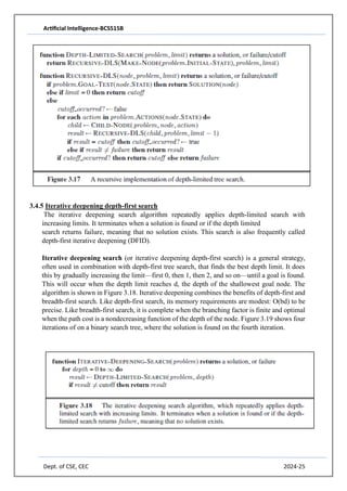
  • 17. Artificial Intelligence-BCS515B Dept. of CSE, CEC 2024-25 3.4.4 Depth-limited search • The failure of DFS in infinite search spaces can be prevented by giving it a search limit l .This approach is called depth limited search • Unfortunately, it is not complete if we choose l < d, where d is the depth of the goal node. • This happens easily, because d is unknown. • Depth-limited search has time complexity O(b l). • It has space complexity of O(b l). • However, in some applications we know a depth limit (# nodes in a graph, maximum diameter, …) • Depth-first search can be viewed as a special case of depth-limited search with l =∞.
  • 18. Artificial Intelligence-BCS515B Dept. of CSE, CEC 2024-25 3.4.5 Iterative deepening depth-first search The iterative deepening search algorithm repeatedly applies depth-limited search with increasing limits. It terminates when a solution is found or if the depth limited search returns failure, meaning that no solution exists. This search is also frequently called depth-first iterative deepening (DFID). Iterative deepening search (or iterative deepening depth-first search) is a general strategy, often used in combination with depth-first tree search, that finds the best depth limit. It does this by gradually increasing the limit—first 0, then 1, then 2, and so on—until a goal is found. This will occur when the depth limit reaches d, the depth of the shallowest goal node. The algorithm is shown in Figure 3.18. Iterative deepening combines the benefits of depth-first and breadth-first search. Like depth-first search, its memory requirements are modest: O(bd) to be precise. Like breadth-first search, it is complete when the branching factor is finite and optimal when the path cost is a nondecreasing function of the depth of the node. Figure 3.19 shows four iterations of on a binary search tree, where the solution is found on the fourth iteration.
  • 19. Artificial Intelligence-BCS515B Dept. of CSE, CEC 2024-25 The total number of nodes generated in the worst case is 3.4.6 Bidirectional search The idea behind bidirectional search is to run two simultaneous searches—one forward from the initial state and the other backward from the goal—hoping that the two searches meet in the middle (Figure 3.20). The motivation is that bd/2 + bd/2 is much less than bd , or in the figure, the area of the two small circles is less than the area of one big circle centered on the start and reaching to the goal. The time complexity of bidirectional search using breadth-first searches in both directions is O(bd/2 ). The space complexity is also O(bd/2 ). We can reduce this by roughly half if one of the two searches is done by iterative deepening, but at least one
  • 20. Artificial Intelligence-BCS515B Dept. of CSE, CEC 2024-25 of the frontiers must be kept in memory so that the intersection check can be done. This space requirement is the most significant weakness of bidirectional search. Advantage: delays exponential growth by reducing the exponent for time and space complexity in half. Disadvantage: At every time point the two fringes must be compared. This requires an efficient hashing data structure Bidirectional search also requires to search backward (predecessors of a state). This is not always possible. 3.4.7 Comparing uninformed search strategies Figure 3.21 compares search strategies in terms of the four evaluation criteria set forth in Section 3.3.2. This comparison is for tree-search versions. For graph searches, the main differences are that depth-first search is complete for finite state spaces and that the space and time complexities are bounded by the size of the state space.