SlideShare a Scribd company logo
Big Data Analytics Tools./.DS_Store
__MACOSX/Big Data Analytics Tools./._.DS_Store
Big Data Analytics Tools./ Final Exam/PROJECT - BETTER
UNDERSTAND ATTRITION.docx
FINAL EXAM – EXERCISE – To Better Understand Attrition.
This is a final project – you are going to exam the HR-
BalanceSheet dataset and write a short report on what you
found. I will guide you through the analysis, but as we go
through the analysis you are going to need to capture data for
the final report.
1. Load the dataset into Statistica
2. Generate Histograms for all of the data
a. Make notes on what you observe from the histograms. Can
you learn anything about the business from these histograms?
b. Capture all of the histograms.
3. Now generate a correlation matrix to see if any variables are
highly correlated. If variables are highly correlated and you
are doing a supervised method (e.g., decision tree), then one of
them must be omitted from the analysis. Do you know why?
Statistics->Nonparametrics->Correlations Okay.
Now select ALL of the variables and select “Spearman rank R”.
4. Let’s copy this out to Excel.
a. Open a blank Excel file
b. Go to Statistica – the output correlation matrix –
i. Hit Ctrl – A - this will select everything.
ii. Right Click - select “Copy with Headers”
iii. Go To Excel – select Paste
5. Select all of the numbers in Excel
a. Go To Conditional Formatting
i. Highlight all values greater than 0.70
6. This tells you the values that are highly correlated. Record
what they are – these cannot be used in a supervised modeling
exercise together. For example, JobLevel and
TotalWorkingYears are highly correlated.
a. Make a list of all of the variables that are highly correlated
(>0.7).
BUSINESS PROBLEM: The company has employee data for
the last several years. In this data set we have a wide range of
data, including whether or not they left the company (i.e.,
Attrition). If Attrition is set to “Yes”, they left the company.
If Attrition is set to “No”, they did not leave the company.
The first thing we want to do is take a “high” level look at those
people who left the company.
Go to Selection Criteria – that is accessible through the Sel:Off
setting at the bottom of the Statistica window. Click on
“Sel:Off”
Set the selection criteria to Attribute = “Yes”.
7. Generate Histograms for all of the data
a. Make notes on what you observe from the histograms. Can
you learn anything about the business from these histograms?
b. Capture the histograms that tell you something about the
business.
Go back to the selection criteria and turn the Sel: back to “Off”.
8. Now build a decision tree (C&RT) to see if we can find out
what influences where or not individuals decide to leave the
company.
If you exclude the variables that are highly correlated, you can
generate a tree.
Generate a C&RT tree
Pick your variables (Quick)
· Attrition is your dependent variable
· Select the categorical and continuous variables that you
reasonably think could be an issue with respect to attrition.
· Select your response codes
· ALL
Don’t do anything on Classification (YET) – you may want to
go back and play with the classification weights – but, don’t do
that yet.
On the “Stopping” tab, change the minimum n to 20. This will
allow it to build a deeper tree.
Select V-fold cross validation on the Validation tab
Set Surrogate to 2 on the Advanced tab and hit OK.
Look at your tree –
Look at the Predicted Versus Observed – under classification.
Look at “Importance” on the Summary tab – this tells you which
variables have the greatest impact.
This is your initial tree ---
Now – the best you’re going to be able to do is get about 80%
accuracy on both Predicting yes and no.
So – play with it and see how good you can get it.
· Play with the classification costs
· You may try to create a stratified subsample using Attrition as
the strata variable
1
__MACOSX/Big Data Analytics Tools./ Final
Exam/._PROJECT - BETTER UNDERSTAND
ATTRITION.docx
Big Data Analytics Tools./ Final Exam/.DS_Store
__MACOSX/Big Data Analytics Tools./ Final
Exam/._.DS_Store
Big Data Analytics Tools./ Final Exam/FINAL EXAM -
2018.docx
FINAL EXAM NAME: _________________________
1. When we evaluate models we often discuss things like
predictive accuracy, speed, robustness, scalability, and
interpretability. Briefly discuss what is meant by
“interpretability” and why it is important.
2. You have been hired by the county government to help
automate a system to detect fraudulent spending by government
employees.
You have been given a database of transactions for the past 10
years to work with. Each record in the database contains all of
the details of each transaction as well as information related to
the particular employee. In this database accountants have
manually gone through the data and marked each transaction as
either “Good” or “Fraudulent”.
The goal – build a model based on the historical data that will
flag future transactions as either “Good” or “Fraudulent”. This
will eliminate the need for the accountants to have to go
through each transaction manually in the future. What type of
modeling technique (e.g., decision tree, association analysis,
clustering, etc.) would you use and why?
3. AT&T has been losing customers to Verizon. They want to
try to understand why this is the case. They have customer
records for the past 5 years that contain demographic
information (age, gender, etc.) for the customers, the type of
plan that they have, the number of interactions they have had
with customer support and whether or not those customers left
AT&T.
AT&T wants you to build a model that can be used to predict
whether or not a customer is going to leave and switch to
another provider. What type of technique (e.g., decision tree,
association analysis, clustering, etc.) would you use and why??
4. Kroger is trying to find ways to improve sales. They have
all of their receipts for the past 5 years. The receipts contain
information about what was purchased, who purchased, and the
date and time of the transaction.
You task is to analyze sales patterns and make recommendations
with respect to store layouts that, you hope, will increase sales.
What type of modeling technique (e.g., decision trees,
association analysis, clustering, etc.) would you use and why?
5. You work for a cable service provider. You provide a
variety of services for your customers. Your company provides
cable TV, home phone, security systems, and internet services.
Your customer base is very diverse. Your customers could be
male/female, young/old, single/married/married with children,
etc. You have a wide range of ethnic backgrounds and income
levels.
You want to make your marketing campaigns more effective.
This means targeting the right groups with the right messages
using the right media. (For example, marketing via social
media may be more or less effective for 18 year olds as
compared to 80 year olds).
You been tasked to use the customer database and determine
what the different customer segments are and what they look
like. Then, once you figure out what the unique groups are
you can go through and develop a targeted campaign for each
group. What type of modeling technique (e.g., decision trees,
association analysis, clustering, etc.) would you use to
determine the different market sectors and why?
Text and Web Analytics
6. When we do text analytics, we read in the data, we transform
the data into documents, and then we must generate a
term/document matrix. This term/document matrix is what we
use to perform analysis.
Generation of the term/document matrix involves some
processing of the document (see figure on the right).
Briefly describe each step and what it does.
a. Tokenize:
b. Transform Cases:
c. Filter Stopwords (English):
d. Filter Tokens by Length:
e. Stem (Porter):
7. Briefly describe what “Sentiment Analysis” is and how it
might be used by a company.
8. What is the difference between text mining and data mining?
9. FINAL EXAM – 2018 – BETTER UNDERSTAND
ATTRITION “projects”
Write me a short report that tells me the following (I’d like for
this report to be uploaded in a separate standalone word file and
look like something you would give an employer):
Business Scenario – write this like you worked for the company.
Tell me what the issue is you are exploring and why.
What you did and why you did it – just discuss the technique
you used, why it was appropriate and what you did. If you did
several iterations, let me know what the final configuration was.
I don’t need to know everything that went on – just what you
did to get the final results.
What you found – tell me everything you found/learned.
Include screen shots, graphs, etc. Anything appropriate to
communicate what you found. Do NOT show me everything
that was generated – just those things that support your
“findings”.
Recommendations - What impact this would have to the
business AND what your recommendations are for the business.
1
__MACOSX/Big Data Analytics Tools./ Final Exam/._FINAL
EXAM - 2018.docx
Big Data Analytics Tools./ Final Exam/HR-BalancedSheet.sta
__MACOSX/Big Data Analytics Tools./ Final Exam/._HR-
BalancedSheet.sta
Big Data Analytics Tools./Final Exam materials/1 BINS 4352 -
Association Analysis.pptx
Association Analysis
BINS 4352
Learning Objectives
Gain an understanding of how Association Analysis is used
Understand how Associations are created and how to
interpret/evaluate those Associations
Discuss and understand Association metrics – Lift, Support, and
Confidence
Gain familiarity with RapidMiner
Association Analysis
(Market Basket Analysis)
This is a widely used and, in many ways, one of the most
successful data mining algorithm.
It can be used to determines what products people purchase
together.
Uses
Stores can use this information to determine store layout and
product placement
Direct marketers can use this information to determine which
new products to offer to their current customers.
Inventory policies can be improved if reorder points reflect the
demand for the complementary products.
Any application where you are looking to see if there is a
pattern where strong associations are present
Parable Of “Beer And Diapers”
Customers who bought diapers at a grocery store between 5-
7pm also tend to by beer.
This is a good example of the business value present in big data
analytics.
More than a parable – it was the result of a study commissioned
by Osco in the 1990’s and represented a starting point in big
data analytics
The finding led to the notion that there is value in discovering
uncommon relationships in data can be used to drive business
value.
Association Rules for
Market Basket Analysis
Rules are written in the form “left-hand side implies right-hand
side” and an example is:
Yellow Peppers IMPLIES Red Peppers, Bananas
To make effective use of a rule, three numeric measures about
that rule must be considered:
(1) support
(2) confidence
(3) lift
Measures of Predictive Ability
Support and Confidence: An Illustration
A
B
C
A
C
D
B
C
D
A
D
E
B
C
ERULESUPPORTCONFIDENCELIFTA => D2/52/3(2/3)/(2/5) =
1.67C => A2/52/4(2/4)/(2/5) = 1.25A => C2/52/3(2/3)/(2/5) =
1.67B & C => D1/51/3(1/3)/(1/5) = 1.67
A Note On Lift
Lift is an interesting measurement and one that has undergone a
great deal of scrutiny
For our purposes we defined Lift as Confidence/Support
However, there are other ways to calculate this measure
Some have argued that one must take into account the frequency
of the observation
You don’t necessarily want a product that is in 100,000
transactions to be penalized over a product that is involved in
10 transactions simply due to the number of occurrences (or
visa versa)
As such – when looking at this value in a tool keep in mind that
it is the “relative” value that is important and not the “absolute”
value.
Market Basket Analysis Methodology
We first need a list of transactions and what was purchased.
Receipts from stores
This may have to be “reformatted” depending on the tool that
you’re using
Next, we choose a list of products to analyze, and tabulate how
many times each was purchased with the others.
The diagonals of the table shows how often a product is
purchased in any combination, and the off-diagonals show
which combinations were bought.
A Convenience Store Example
Consider the following simple example about five transactions
at a convenience store:
Transaction 1: Frozen pizza, cola, milk
Transaction 2: Milk, potato chips
Transaction 3: Cola, frozen pizza
Transaction 4: Milk, pretzels
Transaction 5: Cola, pretzels
These need to be cross tabulated and displayed in a table.
A Convenience Store Example (cont)
The diagonal shows how many times a product was purchased
(in any combination)
Pizza and Cola sell together more often than any other combo; a
cross-marketing opportunity?
Milk sells well with everything – people probably come here
specifically to buy it.Product BoughtPizza alsoMilk
alsoCola
alsoChips alsoPretzels
alsoPizza21200Milk13111Cola21301Chips01010Pretzels01102
Using The Results
The tabulations can immediately be translated into association
rules and the numerical measures computed.
Comparing this week’s table to last week’s table can
immediately show the effect of this week’s promotional
activities.
But, you need to be careful that the results were not impact by
some external event (e.g., bad weather)
Some rules are going to be trivial (hot dogs and buns sell
together) or inexplicable (toilet rings sell only when a new
hardware store is opened).
Using The Results
Barbie® => Candy
Forbes (Palmeri 1997) reported that a major retailer has
determined that customers who buy Barbie dolls have a 60%
likelihood of buying one of three types of candy bars. The
retailer was unsure what to do with this nugget. The online
newsletter Knowledge Discovery Nuggets invited suggestions
(Piatesky-Shapiro 1998)
Put them closer together in the store.
Put them far apart in the store.
Package candy bars with the dolls.
Package Barbie + candy + poorly selling item.
Raise the price on one, lower it on the other.
Barbie accessories for proofs of purchase.
Do not advertise candy and Barbie together.
Offer candies in the shape of a Barbie Doll.
Augmenting Data to Yield More Insights
The sales data can be augmented with the addition of virtual
items.
For example, we could record that the customer was new to us
or had children.
The transaction record might look like:
Item 1: Sweater Item 2: Jacket Item 3: New
This might allow us to see what patterns new customers have
versus existing customers.
Limitations to Market Basket Analysis
A large number of real transactions are needed to do an
effective basket analysis, but the data’s accuracy is
compromised if all the products do not occur with similar
frequency.
The analysis can sometimes capture results that were due to
some external event
For example:
The success of previous marketing campaigns (and not natural
tendencies of customers).
Weather or natural disaster.
Association Analysis in Rapidminer
The Dataset
The data is organized into “Transactions”
Each transaction represents a grocery store receipt
The items we are interested in
includeHerringBaguetteAvocadoHeinekenOlivesSardinesCorned
BeefPeppersSodaCrackerBourbonArtichokeCokeApplesChicken
HamTurkeyIce CreamSteakBordeaux
Data is coded where “YES” indicates that it was purchased and
“NO” indicates that it was not purchased
Running Assoication Analysis in Rapid Miner
Select
New Process
RadipMiner Studio Professional Main Menu
RapidMiner Studio is very similar in layout to SAS Enterprise
Miner
Design Pane – where you layout the analysis you want to run
Drag/Drop Objects from the Operator list into the Design Space
Importing Dataset
There are several ways to import data
I am going to read the Excel file that has pre-processed grocery
store receipt data
I drag the “Read Excel” operator into the design space.
Connect the inp port on the side of the design space to the fil
port on the operator
Many operators have 2 output ports – one for processed data
and the other for an original data “pass through”
Configuring The Read Excel Operator
Parameters associated with the Read Excel Operator appear on
the right side of the screen when the operator is selected.
Go to “Import Configuration”
Select The Excel File
Select the data file that you want to import
Select “Next”
Preview The Data
The file that you import can contain multiple sheets
At this point you can select the sheet and the range of cells that
you wish to import
The data file we are working with has 1 sheet and by default all
of the entries are selected
Select “Next”
Annotating Data
Now you have the opportunity to add annotations to the data
We don’t need to set an attribute name for this data set
Select “Next”
Selecting attribute types
RapidMiner tries to determine the types of the attributes from
the data.
For Association Analysis we need to set the types to either
“Binomial” or “Nominal”
I am going to select “Binomial”
Select “Next”
Finished !
Once all of the data types are changed to Binomial – Select
“Finish”
Attribute Selection
Next we need to select the attributes that will be used in the
analysis.
This can be found on the Operator Pane under Blending ->
Attributes -> Selection
Drag/Drop Select Attributes into the Design
Select Attributes
Connect the “out” port of Read Excel to the “exa” port on the
Select Attributes.
Select the Select Attributes Operator – the parameters for the
operator will appear on the right side of the screen.
Selecting Attributes
On the Parameters Pane
Select the “subset” Attribute filter type
Select “Select Attributes”
The Select Attributes dialog box appears
Select all of the attributes except for “Transaction”
This is an ID for the transaction and is not needed for the
analysis
FP-Growth (Frequency Calculations)
Next we drag/drop and FP-Growth operator into the design
Connect the “exa” port of Select Attributes to “exa” of FP-
Growth
The FP Growth operator determines the “frequent item sets”
A frequent item set denotes the items (products) in the set that
have been purchased together frequently (in a certain ratio of
transactions)
We also need to define the positive value (open advanced
parameters)
Create Association Rules
Drag/drop “Create Association Rules” from the Operator Pane
into the Design space.
Connect the “fre” (frequencies) of FP-Growth to “ite” of Create
Association Rules
Parameters driving the rule creation can be set (Confidence, lift,
… and Thresholds)
Ready To Run !
Connect the “rul” and “ite” ports of the Create Association
Rules operator to the output (res) of the design space.
Select “Run” -
Output
We get 2 sets of output
One tab is for the FP-Growth operator and show the Frequent
Item Sets
The other contains the Association Rules
The Frequency data shows you the support for every
combination of products in the data set
Associations Rules (Sorted By Support)
Association Rules (Sorted By Confidence)
Association Rules (Sorted By Lift)
Interpreting The Rules
Rule: IF (turkey, baguette) THEN (ham, olives)
Support: The percentage of the time that the rule was true
26.7% of the time the basket contained both (turkey,baguette)
and (ham, olives)
Confident: The percentage of the time that the baskets that did
contain (turkey, baguette) also contained (ham, olives)
85% of the time when the basket contained (turkey, baguette) it
also contained (ham, olives)
Lift: is the relative measure that looks at how many times
Confidence is larger than the expected level (similar to what we
discussed earlier – better than a baseline model)
Greater than 1 is desired
The larger the value the better
Association Analysis in Statistica
Same Data File
Reformatted data just a little for Statistica (in Excel)
Each line contains what was sold for that transaction
Link Analysis
Go to Data Mining -> Link Analysis
Select Non-sequential association analysis
Select Variables as we have done in the past
Transaction – is the Transaction ID
Food items – are Multi-response variables
Database Selection
If you run the analysis multiple times, you may have to select a
database name.
This should only be the case if you exit the tool, reload data,
and try to run again.
Select “OK” and run the analysis
Results
Association Rules
Frequency Itemsets
Rule Graph
Web Graph
Questions?
__MACOSX/Big Data Analytics Tools./Final Exam
materials/._1 BINS 4352 - Association Analysis.pptx
Big Data Analytics Tools./Final Exam materials/2 BINS 4352-
Data Preparation.pptx
Data Preparation
Objectives
Provide a perspective on how data may have to be prepared for
a given Analytics task
Understand the relationship between the data mining technique
and the business problem being addressed
Gain an understanding of the types of data issues that might be
found
Understand options when it comes to “fixing” or “addressing”
data issues
Understand what impact “uncleaned” data may have on the
analysis
Provide a “practical” and “applied” understanding of statistical
concepts
Data in Data Mining
Data: a collection of facts usually obtained as the result of
experiences, observations, or experiments.
Data may consist of numbers, words, images, …
Data: lowest level of abstraction (from which information and
knowledge are derived).
Nominal – mutually exclusive, but not order categories (e.g.,
male, female)
Ordinal – order matters (e.g., Freshman, Sophomore, Junior,
Senior).
Interval – measure where difference between two variables is
meaningful.
Ratio – all the properties of Interval, but with an absolute 0
which means complete lack of that variable.
3
Inspecting Data and Preparation in Excel
Preparing Data In Excel
We are looking for anomalies in the data
Missing values
Values out of a defined range
Etc.
Once we find these values – we can
Repair the data
Impute missing values
Delete the response
5
DATA Dictionary
6
The data dictionary tab describes everything that is in the data
set
If you download a data set from the Internet, it will often
include a data dictionary in a separate file.
Raw data
7
The raw data is the data as it was collected.
There have been no changes/modifications to the data at this
point.
Highlight
Blanks
8
All of the data was selected in the spreadsheet
Go to FIND & SELECT in Excel (on the HOME Tab)
Select “GO TO SPECIAL”
Select “Blanks”
Then set the fill color to RED
Analyze Row / Columns
9
The raw data is the data as it was collected.
There have
been no changes/modifications to the
data at this point.
Count non-blank responses
Calculate the frequency of the “expected values”
Calculate difference from the means
Calculate single answer bias
How To Handle Anomalies In The Data
Decide what your going to do about the anomalies you found in
the data.
Filter values
Repair the file (impute values)
Leave them alone
Delete responses
Etc.
If you are going to “change” data or “delete” data, move the
original values to a separate sheet.
You are documenting what you did
This makes it easier to “undo” your change if you need to.
11
Statistica
Data
This sheet contains the “cleaned” data that you’re going to load
into Statistica for further analysis.
The excel manipulation was intended to address the “obvious”
problems
Graphical Inspection Credit Scoring Data
in Statistica
Application
As we have discussed practically all data will need some
preparation
More over – that preparation may be slightly different based on
the application and the type of analysis that you are doing
It is important to have a good understanding of both the data
and what you’re trying to accomplish through the data mining
process
Data preparation
Handling missing data and outliers
Selecting important variables
Sampling
Data preparation is specific to BOTH the data set and the task.
The preparation method and decisions made during data
preparation may change if either change
Application For Credit Scoring Data
Business Need
A financial institution has data about their past customers.
These customers are classified as either good or bad credit risks
based on their history with the institution.
The classification (good/bad) is based on whether or not the
loan payment was delinquent and the magnitude of the loss
A financial institution needs a way to decide if and how much
credit to extend to customers who apply for loans.
Business goal: reduce the losses due to bad loans
Goals of the data mining process
Determine the variables that are best predictors of credit risk
Find a high performance predictive model that classifies
customers
Deploy that model to make decisions on future credit
applications
Update the model as more data is collected
Credit Scoring Data Set
We are going to explore the credit scoring data set
This data will be used to explore
Data preparation
Classification
Try to keep in mind – this will be a “classification exercise”.
It can be applied to different data sets and domains where
classification is appropriate
Examine the dataDataTypeCredit ratingCategoricalBalance of
current accountCategoricalDuration of
creditContinuousPayment of previous creditCategoricalPurpose
of creditCategoricalAmount of creditContinuousValue of
savings CategoricalEmployed by current
employerCategoricalInstallment in % of available
incomeCategoricalMarital
statusCategoricalGenderCategoricalLiving in current household
forCategoricalMost valuable
assetCategoricalAgeContinuousFurther running
creditsCategoricalType of apartmentCategoricalNumber of
previous credits at this
bankCategoricalOccupationCategoricalTrainTestcategorical
Credit Scoring
Start by looking at the credit scoring application and the
business need
Review the variables in the credit risk data set
Discuss the next steps for the data mining process
Classification
Classification can be used to classify a variable with 2 or more
groups
Find the probability of a particular predicted classification.
For example:
Loan denied
Loan approved
Examine The Data
Below is the data in Statistica
It was opened by FILE-> OPEN
Look At Some Histograms Of The Data
Histograms
Credit rating is the dependent variable – it is the one we want to
make predictions for
Notice that there have been more than twice as many customers
with good credit as compared to bad
This may mean that we need to adjust our sample to keep the
analysis from being “good” credit biased
Histograms
Here we have the number of previous credits at the bank
5-6 and 7 or more are relatively small compared to the other
categories
Hence, we may want to recode the data to have a 5 or more
category
This is a good general rule of thumb
Remaining Variables
Remaining Variables
Note the majority of customers either have no previous credit or
have paid back their previous loans
Remaining Variables
Remaining Variables
Remaining Variables
Note: that there have been more than twice as many male
customers as female customers
Remaining Variables
Remaining Variables
Age is interesting in that you would expect that customers need
to be at least 18 years old to apply for credit, so we need to
make sure that is the case in the 15-20 year old group
Remaining Variables
Remaining Variables
Next Steps
We have stated the business goals and have data available to do
the analysis
We have visually inspected the data in order to gain a high-level
understanding of the data
We still need to do more work here
But, we have identified our dependent variable (Credit Risk)
and the potential predictor variables
We need to continue exploring the data and look at things that
we can do to prepare the data for analysis
Further Analysis
Go to the interactive drill down tool
Select the “Drill Variables”
Select “Payment of Previous Credits”
Drill Down
Select “No Previous Credits”
Go back to the “Drill down variables” and select “Number of
Previous Payments”
Select “Brush”
Previous payment
So here we have an apparent contradiction.
We have drilled down to look at customers where the Payment
of Previous Credits = no previous credits
But, yet the number of previous credits at this bank has values
for 2-4, 5-6, and 7 or more?
Scatter Plot Matrix
A scatter plot matrix can help us look for potential outliers
Scatter Plot Matrix
We can combine this with the Drill Down and look at scatter
plots of all of the continuous variables with respect to those
where the Payment of Previous Credits = no previous credits
Scatter Plot – Duration Of Credit Vs Amount Of Credit
Scatter Plot
We can look for outliers here
If we know that there is a maximum loan amount, then we can
remove those that are greater than that value
If we know that there is a maximum duration, we can remove all
of those that are greater than that
Other Graphical Techniques
Box Plots
A box plot or boxplot is a convenient way of graphically
depicting groups of numerical data through their quartiles.
Box plots may also have lines extending vertically from the
boxes (whiskers) indicating variability outside the upper and
lower quartiles, hence the terms box-and-whisker plot and box-
and-whisker diagram.
Outliers may be plotted as individual points.
Box plots are non-parametric: they display variation in samples
of a statistical population without making any assumptions of
the underlying statistical distribution.
The spacing between the different parts of the box indicate the
degree of dispersion (spread) and skewness in the data, and
show outliers.
There Are Several Variations of Box Plots
The “box” :
The band inside the box is the second quartile (the median).
Statistica gives you the option to make this the “mean”
The ends of the “whiskers” can represent several possible
alternative values:
Min and Max of all of the data
Lowest datum still within 1.5 interquartile range (IQR) of the
lower quartile, and the highest datum still within 1.5 IQR of the
upper quartile (often called the Tukey boxplot)
one standard deviation above and below the mean of the data
Etc.
Box Plot
These may seem more “primitive” than a histogram, but they do
have some advantages
They take up less space – so they are particularly useful in
comparing distributions among several groups
The number and width of bins can greatly impact the appearance
of a histogram
Box plots are particularly good at identifying outliers in
continuous data
Box Plots in Statistica
Go to “GRAPHS” and select “Box Plots”
Graph Type
Box Whiskers
Regular (will give you 1 variable per graph)
Multiple (will give you 1 graph with all on it”
Variables – where you select the variables for analysis
Box Plots
Leave the defaults for Grouping Intervals
Middle point
Value – median
Style – determines the graphics that show the median in the box
Box Plots
I have re-selected “Multiple” Graph type
I prefer the median be marked with a “Line”
Box Plots
The graph is fairly crowded – but, I can see outliers that are
identified by the small circles.
I will re-run this with fewer variables to see if we can see it
better
Box Plots
Now we can more clearly see where the outliers are in the data
set.
These need to be examined for deletion
Next we will look at this in SPSS
Marking The Outliers
Right clicking on the outliers will pull up a menu where you can
tell Statistica to “Mark the Outliers”
SPSS – Box Plots
The data is loaded into
SPSS
This can be done by loading the same file we used for Statistica
Go to “Graphs” and then to “Legacy Dialogs” and Select “Box
Plots”
Select “Simple” and “Summaries of separate variables”
SPSS – Box Plots
Next we select the variables and move them to the “Boxes
Represent” area
Select “OK”
SPSS – Box Plots
We see output very similar to Statistica.
The outliers are marked with “o” on the graph
In SPSS the default is to display the “number” of the response
with the outlier
Inspecting Outliers
In Box Plot
We want to be very conservative when identifying responses as
“outliers”
Count how many “outliers” each respondent has
For example, response 188 has 3 outliers, 187 has 4 outliers,
and so on.
I may delete 1 or 2 responses that have a “large” number of
outliers and then rerun the box plot.
This will cause things to shift a bit
I then iterate until I’m happy with the data.
Leaving outliers in the data is fine – this may be a “true”
response
QUESTIONS?
Data
CategoricalNumerical
NominalOrdinalIntervalRatio
Histogram of Credit Rating
CreditScoring 19v*1000c
Credit Rating = 1000*1*Normal(Location=0.7, Scale=0.4585)
bad good
Credit Rating
0
100
200
300
400
500
600
700
800
No of obs
Histogram of Number of previous credits at this bank
CreditScoring 19v*1000c
Number of previous credits at this bank =
1000*1*Normal(Location=1.407, Scale=0.5777)
one 2- 4 5- 6 7 or more
Number of previous credits at this bank
0
100
200
300
400
500
600
700
No of obs
Histogram of Balance of Current Account
CreditScoring 19v*1000c
Balance of Current Account = 1000*1*Normal(Location=2.577,
Scale=1.2576)
no running account
no balance
<= $300
>$300
Balance of Current Account
0
50
100
150
200
250
300
350
400
450
No of obs
Histogram of Duration of Credit
CreditScoring 19v*1000c
Duration of Credit = 1000*10*Normal(Location=20.903,
Scale=12.0588)
-1001020304050607080
Duration of Credit
0
50
100
150
200
250
300
350
400
No of obs
Histogram of Payment of Previous Credits
CreditScoring 19v*1000c
Payment of Previous Credits = 1000*1*Normal(Location=2.545,
Scale=1.0831)
hesistant
problematic running accounts
no previous credits
no problems with current credits
paid back
Payment of Previous Credits
0
100
200
300
400
500
600
No of obs
Histogram of Purpose of Credit
CreditScoring 19v*1000c
Purpose of Credit = 1000*1*Normal(Location=2.828,
Scale=2.7444)
other
new car
used car
furniture
television
household appliances
repair
education
vacation
retraining
business
Purpose of Credit
0
20
40
60
80
100
120
140
160
180
200
220
240
260
280
300
No of obs
Histogram of Amount of Credit
CreditScoring 19v*1000c
Amount of Credit = 1000*5000*Normal(Location=4579.7472,
Scale=3951.8525)
-$5,000.00
$0.00
$5,000.00
$10,000.00
$15,000.00
$20,000.00
$25,000.00
$30,000.00
Amount of Credit
0
100
200
300
400
500
600
700
800
No of obs
Histogram of Value of Savings
CreditScoring 19v*1000c
Value of Savings = 1000*1*Normal(Location=2.105,
Scale=1.58)
no savings
<140 140-700 700-1400 >1400
Value of Savings
0
100
200
300
400
500
600
700
No of obs
Histogram of Employed by Current Employer for
CreditScoring 19v*1000c
Employed by Current Employer for =
1000*1*Normal(Location=3.384, Scale=1.2083)
unemployed
<1 year 1-5 years 5-8 years > 8 years
Employed by Current Employer for
0
50
100
150
200
250
300
350
400
No of obs
Histogram of Installment in % of Available Income
CreditScoring 19v*1000c
Installment in % of Available Income =
1000*1*Normal(Location=2.973, Scale=1.1187)
> 35 25-35 15- 25 < 15
Installment in % of Available Income
0
100
200
300
400
500
No of obs
Histogram of Marital Status
CreditScoring 19v*1000c
Marital Status = 1000*1*Normal(Location=2.682,
Scale=0.7081)
divorced/living apart
divorced/living apart/married
single
married/widowed
Marital Status
0
100
200
300
400
500
600
No of obs
Histogram of Gender
CreditScoring 19v*1000c
Gender = 1000*1*Normal(Location=1.31, Scale=0.4627)
male female
Gender
0
100
200
300
400
500
600
700
800
No of obs
Histogram of Living in Current Household for
CreditScoring 19v*1000c
Living in Current Household for =
1000*1*Normal(Location=2.845, Scale=1.1037)
< 1 year 1-5 years 5-8 years >8 years
Living in Current Household for
0
50
100
150
200
250
300
350
400
450
No of obs
Histogram of Most Valuable Assets
CreditScoring 19v*1000c
Most Valuable Assets = 1000*1*Normal(Location=2.358,
Scale=1.0502)
no assets
car
life insurance
ownership of house or land
Most Valuable Assets
0
50
100
150
200
250
300
350
No of obs
Histogram of Age
CreditScoring 19v*1000c
Age = 1000*5*Normal(Location=33.544, Scale=11.3498)
1015
20
253035404550556065707580
Age
0
20
40
60
80
100
120
140
160
180
200
220
240
260
No of obs
Histogram of Further running credits
CreditScoring 19v*1000c
Further running credits = 1000*1*Normal(Location=2.675,
Scale=0.7056)
at other banks
at department store
no further running credits
Further running credits
0
100
200
300
400
500
600
700
800
900
No of obs
Histogram of Type of Apartment
CreditScoring 19v*1000c
Type of Apartment = 1000*1*Normal(Location=1.928,
Scale=0.5302)
free rented owned
Type of Apartment
0
100
200
300
400
500
600
700
800
No of obs
Histogram of Number of previous credits at this bank
CreditScoring 19v*1000c
Number of previous credits at this bank =
1000*1*Normal(Location=1.407, Scale=0.5777)
one 2- 4 5- 6 7 or more
Number of previous credits at this bank
0
100
200
300
400
500
600
700
No of obs
Histogram of Occupation
CreditScoring 19v*1000c
Occupation = 1000*1*Normal(Location=2.904, Scale=0.6536)
unskilled with no permanant residence
unskilled with permanant residence
skilled employee
executive/self-employed
Occupation
0
100
200
300
400
500
600
700
No of obs
Histogram for brushing: Number of previous credits at this bank
N Total: 1000, Selected: 530
Payment of Previous Credits = no previous credits
050100150200250300350400450500
Number of counts
one
2- 4
5- 6
7 or more
Number of previous credits at this bank
Correlations
N Total: 1000, Selected: 1000
Duration of Credit
Amount of Credit
Age
Correlations
N Total: 1000, Selected: 530
Payment of Previous Credits = no previous credits
Duration of Credit
Amount of Credit
Age
Scatterplot of Amount of Credit against Duration of Credit
CreditScoring 19v*1000c
Amount of Credit = 298.4367+204.818*x
01020304050607080
Duration of Credit
-$2,000.00
$0.00
$2,000.00
$4,000.00
$6,000.00
$8,000.00
$10,000.00
$12,000.00
$14,000.00
$16,000.00
$18,000.00
$20,000.00
$22,000.00
$24,000.00
$26,000.00
$28,000.00
Amount of Credit
Box Plot of multiple variables
1-ORIGINAL-FULL-DATASET-WALK-THROUGH 61v*261c
Median; Box: 25%-75%; Whisker: Non-Outlier Range
Median
25%-75%
Non-Outlier Range
Outliers
Extremes
CCSC_1
CCOC_1
CCAC_1
CCAC_6
HCA_5
UCA_4
PEOU_3
PU_4
PP_5
BI_5
PF_4
PIIT_1
0
1
2
3
4
5
6
7
8
Box Plot of multiple variables
1-ORIGINAL-FULL-DATASET-WALK-THROUGH 61v*261c
Median; Box: 25%-75%; Whisker: Non-Outlier Range
Median
25%-75%
Non-Outlier Range
Outliers
Extremes
UCA_1
UCA_3
UCA_5
PEOU_1
PEOU_3
PU_1
PU_3
PP_1
PP_3
PP_5
0
1
2
3
4
5
6
7
8
__MACOSX/Big Data Analytics Tools./Final Exam
materials/._2 BINS 4352- Data Preparation.pptx
Big Data Analytics Tools./Final Exam materials/2 BINS 4352 -
Cluster Analysis.pptx
Cluster Analysis
Cluster Analysis - Review
Outline
What is it? What is a cluster?
How is it different from a decision tree?
What is distance and linkage?
What is hierarchical clustering?
What is scree plot and denogram?
What is non-hierarchical clustering (k-means)?
How to learn it in detail?
3
Simple Case
StudyStudentPhysicsCalculusJoe1520Bill2015Paula2621Jane44
52Jack5045Carlos5738Carla8085Russell9088Eddie9898
4
If we look at the student data on the left, we can easily see a
pattern emerging
There are natural groupings of students that seem to be apparent
in the data.
Plotting these on a 2-dimensional scatter plot makes it more
visible
Similarities And Dissimilarities
If we look at the objects in any one of the groupings, they are
all very similar to the other objects in that grouping
Also, if we look at any one object in a grouping, it is very
dissimilar to any object in another grouping
This give rise to the notion of:
Homogeneous within and Heterogeneous across based on
characteristics
Clusters
These groupings are clusters
They represent a “natural grouping of similar objects” based on
a collection of input parameters
Now, if you add a third or forth dimension (e.g., English,
History), then the clusters may change
However, the way in which they are constructed is the same
Clusters
Clusters
There is no objective function (i.e., an equation to be optimized
given certain constraints with variables that need to be
minimized or maximized such as trying to express a business
goal in mathematical terms)
There is no dependent variable
This is sometimes called subjective segmentation
The segmentation is developed on its own based on the values
of the input variables
It is called a unsupervised learning technique.
Once the segments are developed
They need to be understood
You need to decide how you are going to deal with the segments
that have emerged
How Is This Different From A Decision Tree
Decision tree technique requires a clearly defined dependent
variable
For example, GOOD/BAD credit
The technique is based on identifying those variables
(characteristics) which are closely associated with the
dependent variable.
Distances
Distances (cont)
Paula
Bill
Joe
Jane
Jack
Carlos
Carla
Russell
Eddie
Distance Between 2 Clusters
Sometimes called the linkage function: intermediate cluster
distance
How do you calculate the distance between 2 clusters
Big Data Analytics Tools..DS_Store__MACOSXBig Data Analyti.docx
Single linkage
Calculate the distance between each point in one cluster to each
point in the neighboring cluster and then find the shortest
distance.
Complete linkage
Similar to single linkage – except we look for the furthest
distance
Centroid distance
Calculate the “center” of each cluster and then calculate the
distance between centroids
Hierarchical Clustering
Used when you have a small number of observations (usually
hundreds)
You can not use this method for a large dataset because it
becomes computationally impractical
The way this works is to join objects (cases) together into
successively larger clusters using some measure of similarity or
distance
During the clustering process it shows how the clusters are
formed
The result of the clustering is the hierarchical tree
In SAS this is done by using the “proc cluster” command
In Statistica this is called Joining or Tree Clustering
Hierarchical Clustering
We begin by each case in a cluster by itself
In each step we slowly “relax” the criterion which defines
“uniqueness”
In other words, we lower the threshold by what it means to
declare two or more objects within the same cluster
As a result we group more and more objects together and each
“layer” consists of increasingly dissimilar objects
In the last step – all objects are grouped together into a single
cluster
Scree Plot
When we look at a scree plot what we have is the “within
cluster variance”
Total variance = between variance + within variance
The “elbow” in the graph indicates the optimal number of
clusters
When the number of clusters = 1, the within group variance =
total variance
Dendogram
When the data contain a clear structure in terms of clusters,
then its structure is often reflected in the hierarchical tree
The result of a successful analysis is that you can detect and
interpret the structure by looking at the branches
Hierarchical Clustering - Students
Everything starts out in a cluster by itself
Find the closest objects.
Merge those into a cluster.
Recalcuate distances (from center of new cluster)
Find the closest objects.
Merge those into a cluster.
Recalcuate distances (from center of new cluster)
Joe Bill Paula
Jack
Jane
…
K-means Clustering
Non-hierarchical
Used when you have a large number of observations
You decide up front how many clusters you need (k)
K-means algorithm
Partition objects into k non-empty subsets (randomly)
Compute the centroid for each of the clusters
Centroid is the center (i.e., mean point of the cluster)
This defines the “seed” point for each cluster
Assign each object to the cluster with the nearest seed point
Go back to step 2 and repeat until the assignment does not
change
In SAS you do this my using the “proc fastclus” command
EM Clustering in Statistica
Getting started
EM algorithm
Uses distributions of (continuous) the data to find the clusters
You specify the distribution technique
Very similar to K-means clustering
First step – hypothesize how many clusters will be in the data
With K-means and EM, the optimum number of clusters can be
determined with V-fold cross validation
Setting Up A Cluster Analysis
Go to DATA MINING -> Cluster
This will pull up the K-means / EM clustering dialog box
Use EM clustering
Select all of the variables (Except for Sample)
Select Variables And Configure V-fold Validation
Select EM algorithm
Number of clusters 2
Number of iterations 50
Keep defaults on EM tab – we have limited options here due to
all of the variables are categorical
On the Validation tab select
V-fold cross validation
Statistica will search for the optimum number of clusters
between 2 and 25 clusters
Select “OK”
Big Data Analytics Tools..DS_Store__MACOSXBig Data Analyti.docx

More Related Content

Similar to Big Data Analytics Tools..DS_Store__MACOSXBig Data Analyti.docx (20)

PDF
Histograms
ahmad bassiouny
 
PPTX
7qctoolstraining-1811251dwadwd21928.pptx
JaspherOcampo1
 
PPTX
A reporting sample of quality control tools. .pptx
JaspherOcampo1
 
DOCX
2 Chapter 1 The Where, Why, and How of Data Collection Busines.docx
lorainedeserre
 
DOCX
Tutorial for Beginners WHAT IS TABLEAU.docx
juliennehar
 
PDF
A guide to preparing your data for tableau
Phillip Reinhart
 
PPTX
2) 7 QC Tools presentation for automotive industry
RishabJain933307
 
PPTX
Business Analytics.pptx
Parveen Vashisth
 
PDF
Market Segmentation and Analysis Tool
Flevy.com Best Practices
 
DOCX
Write a Mission Statement 1. What are your most important .docx
edgar6wallace88877
 
PDF
Applied_Data_Science_Presented_by_Yhat
Charlie Hecht
 
PDF
7 QC Tools training presentation
PRASHANT KSHIRSAGAR
 
PDF
7qctoolstraining-7qctoolstraining-181125121928.pdf
Krishnaverma508563
 
PDF
Six sigma fast track course
Muhammad Asim
 
PPTX
Regression and correlation
VrushaliSolanke
 
PDF
Data science tutorial
Aakashdata
 
PPTX
Data Analystics Business Essentials.pptx
TarekElHalabi2
 
PPTX
Machine Learning with Azure and Databricks Virtual Workshop
CCG
 
PPT
17053257 implementing-tqm-in-education
lostwithabhi
 
PPT
17053257 implementing-tqm-in-education
lostwithabhi
 
Histograms
ahmad bassiouny
 
7qctoolstraining-1811251dwadwd21928.pptx
JaspherOcampo1
 
A reporting sample of quality control tools. .pptx
JaspherOcampo1
 
2 Chapter 1 The Where, Why, and How of Data Collection Busines.docx
lorainedeserre
 
Tutorial for Beginners WHAT IS TABLEAU.docx
juliennehar
 
A guide to preparing your data for tableau
Phillip Reinhart
 
2) 7 QC Tools presentation for automotive industry
RishabJain933307
 
Business Analytics.pptx
Parveen Vashisth
 
Market Segmentation and Analysis Tool
Flevy.com Best Practices
 
Write a Mission Statement 1. What are your most important .docx
edgar6wallace88877
 
Applied_Data_Science_Presented_by_Yhat
Charlie Hecht
 
7 QC Tools training presentation
PRASHANT KSHIRSAGAR
 
7qctoolstraining-7qctoolstraining-181125121928.pdf
Krishnaverma508563
 
Six sigma fast track course
Muhammad Asim
 
Regression and correlation
VrushaliSolanke
 
Data science tutorial
Aakashdata
 
Data Analystics Business Essentials.pptx
TarekElHalabi2
 
Machine Learning with Azure and Databricks Virtual Workshop
CCG
 
17053257 implementing-tqm-in-education
lostwithabhi
 
17053257 implementing-tqm-in-education
lostwithabhi
 

More from tangyechloe (20)

DOCX
BIODIVERSITY and HEALTHY POPULATIONSECS111 P DR. SE.docx
tangyechloe
 
DOCX
BIOC 405 Assignment 1 Dr Moore Due Friday March 1st, .docx
tangyechloe
 
DOCX
BIO34 Human Heredity and Evolution EXTRA CREDIT Paper Prompt .docx
tangyechloe
 
DOCX
BIO120Concepts of BiologyUnit 2 Lecture Part One Cel.docx
tangyechloe
 
DOCX
Bio-Assignment02 week two Term 2019 SummerAssignment 2Na.docx
tangyechloe
 
DOCX
Bio 105- Please answer 50-60 words each.1.Human Exponential Po.docx
tangyechloe
 
DOCX
Bill is a young professional who comes to you for help. He earns a v.docx
tangyechloe
 
DOCX
Bio 209, Dr. Fernandez.Name1.Your ability to .docx
tangyechloe
 
DOCX
BIO 299 PathologyMicrobial-Environmental Interactions Paper.docx
tangyechloe
 
DOCX
Bio 211A. Student The allelopathic effects of the .docx
tangyechloe
 
DOCX
Bill of RightsWhen the Constitution was completed in the summer of.docx
tangyechloe
 
DOCX
BIO 10 Can Eating Insects Save the WorldDue Monday, Dec 10, .docx
tangyechloe
 
DOCX
billy rich and Michael million are two very wealthy, elderly men. si.docx
tangyechloe
 
DOCX
Billau ! 1Alessandro Billau Dr. Daniel Cicenia C.docx
tangyechloe
 
DOCX
BIGDATAPrepared ByMuhammad Abrar UddinIntrodu.docx
tangyechloe
 
DOCX
Big Five Personality Short FormThis is an example of an indivi.docx
tangyechloe
 
DOCX
BIG IOT AND SOCIAL NETWORKING DATA FOR SMART CITIES Alg.docx
tangyechloe
 
DOCX
Big Data Risks and Rewards (good length and at least 3-4 references .docx
tangyechloe
 
DOCX
bibliotecacienciasestudiantesexamenlaboratorioprofesora.docx
tangyechloe
 
DOCX
Big data in media and digital  PlatformsResearch Paper Format.docx
tangyechloe
 
BIODIVERSITY and HEALTHY POPULATIONSECS111 P DR. SE.docx
tangyechloe
 
BIOC 405 Assignment 1 Dr Moore Due Friday March 1st, .docx
tangyechloe
 
BIO34 Human Heredity and Evolution EXTRA CREDIT Paper Prompt .docx
tangyechloe
 
BIO120Concepts of BiologyUnit 2 Lecture Part One Cel.docx
tangyechloe
 
Bio-Assignment02 week two Term 2019 SummerAssignment 2Na.docx
tangyechloe
 
Bio 105- Please answer 50-60 words each.1.Human Exponential Po.docx
tangyechloe
 
Bill is a young professional who comes to you for help. He earns a v.docx
tangyechloe
 
Bio 209, Dr. Fernandez.Name1.Your ability to .docx
tangyechloe
 
BIO 299 PathologyMicrobial-Environmental Interactions Paper.docx
tangyechloe
 
Bio 211A. Student The allelopathic effects of the .docx
tangyechloe
 
Bill of RightsWhen the Constitution was completed in the summer of.docx
tangyechloe
 
BIO 10 Can Eating Insects Save the WorldDue Monday, Dec 10, .docx
tangyechloe
 
billy rich and Michael million are two very wealthy, elderly men. si.docx
tangyechloe
 
Billau ! 1Alessandro Billau Dr. Daniel Cicenia C.docx
tangyechloe
 
BIGDATAPrepared ByMuhammad Abrar UddinIntrodu.docx
tangyechloe
 
Big Five Personality Short FormThis is an example of an indivi.docx
tangyechloe
 
BIG IOT AND SOCIAL NETWORKING DATA FOR SMART CITIES Alg.docx
tangyechloe
 
Big Data Risks and Rewards (good length and at least 3-4 references .docx
tangyechloe
 
bibliotecacienciasestudiantesexamenlaboratorioprofesora.docx
tangyechloe
 
Big data in media and digital  PlatformsResearch Paper Format.docx
tangyechloe
 
Ad

Recently uploaded (20)

PDF
LAW OF CONTRACT ( 5 YEAR LLB & UNITARY LLB)- MODULE-3 - LEARN THROUGH PICTURE
APARNA T SHAIL KUMAR
 
PPTX
How to Set Maximum Difference Odoo 18 POS
Celine George
 
PDF
Chapter-V-DED-Entrepreneurship: Institutions Facilitating Entrepreneurship
Dayanand Huded
 
PPTX
How to Convert an Opportunity into a Quotation in Odoo 18 CRM
Celine George
 
PDF
The dynastic history of the Chahmana.pdf
PrachiSontakke5
 
PDF
Stokey: A Jewish Village by Rachel Kolsky
History of Stoke Newington
 
PDF
Reconstruct, Restore, Reimagine: New Perspectives on Stoke Newington’s Histor...
History of Stoke Newington
 
PPTX
Cultivation practice of Litchi in Nepal.pptx
UmeshTimilsina1
 
PDF
CONCURSO DE POESIA “POETUFAS – PASSOS SUAVES PELO VERSO.pdf
Colégio Santa Teresinha
 
PPTX
Neurodivergent Friendly Schools - Slides from training session
Pooky Knightsmith
 
PDF
Generative AI: it's STILL not a robot (CIJ Summer 2025)
Paul Bradshaw
 
PDF
The Different Types of Non-Experimental Research
Thelma Villaflores
 
PDF
Dimensions of Societal Planning in Commonism
StefanMz
 
PDF
Knee Extensor Mechanism Injuries - Orthopedic Radiologic Imaging
Sean M. Fox
 
PDF
0725.WHITEPAPER-UNIQUEWAYSOFPROTOTYPINGANDUXNOW.pdf
Thomas GIRARD, MA, CDP
 
PDF
ARAL-Orientation_Morning-Session_Day-11.pdf
JoelVilloso1
 
PPTX
CATEGORIES OF NURSING PERSONNEL: HOSPITAL & COLLEGE
PRADEEP ABOTHU
 
PDF
The Constitution Review Committee (CRC) has released an updated schedule for ...
nservice241
 
PPTX
I AM MALALA The Girl Who Stood Up for Education and was Shot by the Taliban...
Beena E S
 
PPTX
How to Manage Large Scrollbar in Odoo 18 POS
Celine George
 
LAW OF CONTRACT ( 5 YEAR LLB & UNITARY LLB)- MODULE-3 - LEARN THROUGH PICTURE
APARNA T SHAIL KUMAR
 
How to Set Maximum Difference Odoo 18 POS
Celine George
 
Chapter-V-DED-Entrepreneurship: Institutions Facilitating Entrepreneurship
Dayanand Huded
 
How to Convert an Opportunity into a Quotation in Odoo 18 CRM
Celine George
 
The dynastic history of the Chahmana.pdf
PrachiSontakke5
 
Stokey: A Jewish Village by Rachel Kolsky
History of Stoke Newington
 
Reconstruct, Restore, Reimagine: New Perspectives on Stoke Newington’s Histor...
History of Stoke Newington
 
Cultivation practice of Litchi in Nepal.pptx
UmeshTimilsina1
 
CONCURSO DE POESIA “POETUFAS – PASSOS SUAVES PELO VERSO.pdf
Colégio Santa Teresinha
 
Neurodivergent Friendly Schools - Slides from training session
Pooky Knightsmith
 
Generative AI: it's STILL not a robot (CIJ Summer 2025)
Paul Bradshaw
 
The Different Types of Non-Experimental Research
Thelma Villaflores
 
Dimensions of Societal Planning in Commonism
StefanMz
 
Knee Extensor Mechanism Injuries - Orthopedic Radiologic Imaging
Sean M. Fox
 
0725.WHITEPAPER-UNIQUEWAYSOFPROTOTYPINGANDUXNOW.pdf
Thomas GIRARD, MA, CDP
 
ARAL-Orientation_Morning-Session_Day-11.pdf
JoelVilloso1
 
CATEGORIES OF NURSING PERSONNEL: HOSPITAL & COLLEGE
PRADEEP ABOTHU
 
The Constitution Review Committee (CRC) has released an updated schedule for ...
nservice241
 
I AM MALALA The Girl Who Stood Up for Education and was Shot by the Taliban...
Beena E S
 
How to Manage Large Scrollbar in Odoo 18 POS
Celine George
 
Ad

Big Data Analytics Tools..DS_Store__MACOSXBig Data Analyti.docx

  • 1. Big Data Analytics Tools./.DS_Store __MACOSX/Big Data Analytics Tools./._.DS_Store Big Data Analytics Tools./ Final Exam/PROJECT - BETTER UNDERSTAND ATTRITION.docx FINAL EXAM – EXERCISE – To Better Understand Attrition. This is a final project – you are going to exam the HR- BalanceSheet dataset and write a short report on what you found. I will guide you through the analysis, but as we go through the analysis you are going to need to capture data for the final report. 1. Load the dataset into Statistica 2. Generate Histograms for all of the data a. Make notes on what you observe from the histograms. Can you learn anything about the business from these histograms? b. Capture all of the histograms. 3. Now generate a correlation matrix to see if any variables are highly correlated. If variables are highly correlated and you are doing a supervised method (e.g., decision tree), then one of them must be omitted from the analysis. Do you know why? Statistics->Nonparametrics->Correlations Okay. Now select ALL of the variables and select “Spearman rank R”. 4. Let’s copy this out to Excel. a. Open a blank Excel file b. Go to Statistica – the output correlation matrix – i. Hit Ctrl – A - this will select everything.
  • 2. ii. Right Click - select “Copy with Headers” iii. Go To Excel – select Paste 5. Select all of the numbers in Excel a. Go To Conditional Formatting i. Highlight all values greater than 0.70 6. This tells you the values that are highly correlated. Record what they are – these cannot be used in a supervised modeling exercise together. For example, JobLevel and TotalWorkingYears are highly correlated. a. Make a list of all of the variables that are highly correlated (>0.7). BUSINESS PROBLEM: The company has employee data for the last several years. In this data set we have a wide range of data, including whether or not they left the company (i.e., Attrition). If Attrition is set to “Yes”, they left the company. If Attrition is set to “No”, they did not leave the company. The first thing we want to do is take a “high” level look at those people who left the company. Go to Selection Criteria – that is accessible through the Sel:Off setting at the bottom of the Statistica window. Click on “Sel:Off” Set the selection criteria to Attribute = “Yes”. 7. Generate Histograms for all of the data a. Make notes on what you observe from the histograms. Can you learn anything about the business from these histograms? b. Capture the histograms that tell you something about the business. Go back to the selection criteria and turn the Sel: back to “Off”.
  • 3. 8. Now build a decision tree (C&RT) to see if we can find out what influences where or not individuals decide to leave the company. If you exclude the variables that are highly correlated, you can generate a tree. Generate a C&RT tree Pick your variables (Quick) · Attrition is your dependent variable · Select the categorical and continuous variables that you reasonably think could be an issue with respect to attrition. · Select your response codes · ALL Don’t do anything on Classification (YET) – you may want to go back and play with the classification weights – but, don’t do that yet. On the “Stopping” tab, change the minimum n to 20. This will allow it to build a deeper tree. Select V-fold cross validation on the Validation tab
  • 4. Set Surrogate to 2 on the Advanced tab and hit OK. Look at your tree – Look at the Predicted Versus Observed – under classification. Look at “Importance” on the Summary tab – this tells you which variables have the greatest impact. This is your initial tree --- Now – the best you’re going to be able to do is get about 80% accuracy on both Predicting yes and no. So – play with it and see how good you can get it. · Play with the classification costs · You may try to create a stratified subsample using Attrition as the strata variable 1 __MACOSX/Big Data Analytics Tools./ Final Exam/._PROJECT - BETTER UNDERSTAND ATTRITION.docx Big Data Analytics Tools./ Final Exam/.DS_Store
  • 5. __MACOSX/Big Data Analytics Tools./ Final Exam/._.DS_Store Big Data Analytics Tools./ Final Exam/FINAL EXAM - 2018.docx FINAL EXAM NAME: _________________________ 1. When we evaluate models we often discuss things like predictive accuracy, speed, robustness, scalability, and interpretability. Briefly discuss what is meant by “interpretability” and why it is important. 2. You have been hired by the county government to help automate a system to detect fraudulent spending by government employees. You have been given a database of transactions for the past 10 years to work with. Each record in the database contains all of the details of each transaction as well as information related to the particular employee. In this database accountants have manually gone through the data and marked each transaction as either “Good” or “Fraudulent”. The goal – build a model based on the historical data that will flag future transactions as either “Good” or “Fraudulent”. This will eliminate the need for the accountants to have to go through each transaction manually in the future. What type of modeling technique (e.g., decision tree, association analysis, clustering, etc.) would you use and why? 3. AT&T has been losing customers to Verizon. They want to try to understand why this is the case. They have customer records for the past 5 years that contain demographic information (age, gender, etc.) for the customers, the type of plan that they have, the number of interactions they have had with customer support and whether or not those customers left
  • 6. AT&T. AT&T wants you to build a model that can be used to predict whether or not a customer is going to leave and switch to another provider. What type of technique (e.g., decision tree, association analysis, clustering, etc.) would you use and why?? 4. Kroger is trying to find ways to improve sales. They have all of their receipts for the past 5 years. The receipts contain information about what was purchased, who purchased, and the date and time of the transaction. You task is to analyze sales patterns and make recommendations with respect to store layouts that, you hope, will increase sales. What type of modeling technique (e.g., decision trees, association analysis, clustering, etc.) would you use and why? 5. You work for a cable service provider. You provide a variety of services for your customers. Your company provides cable TV, home phone, security systems, and internet services. Your customer base is very diverse. Your customers could be male/female, young/old, single/married/married with children, etc. You have a wide range of ethnic backgrounds and income levels. You want to make your marketing campaigns more effective. This means targeting the right groups with the right messages using the right media. (For example, marketing via social media may be more or less effective for 18 year olds as compared to 80 year olds). You been tasked to use the customer database and determine what the different customer segments are and what they look like. Then, once you figure out what the unique groups are you can go through and develop a targeted campaign for each
  • 7. group. What type of modeling technique (e.g., decision trees, association analysis, clustering, etc.) would you use to determine the different market sectors and why? Text and Web Analytics 6. When we do text analytics, we read in the data, we transform the data into documents, and then we must generate a term/document matrix. This term/document matrix is what we use to perform analysis. Generation of the term/document matrix involves some processing of the document (see figure on the right). Briefly describe each step and what it does. a. Tokenize: b. Transform Cases: c. Filter Stopwords (English): d. Filter Tokens by Length: e. Stem (Porter): 7. Briefly describe what “Sentiment Analysis” is and how it might be used by a company. 8. What is the difference between text mining and data mining? 9. FINAL EXAM – 2018 – BETTER UNDERSTAND ATTRITION “projects” Write me a short report that tells me the following (I’d like for this report to be uploaded in a separate standalone word file and look like something you would give an employer): Business Scenario – write this like you worked for the company. Tell me what the issue is you are exploring and why. What you did and why you did it – just discuss the technique you used, why it was appropriate and what you did. If you did several iterations, let me know what the final configuration was.
  • 8. I don’t need to know everything that went on – just what you did to get the final results. What you found – tell me everything you found/learned. Include screen shots, graphs, etc. Anything appropriate to communicate what you found. Do NOT show me everything that was generated – just those things that support your “findings”. Recommendations - What impact this would have to the business AND what your recommendations are for the business. 1 __MACOSX/Big Data Analytics Tools./ Final Exam/._FINAL EXAM - 2018.docx Big Data Analytics Tools./ Final Exam/HR-BalancedSheet.sta __MACOSX/Big Data Analytics Tools./ Final Exam/._HR- BalancedSheet.sta Big Data Analytics Tools./Final Exam materials/1 BINS 4352 - Association Analysis.pptx Association Analysis BINS 4352 Learning Objectives Gain an understanding of how Association Analysis is used Understand how Associations are created and how to interpret/evaluate those Associations Discuss and understand Association metrics – Lift, Support, and Confidence
  • 9. Gain familiarity with RapidMiner Association Analysis (Market Basket Analysis) This is a widely used and, in many ways, one of the most successful data mining algorithm. It can be used to determines what products people purchase together. Uses Stores can use this information to determine store layout and product placement Direct marketers can use this information to determine which new products to offer to their current customers. Inventory policies can be improved if reorder points reflect the demand for the complementary products. Any application where you are looking to see if there is a pattern where strong associations are present Parable Of “Beer And Diapers” Customers who bought diapers at a grocery store between 5- 7pm also tend to by beer. This is a good example of the business value present in big data analytics. More than a parable – it was the result of a study commissioned by Osco in the 1990’s and represented a starting point in big data analytics The finding led to the notion that there is value in discovering uncommon relationships in data can be used to drive business value.
  • 10. Association Rules for Market Basket Analysis Rules are written in the form “left-hand side implies right-hand side” and an example is: Yellow Peppers IMPLIES Red Peppers, Bananas To make effective use of a rule, three numeric measures about that rule must be considered: (1) support (2) confidence (3) lift Measures of Predictive Ability Support and Confidence: An Illustration A B C
  • 11. A C D B C D A D E B C ERULESUPPORTCONFIDENCELIFTA => D2/52/3(2/3)/(2/5) = 1.67C => A2/52/4(2/4)/(2/5) = 1.25A => C2/52/3(2/3)/(2/5) = 1.67B & C => D1/51/3(1/3)/(1/5) = 1.67 A Note On Lift Lift is an interesting measurement and one that has undergone a great deal of scrutiny For our purposes we defined Lift as Confidence/Support However, there are other ways to calculate this measure Some have argued that one must take into account the frequency of the observation You don’t necessarily want a product that is in 100,000
  • 12. transactions to be penalized over a product that is involved in 10 transactions simply due to the number of occurrences (or visa versa) As such – when looking at this value in a tool keep in mind that it is the “relative” value that is important and not the “absolute” value. Market Basket Analysis Methodology We first need a list of transactions and what was purchased. Receipts from stores This may have to be “reformatted” depending on the tool that you’re using Next, we choose a list of products to analyze, and tabulate how many times each was purchased with the others. The diagonals of the table shows how often a product is purchased in any combination, and the off-diagonals show which combinations were bought. A Convenience Store Example Consider the following simple example about five transactions at a convenience store: Transaction 1: Frozen pizza, cola, milk Transaction 2: Milk, potato chips Transaction 3: Cola, frozen pizza Transaction 4: Milk, pretzels Transaction 5: Cola, pretzels These need to be cross tabulated and displayed in a table.
  • 13. A Convenience Store Example (cont) The diagonal shows how many times a product was purchased (in any combination) Pizza and Cola sell together more often than any other combo; a cross-marketing opportunity? Milk sells well with everything – people probably come here specifically to buy it.Product BoughtPizza alsoMilk alsoCola alsoChips alsoPretzels alsoPizza21200Milk13111Cola21301Chips01010Pretzels01102 Using The Results The tabulations can immediately be translated into association rules and the numerical measures computed. Comparing this week’s table to last week’s table can immediately show the effect of this week’s promotional activities. But, you need to be careful that the results were not impact by some external event (e.g., bad weather) Some rules are going to be trivial (hot dogs and buns sell together) or inexplicable (toilet rings sell only when a new hardware store is opened). Using The Results
  • 14. Barbie® => Candy Forbes (Palmeri 1997) reported that a major retailer has determined that customers who buy Barbie dolls have a 60% likelihood of buying one of three types of candy bars. The retailer was unsure what to do with this nugget. The online newsletter Knowledge Discovery Nuggets invited suggestions (Piatesky-Shapiro 1998) Put them closer together in the store. Put them far apart in the store. Package candy bars with the dolls. Package Barbie + candy + poorly selling item. Raise the price on one, lower it on the other. Barbie accessories for proofs of purchase. Do not advertise candy and Barbie together. Offer candies in the shape of a Barbie Doll. Augmenting Data to Yield More Insights The sales data can be augmented with the addition of virtual items. For example, we could record that the customer was new to us or had children. The transaction record might look like: Item 1: Sweater Item 2: Jacket Item 3: New This might allow us to see what patterns new customers have versus existing customers. Limitations to Market Basket Analysis A large number of real transactions are needed to do an effective basket analysis, but the data’s accuracy is compromised if all the products do not occur with similar frequency.
  • 15. The analysis can sometimes capture results that were due to some external event For example: The success of previous marketing campaigns (and not natural tendencies of customers). Weather or natural disaster. Association Analysis in Rapidminer The Dataset The data is organized into “Transactions” Each transaction represents a grocery store receipt The items we are interested in includeHerringBaguetteAvocadoHeinekenOlivesSardinesCorned BeefPeppersSodaCrackerBourbonArtichokeCokeApplesChicken HamTurkeyIce CreamSteakBordeaux Data is coded where “YES” indicates that it was purchased and “NO” indicates that it was not purchased Running Assoication Analysis in Rapid Miner Select New Process RadipMiner Studio Professional Main Menu RapidMiner Studio is very similar in layout to SAS Enterprise Miner Design Pane – where you layout the analysis you want to run Drag/Drop Objects from the Operator list into the Design Space
  • 16. Importing Dataset There are several ways to import data I am going to read the Excel file that has pre-processed grocery store receipt data I drag the “Read Excel” operator into the design space. Connect the inp port on the side of the design space to the fil port on the operator Many operators have 2 output ports – one for processed data and the other for an original data “pass through” Configuring The Read Excel Operator Parameters associated with the Read Excel Operator appear on the right side of the screen when the operator is selected. Go to “Import Configuration” Select The Excel File Select the data file that you want to import Select “Next” Preview The Data The file that you import can contain multiple sheets At this point you can select the sheet and the range of cells that you wish to import The data file we are working with has 1 sheet and by default all of the entries are selected Select “Next”
  • 17. Annotating Data Now you have the opportunity to add annotations to the data We don’t need to set an attribute name for this data set Select “Next” Selecting attribute types RapidMiner tries to determine the types of the attributes from the data. For Association Analysis we need to set the types to either “Binomial” or “Nominal” I am going to select “Binomial” Select “Next” Finished ! Once all of the data types are changed to Binomial – Select “Finish” Attribute Selection Next we need to select the attributes that will be used in the analysis. This can be found on the Operator Pane under Blending -> Attributes -> Selection Drag/Drop Select Attributes into the Design Select Attributes Connect the “out” port of Read Excel to the “exa” port on the
  • 18. Select Attributes. Select the Select Attributes Operator – the parameters for the operator will appear on the right side of the screen. Selecting Attributes On the Parameters Pane Select the “subset” Attribute filter type Select “Select Attributes” The Select Attributes dialog box appears Select all of the attributes except for “Transaction” This is an ID for the transaction and is not needed for the analysis FP-Growth (Frequency Calculations) Next we drag/drop and FP-Growth operator into the design Connect the “exa” port of Select Attributes to “exa” of FP- Growth The FP Growth operator determines the “frequent item sets” A frequent item set denotes the items (products) in the set that have been purchased together frequently (in a certain ratio of transactions) We also need to define the positive value (open advanced parameters) Create Association Rules Drag/drop “Create Association Rules” from the Operator Pane into the Design space. Connect the “fre” (frequencies) of FP-Growth to “ite” of Create
  • 19. Association Rules Parameters driving the rule creation can be set (Confidence, lift, … and Thresholds) Ready To Run ! Connect the “rul” and “ite” ports of the Create Association Rules operator to the output (res) of the design space. Select “Run” - Output We get 2 sets of output One tab is for the FP-Growth operator and show the Frequent Item Sets The other contains the Association Rules The Frequency data shows you the support for every combination of products in the data set Associations Rules (Sorted By Support) Association Rules (Sorted By Confidence)
  • 20. Association Rules (Sorted By Lift) Interpreting The Rules Rule: IF (turkey, baguette) THEN (ham, olives) Support: The percentage of the time that the rule was true 26.7% of the time the basket contained both (turkey,baguette) and (ham, olives) Confident: The percentage of the time that the baskets that did contain (turkey, baguette) also contained (ham, olives) 85% of the time when the basket contained (turkey, baguette) it also contained (ham, olives) Lift: is the relative measure that looks at how many times Confidence is larger than the expected level (similar to what we discussed earlier – better than a baseline model) Greater than 1 is desired The larger the value the better Association Analysis in Statistica Same Data File Reformatted data just a little for Statistica (in Excel) Each line contains what was sold for that transaction
  • 21. Link Analysis Go to Data Mining -> Link Analysis Select Non-sequential association analysis Select Variables as we have done in the past Transaction – is the Transaction ID Food items – are Multi-response variables Database Selection If you run the analysis multiple times, you may have to select a database name. This should only be the case if you exit the tool, reload data, and try to run again. Select “OK” and run the analysis Results Association Rules Frequency Itemsets Rule Graph Web Graph
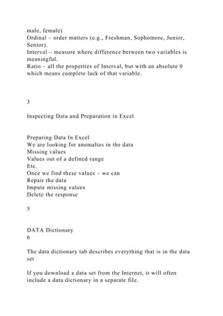
  • 22. Questions? __MACOSX/Big Data Analytics Tools./Final Exam materials/._1 BINS 4352 - Association Analysis.pptx Big Data Analytics Tools./Final Exam materials/2 BINS 4352- Data Preparation.pptx Data Preparation Objectives Provide a perspective on how data may have to be prepared for a given Analytics task Understand the relationship between the data mining technique and the business problem being addressed Gain an understanding of the types of data issues that might be found Understand options when it comes to “fixing” or “addressing” data issues Understand what impact “uncleaned” data may have on the analysis Provide a “practical” and “applied” understanding of statistical concepts Data in Data Mining Data: a collection of facts usually obtained as the result of experiences, observations, or experiments. Data may consist of numbers, words, images, … Data: lowest level of abstraction (from which information and knowledge are derived). Nominal – mutually exclusive, but not order categories (e.g.,
  • 23. male, female) Ordinal – order matters (e.g., Freshman, Sophomore, Junior, Senior). Interval – measure where difference between two variables is meaningful. Ratio – all the properties of Interval, but with an absolute 0 which means complete lack of that variable. 3 Inspecting Data and Preparation in Excel Preparing Data In Excel We are looking for anomalies in the data Missing values Values out of a defined range Etc. Once we find these values – we can Repair the data Impute missing values Delete the response 5 DATA Dictionary 6 The data dictionary tab describes everything that is in the data set If you download a data set from the Internet, it will often include a data dictionary in a separate file.
  • 24. Raw data 7 The raw data is the data as it was collected. There have been no changes/modifications to the data at this point. Highlight Blanks 8 All of the data was selected in the spreadsheet Go to FIND & SELECT in Excel (on the HOME Tab) Select “GO TO SPECIAL” Select “Blanks” Then set the fill color to RED Analyze Row / Columns 9 The raw data is the data as it was collected. There have been no changes/modifications to the data at this point. Count non-blank responses Calculate the frequency of the “expected values” Calculate difference from the means Calculate single answer bias
  • 25. How To Handle Anomalies In The Data Decide what your going to do about the anomalies you found in the data. Filter values Repair the file (impute values) Leave them alone Delete responses Etc. If you are going to “change” data or “delete” data, move the original values to a separate sheet. You are documenting what you did This makes it easier to “undo” your change if you need to. 11 Statistica Data This sheet contains the “cleaned” data that you’re going to load into Statistica for further analysis. The excel manipulation was intended to address the “obvious” problems Graphical Inspection Credit Scoring Data in Statistica Application As we have discussed practically all data will need some preparation More over – that preparation may be slightly different based on the application and the type of analysis that you are doing
  • 26. It is important to have a good understanding of both the data and what you’re trying to accomplish through the data mining process Data preparation Handling missing data and outliers Selecting important variables Sampling Data preparation is specific to BOTH the data set and the task. The preparation method and decisions made during data preparation may change if either change Application For Credit Scoring Data Business Need A financial institution has data about their past customers. These customers are classified as either good or bad credit risks based on their history with the institution. The classification (good/bad) is based on whether or not the loan payment was delinquent and the magnitude of the loss A financial institution needs a way to decide if and how much credit to extend to customers who apply for loans. Business goal: reduce the losses due to bad loans Goals of the data mining process Determine the variables that are best predictors of credit risk Find a high performance predictive model that classifies customers Deploy that model to make decisions on future credit applications Update the model as more data is collected Credit Scoring Data Set We are going to explore the credit scoring data set
  • 27. This data will be used to explore Data preparation Classification Try to keep in mind – this will be a “classification exercise”. It can be applied to different data sets and domains where classification is appropriate Examine the dataDataTypeCredit ratingCategoricalBalance of current accountCategoricalDuration of creditContinuousPayment of previous creditCategoricalPurpose of creditCategoricalAmount of creditContinuousValue of savings CategoricalEmployed by current employerCategoricalInstallment in % of available incomeCategoricalMarital statusCategoricalGenderCategoricalLiving in current household forCategoricalMost valuable assetCategoricalAgeContinuousFurther running creditsCategoricalType of apartmentCategoricalNumber of previous credits at this bankCategoricalOccupationCategoricalTrainTestcategorical Credit Scoring Start by looking at the credit scoring application and the business need Review the variables in the credit risk data set Discuss the next steps for the data mining process Classification Classification can be used to classify a variable with 2 or more
  • 28. groups Find the probability of a particular predicted classification. For example: Loan denied Loan approved Examine The Data Below is the data in Statistica It was opened by FILE-> OPEN Look At Some Histograms Of The Data Histograms Credit rating is the dependent variable – it is the one we want to make predictions for Notice that there have been more than twice as many customers with good credit as compared to bad This may mean that we need to adjust our sample to keep the analysis from being “good” credit biased Histograms Here we have the number of previous credits at the bank 5-6 and 7 or more are relatively small compared to the other categories Hence, we may want to recode the data to have a 5 or more category This is a good general rule of thumb
  • 29. Remaining Variables Remaining Variables Note the majority of customers either have no previous credit or have paid back their previous loans Remaining Variables Remaining Variables Remaining Variables Note: that there have been more than twice as many male customers as female customers Remaining Variables Remaining Variables
  • 30. Age is interesting in that you would expect that customers need to be at least 18 years old to apply for credit, so we need to make sure that is the case in the 15-20 year old group Remaining Variables Remaining Variables Next Steps We have stated the business goals and have data available to do the analysis We have visually inspected the data in order to gain a high-level understanding of the data We still need to do more work here But, we have identified our dependent variable (Credit Risk) and the potential predictor variables We need to continue exploring the data and look at things that we can do to prepare the data for analysis Further Analysis Go to the interactive drill down tool Select the “Drill Variables” Select “Payment of Previous Credits” Drill Down Select “No Previous Credits” Go back to the “Drill down variables” and select “Number of Previous Payments”
  • 31. Select “Brush” Previous payment So here we have an apparent contradiction. We have drilled down to look at customers where the Payment of Previous Credits = no previous credits But, yet the number of previous credits at this bank has values for 2-4, 5-6, and 7 or more? Scatter Plot Matrix A scatter plot matrix can help us look for potential outliers Scatter Plot Matrix We can combine this with the Drill Down and look at scatter plots of all of the continuous variables with respect to those where the Payment of Previous Credits = no previous credits Scatter Plot – Duration Of Credit Vs Amount Of Credit Scatter Plot We can look for outliers here If we know that there is a maximum loan amount, then we can remove those that are greater than that value
  • 32. If we know that there is a maximum duration, we can remove all of those that are greater than that Other Graphical Techniques Box Plots A box plot or boxplot is a convenient way of graphically depicting groups of numerical data through their quartiles. Box plots may also have lines extending vertically from the boxes (whiskers) indicating variability outside the upper and lower quartiles, hence the terms box-and-whisker plot and box- and-whisker diagram. Outliers may be plotted as individual points. Box plots are non-parametric: they display variation in samples of a statistical population without making any assumptions of the underlying statistical distribution. The spacing between the different parts of the box indicate the degree of dispersion (spread) and skewness in the data, and show outliers. There Are Several Variations of Box Plots The “box” : The band inside the box is the second quartile (the median). Statistica gives you the option to make this the “mean” The ends of the “whiskers” can represent several possible alternative values: Min and Max of all of the data Lowest datum still within 1.5 interquartile range (IQR) of the lower quartile, and the highest datum still within 1.5 IQR of the upper quartile (often called the Tukey boxplot) one standard deviation above and below the mean of the data
  • 33. Etc. Box Plot These may seem more “primitive” than a histogram, but they do have some advantages They take up less space – so they are particularly useful in comparing distributions among several groups The number and width of bins can greatly impact the appearance of a histogram Box plots are particularly good at identifying outliers in continuous data Box Plots in Statistica Go to “GRAPHS” and select “Box Plots” Graph Type Box Whiskers Regular (will give you 1 variable per graph) Multiple (will give you 1 graph with all on it” Variables – where you select the variables for analysis Box Plots Leave the defaults for Grouping Intervals Middle point Value – median Style – determines the graphics that show the median in the box
  • 34. Box Plots I have re-selected “Multiple” Graph type I prefer the median be marked with a “Line” Box Plots The graph is fairly crowded – but, I can see outliers that are identified by the small circles. I will re-run this with fewer variables to see if we can see it better Box Plots Now we can more clearly see where the outliers are in the data set. These need to be examined for deletion Next we will look at this in SPSS Marking The Outliers Right clicking on the outliers will pull up a menu where you can tell Statistica to “Mark the Outliers” SPSS – Box Plots The data is loaded into SPSS This can be done by loading the same file we used for Statistica
  • 35. Go to “Graphs” and then to “Legacy Dialogs” and Select “Box Plots” Select “Simple” and “Summaries of separate variables” SPSS – Box Plots Next we select the variables and move them to the “Boxes Represent” area Select “OK” SPSS – Box Plots We see output very similar to Statistica. The outliers are marked with “o” on the graph In SPSS the default is to display the “number” of the response with the outlier Inspecting Outliers In Box Plot We want to be very conservative when identifying responses as “outliers” Count how many “outliers” each respondent has For example, response 188 has 3 outliers, 187 has 4 outliers, and so on. I may delete 1 or 2 responses that have a “large” number of outliers and then rerun the box plot. This will cause things to shift a bit I then iterate until I’m happy with the data. Leaving outliers in the data is fine – this may be a “true”
  • 36. response QUESTIONS? Data CategoricalNumerical NominalOrdinalIntervalRatio Histogram of Credit Rating CreditScoring 19v*1000c Credit Rating = 1000*1*Normal(Location=0.7, Scale=0.4585) bad good Credit Rating 0 100 200 300 400 500 600 700 800 No of obs Histogram of Number of previous credits at this bank CreditScoring 19v*1000c Number of previous credits at this bank = 1000*1*Normal(Location=1.407, Scale=0.5777) one 2- 4 5- 6 7 or more Number of previous credits at this bank 0 100 200 300 400 500 600
  • 37. 700 No of obs Histogram of Balance of Current Account CreditScoring 19v*1000c Balance of Current Account = 1000*1*Normal(Location=2.577, Scale=1.2576) no running account no balance <= $300 >$300 Balance of Current Account 0 50 100 150 200 250 300 350 400 450 No of obs Histogram of Duration of Credit CreditScoring 19v*1000c Duration of Credit = 1000*10*Normal(Location=20.903, Scale=12.0588) -1001020304050607080 Duration of Credit 0 50 100 150 200 250 300 350
  • 38. 400 No of obs Histogram of Payment of Previous Credits CreditScoring 19v*1000c Payment of Previous Credits = 1000*1*Normal(Location=2.545, Scale=1.0831) hesistant problematic running accounts no previous credits no problems with current credits paid back Payment of Previous Credits 0 100 200 300 400 500 600 No of obs Histogram of Purpose of Credit CreditScoring 19v*1000c Purpose of Credit = 1000*1*Normal(Location=2.828, Scale=2.7444) other new car used car furniture television household appliances repair education vacation retraining business Purpose of Credit
  • 39. 0 20 40 60 80 100 120 140 160 180 200 220 240 260 280 300 No of obs Histogram of Amount of Credit CreditScoring 19v*1000c Amount of Credit = 1000*5000*Normal(Location=4579.7472, Scale=3951.8525) -$5,000.00 $0.00 $5,000.00 $10,000.00 $15,000.00 $20,000.00 $25,000.00 $30,000.00 Amount of Credit 0 100 200 300 400 500
  • 40. 600 700 800 No of obs Histogram of Value of Savings CreditScoring 19v*1000c Value of Savings = 1000*1*Normal(Location=2.105, Scale=1.58) no savings <140 140-700 700-1400 >1400 Value of Savings 0 100 200 300 400 500 600 700 No of obs Histogram of Employed by Current Employer for CreditScoring 19v*1000c Employed by Current Employer for = 1000*1*Normal(Location=3.384, Scale=1.2083) unemployed <1 year 1-5 years 5-8 years > 8 years Employed by Current Employer for 0 50 100 150 200 250 300 350 400
  • 41. No of obs Histogram of Installment in % of Available Income CreditScoring 19v*1000c Installment in % of Available Income = 1000*1*Normal(Location=2.973, Scale=1.1187) > 35 25-35 15- 25 < 15 Installment in % of Available Income 0 100 200 300 400 500 No of obs Histogram of Marital Status CreditScoring 19v*1000c Marital Status = 1000*1*Normal(Location=2.682, Scale=0.7081) divorced/living apart divorced/living apart/married single married/widowed Marital Status 0 100 200 300 400 500 600 No of obs Histogram of Gender CreditScoring 19v*1000c Gender = 1000*1*Normal(Location=1.31, Scale=0.4627) male female Gender
  • 42. 0 100 200 300 400 500 600 700 800 No of obs Histogram of Living in Current Household for CreditScoring 19v*1000c Living in Current Household for = 1000*1*Normal(Location=2.845, Scale=1.1037) < 1 year 1-5 years 5-8 years >8 years Living in Current Household for 0 50 100 150 200 250 300 350 400 450 No of obs Histogram of Most Valuable Assets CreditScoring 19v*1000c Most Valuable Assets = 1000*1*Normal(Location=2.358, Scale=1.0502) no assets car life insurance ownership of house or land Most Valuable Assets
  • 43. 0 50 100 150 200 250 300 350 No of obs Histogram of Age CreditScoring 19v*1000c Age = 1000*5*Normal(Location=33.544, Scale=11.3498) 1015 20 253035404550556065707580 Age 0 20 40 60 80 100 120 140 160 180 200 220 240 260 No of obs Histogram of Further running credits CreditScoring 19v*1000c Further running credits = 1000*1*Normal(Location=2.675, Scale=0.7056) at other banks
  • 44. at department store no further running credits Further running credits 0 100 200 300 400 500 600 700 800 900 No of obs Histogram of Type of Apartment CreditScoring 19v*1000c Type of Apartment = 1000*1*Normal(Location=1.928, Scale=0.5302) free rented owned Type of Apartment 0 100 200 300 400 500 600 700 800 No of obs Histogram of Number of previous credits at this bank CreditScoring 19v*1000c Number of previous credits at this bank = 1000*1*Normal(Location=1.407, Scale=0.5777) one 2- 4 5- 6 7 or more Number of previous credits at this bank
  • 45. 0 100 200 300 400 500 600 700 No of obs Histogram of Occupation CreditScoring 19v*1000c Occupation = 1000*1*Normal(Location=2.904, Scale=0.6536) unskilled with no permanant residence unskilled with permanant residence skilled employee executive/self-employed Occupation 0 100 200 300 400 500 600 700 No of obs Histogram for brushing: Number of previous credits at this bank N Total: 1000, Selected: 530 Payment of Previous Credits = no previous credits 050100150200250300350400450500 Number of counts one 2- 4 5- 6 7 or more Number of previous credits at this bank
  • 46. Correlations N Total: 1000, Selected: 1000 Duration of Credit Amount of Credit Age Correlations N Total: 1000, Selected: 530 Payment of Previous Credits = no previous credits Duration of Credit Amount of Credit Age Scatterplot of Amount of Credit against Duration of Credit CreditScoring 19v*1000c Amount of Credit = 298.4367+204.818*x 01020304050607080 Duration of Credit -$2,000.00 $0.00 $2,000.00 $4,000.00 $6,000.00 $8,000.00 $10,000.00 $12,000.00 $14,000.00 $16,000.00 $18,000.00 $20,000.00 $22,000.00 $24,000.00 $26,000.00 $28,000.00 Amount of Credit Box Plot of multiple variables 1-ORIGINAL-FULL-DATASET-WALK-THROUGH 61v*261c Median; Box: 25%-75%; Whisker: Non-Outlier Range
  • 47. Median 25%-75% Non-Outlier Range Outliers Extremes CCSC_1 CCOC_1 CCAC_1 CCAC_6 HCA_5 UCA_4 PEOU_3 PU_4 PP_5 BI_5 PF_4 PIIT_1 0 1 2 3 4 5 6 7 8 Box Plot of multiple variables 1-ORIGINAL-FULL-DATASET-WALK-THROUGH 61v*261c Median; Box: 25%-75%; Whisker: Non-Outlier Range Median 25%-75% Non-Outlier Range Outliers Extremes UCA_1 UCA_3
  • 48. UCA_5 PEOU_1 PEOU_3 PU_1 PU_3 PP_1 PP_3 PP_5 0 1 2 3 4 5 6 7 8 __MACOSX/Big Data Analytics Tools./Final Exam materials/._2 BINS 4352- Data Preparation.pptx Big Data Analytics Tools./Final Exam materials/2 BINS 4352 - Cluster Analysis.pptx Cluster Analysis Cluster Analysis - Review Outline What is it? What is a cluster? How is it different from a decision tree? What is distance and linkage? What is hierarchical clustering?
  • 49. What is scree plot and denogram? What is non-hierarchical clustering (k-means)? How to learn it in detail? 3 Simple Case StudyStudentPhysicsCalculusJoe1520Bill2015Paula2621Jane44 52Jack5045Carlos5738Carla8085Russell9088Eddie9898 4 If we look at the student data on the left, we can easily see a pattern emerging There are natural groupings of students that seem to be apparent in the data. Plotting these on a 2-dimensional scatter plot makes it more visible Similarities And Dissimilarities If we look at the objects in any one of the groupings, they are all very similar to the other objects in that grouping Also, if we look at any one object in a grouping, it is very dissimilar to any object in another grouping This give rise to the notion of: Homogeneous within and Heterogeneous across based on characteristics Clusters
  • 50. These groupings are clusters They represent a “natural grouping of similar objects” based on a collection of input parameters Now, if you add a third or forth dimension (e.g., English, History), then the clusters may change However, the way in which they are constructed is the same Clusters Clusters There is no objective function (i.e., an equation to be optimized given certain constraints with variables that need to be minimized or maximized such as trying to express a business goal in mathematical terms) There is no dependent variable This is sometimes called subjective segmentation The segmentation is developed on its own based on the values of the input variables It is called a unsupervised learning technique. Once the segments are developed They need to be understood You need to decide how you are going to deal with the segments that have emerged How Is This Different From A Decision Tree Decision tree technique requires a clearly defined dependent variable For example, GOOD/BAD credit The technique is based on identifying those variables (characteristics) which are closely associated with the dependent variable.
  • 51. Distances Distances (cont) Paula Bill Joe Jane Jack Carlos Carla Russell Eddie Distance Between 2 Clusters Sometimes called the linkage function: intermediate cluster distance How do you calculate the distance between 2 clusters
  • 53. Single linkage Calculate the distance between each point in one cluster to each point in the neighboring cluster and then find the shortest distance. Complete linkage Similar to single linkage – except we look for the furthest distance Centroid distance Calculate the “center” of each cluster and then calculate the distance between centroids Hierarchical Clustering Used when you have a small number of observations (usually hundreds) You can not use this method for a large dataset because it becomes computationally impractical The way this works is to join objects (cases) together into successively larger clusters using some measure of similarity or distance During the clustering process it shows how the clusters are formed The result of the clustering is the hierarchical tree In SAS this is done by using the “proc cluster” command In Statistica this is called Joining or Tree Clustering Hierarchical Clustering We begin by each case in a cluster by itself In each step we slowly “relax” the criterion which defines
  • 54. “uniqueness” In other words, we lower the threshold by what it means to declare two or more objects within the same cluster As a result we group more and more objects together and each “layer” consists of increasingly dissimilar objects In the last step – all objects are grouped together into a single cluster Scree Plot When we look at a scree plot what we have is the “within cluster variance” Total variance = between variance + within variance The “elbow” in the graph indicates the optimal number of clusters When the number of clusters = 1, the within group variance = total variance Dendogram When the data contain a clear structure in terms of clusters, then its structure is often reflected in the hierarchical tree The result of a successful analysis is that you can detect and interpret the structure by looking at the branches Hierarchical Clustering - Students Everything starts out in a cluster by itself Find the closest objects. Merge those into a cluster. Recalcuate distances (from center of new cluster)
  • 55. Find the closest objects. Merge those into a cluster. Recalcuate distances (from center of new cluster) Joe Bill Paula Jack Jane … K-means Clustering Non-hierarchical Used when you have a large number of observations You decide up front how many clusters you need (k) K-means algorithm Partition objects into k non-empty subsets (randomly) Compute the centroid for each of the clusters Centroid is the center (i.e., mean point of the cluster) This defines the “seed” point for each cluster Assign each object to the cluster with the nearest seed point Go back to step 2 and repeat until the assignment does not change In SAS you do this my using the “proc fastclus” command EM Clustering in Statistica Getting started EM algorithm Uses distributions of (continuous) the data to find the clusters You specify the distribution technique Very similar to K-means clustering
  • 56. First step – hypothesize how many clusters will be in the data With K-means and EM, the optimum number of clusters can be determined with V-fold cross validation Setting Up A Cluster Analysis Go to DATA MINING -> Cluster This will pull up the K-means / EM clustering dialog box Use EM clustering Select all of the variables (Except for Sample) Select Variables And Configure V-fold Validation Select EM algorithm Number of clusters 2 Number of iterations 50 Keep defaults on EM tab – we have limited options here due to all of the variables are categorical On the Validation tab select V-fold cross validation Statistica will search for the optimum number of clusters between 2 and 25 clusters Select “OK”