Big Data Tools MapReduce,Hive and Pig.pdf

MapReduce, Hive and Pig
By :
Sharmila Chidaravalli
Assistant Professor
Department of ISE
Global Academy of Technology

Introduction,
MapReduce Map Tasks,
Reduce Tasks and MapReduce Execution,
Composing MapReduce for Calculations and Algorithms,
Hive,
HiveQL,
Pig.

Hadoop is a software framework for writing distributed applications.
Hadoop processes Big Data (multi-terabyte datasets) in parallel and in a reliable and fault-tolerant way.
MapReduce functions are an integral part of the Hadoop physical organization.
MapReduce is a programming model for the distributed computing environment.
Applications using MapReduce v2, process huge amounts of data, in parallel, on a large number of data
nodes reliably.
The major ecosystem components of Hadoop, are AVRO, Zookeeper, Ambari, HBase, Hive, Pig and
Mahout.
This chapter focuses on details of MapReduce, Hive and Pig programming and their use in Big Data
applications.

Introduction
Big Data architecture design layers

Data Storage Layer:
• Hadoop file system [HDFS] provides the distributed data storage facility.
The data processing layer:
• is the application support layer, while the application layer is the data consumption layer in Big-Data
architecture design.
• Big Data processing layer includes the APIs of Programs such as MapReduce and Spark.
• Data processing layer includes HBase which creates column-family data store using other formats
such as key-value pairs or JSON file.
• HBase stores and processes the columnar data after translating into MapReduce tasks to run in HDFS.

• Data processing layer also includes Hive which creates SQL-like tables.
• Hive stores and processes table data after translating it into MapReduce tasks to run in HDFS.
• Hive creates SQL-like tables in Hive shell.
• Hive uses HiveQL processes queries, ad hoc (unstructured) queries, aggregation functions
and summarizing functions, such as functions to compute maximum, minimum, average of
selected or grouped datasets.
• HiveQL is a restricted form of SQL.

• The support layer also includes Pig.
• Pig is a data-flow language and an execution framework.
• Pig enables the usage of relational algebra in HDFS.
• MapReduce is the processing framework and YARN is the resource managing framework

Key terms
MapReduce programming model refers to a programming paradigm for processing Big Data
sets with a parallel and distributed environment using map and reduce tasks.
YARN refers to provisioning of running and scheduling parallel programs for map and reduce
tasks and allocating parallel processing resources for computing sub-tasks running in parallel at
the Hadoop for a user application.
Script refers to a small program (codes up to few thousand lines of code) used for purposes such
as query processing, text processing, or refers to a small code written in a dynamic high-level
general-purpose language, such as Python or PERL.

SQL-like scripting language:
means a language for writing script that processes queries similar to SQL. SQL lets us:
(i) write structured queries for processing in DBMS,
(ii) create and modify schema, and control the data access,
(iii) create client for sending query scripts, and create and manage server databases, and
(iv) view, query and change (update, insert or append or delete) databases.

NoSQL DBs refers to DBs with no prior fixed schema, schema-less models, and databases which
possess increasing flexibility for data manipulation.
NoSQL data model
Relaxation in one or more of the ACID properties (Atomicity, Consistence, Isolation and Durability) of
the database.
A theorem known as CAP (Consistency, Availability and Partitions) states that out of three properties,
at least two must be present.
NoSQL relies upon another model known as the BASE model.
BASE model has three principles: Basic availability (the availability of data even in the presence of
multiple failures), Soft state (data consistency is the developer's problem and should not be handled by
the database), Eventual consistency (when no new changes occur on existing data, eventually all
accesses to that data will return the last updated value).

Data-architecture patterns refer to formats used in NoSQL DBs. The examples are Key-Value Data
Stores, Object Data Stores, Column family Big Data Stores, Tabular Data Stores and Document Stores,
Graph Data Store.
Key-Value Data Store refers to a simplest way to implement a schema-less database. A string called key
maps to values in a large data string hence storage easily scales up and data retrievals are fast.
Object Data Store refers to a repository which stores the
(i) objects (such as files, images, documents, folders and business reports),
(ii) system metadata which provides information such as filename, creation_date, last_modified,
language_used (such as Java, C, C#, C++, Smalltalk, Python), access_permissions, supported Query
languages, and
(iii) Custom metadata which provides information such as subject, category and sharing permission.

Tabular Data Store refers to table, column-family or BigTable like Data Store.
Column family Big Data store refers to a storage in logical groups of column families. The storage
may be similar to columns of sparse matrix. They use a pair of row and column keys to access the
column fields.
BigTable Data Store is a popular column-family based Data Store. Row key, column key and
timestamp uniquely identify a value. Google BigTable, HBase and Cassandra DBs use the BigTable
Data Store model.
Document Store means a NoSQL DB which stores hierarchical information in a single unit called
document. Document stores data in nested hierarchies; for example in XML document object model,
JSON formats data model.

Tuple means an ordered list of elements. Tuples implement the records.
Collection means a well-defined collection of distinct objects in a set, the objects of a set are called
elements. A collection is similar to a table of RDBMS.
A collection in a database also refers to storage of a number of documents.
A collection may store documents which do not have the same fields.
Thus, documents in the collection are schema-less. Thus, it is possible to store documents of varying
structures in a collection.
Aggregate refers to collection of data sets in the key value, column family or BigTable data stores which
usually require sequential processing.
Aggregation function refers to a function to find counts, sum, maximum, minimum, other statistical or
mathematical function using a collection of datasets, such as column or column-family.

Natural join is where two tables join based on all common columns. Both the tables must have
the same column name and the data type.
Inner join is the default natural join. It refers to two tables that join based on common columns
mentioned using the ON clause. Inner Join returns all rows from both tables if the columns
match.
Node refers to a place for storing data, data block or read or write computations.
Data center in a DB refers to a collection of related nodes. Many nodes form a data center or
rack.
Cluster refers to a collection of many nodes.
Keyspace means a namespace to group multiple column families or in general name given to
group of tables.

Indexing to a field means providing reference to a field in a document of collections.
Indexing is used to query and perform operations on that document.
A DB creates an index on the _id field of every collection
Projection refers to a unary operation (single input or operand) written as
Projection returns a set obtained by selecting only the n attributes.

Mapreduce Map Tasks, Reduce Tasks and Mapreduce Execution
Big data processing employs the MapReduce programming model.
A Job means a MapReduce program.
Each job consists of several smaller units, called MapReduce tasks.
A software execution framework in MapReduce programming defines the parallel tasks.
MapReduce Programming Model

The model defines two important tasks, namely Map and Reduce.
Map takes input data set as pieces of data and maps them on various nodes for parallel
processing.
The reduce task, which takes the output from the maps as an input and combines those data
pieces into a smaller set of data.
A reduce task always run after the map task (s).
Many real-world situations are expressible using this model.
This Model describes the essence of MapReduce programming where the programs written are
automatically parallelize and execute on a large cluster.

MapReduce Programming Model
• Parallel processing of large data sets, based on a YARN-based system
• Each job consisting of number of Map and Reduce tasks, running in parallel
• Java Programming Framework
• Input Data flow to Map Task
• MapTask maps, shuffles, sorts and other operations
• Sends output to Reduce Task
• Reduce task produces results using combiner, aggregation, count or other reduce
functions
• Output of Reducer Tasks flows to ─ Application Support APIs and Application

Mapreduce Process On Client Submitting a Job

A user application specifies locations of the input/output data and translates into map and
reduce functions.
JobTracker and Task Tracker MapReduce consists of a single master JobTracker and
one slave TaskTracker per cluster node.
The Hadoop job client then submits the job (jar/executable etc.) and configuration to the
JobTracker, which then takes the responsibility of distributing the software/configuration to the
slaves by scheduling tasks, monitoring them, and provides status and diagnostic information to
the job-client.
The master is responsible (JobTracker) for scheduling the component tasks in a job onto
the slaves, monitoring them and re-executing the failed tasks. The slaves execute the tasks as
directed by the master.

The data for a MapReduce task is typically residing in the HDFS in the form of files.
The files may be line-based log files, binary format file, multi-line input records, or
something else entirely different.
The data in files may be in the form of key value pairs, documents, Tabular data, line-
based log files, binary format file, multi-line input records.
These input files are practically very large, hundreds of terabytes or even more than it.
The MapReduce framework operates entirely on key, value-pairs. The framework
views the input to the task as a set of (key, value) pairs and produces a set of (key,
value) pairs as the output of the task, possibly of different types.

Map-Tasks
Implements a map (), which runs user application codes for each key-value pair (k1, v1).
Key k1─ a set of keys.
k1 maps to a group of data values v1.
Values v1─ a large string which is read from the input file(s)
The output of map() would be zero (when no values are found) or intermediate key-value pairs (k2, v2).
The value v2 is the information that is later used at reducer for the transformation operation using
aggregation or other reducing functions.

Reduce task refers to a task which takes the output v2 from the map as an input and combines those data
pieces into a smaller set of data using a combiner. The reduce task is always performed after the map
task.
The Mapper performs a function on individual values in a dataset irrespective of the data size of the
input. That means that the Mapper works on a single data set.
Map-Tasks
Logical view of functioning of map().

Hadoop Java API includes Mapper class. An abstract function map() is present in the Mapper class.
Any specific Mapper implementation should be a subclass of this class and overrides the abstract function, map
().
The Sample Code for Mapper Class
public clase SampleMapper extends Mapper<kl, Vl, k2, v2>
{
void map (kl key, Vl value, Context context) throwe IOException, InterruptedException
{ ..}
}
Individual Mappers do not communicate with each other.
Map-Tasks

Number of Maps
The number of maps depends on the size of the input files, i.e., the total number of blocks of the
input files.
If the input files are of 1TB in size and the block size is 128 MB, there will be 8192 maps.
The number of map task Nmap can be explicitly set by using setNumMapTasks(int).
Suggested number is nearly 10-100 maps per node.
Nmap can be set even higher.
Map-Tasks

Key-Value Pair
Each phase (Map phase and Reduce phase) of MapReduce has key-value pairs as input and output.
Data should be first converted into key-value pairs before it is passed to the Mapper, as the Mapper only understands
key-value pairs of data.
Key-value pairs in Hadoop MapReduce are generated as follows:
InputSplit –
Defines a logical representation of data and presents a Split data for processing at individual map().
RecordReader –
Communicates with the InputSplit and converts the Split into records which are in the form of key-value
pairs in a format suitable for reading by the Mapper.
RecordReader uses TextlnputFormat by default for converting data into key-value pairs.
RecordReader communicates with the InputSplit until the file is read.
Generation of a key-value pair in MapReduce depends on the dataset and the required output.
Also, the functions use the key-value pairs at four places: map() input, map() output, reduce() input and reduce()
output.

Grouping by Key
When a map task completes, Shuffle process aggregates (combines) all the Mapper outputs
by grouping the key-values of the Mapper output, and the value v2 append in a list of values.
A "Group By" operation on intermediate keys creates v2.
Shuffle and Sorting Phase
All pairs with the same group key (k2) collect and group together, creating one group for each key.
Shuffle output format will be a List of <k2, List (v2)>. Thus, a different subset of the intermediate key
space assigns to each reduce node.
These subsets of the intermediate keys (known as "partitions") are inputs to the reduce tasks.
Each reduce task is responsible for reducing the values associated with partitions. HDFS sorts the
partitions on a single node automatically before they input to the Reducer.

Partitioning
 The Partitioner does the partitioning. The partitions are the semi-mappers in MapReduce.
 Partitioner is an optional class. MapReduce driver class can specify the Partitioner.
 A partition processes the output of map tasks before submitting it to Reducer tasks.
 Partitioner function executes on each machine that performs a map task.
 Partitioner is an optimization in MapReduce that allows local partitioning before reduce-task
phase.
 The same codes implement the Partitioner, Combiner as well as reduce() functions.
 Functions for Partitioner and sorting functions are at the mapping node.
 The main function of a Partitioner is to split the map output records with the same key.

Combiners
Combiners are semi-reducers in MapReduce. Combiner is an optional class. MapReduce driver class
can specify the combiner.
The combiner() executes on each machine that performs a map task. Combiners optimize MapReduce
task that locally aggregates before the shuffle and sort phase.
The same codes implement both the combiner and the reduce functions, combiner() on map node and
reducer() on reducer node.
The main function of a Combiner is to consolidate the map output records with the same key.
The output (key-value collection) of the combiner transfers over the network to the Reducer task as
input.
This limits the volume of data transfer between map and reduce tasks, and thus reduces the cost of data
transfer across the network. Combiners use grouping by key for carrying out this function.

Combiners
The combiner works as follows:
 It does not have its own interface and it must implement the interface at
reduce().
 It operates on each map output key. It must have the same input and output
key-value types as the Reducer class.
 It can produce summary information from a large dataset because it
replaces the original Map output with fewer records or smaller records.

Reduced Tasks
Java API at Hadoop includes Reducer class. An abstract function, reduce() is in the Reducer.
• Any specific Reducer implementation should be subclass of this class and override the abstract reduce().
• Reduce task implements reduce() that takes the Mapper output (which shuffles and sorts), which is
grouped by key-values (k2, v2) and applies it in parallel to each group.
• Intermediate pairs are at input of each Reducer in order after sorting using the key.
• Reduce function iterates over the list of values associated with a key and produces outputs such as
aggregations and statistics.
• The reduce function sends output zero or another set of key-value pairs (k3, v3) to the final the output
file. Reduce: {(k2, list (v2) -> list (k3, v3)}
Sample code for Reducer Class
public class ExarrpleReducer extends Reducer<k2, v2, k3, v3>
void reduce (k2 key, Iterable<V2> values, Context context) throws IOBxception,
InterruptedBxception
{ ... } }

Details of Map Reduce processing Steps.

Phases of MapReduce – How Hadoop MapReduce Works
Phases of MapReduce job execution like Input Files, InputFormat, InputSplits, RecordReader, Mapper, Combiner,
Partitioner, Shuffling, and Sorting, Reducer, RecordWriter, and OutputFormat

MapReduce Implementation Phases : Example
Let us assume we have the following input text file named input.txt for MapReduce.

Record Reader
This is the first phase of MapReduce where the Record Reader reads every line from the input
text file as text and yields output as key-value pairs.
Input − Line by line text from the input file.
Output − Forms the key-value pairs. The following is the set of expected key-value pairs.

Map Phase
The Map phase takes input from the Record Reader, processes it, and produces the output as
another set of key-value pairs.
Input − The following key-value pair is the input taken from the Record Reader.
Output − The expected output is as follows

Combiner Phase
The Combiner phase takes each key-value pair from the Map phase, processes it, and
produces the output as key-value collection pairs.
Input − The following key-value pair is the input taken from the Map phase.
Output − The expected output is as follows

The Reducer phase takes each key-value collection pair from the Combiner phase, processes it, and passes
the output as key-value pairs. Note that the Combiner functionality is same as the Reducer.
Input − The following key-value pair is the input taken from the Combiner phase.
Output − The expected output from the Reducer phase is as follows
Reducer Phase

Record Writer
This is the last phase of MapReduce where the Record Writer writes every key-value pair from the
Reducer phase and sends the output as text.
Input − Each key-value pair from the Reducer phase along with the Output format.
Output − It gives you the key-value pairs in text format. Following is the expected output.

Copying with Node Failure
The primary way using which Hadoop achieves fault tolerance is through restarting the tasks.
• Each task nodes (TaskTracker) regularly communicates with the master node, JobTracker. If a
TaskTracker fails to communicate with the JobTracker for a pre-defined period (by default, it is set
to 10 minutes), a task node failure by the JobTracker is assumed.
• The JobTracker knows which map and reduce tasks were assigned to each TaskTracker.
• If the job is currently in the mapping phase, then another TaskTracker will be assigned to re-execute
all map tasks previously run by the failed TaskTracker.
• If the job is in the reducing phase, then another TaskTracker will re-execute all reduce tasks that
were in progress on the failed TaskTracker.
• Once reduce tasks are completed, the output writes back to the HDFS. Thus, if a TaskTracker has
already completed nine out of ten reduce tasks assigned to it, only the tenth task must execute at a
different node.

The failure of JobTracker (if only one master node) can bring the entire process down; Master handles
other failures, and the MapReduce job eventually completes. When the Master compute-node at which
the JobTracker is executing fails, then the entire MapReduce job must restart.
Following points summarize the coping mechanism with distinct Node Failures:
• Map TaskTracker failure:
Map tasks completed or in-progress at TaskTracker, are reset to idle on failure
Reduce TaskTracker gets a notice when a task is rescheduled on another TaskTracker
• Reduce TaskTracker failure:
Only in-progress tasks are reset to idle
• Master JobTracker failure:
Map-Reduce task aborts and notifies the client (in case of one master node).
Copying with Node Failure

Composing Mapreduce For Calculations And Algorithms
MapReduce program composition in
counting and summing,
algorithms for relational algebraic operations,
projections, unions, intersections, natural joins,
grouping and aggregation,
matrix multiplication and other computations.

Composing Map-Reduce for Calculations
Counting and Summing
Count /Sum the number of alerts or messages generated during a specific
maintenance activity of vehicles need counting for a month.
 The pseudocode using emit() in the map() of Mapper class. Mapper emits 1 for each
message generated.
 The reducer goes through the list of ls and sums them. Counting is used in the data
querying application.
 For example, count of messages generated, word count in a file, number of cars sold, and
analysis of the logs, such as number of tweets per month. Application is also in business
analytics field.

Counting and Summing

Sorting
 MapReduce execution steps, i.e., dataflow, splitting, partitioning and sorting on a map
node and reduce on a reducer node.
 Mappers just emit all items as values associated with the sorting keys which assemble as
a function of items.
 Reducers combine all emitted parts into a final list.

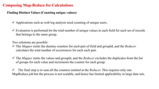
Finding Distinct Values (Counting unique values)
 Applications such as web log analysis need counting of unique users.
 Evaluation is performed for the total number of unique values in each field for each set of records
that belongs to the same group.
Two solutions are possible:
 The Mapper emits the dummy counters for each pair of field and groupld, and the Reducer
calculates the total number of occurrences for each such pair.
 The Mapper emits the values and groupld, and the Reducer excludes the duplicates from the list
of groups for each value and increments the counter for each group.
 The final step is to sum all the counters emitted at the Reducer. This requires only one
MapReduce job but the process is not scalable, and hence has limited applicability in large data sets.

Filtering or Parsing
 Filtering or parsing collects only those items which satisfy some condition or
transform each item into some other representation.
 Filtering/parsing include tasks such as text parsing, value extraction and conversion
from one format to another.
 Examples of applications of filtering are found in data validation, log analysis and
querying of datasets.
 Mapper takes items one by one and accepts only those items which satisfy the
conditions and emit the accepted items or their transformed versions.
 Reducer obtains all the emitted items, saves them into a list and outputs to the
application.

Distributed Tasks Execution
 Large computations divide into multiple partitions and combine the results from all
partitions for the final result.
 Examples of distributed running of tasks are physical and engineering simulations,
numerical analysis and performance testing.
 Mapper takes a specification as input data, performs corresponding computations and
emits results. Reducer combines all emitted parts into the final result.

Graph Processing using Iterative Message Passing
 Graph is a network of entities and relationships between them. A node corresponds to an entity. An edge joining
two nodes corresponds to a relationship.
 Path traversal method processes a graph. Traversal from one node to the next generates a result which passes as a
message to the next traversal between the two nodes. Cyclic path traversal uses iterative message passing.
 A set of nodes stores the data and codes at a network. Each node contains a list of neighboring node IDs.
MapReduce jobs execute iteratively. Each node in an iteration sends messages to its neighbors.
 Each neighbor updates its state based on the received messages. Iterations terminate on some conditions, such as
completion of fixed maximal number of iterations or specified time to live or negligible changes in states between
two consecutive iterations.
 Mapper emits the messages for each node using the ID of the adjacent node as a key. All messages thus group by
the incoming node. Reducer computes the state again and rewrites a node new state.

Cross Correlation
Cross-correlation involves calculation using number of tuples where the items co-occur in a set of tuples
of items. If the total number of items is N, then the total number of values= N x N. Cross correlation is
used in text analytics. (Assume that items are words and tuples are sentences). Another application is in
market-analysis (for example, to enumerate, the customers who buy item x tend to also buy y).
If N x N is a small number, such that the matrix can fit in the memory of a single machine, then
implementation is straightforward.
Two solutions for finding cross correlations are:
 The Mapper emits all pairs and dummy counters, and the Reducer sums these counters.
 The benefit from using combiners is little, as it is likely that all pairs are distinct. The accumulation
does not use in-memory computations as N is very large.
 The Mapper groups the data by the first item in each pair and maintains an associative array
("stripe") where counters for all adjacent items accumulate.
 The Reducer receives all stripes for the leading item, merges them and emits the same result as in the
pairs approach.

The grouping
 Generates fewer intermediate keys. Hence, the framework has less sorting todo.
 Greatly benefits from the use of combiners.
 In-memory accumulation possible.
 Enables complex implementations.
 Results in general, faster computations using stripes than "pairs".

Relational – Algebra Operations
Selection
Consider the attribute names (ACVM_ID, Date, chocolate_flavour, daily_sales).
Consider relation
R = {(524, 12122017, KitKat, 82),
(524, 12122017, Oreo, 72),
(525 2122017, KitKat, 82),
(525, 12122017, Oreo, 72),
(526, 12122017, KitKat, 82),
(526, 12122017, Oreo, 72)}.
Selection ACVM_ID <= 525 (R)
selects the subset R= {(524, 12122017, KitKat, 82),
(524, 12122017, Oreo, 72),
(525, 12122017, KitKat, 82),
(525, 12122017, Oreo, 72)}.
Selection chocolate_flavour= Oreo
selects the subset R= {(524, 12122017, Oreo, 72),
(525, 12122017, Oreo, 72),
(526, 12122017, Oreo, 72)}.
The Mapper
calls test() for each tuple in a row.
When test satisfies the selection criterion then
emits the tuple.
The Reducer
transfers the received input tuple as the output.

Projection
Consider attribute names (ACVM_ID, Date, chocolate_flavour, daily_sales).
Consider relation
R = {(524, 12122017, KitKat, 82),
(524, 12122017, Oreo, 72)}.
Projection II ACVM_m (R)
selects the subset {(524)}.
Projection, II chocolate_flavour, 0.5* daily_sales (R)
selects the subset
{(KitKat, 0.5x82), (Oreo, 0.5 X 72)}
The Mapper
calls test() for each tuple in a row. When the test satisfies, the
predicate then emits the tuple (same as in selection).
The Reducer
transfers the received input tuples after eliminating the possible
duplicates. Such operations are used in analytics

Union
Consider,
Rl = {(524, 12122017, KitKat, 82), (524, 12122017, Oreo, 72)}
R2 = {(525, 12122017, KitKat, 82), (525, 12122017, Oreo, 72)}
R3 = {(526, 12122017, KitKat, 82), (526, 12122017, Oreo, 72)}
Result of Union operation between Rl and R3 is:
Rl U R3 =
{(524, 12122017, KitKat, 82),
(524, 12122017, Oreo, 72),
(526, 12122017, KitKat, 82),
(526, 12122017, Oreo, 72)}
The Mapper
executes all tuples of two sets for union and emits all the resultant tuples.
The Reducer
class object transfers the received input tuples after eliminating the possible
duplicates.

Intersection
Consider,
Rl = {(524, 12122017, Oreo, 72)}
R2 = {(525, 12122017, KitKat, 82)}
R3 = {(526, 12122017, KitKat, 82), (526, 12122017, Oreo, 72)}
Result of Intersection operation between Rl and R3 are
Rl n R3 = {(12122011, Oreo)}
The Mapper
executes all tuples of two sets for intersection and emits all the resultant tuples.
The Reducer
transfers only tuples that occurred twice. This is possible only when tuple includes primary
key and can occur once in a set. Thus, both the sets contain this tuple.

Difference
Consider:
Rl = {(12122017, KitKat, 82), (12122017, Oreo, 72)}
R3 = {(12122017, KitKat, 82), (12122017, Oreo, 25)}
Difference means the tuple elements are not present in the second relation.
Therefore, difference
set_l is Rl - R3 = (12122017, Oreo, 72)
set_2 is R3 - Rl = (12122017, Oreo, 25).
The Mapper
emits all the tuples and tag. A tag is the name of the set (say, set_l or set_2 to which a
tuple belongs to).
The Reducer
transfers only tuples that belong to set_l.

Natural Join
Consider two relations Rl and R2 for tuples a, b and c.
Natural Join computes for Rl (a, b) with R2 (b, c).
Natural Join is R (a, b, c).
Tuples b joins as one in a Natural Join.
The Mapper
emits the key-value pair (b, (Rl, a)) for each tuple (a, b) of Rl, similarly emits (b, (R2, c)) for
each tuple (b, c) of R2.
The Mapper is mapping both with Key for b.
The Reducer
transfers all pairs consisting of one with first component Rl and the other with first component
R2, say (Rl, a) and (R2, c).
The output from the key and value list is a sequence of key-value pairs. The key is of no use and
is irrelevant. Each value is one of the triples (a, b, c) such that (Rl, a) and (R2, c) are present in
the input list of values.

Grouping and Aggregation by MapReduce
Grouping means operation on the tuples by the value of some of their attributes after applying the
aggregate function independently to each attribute.
A Grouping operation denotes by <grouping attributes> j <function-list> (R).
Aggregate functions are count(), sum(), avg(), min() and max().
Assume
R= {
(524, 12122017, KitKat, 82),
(524, 12122017, Oreo, 72),
(525,12122017, KitKat, 82),
(525, 12122017, Oreo, 72),
(526, 12122017, KitKat, 82),
(526, 12122017, Oreo, 72)}.
Chocolate_flavour i count ACVM_ID, sum (daily_sales (chocolate_flavour)) will give the output
(524, KitKat, sale_month), (525, KitKat, sale_month), .... and (524, Oreo, sale_month), (525, Oreo,
sale_month), .... for all ACVM_IDs.
The Mapper : finds the values from each tuple for grouping and aggregates them.
The Reducer : receives the already grouped values in input for aggregation.

Matrix Multiplication With 1 MapReduce Step
MapReduce is a technique in which a huge program is subdivided into small tasks and run
parallelly to make computation faster, save time, and mostly used in distributed systems.
It has 2 important parts:
Mapper: It takes raw data input and organizes into key, value pairs. For example, In a dictionary,
you search for the word “Data” and its associated meaning is “facts and statistics collected together
for reference or analysis”. Here the Key is Data and the Value associated with is facts and statistics
collected together for reference or analysis.
Reducer: It is responsible for processing data in parallel and produce final output.

Mapper for Matrix A (k, v)=((i, k), (A, j, Aij)) for all k
Mapper for Matrix B (k, v)=((i, k), (B, j, Bjk)) for all i
Mapper
Reducer(k, v)=(i, k)=>Make sorted Alist and Blist
(i, k) => Summation (Aij * Bjk)) for j
Output =>((i, k), sum)
Reducer

Let us consider the matrix multiplication example to visualize MapReduce. Consider the following matrix:
Here
Matrix A is a 2×2 matrix which means the number of rows(i)=2 and the number of columns(j)=2.
Matrix B is also a 2×2 matrix where number of rows(j)=2 and number of columns(k)=2.
Each cell of the matrix is labelled as Aij and Bij.
Ex. element 3 in matrix A is called A21 i.e. 2nd-row 1st column.
Now One step matrix multiplication has 1 mapper and 1 reducer.

Therefore computing the mapper for Matrix A: Matrix A (k, v)=((i, k), (A, j, Aij)) for all k
# k, i, j computes the number of times it occurs.
# Here all are 2, therefore when k=1, i can have #2 values 1 & 2, each case
can have 2 further values of j=1 and j=2.
Substituting all values # in formula
k=1
i=1 j=1 ((1, 1), (A, 1, 1)) j=2 ((1, 1), (A, 2, 2))
i=2 j=1 ((2, 1), (A, 1, 3)) j=2 ((2, 1), (A, 2, 4))
k=2
i=1 j=1 ((1, 2), (A, 1, 1)) j=2 ((1, 2), (A, 2, 2))
i=2 j=1 ((2, 2), (A, 1, 3)) j=2 ((2, 2), (A, 2, 4))

Computing the mapper for Matrix B :Mapper for Matrix B (k, v)=((i, k), (B, j, Bjk)) for all i
i=1
j=1 k=1 ((1, 1), (B, 1, 5)) k=2 ((1, 2), (B, 1, 6))
j=2 k=1 ((1, 1), (B, 2, 7)) k=2 ((1, 2), (B, 2, 8))
i=2
j=1 k=1 ((2, 1), (B, 1, 5)) k=2 ((2, 2), (B, 1, 6))
j=2 k=1 ((2, 1), (B, 2, 7)) k=2 ((2, 2), (B, 2, 8))

Computing the reducer:
We can observe from Mapper computation that 4 pairs are common (1, 1), (1, 2), # (2, 1) and (2, 2) .Make a list
separate for Matrix A & B with adjoining values taken from Mapper step above:
(1, 1) => Alist ={(A, 1, 1), (A, 2, 2)}
Blist ={(B, 1, 5), (B, 2, 7)}
Now Aij x Bjk: [(1*5) + (2*7)] =19 -------(i)
(1, 2) => Alist ={(A, 1, 1), (A, 2, 2)}
Blist ={(B, 1, 6), (B, 2, 8)}
Now Aij x Bjk: [(1*6) + (2*8)] =22 -------(ii)
(2, 1) => Alist ={(A, 1, 3), (A, 2, 4)}
Blist ={(B, 1, 5), (B, 2, 7)}
Now Aij x Bjk: [(3*5) + (4*7)] =43 -------(iii)
(2, 2) => Alist ={(A, 1, 3), (A, 2, 4)}
Blist ={(B, 1, 6), (B, 2, 8)}
Now Aij x Bjk: [(3*6) + (4*8)] =50 -------(iv)
From (i), (ii), (iii) and (iv)
we conclude that
((1, 1), 19)
((1, 2), 22)
((2, 1), 43)
((2, 2), 50)
Therefore the Final Matrix is:

HIVE
Hive was created by Facebook.
Hive is a data warehousing tool and is also a data store on the top of Hadoop.
Enterprises uses a data warehouse as large data repositories that are designed to enable the
Searching, managing, and analyzing the data.
Hive processes structured data, integrates well heterogeneous sources.
Additionally, also manages the volumes of data.

Hive Characteristics
 Has the capability to translate queries into MapReduce jobs. This makes Hive
scalable, able to handle data warehouse applications, and therefore, suitable for the
analysis of static data of an extremely large size, where the fast response-time is
not a criterion.
 Supports web interfaces as well. Application APIs as well as web-browser
clients, can access the Hive DB server.
 Provides an SQL dialect (Hive Query Language, abbreviated HiveQL or HQL).
Results of HiveQL Query and the data load in the tables which store at the Hadoop
cluster at HDFS.

HIVE Limitations
1. Not a full database. Main disadvantage is that Hive does not provide update, alter
and deletion of records in the database.
2. Not developed for unstructured data.
3. Not designed for real-time queries.
4. Performs the partition always from the last column.

HIVE Architecture
Components of Hive architecture are:
 Hive Server (Thrift) - An optional service that allows a remote client to submit requests to Hive
and retrieve results. Requests can use a variety of programming languages.
 Thrift Server exposes a very simple client API to execute HiveQL statements.
 Hive CLI (Command Line Interface) - Popular interface to interact with Hive. Hive runs in local
mode that uses local storage when running the CLI on a Hadoop cluster instead of HDFS.
 Web Interface - Hive can be accessed using a web browser as well. This requires a HWI Server
running on some designated code. The URL http:// hadoop:<port no.> / hwi command can be used
to access Hive through the web.
 Metastore - It is the system catalog. All other components of Hive interact with the Metastore. It
stores the schema or metadata of tables, databases, columns in a table, their data types and HDFS
mapping.
 Hive Driver - It manages the life cycle of a HiveQL statement during compilation, optimization and
execution.

Comparison with RDBMS (Traditional Database)

Hive Data Types and File Formats
Hive defines various primitive, complex, string, date/time, collection data types and file formats for
handling and storing different data formats.
The following Table gives primitive, string, date/time and complex Hive data types and their
descriptions.

Hive has three Collection data types

HIVE file formats and their descriptions

Hive Integration and Workflow Steps
Hive integrates with the MapReduce and HDFS. Figure below shows the dataflow sequences and workflow
steps between Hive and Hadoop.

Step 1
Execute Query: Hive interface (CLI or Web Interface) sends a query to Database Driver to execute the query.
Step 2
Get Plan: Driver sends the query to query compiler that parses the query to check the syntax and query plan or
the requirement of the query.
Step 3
Get Metadata: Compiler sends metadata request to Metastore (of any database, such as MySQL).
Step 4
Send Metadata: Metastore sends metadata as a response to compiler.
Sep 5
Send Plan: Compiler checks the requirement and resends the plan to driver. The parsing and compiling of the
query is complete at this place.
Sep 6
Execute Plan: Driver sends the execute plan to execution engine.

Step 7
Execute Job: Internally, the process of execution job is a MapReduce job. The execution engine
sends the job to JobTracker, which is in Name node and it assigns this job to TaskTracker, which is
in Data node. Then , the query executes the job.
Step 8
Metadata Operations: Meanwhile the execution engine can execute the metadata operations with
Metastore.
Step 9
Fetch Result: Execution engine receives the results from Data nodes.
Step 10
Send Results: Execution engine sends the result to Driver.
Step 11
Send Results: Driver sends the results to Hive Interfaces.

Hive Built-in Functions
Return Type Syntax Description
BIGINT round(double a) Returns the rounded BIGINT (8 Byte
integer) value of the 8 Byte double-
precision floating point number a
BIGINT floor(double a) Returns the maximum BIGINT value
that is equal to or less than the
double.
BIGINT ceil(double a) Returns the minimum BIGINT value
that is equal to or greater than the
double.
double rand(), rand(int seed) Returns a random number (double)
that distributes uniformly from O to 1
and that changes in each row. Integer
seed ensured that random number
sequence is deterministic.
string concate(string strl, string str2, ...) Returns the string resulting from
concatenating strl with str2,

string substr(string str, int start) Returns the substring of str starting
from a start position till the end of
string str
string substr(string str, int start, int length) Returns the substring of str starting
from the start position with the given
length.
string upper(string str), ucase (string str) Returns the string resulting from
converting all characters of str to
upper case.
string lower(string str), lcase(string str) Returns the string resulting from
converting all characters of str to
lower case.
string trim(string str) Returns the string resulting from
trimming spaces from both ends. trim
('12A34 56') returns '12A3456'

string ltrim(string str); rtrim(string str) Returns the string resulting from trimming
spaces (only one end, left or right hand side
or right-handside spaces trimmed).
ltrim('12A34 56') returns '12A3456' and
rtrim(' 12A34 56 ') returns '12A3456'.
string rtrim(string str) Returns the string resulting from trimming
spaces from the end (right hand side) of str.
int year(string date) Returns the year part of a date or a
timestamp string.
int month(string date) Returns the month part of a date or a
timestamp string .
int day(string date) Returns the day part of a date or a
timestamp string.

 Hive Query Language (abbreviated HiveQL) is for querying the large datasets which reside in
the HDFS environment.
 HiveQL script commands enable data definition, data manipulation and query processing.
 HiveQL supports a large base of SQL users who are acquainted with SQL to extract information
from data warehouses.
Hive Query Language
HiveQL Process
Engine
HiveQL is similar to SQL for querying on schema information at the
Metastore. It is one of the replacements of traditional approach for
MapReduce program . Instead of writing MapReduce program in
Java, we can write a query for MapReduce job and process it.
Execution Engine The bridge between HiveQL process Engine and MapReduce is
Hive Execution Engine. Execution engine processes the query and
generates results same as MapReduce results. It uses the flavor of
MapReduce.

HiveQL Data Definition Language (DDL)
HiveQL database commands for data definition for DBs and Tables are
CREATE DATABASE,
SHOW DATABASE (list of all DBs),
CREATE SCHEMA,
CREATE TABLE.

Create Database Statement
Create Database is a statement used to create a database in Hive. A database in Hive is a namespace or a
collection of tables. The syntax for this statement is as follows:
CREATE DATABASE|SCHEMA [IF NOT EXISTS] <database name>
Here, IF NOT EXISTS is an optional clause, which notifies the user that a database with the same name
already exists. We can use SCHEMA in place of DATABASE in this command. The following query is
executed to create a database named userdb:
hive> CREATE DATABASE [IF NOT EXISTS] userdb;
hive> SHOW DATABASES;
default
userdb

Drop Database Statement
Drop Database is a statement that drops all the tables and deletes the database. Its syntax is as follows:
DROP DATABASE StatementDROP (DATABASE|SCHEMA) [IF EXISTS] database_name
[RESTRICT|CASCADE];
The following queries are used to drop a database. Let us assume that the database name is userdb.
hive> DROP DATABASE IF EXISTS userdb;

Create Table Statement
Create Table is a statement used to create a table in Hive.
The syntax and example are as follows:
CREATE [TEMPORARY] [EXTERNAL] TABLE [IF NOT EXISTS] [db_name.] table_name
[(col_name data_type [COMMENT col_comment], ...)]
[COMMENT table_comment]
[ROW FORMAT row_format]
[STORED AS file_format]
If you add the option IF NOT EXISTS, Hive ignores the statement in case the table already exists.

Sr.No Field Name Data Type
1 Eid int
2 Name String
3 Salary Float
4 Designation string
Example
Let us assume you need to create a table named employee using CREATE TABLE statement.
The following table lists the fields and their data types in employee table:
The following query creates a table named employee using the above data.
hive> CREATE TABLE IF NOT EXISTS employee ( eid int, name String, salary String, destination String)
COMMENT ‘Employee details’
ROW FORMAT DELIMITED
FIELDS TERMINATED BY ‘t’
LINES TERMINATED BY ‘n’
STORED AS TEXTFILE;

HiveQL Data Manipulation Language (DML)
HiveQL commands for data manipulation are
• USE <database name>,
• DROP DATABASE,
• DROP SCHEMA,
• ALTER TABLE,
• DROP TABLE
• LOAD DATA.

Loading Data into HIVE DB
After creating a table in SQL, we can insert data using the Insert statement. But in Hive, we can insert data
using the LOAD DATA statement.
While inserting data into Hive, it is better to use LOAD DATA to store bulk records. There are two ways to
load data: one is from local file system and second is from Hadoop file system.
The syntax for load data is as follows:
LOAD DATA [LOCAL] INPATH 'filepath' [OVERWRITE] INTO TABLE tablename
[PARTITION (partcol1=val1, partcol2=val2 ...)]
•LOCAL is identifier to specify the local path. It is optional.
•OVERWRITE is optional to overwrite the data in the table.
•PARTITION is optional.

Loading Data into HIVE DB
Insert the following data into the table. It is a text file named sample.txt in /home/user directory.
1201 Gopal 45000 Technical manager
1202 Manisha 45000 Proof reader
1203 Masthanvali 40000 Technical writer
1204 Kiran 40000 Hr Admin
1205 Kranthi 30000 Op Admin
The following query loads the given text into the table.
hive> LOAD DATA LOCAL INPATH '/home/user/sample.txt' OVERWRITE INTO TABLE employee;

Alter Table Statement
It is used to alter a table in Hive.
The statement takes any of the following syntaxes based on what attributes we wish to modify in a table.
ALTER TABLE name RENAME TO new_name
ALTER TABLE name ADD COLUMNS (col_spec[, col_spec ...])
ALTER TABLE name DROP [COLUMN] column_name
ALTER TABLE name CHANGE column_name new_name new_type
ALTER TABLE name REPLACE COLUMNS (col_spec[, col_spec ...])
Rename To… Statement
The following query renames the table from employee to emp.
hive> ALTER TABLE employee RENAME TO emp;

Change Statement
Field Name Convert from Data Type Change Field Name Convert to Data Type
eid int eid int
name String ename String
salary Float salary Double
designation String designation String
The following table contains the fields of employee table and it shows the fields to be changed (in bold).
The following queries rename the column name and column data type using the above data:
hive> ALTER TABLE employee CHANGE name ename String;
hive> ALTER TABLE employee CHANGE salary salary Double;

Add Columns Statement
The following query adds a column named dept to the employee table.
hive> ALTER TABLE employee ADD COLUMNS ( dept STRING COMMENT 'Department name');
Replace Statement
The following query deletes all the columns from the employee table and replaces it with emp and name
columns:
hive> ALTER TABLE employee REPLACE COLUMNS (
eid INT empid Int,
ename STRING name String);

When you drop a table from Hive Metastore, it removes the table/column data and their metadata.
It can be a normal table (stored in Metastore) or an external table (stored in local file system);
Hive treats both in the same manner, irrespective of their types.
Drop Table Statement
The syntax is as follows:
DROP TABLE [IF EXISTS] table_name;
The following query drops a table named employee:
hive> DROP TABLE IF EXISTS employee;

Partitioning
• Table partitioning refers to dividing the table data into some parts based on the values of
particular set of columns.
• Hive organizes tables into partitions.
• Partition makes querying easy and fast.
• This is because SELECT is then from the smaller number of column fields.
• Tables or partitions are sub-divided into buckets, to provide extra structure to the data that
may be used for more efficient querying. Bucketing works based on the value of hash
function of some column of a table.

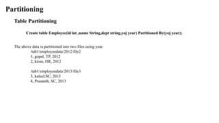
Partitioning
Table Partitioning
Create a table with Partition using the command :
CREATE [EXTERNAL] Table <table name> (<column name 1> <datatype 1> ….)
PARTITIONED BY ((<column name n> <datatype n> [COMMENT <column comment>,…);
Example
The following file contains employeedata table.
/tab1/employeedata/file1
id, name, dept, yoj
1, gopal, TP, 2012
2, kiran, HR, 2012
3, kaleel, SC, 2013
4, Prasanth, SC, 2013
Suppose you need to retrieve the details of all employees who joined in 2012.
A query searches the whole table for the required information.
However, if you partition the employee data with the year and store it in a separate file, it reduces the query
processing time.

Partitioning
Table Partitioning
Create table Employee(id int ,name String,dept string,yoj year) Partitioned By(yoj year);
The above data is partitioned into two files using year.
/tab1/employeedata/2012/file2
1, gopal, TP, 2012
2, kiran, HR, 2012
/tab1/employeedata/2013/file3
3, kaleel,SC, 2013
4, Prasanth, SC, 2013

Partitioning
Adding a Partition
Add partitions to a table by altering the table. Let us assume we have a table called employee with
fields such as Id, Name, Salary, Designation, Dept, and yoj.
ALTER TABLE table_name ADD [IF NOT EXISTS] PARTITION partition_spec
[LOCATION 'location1'] partition_spec [LOCATION 'location2'] ...;
partition_spec:
: (p_column = p_col_value, p_column = p_col_value, ...)
The following query is used to add a partition to the employee table.
hive> ALTER TABLE employee
> ADD PARTITION (year=’2012’)
> location '/2012/part2012';

Partitioning
Renaming a Partition
The syntax of this command is as follows.
ALTER TABLE table_name PARTITION partition_spec RENAME TO PARTITION partition_spec;
The following query is used to rename a partition:
hive> ALTER TABLE employee PARTITION (year=’1203’)
> RENAME TO PARTITION (Yoj=’1203’);

Partitioning
Dropping a Partition
The following syntax is used to drop a partition:
ALTER TABLE table_name DROP [IF EXISTS] PARTITION partition_spec,
PARTITION partition_spec,...;
The following query is used to drop a partition:
hive> ALTER TABLE employee DROP [IF EXISTS]
> PARTITION (year=’1203’);

HiveQL For Querying the Data : Select-Where
The Hive Query Language (HiveQL) is a query language for Hive to process and analyze structured data
in a Metastore.
SELECT statement is used to retrieve the data from a table. WHERE clause works similar to a condition.
It filters the data using the condition and gives you a finite result. The built-in operators and functions
generate an expression, which fulfils the condition.
Given below is the syntax of the SELECT query:
SELECT [ALL | DISTINCT] select_expr, select_expr, ...
FROM table_reference
[WHERE where_condition]
[GROUP BY col_list]
[HAVING having_condition]
[CLUSTER BY col_list | [DISTRIBUTE BY col_list] [SORT
BY col_list]]
[LIMIT number];

Aggregation
Hive supports the following built-in aggregation functions. The usage of these functions
is same as the SQL aggregate functions.

Order By
The ORDER BY clause is used to retrieve the details based on one column
and sort the result set by ascending or descending order.
Example :
Assume employee table as given below, with the fields named Id, Name,
Salary, Designation, and Dept. Generate a query to retrieve the employee
details in order by using Department name.
The following query retrieves the employee details
hive> SELECT Id, Name, Dept FROM employee ORDER BY DEPT;

Group By
The GROUP BY clause is used to group all the records in a result set using a particular collection
column. It is used to query a group of records.
Example :
Generate a query to retrieve the number of employees in each
department.
The following query retrieves the employee details
hive> SELECT Dept,count(*) FROM employee GROUP BY DEPT;

JOIN is a clause that is used for combining specific fields from two tables by using values common to each one.
It is used to combine records from two or more tables in the database.
Joins
Syntax
table_reference JOIN table_factor [join_condition]
| table_reference {LEFT|RIGHT|FULL} [OUTER] JOIN table_reference
join_condition
| table_reference LEFT SEMI JOIN table_reference join_condition
| table_reference CROSS JOIN table_reference [join_condition]

Joins
Consider the following table named CUSTOMERS.. Consider table ORDERS
JOIN clause is used to combine and retrieve the records from multiple tables. JOIN is same as OUTER JOIN in SQL. A
JOIN condition is to be raised using the primary keys and foreign keys of the tables.
hive> SELECT c.ID, c.NAME, c.AGE, o.AMOUNT
FROM CUSTOMERS c JOIN ORDERS o
ON (c.ID = o.CUSTOMER_ID);

Joins
LEFT OUTER JOIN
The HiveQL LEFT OUTER JOIN returns all the rows from the left table, even if there are no matches in the
right table.
This means, if the ON clause matches 0 (zero) records in the right table, the JOIN still returns a row in the
result, but with NULL in each column from the right table.
A LEFT JOIN returns all the values from the left table, plus the matched values from the right table, or NULL
in case of no matching JOIN predicate.

Joins
LEFT OUTER JOIN
hive> SELECT c.ID, c.NAME, o.AMOUNT, o.DATE
FROM CUSTOMERS c
LEFT OUTER JOIN ORDERS o

Joins
RIGHT OUTER JOIN
The HiveQL RIGHT OUTER JOIN returns all the rows from the right table, even if there are no
matches in the left table.
If the ON clause matches 0 (zero) records in the left table, the JOIN still returns a row in the
result, but with NULL in each column from the left table.
A RIGHT JOIN returns all the values from the right table, plus the matched values from the left
table, or NULL in case of no matching join predicate.

Joins
RIGHT OUTER JOIN
hive> SELECT c.ID, c.NAME, o.AMOUNT,
o.DATE FROM CUSTOMERS c RIGHT OUTER
JOIN ORDERS o ON (c.ID = o.CUSTOMER_ID);

Joins
FULL OUTER JOIN
The HiveQL FULL OUTER JOIN combines the records of both the left and the right
outer tables that fulfil the JOIN condition.
The joined table contains either all the records from both the tables, or fills in NULL
values for missing matches on either side.

Joins
FULL OUTER JOIN
hive> SELECT c.ID, c.NAME, o.AMOUNT, o.DATE
FROM CUSTOMERS c
FULL OUTER JOIN ORDERS o

View
Views are generated based on user requirements.
You can save any result set data as a view.
The usage of view in Hive is same as that of the view in SQL. It is a standard RDBMS concept.
We can execute all DML operations on a view.
Creating a View
create a view at the time of executing a SELECT statement.
The syntax is as follows:
CREATE VIEW [IF NOT EXISTS] view_name
[(column_name [COMMENT column_comment], ...) ]
[COMMENT table_comment]
AS SELECT ...
Dropping a View
DROP VIEW view_name

View
Example
Assume employee table as given below, with the fields Id,
Name, Salary, Designation, and Dept.
Generate a query to retrieve the employee details who earn a
salary of more than Rs 30000. We store the result in a view
named emp_30000.
hive> CREATE VIEW emp_30000 AS
SELECT * FROM employee
WHERE salary>30000;

PIG
 Is an abstraction over MapReduce
 Is an execution framework for parallel processing
 Reduces the complexities of writing a MapReduce program
 Is a high-level dataflow language. Dataflow language means that a Pig operation node
takes the inputs and generates the output for the next node
 Is mostly used in HDFS environment
 Performs data manipulation operations at files at data nodes in Hadoop.

Applications of Apache Pig
Applications of Pig are:
 Analyzing large datasets
 Executing tasks involving adhoc processing
 Processing large data sources such as web logs and streaming online data
 Data processing for search platforms. Pig processes different types of data
 Processing time sensitive data loads; data extracts and analyzes quickly. For example,
analysis of data from twitter to find patterns for user behavior and recommendations.

Features
(i) Apache PIG helps programmers write complex data transformations using scripts (without using Java).
Pig Latin language is very similar to SQL and possess a rich set of built-in operators, such as group, join,
filter, limit, order by, parallel, sort and split. It provides an interactive shell known as Grunt to write Pig
Latin scripts.
(ii) Creates user defined functions (UDFs) to write custom functions which are not available in Pig. A UDF
can be in other programming languages, such as Java, Python, Ruby, Jython, JRuby. They easily embed
into Pig scripts written in Pig Latin. UDFs provide extensibility to the Pig.
(iii) Process any kind of data, structured, semi-structured or unstructured data, coming from various sources.
(iv) Reduces the length of codes using multi-query approach. Pig code of 10 lines is equal to MapReduce
code of 200 lines. Thus, the processing is very fast.

(v) Extracts the data, performs operations on that data and dumps the data in the required format in
HDFS. The operation is called ETL (Extract Transform Load).
(vi) Performs automatic optimization of tasks before execution.
(vii) Programmers and developers can concentrate on the whole operation without a need to create
mapper and reducer tasks separately.
(viii) Reads the input data files from HDFS or the data files from other sources such as local file
system, stores the intermediate data and writes back the output in HDFS.
(ix) Pig characteristics are data reading, processing, programming the UDFs in multiple
languages and programming multiple queries by fewer codes. This causes fast processing.
(x) Pig derives guidance from four philosophies, live anywhere, take anything, domestic and run as
if flying. This justifies the name Pig, as the animal pig also has these characteristics.

Differences between Pig and MapReduce

Differences between Pig and SQL

Differences between Pig and Hive

The three ways to execute scripts are:
1. Grunt Shell: An interactive shell of Pig that executes the scripts.
2. Script File: Pig commands written in a script file that execute at Pig Server.
3. Embedded Script: Create UDFs for the functions unavailable as Pig built-in
operators. UDF can be in other programming languages. The UDFs can embed in
Pig Latin Script file.

1. Parser
A parser handles Pig scripts after passing through Grunt or Pig Server.
The Parser performs type checking and checks the script syntax.
The output is a Directed Acyclic Graph (DAG).
DAG represents the Pig Latin statements and logical operators. Nodes represent the
logical operators. Edges between sequentially traversed nodes represent the
dataflows.

2. Optimizer
The DAG is submitted to the logical optimizer.
The optimization activities, such as split, merge, transform and reorder operators execute in
this phase.
The optimization is an automatic feature.
The optimizer reduces the amount of data in the pipeline at any instant of time, while
processing the extracted data.
It executes certain functions for carrying out this task, as explained as follows:

PushUpFilter: If there are multiple conditions in the filter and the filter can be split, Pig splits the
conditions and pushes up each condition separately. Selecting these conditions at an early stage helps in
reducing the number of records remaining in the pipeline.
PushDownForEachFlatten: Applying flatten, which produces a cross product between a complex type
such as a tuple, bag or other fields in the record, as late as possible in the plan. This keeps the number of
records low in the pipeline.
ColumnPruner: Omitts never used columns or the ones no longer needed, reducing the size of the record.
This can be applied after each operator, so that the fields can be pruned as aggressively as possible.
MapKeyPruner: Omitts never used map keys, reducing the size of the record.
2. Optimizer

LimitOptimizer: If the limit operator is immediately applied after load or sort operator, Pig
converts the load or sort into a limit-sensitive implementation, which does not require
processing the whole dataset. Applying the limit earlier reduces the number of records.
3. Compiler The compiler compiles after the optimization process. The optimized codes
are a series of MapReduce jobs.
4. Execution Engine Finally, the MapReduce jobs submit for execution to the engine.
The MapReduce jobs execute and it outputs the final result.

Apache Pig -Grunt Shell
Main use of Grunt shell is for writing Pig Latin scripts.
Any shell command invokes using sh and ls.
Syntax of sh command is:
grunt> sh shell command parameters
Syntax of ls command:
grunt> sh ls

Pig Latin Data Model
Pig Latin supports primitive data types which are atomic or scalar data types. Atomic data types are
int, float, long, double, char[], byte [].
The language also defines complex data types. Complex data types are tuple, bag and map.

Pig Latin enables developing the scripts for data analysis.
A number of operators in Pig Latin help to develop their own functions for reading, writing and processing data.
Pig Latin programs execute in the Pig run-time environment.
Pig Latin and Developing Pig Latin scripts
Pig Latin : Order of Processing Pig Statements
 Basic constructs to process the data.
 Include schemas and expressions.
 End with a semicolon.
 LOAD statement reads the data from file system, DUMP displays the result and STORE stores the result.
 Single line comments begin with - - and multiline begin with/* and end with*/
 Keywords (for example, LOAD, STORE, DUMP) are not case-sensitive. Function names, relations and paths are
case-sensitive.
 Function names ,relations and paths are case sensitive.

Pig Latin and Developing Pig Latin scripts
Order of Processing Pig Statements

Apache Pig Execution
Pig Execution Modes
Local Mode: All the data files install and run from a local host using the local file system. Local
mode is mostly used for testing purpose.
COMMAND:
pig -x local
MapReduce Mode:
All the data files load or process that exists in the HDFS. A MapReduce job invokes in the back-end
to perform a particular operation on the data that exists in the HDFS when a Pig Latin statement
executes to process the data.
COMMAND:
pig -x mapreduce or pig

Pig Latin Script Execution Modes
 Interactive Mode - Using the Grunt shell.
 Batch Mode - Writing the Pig Latin script in a single file with .pig extension.
 Embedded Mode - Defining UDFs in programming languages such as
Java, and using them in the script.

Commands
 To get the list of pig commands: pig-help;
 To get the version of pig: pig -version.
 To start the Grunt shell, write the command: pig
LOAD Command The first step to a dataflow is to specify the input.
Load statement in Pig Latin loads the data from PigStorage.
To load data from HBase: book load 'MyBook' using HBaseStorage();
For reading CSV file, PigStorage takes an argument which indicates which character to use
as a separator.
For example,
book = LOAD 'PigDemo/Data/Input/myBook.csv' USING PigStorage (,);
To specify the data-schema for loading: book = LOAD 'MyBook' AS (name, author, edition,
publisher);

Commands
Store Command Pig provides the store statement for writing the processed data after
the processing is complete. It is the mirror image of the load statement in certain
ways.
By default, Pig stores data on HDFS in a tab-delimited file using PigStorage:
STORE processed into '/PigDemo/Data/Output/Processed';
To store in HBaseStorage with a using clause:
STORE processed into 'processed' using HBaseStorage();
To store data as comma-separated text data, PigStorage takes an argument to
indicate which character to use as a separator:
STORE processed into 'processed' using PigStorage(',');

Commands
Dump Command Pig provides dump command to see the processed data on the screen.
This is particularly useful during debugging and prototyping sessions. It can also be
useful for quick adhoc jobs.
The following command directs the output of the Pig script on the display screen:
DUMP processed;

Big Data Tools MapReduce,Hive and Pig.pdf

Recommended

More Related Content

Similar to Big Data Tools MapReduce,Hive and Pig.pdf (20)

More from SharmilaChidaravalli (11)

Recently uploaded (20)

Big Data Tools MapReduce,Hive and Pig.pdf