SlideShare a Scribd company logo
CAPITAL BUDGETING
DECISION-MAKING IN
TELECOM SECTOR USING
REAL OPTION ANALYSIS
Master’s Thesis presentation
Mentor: Prof. Aleš Berk
Candidate: Dimitar Serafimov
Ljubljana, May, 2013
Introduction
Implementing risks techniques in capital budgeting decisions is
becoming increasingly more important, as:
• Recourses are getting scarcer;
• Competition is becoming more intense;
• The expenditures are large;
• The uncertainty related to the advanced technology is higher
• Regulators are increasing the requirements / constrains for
the operators with significant market power
• Business models are changing, etc.
The need for additional information related to uncertainty is of a
major importance for decision makers, as decisions made today
will definitely impact the future
Problem Description
The workhorse in capital decision making – Discounted Cash
Flow analysis or NPV
Primarily used and invented for evaluating financial assets,
which are passive by their nature
In contrast, Real assets are dynamic - management has options
to influence the project and thus alter the outcome of the
investment.
The mechanic of DCF analysis involves
forecasting the expected incremental net
cash flows of the project and discounting
them back to today with discount factor,
usually the WACC.
Problem Description cont‟d.
There are several problem in this technique:
• Beta is an estimate from past market
performance, while its application throughout
WACC is intended for the future project
performance
• The correlation between the asset and the market
is diluting the discount factor especially with low
correlated, but highly volatile asset because beta
is measure of both the correlation and the volatility
• The third is application of constant discount rate to
non constant future cash flows or non constant
uncertainty
• Can not accommodate the managements„
flexibility
Problem Description cont‟d.
Management has the opportunity alter the passive operating
strategy, hence modify the project‟s outcome
This opportunity to take action is in fact an option – a right, but
not an obligation.
As the underlying asset is real, Stewart Myers has coined the
term Real Options as to distinguish them from Financial Options
The Thesis
Managements‟ flexibility brings additional value over and above
the passive operating strategy – options are valuable
expanded NPV= passive NPV + value of the option
Not considering the embedded options leads to
underinvestment strategies
Thus the model for valuing future opportunities has to be
amended in order to reflect its true potential.
The Research
1.Qualitative review of the related literature
• Theoretical background
• Specific application of ROA, with focus on the
Telecommunication sector
2. Quantitative application of the models and techniques on a
particular project - FTTH
• Several types of Options
• Option to differ the investment
• Option to contract the investment
• Growth option
The Research cont‟d.
• Different calculation methodologies
• Closed form solution
• Lattices
• Simulation
• Application of five different parameterizations for
approximation of the diffusion process
Qualitative - application of ROA
Most extensive application of ROA in
• Natural resources utilization – Oil and Mining sector
• Pharmaceutical, specifically R & D
Due to:
• Capital intensity
• Availability of traded assets – option
• High uncertainty
Application of ROA in Telecommunication sector:
• With the beginning of deregulation of the sector and
regulation Telecom operators with significant market power
• Mostly for justification of costs and allowable investment base
• Only recently for application of new technologies
Qualitative - Required assumptions -
cont‟d
Conditions for application of Financial assets valuation tools to
valuation of Real assets
ROA is considered as an extension to the DCF/NPV analysis,
not as a substitute hence:
• average rational investor is a risk averse
• prefers more to less wealth
All option pricing models are based on the concept of riskless
hedge and no arbitrage opportunities hence:
• The market is complete - any state of the world can be
replicated by some combination of the existing securities.
Qualitative - Required assumptions -
cont‟d
• Complete market for Binomial - there are at least two linearly
independent securities:
• a twin security and a
• riskless bond
• Black - Scholes assumptions:
• There are no transaction costs;
• The investor may borrow any fraction of the purchase price at the short
term risk free interest rate;
• Short selling is permitted;
• The call option can be exercised only on its expiration date;
• Trading of securities takes place continuously;
• The stock price (underlying asset) follows a geometric Brownian motion
with constant drift and volatility, and
• The underlying security does not pay dividends.
Qualitative - Required assumptions -
cont‟d
The diffusion process – changes of the underlying asset value
• Geometric Brownian motion - continuous stochastic process,
with small random movements
• Pure jump process, each successive asset price is almost
the same as the previous price, but only occasionally with
low probability of occurrence significantly different
• Combination
• It has to correspond to the actual asset being analyzed
Qualitative - Required assumptions -
cont‟d
Incomplete market - partially solved by so called the integrated
– two risks type approach
The additional assumptions / conditions for this so called
“Partially complete market” are:
• Securities depend only on market states,
• The market is complete with respect to the market
uncertainties and
• Private events convey no information about future market
events.
Disaggregation of uncertainties
Drawback: Private and Market uncertainties might be correlated
Qualitative – Option valuation
techniques
Categorized in three broader valuation techniques:
1. Partial differential equations
- Black – Scholes as a closed – form solution
- Analytical approximations
- Numerical methods, such as finite difference method
2. Simulations
- Monte Carlo
3. Lattices
- Binomial
- Trinomial
- Quadrinomial
- Multinomial
Options
Strike or
Exercise price
Price of underlying asset
Net Payoff
Out-of-the-money In-the-money
At-the-money
Strike or
Exercise price
Price of underlying asset
Net Payoff
In-the-money Out-of-the-money
At-the-money
Payoff of Call Option Payoff of Put Option
Qualitative - Option valuation
techniques
Black – Scholes as a closed – form
solution
Where C is the value of the call option
S0 is the current value of the underlying
asset;
X is the cost of investing or strike price;
r risk free rate of return;
T is the time to expiration or validity of
the real option;
N(d1) and N(d2) are values from normal
standard distribution
is the volatility
r is the risk-free rate
𝐶 = 𝑁 𝑑1 𝑆0 − 𝑁 𝑑2 𝑋𝑒−𝑟𝑇 𝑑1 =
𝑙𝑛
𝑆𝑜
𝑋
+ 𝑟 +
𝜎2
2
𝑇
𝜎 𝑇
𝑑2 = 𝑑1 − 𝜎 𝑇
0
0.2
0.4
0.6
0.8
1
1.2
-3.00
-2.50
-2.00
-1.50
-1.00
-0.50
0.00
0.50
1.00
1.50
2.00
2.50
3.00
Qualitative - Option valuation
techniques
Simulations
is the volatility
St and St-1 are the values of the underlying asset at
time t and t-1
t is the time increment
r is the risk free rate of return
is value from normal standard distribution with mean
zero and a variance of 1.0.
𝑆𝑡 = 𝑆𝑡−1 + 𝑆𝑡−1(𝑟 𝛿𝑡 + 𝜎𝜀 𝛿𝑡) 𝑚𝑎𝑥 𝑆𝑡 − 𝑋, 0
-1.50
-1.00
-0.50
0.00
0.50
1.00
1.50
0 0.2 0.4 0.6 0.8 1 1.2Time
Wiener Process Z w/o Drift
+STDEV(Z)=
+SQRT(T)
-STDEV(Z)=-
SQRT(T)
Qualitative - Option valuation
techniques
Lattices – Binomial
𝑢 = 𝑒(𝜎 𝛿𝑡)
𝑑 = 𝑒−(𝜎 𝛿𝑡)
𝑝 =
𝑒(𝑟𝛿𝑡 )
− 𝑑
𝑢 − 𝑑
𝛿𝑡 =
𝑇
𝑛
𝐶 =
𝑛!
𝑗! 𝑛 − 𝑗 !
𝑛
𝑗=0 𝑝 𝑗
1 − 𝑝 𝑛−𝑗
𝑚𝑎𝑥 0, 𝑢 𝑗
𝑑 𝑛−𝑗
𝑆0 − 𝑋
𝑒 𝑟𝛿𝑡
𝑝 =
𝑒(𝑟−𝑦)𝛿𝑡 −𝑑
𝑢−𝑑
S0
S0u
S0d
S0u2
S0ud
S0d2
S0u3 1/8
S0u2d 3/8
S0du2 3/8
S0d3 1/8
0 1 2 3
Time increments
Qualitative Option valuation techniques
Lattices – Qudrinomial
S0
S0u1u2
S0u1d2
S0u12u2d2
S0u12u22
S0u1u2d1d2
S0u1d1u22
S0u12d22
S0u12u2d2
S0u1d1d22
S0u1u2d1d2
S0d1u2
S0d1d2
S0u1u2d1d2
S0u1d1u22
S0d12u2d2
S0d12u22
S0u1d1d22
S0u1d1u2d2
S0d12d22
S0 d12u2d2
Qualitative research – Integration of
DTA
S0
S0
u
S0
udx1
S0
u
2
x1
S0
udy1
S0
u
2
y1
S0
d
S0
d
2
x1
S0
udx1
S0
d
2
y1
S0
udy1
p p1
(1-p) p1
p(1-p1
)
(1-p)(1-p1
)
p p1
(1-p) p1
p(1-p1
)
(1-p)(1-p1
)
Where
x1 and y1 are asset
correction factors
Quantitative FTTH
Fiber optical network
Quantitative - FTTH DCF
FTTH DCF Analysis
Year 0 1 2 3 4 5 6
FTTH Residential & Business Fast Internet customers - new sales100% 8700 20000 28000 44000 10000 6000
WS participation in total sales 10% 20% 20% 20% 20%
Distribution of FTTH Fast Internet customers
Residential 59% 50% 50% 50% 50% 50%
Residential +HD TV 32% 41% 41% 41% 41% 41%
Business 10% 10% 10% 10% 10% 10%
FTTH incremental monthly fee
Residential monthly fee - FTTH Fast Internet € 4,5 € 4,2 € 3,9 € 3,9 € 3,9 € 3,9
Residential monthly fee - FTTH Fast Internet and HD TV € 10,0 € 9,3 € 8,6 € 8,6 € 8,6 € 8,6
Business monthly fee - FTTH Fast Internet € 11,0 € 10,2 € 9,5 € 9,5 € 9,5 € 9,5
Average Rate Per User (ARPU) € 24,0 € 24,0 € 23,0 € 22,0 € 22,0 € 22,0
Revenues
Residential monthly fee - FTTH Fast Internet € 137.417 € 464.861 € 781.585 € 1.149.390 € 1.126.402 € 367.805
Residential monthly fee - FTTH Fast Internet and HD TV € 164.430 € 845.203 € 1.421.064 € 2.089.800 € 2.048.004 € 668.736
Business monthly fee - FTTH Fast Internet € 57.420 € 229.561 € 385.968 € 567.600 € 556.248 € 181.632
ARPU revenues € 1.252.800 € 5.385.600 € 11.785.200 € 20.776.800 € 27.904.800 € 30.808.800
Total Revenues € 1.612.067 € 6.925.225 € 14.373.817 € 24.583.590 € 31.635.454 € 32.026.973
Cost margin as % of sales 50% 40% 39% 38% 37% 36%
Total operating costs € 806.033 € 2.770.090 € 5.605.789 € 9.341.764 € 11.705.118 € 11.529.710
EBITDA € 806.033 € 4.155.135 € 8.768.028 € 15.241.826 € 19.930.336 € 20.497.263
Depreciation € 1.089.866 € 2.858.296 € 4.950.663 € 6.670.126 € 6.399.402 € 5.556.420
EBIT -€ 283.833 € 1.296.839 € 3.817.366 € 8.571.700 € 13.530.934 € 14.940.842
Tax @ 10% 10% € 0 € 129.684 € 381.737 € 857.170 € 1.353.093 € 1.494.084
Net income -€ 283.833 € 1.167.155 € 3.435.629 € 7.714.530 € 12.177.841 € 13.446.758
Operating cash flow (CF) € 806.033 € 4.025.451 € 8.386.292 € 14.384.656 € 18.577.243 € 19.003.178
Present value (PV) CF @ 13.6% WACC € 709.536 € 3.119.305 € 5.720.513 € 8.637.462 € 9.819.505 € 8.842.117
CF PV cumulative € 709.536 € 3.828.842 € 9.549.355 € 18.186.817 € 28.006.322 € 36.848.439
Capital expenditures (CAPEX) € 7.933.494 € 10.055.587 € 12.351.415 € 8.046.443 € 3.283.084 € 2.236.696 € 0
CAPEX PV @ 13.6% WACC € 7.933.494 € 8.851.749 € 9.571.060 € 5.488.693 € 1.971.373 € 1.182.267 € 0
Total CAPEX PV € 34.998.635
CF PV cummulative - CAPEX PV cummulative -€ 34.998.635 -€ 34.289.099 -€ 31.169.793 -€ 25.449.280 -€ 16.811.818 -€ 6.992.313 € 1.849.804
Net Present Value (NPV) as of Y6 € 1.849.804
Discounted payback period (Years) 5,79
Internal rate of return (IRR) 15,79%
Quantitative FTTH input estimates
Method annual volatility in %
Implied volatility B-S model 27.47
Logarithmic CF from project returns 29.70
Logarithmic stock price returns 30.91
Standard deviation in firm value1
40.64
Inputs Date
Stock price € 8,68 05.03.2012
Dividend € 0,70
Dividend yield 8,06%
Call option value 0,9 05.03.2012
Exercise price 8 21.06.2013
Risk - free rate (annual) dis. 0,13%
Risk - free rate (annual) con. 0,13%
Black Scholes calculator
INPUTS OUTPUTS
Standard deviation (annual) 27,47% d1 0,088264
Maturity (in years) 1,30 d2 -0,22446
Risk - free rate (annual) 0,13% N(d1) 0,535167
Stock price € 8,68 N(d2) 0,4112
Exercise price € 8,00 B-S call 0,900052
Divident yield (annual) 8% B-S put 1,068341
12 23.01.2012-27.01.2012 511 -0,004 8,50322E-07
13 16.01.2012-20.01.2012 513 -0,004 8,78585E-07
14 09.01.2012-13.01.2012 515 -0,002 8,34354E-06
15 03.01.2012-05.01.2012 516 -0,008 8,37328E-06
16 26.12.2011-29.12.2011 520 0,000 2,33133E-05
17 19.12.2011-23.12.2011 520 -0,010 2,24777E-05
18 12.12.2011-16.12.2011 525 0,006 0,000111494
19 05.12.2011-09.12.2011 522 -0,015 0,000107766
20 28.11.2011-02.12.2011 530 0,019 0,000570091
21 21.11.2011-25.11.2011 520 0,016 0,000413413
22 14.11.2011-18.11.2011 512 0,010 0,000214388
23 07.11.2011-11.11.2011 507 0,002 4,6277E-05
24 31.10.2011-04.11.2011 506 0,002 4,63301E-05
25 24.10.2011-28.10.2011 505 0,000 2,33133E-05
26 17.10.2011-21.10.2011 505 0,000 2,33133E-05
27 10.10.2011-14.10.2011 505 0,000 2,33133E-05
28 03.10.2011-07.10.2011 505 -0,002 8,12332E-06
29 26.09.2011-30.09.2011 506 -0,004 7,80759E-07
30 19.09.2011-23.09.2011 508 0,006 0,000115593
31 12.09.2011-16.09.2011 505 -0,010 2,52397E-05
32 05.09.2011-09.09.2011 510 -0,004 8,36282E-07
33 29.08.2011-02.09.2011 512 0,004 7,64275E-05
34 22.08.2011-26.08.2011 510 0,016 0,000425968
35 15.08.2011-19.08.2011 502 -0,006 1,27673E-06
36 08.08.2011-12.08.2011 505 0,006 0,000116353
37 01.08.2011-05.08.2011 502 0,002 4,65452E-05
38 25.07.2011-29.07.2011 501 0,000 2,33133E-05
39 18.07.2011-22.07.2011 501 0,000 2,33133E-05
40 11.07.2011-15.07.2011 501 -0,004 7,12868E-07
41 04.07.2011-08.07.2011 503 0,006 0,000116866
42 27.06.2011-01.07.2011 500 0,000 2,33133E-05
43 20.06.2011-24.06.2011 500 -0,002 8,01106E-06
44 13.06.2011-17.06.2011 501 -0,002 8,03363E-06
45 06.06.2011-09.06.2011 502 -0,006 1,27673E-06
46 30.05.2011-03.06.2011 505 0,012 0,000281592
47 23.05.2011-27.05.2011 499 0,018 0,000530339
48 16.05.2011-20.05.2011 490 -0,002 7,78213E-06
49 09.05.2011-13.05.2011 491 -0,008 1,07929E-05
50 03.05.2011-06.05.2011 495 0,031 0,001267363
51 26.04.2011-29.04.2011 480 0,043 0,002245622
52 18.04.2011-21.04.2011 460 -0,264 0,067188126
53 11.04.2011-15.04.2011 599 / /
Average -0,005
Total 0,101483
4,46%
30,91%
Weekly volatility
Yearly volatility
Quantitative – Option to defer
Step 0 1
Factors
u= 1,362
d= 0,734
p= 0,524
44,19
Sou e
32,44 8,69
So k
4,28 23,81
Sod k
0,00
Related decision
e - exercise the option
k- keep the option
𝑉 =
𝑝 𝑚𝑎𝑥 0, 𝑢 𝑆0 − 𝑋 + 1 − 𝑝 𝑚𝑎𝑥 0, 𝑑 𝑆0 − 𝑋
𝑒 𝑟𝛿𝑡
The input parameters (in million €) are as follows:
Stock price (PV of the cash flow as of now) S0= 32.4
Exercise price (PV of the investment as of Year 1) X=35.5
Standard deviation (annual volatility of the asset) =30.9%
Risk-free rate (continuous) rf=6.1%
Time to expiration T=1 Year
Time step t=1
BS yields 3.58 million €
Simulation yields 3.98 million €
Quantitative – Option to defer
Step 0 1 2 3 4 5
Factors 64,75
u= 1,148 Sou5
e
d= 0,871 56,39 29,25
p= 0,510 Sou4
k
49,11 21,32 49,11
Sou3
k Sou4
d e
14,47 42,77 13,61
42,77 Sou3
d k
Sou2
k 37 7,70 37,25
37,25 9,37 Sou2
d k Sou3
d2
e
Sou k 4,30 1,75
32,44 5,87 32,44 32,44
So k Soud k Sou2
d2
k
3,59 28,25 2,38 0,88
Sod k 28,25 28,25
1,31 24,60 Soud2
k Sou2
d3
k
Sod2
k 0,44 24,60 0,00
0 Soud3
k
Related decision 21 0,00 21,43
e - exercise the option Sod3
k Soud4
k
k- keep the option 0 19 0,00
Sod4
k
0,00 16,25
Sod5
k
0,00
Quantitative
Method
Annual volatility
in
Binomial
1 step
Binomial
5 steps
B-S
model
Standard deviation in firm value 40,64 5,90 4,95 4,84
Logarithmic stock price returns 30,91 4,28 3,59 3,58
Logarithmic CF from project returns 29,70 4,07 3,59 3,58
Implied volatility B-S model 27,47 3,69 3,42 3,43
Option value in 1.000.000 EUR
The option value is highly sensitive to the time step and
the volatility
Quantitative Different parameterizations
Trigeorgis
𝜇 =
𝛼
𝜎2
−
1
2
(23)
𝑘 = 𝜎 𝛿𝑡 (24)
ℎ = 𝑘2 + (𝑘2 𝜇)2 (25)
𝑝 =
1
2
(1 +
𝑘2 𝜇
ℎ
) (26)
𝜇 =
𝛼
𝜎2
−
1
2
(23)
𝑘 = 𝜎 𝛿𝑡 (24)
ℎ = 𝑘2 + (𝑘2 𝜇)2 (25)
𝑝 =
1
2
(1 +
𝑘2 𝜇
ℎ
) (26)
𝑢 = 𝑒
𝑟−
𝜎2
2
𝛿𝑡+𝜎 𝛿𝑡
(27)
𝑑 = 𝑒
𝑟−
𝜎2
2
𝛿𝑡−𝜎 𝛿𝑡
(28)
𝑢𝑑 = 𝑒
2 𝑟−
𝜎2
2
𝛿𝑡
(29)
𝑢 = 𝑒
𝑟−
𝜎2
2
𝛿𝑡+𝜎 𝛿𝑡
(27)
𝑑 = 𝑒
𝑟−
𝜎2
2
𝛿𝑡−𝜎 𝛿𝑡
(28)
𝑢𝑑 = 𝑒
2 𝑟−
𝜎2
2
𝛿𝑡
(29)
= r-
𝑢 = 𝑒ℎ
,
𝑑 = 𝑒−ℎ
𝑒 𝜎2 𝛿𝑡 − 1𝑢 = 𝑒 𝑒 𝜎2 𝛿𝑡 −1+𝑟𝛿𝑡
𝑑 = 𝑒− 𝑒 𝜎2 𝛿𝑡 −1+𝑟𝛿𝑡
𝑝 =
𝑒 𝑟𝛿𝑡
− 𝑑
𝑢 − 𝑑
Rendelmann – Bartter
Hull
𝑝 =
1
2
𝜎 𝛿𝑡
Haahtela
Quantitative Different parameterizations
0,00
0,50
1,00
1,50
2,00
2,50
3,00
3,50
4,00
4,50
5,00
1 2 5 10
Project value
[millionEUR]
number of steps n
BS
CRR
RB
Trigerogis
Hull
Haahtela
=30,9%
Option to defer the investment for one year
Quantitative Different parameterizations
-1
0
1
2
3
4
5
6
0% 5% 10% 15% 20% 25% 30% 35% 40% 45%
Project value
[million €]
Volatility
BS
CRR
Trigeorgis
RB
Hull
Haahtela
0
0.5
1
1.5
2
5% 10% 15% 20%
Option to Differ the Investment (Double Step) With Different
Parameterizations in Relation to Volatility
Quantitative Different parameterizations
Method
Annual
volatility
in %
BS model in
1.000.000
EUR
CRR 1
step
RB 1
step
Trigerogis 1
step
Hull 1
step
Haahtela
1 step
Standard deviation in firm value 40,64 4,8347 22,07 18,38 21,92 27,93 32,23
Logarithmic stock price returns 30,91 3,5818 19,47 21,86 19,17 23,05 30,92
Logarithmic CF from project returns 29,70 3,4251 18,90 22,27 18,71 22,24 30,83
Implied volatility B-S model 27,47 3,1371 17,55 22,98 17,68 20,46 30,66
Assumed volatility 20,00 2,1707 8,32 25,29 11,57 10,04 30,59
Assumed volatility 10,00 0,8889 -70,76 27,97 -30,71 -70,04 31,59
Assumed volatility 7,00 0,5184 -100,00 26,27 -94,02 -100,00 30,04
17,26 22,16 17,81 20,74 31,04
5,26 2,50 3,83 6,59 0,68Standard deviation of higher (20% and above) volatilities
Average of higher (20% and above) volatilities
Relative error between different parameterizations and
B-S as reference in %
Method
Annual
volatility
in %
BS model in
1.000.000 EUR
CRR 2
steps RB 2 steps
Trigerogis
2 steps
Hull 2
steps
Haahtela 2
steps
Standard deviation in firm value 40,64 4,8347 0,00 1,70 -0,13 -2,05 5,89
Logarithmic stock price returns 30,91 3,5818 2,94 1,09 2,72 -4,19 5,54
Logarithmic CF from project returns 29,70 3,4251 3,40 1,04 3,21 -4,56 5,42
Implied volatility B-S model 27,47 3,1371 4,29 0,97 4,22 -5,31 5,16
Assumed volatility 20,00 2,1707 7,69 1,28 8,71 -8,29 3,50
Assumed volatility 10,00 0,8889 -2,82 6,41 12,45 2,56 -4,06
Assumed volatility 7,00 0,5184 -63,46 12,37 -7,57 63,23 -10,99
3,67 1,21 3,75 -4,88 5,10
2,77 0,29 3,21 2,26 0,93
Average of higher (20% and above) volatilities
Standard deviation of higher (20% and above) volatilities
Relative error between different parameterizations and B-S
as reference in %
Single step
Double step
Quantitative Different parameterizations
Five step
Ten step
Method Annual volatility
in %
BS model in
1.000.000 EUR CRR 5 step RB 5 step
Trigerogis 5
step
Hull 5
step
Haahtela
5 step
Standard deviation in firm value 40,64 4,8347 2,40 0,56 2,35 3,36 6,09
Logarithmic stock price returns 30,91 3,5818 0,25 1,71 0,16 0,83 5,72
Logarithmic CF from project returns 29,70 3,4251 -0,20 1,82 -0,27 0,35 5,67
Implied volatility B-S model 27,47 3,1371 -1,19 1,99 -1,21 -0,71 5,58
Assumed volatility 20,00 2,1707 -7,28 2,23 -6,98 -7,09 5,09
Assumed volatility 10,00 0,8889 0,18 -1,18 4,89 0,26 1,39
Assumed volatility 7,00 0,5184 -23,24 -8,43 -5,48 -23,17 -6,02
-1,20 1,66 -1,19 -0,65 5,63
Standard deviation of higher (20% and above) volatilities 3,64 0,65 3,49 3,90 0,36
Relative error between different parameterizations and B-
S as reference in %
Average of higher (20% and above) volatilities
Method Annual volatility
in %
BS model in
1.000.000 EUR CRR 10 step RB 10 step
Trigerogis
10 step
Hull 10
step
Haahtela
10 step
Standard deviation in firm value 40,64 4,8347 2,02 2,23 1,99 2,47 -0,16
Logarithmic stock price returns 30,91 3,5818 2,46 2,29 2,42 2,74 0,23
Logarithmic CF from project returns 29,70 3,4251 2,48 2,30 2,45 2,74 0,31
Implied volatility B-S model 27,47 3,1371 2,47 2,32 2,45 2,69 0,47
Assumed volatility 20,00 2,1707 1,20 2,52 1,42 1,33 1,27
Assumed volatility 10,00 0,8889 -0,19 3,38 1,97 -0,16 3,43
Assumed volatility 7,00 0,5184 -11,94 2,53 -6,25 -11,93 3,28
2,13 2,33 2,15 2,39 0,42
Standard deviation of higher (20% and above) volatilities 0,56 0,11 0,45 0,61 0,52
Average of higher (20% and above) volatilities
Relative error between different parameterizations and BS as
reference in %
Quantitative – Inclusion of Dividend
yield
Marke share loss first year in %
Dividend yield
y in %
Binomial
1 step
Binomial
5 steps BS model
Binomial 1
step
Binomial
5 steps
B-S
model
0 0,00 4,28 3,59 3,58 0,524 0,510 0,524
30 0,58 4,20 3,50 3,49 0,514 0,506 0,517
50 0,96 4,15 3,43 3,42 0,507 0,503 0,512
100 1,93 4,02 3,28 3,27 0,491 0,496 0,499
Option value in 1.000.000 EUR p
Quantitative – Integration of DTA into
ROA
S0
S0
u
S0
udx1
S0
u
2
x1
S0
udy1
S0
u
2
y1
S0
d
S0
d
2
x1
S0
udx1
S0
d
2
y1
S0
udy1
p p1
(1-p) p1
p(1-p1
)
(1-p)(1-p1
)
p p1
(1-p) p1
p(1-p1
)
(1-p)(1-p1
)
Step 0 1 2
Factors
u= 1,362 61,25
d= 0,734 Sou2
x1 e
p= 0,524 25,75
p1= 0,100
x1= 1,02 33,01
y1= 1,00 Soudx1 k
44,19 0,00
Sou k
12,22 60,19
Sou2
y1 e
24,69
32,44
Soudy1 k
0,00
32,44
So k
6,02
33,01
Soudx1 k
0,00
17,79
Sod2
x1 k
23,81 0,00
Sod k
0,00 32,44
Soudy1 k
0,00
Related decision 17,48
e - exercise the option Sod2
y1 k
k- keep the option 0,00
Quantitative – Option to contract
The input parameters (in million €) are as follows:
Stock price (PV of the cash flow as of now) S0= 36.85
Savings from contraction cs=16.24
Contraction factor cf = 50%
Standard deviation (annual volatility of the asset) =30.9%
Risk-free rate (continuous) rf=6.1%
Time to expiration T=3 Year
Time step t=1
Step 0 1 2 3
Factors
u= 1,362
d= 0,734
p= 0,524
93,14
Sou3
k
93,14
68,38
Sou2
k 50
50,19 68,38 Sou2
d k
Sou e 50,19
36,85 50,74 36,85
So e Soud e
38,65 27,05 38,06
Sod e 27,05
30,48 19,86 Soud2
e
Sod2
e 29,76
26,17
Related decision 15
e - exercise the option Sod3
e
k- keep the option 23,53
Binomial
Vo=1,8 million €
B-S
Vo=1,45 million €
Quantitative – Sequential compound
Inter-project compoudness
Option on option
Stock price (PV of the cash flow as of now) S0= 36.85
Exercise prices X5= 2.24
X4= 3.28
X3= 8.05
X2= 12.35
X1= 10.06
X0= 7.93
Standard deviation (annual volatility of the asset) =30.9%
Risk-free rate (continuous) rf=6.1%
Time to expiration T=6 Year
Time step t=1
Quantitative – Sequential compound
Step 0 1 2 3 4 5 6
235,43
Factors 172,83 Sou6
e
u= 1,362 Sou5
e 233,19
d= 0,734 126,88 170,59
p= 0,524 Sou4
e 126,88
X5= 2,237 93,14 124,83 93,14 Sou5
d e
Sou3
e Sou4
d e 124,64
91,25 68,38 91,04
68,38 Sou3
d e 68,38
Sou2
e 50 66,40 50,19 Sou4
d2
e
50,19 68,38 Sou2
d e Sou3
d2
e 66,14
Sou e 48,33 48,09
36,85 50,19 36,85 36,85 36,85
So e Soud e Sou2
d2
e Sou3
d3
36,50 27,05 36,85 34,87 34,61
Sod e 27,05 27,05
26,27 19,86 Soud2
e Sou2
d3
e 19,86
Sod2
e 25,19 19,86 24,95 Sou2
d4
e
18,11 Soud3
e 17,62
15 17,88 14,58
Sod3
e Soud4
e 10,70
13 11 12,47 Soud5
e
Sod4
e 8,47
8,72 7,86
Related decision Sod5
e 5,77
e - exercise the option 5,75 Sod5
e
k- keep the option 3,53
Quantitative – Sequential compound
Step 0 1 2 3 4 5
Factors 170,73
u= 1,362 Sou5
e
d= 0,734 124,90 167,44
p= 0,524 Sou4
e
X4= 3,283 91,28 121,81 91,04
Sou3
e Sou4
d e
88,37 66,40 87,75
68,38 Sou3
d e
Sou2
e 48,33 63,31 48,09
50,19 65,09 Sou2
d e Sou3
d2
e
Sou e 45,43 44,81
36,50 47,11 36,85 34,87
So e Soud e Sou2
d2
e
33,99 26,27 33,57 31,78
Sod e 25,19 24,95
24,06 18,11 Soud2
e Sou2
d3
e
Sod2
e 22,28 17,88 21,66
16,80 Soud3
e
12,72 14,79 12,47
Sod3
e Soud4
e
9,81 8,72 9,19
Sod4
e
5,63 5,75
Related decision Sod5
e
e - exercise the option 2,47
k- keep the option
Asset values are replaced by
option values from previous
lattice
Quantitative – Sequential compound
Step 0 1 2 3 4
X3= 8,046 121,81
Sou4
e
88,37 113,76
Sou3
e
80,80 63,31
65,09 Sou3
d e
Sou2
e 45,43 55,26
47,11 57,05 Sou2
d e
Sou e 37,86
33,99 39,54 33,57 31,78
So e Soud e Sou2
d2
e
26,87 24,06 25,52 23,73
Sod e 22,28
16,50 16,80 Soud2
e
Sod2
e 14,71 14,79
8,76 Soud3
e
9,81 6,74
Sod3
e
3,32 5,63
Sod4
k
0,00
Related decision
e - exercise the option
k- keep the option
Quantitative – Sequential compound
Step 0 1 2 3
X2= 12,351 80,80
Sou3
e
68,45
57,05
Sou2
e 37,86
39,54 45,15 Sou2
d e
Sou e 25,51
26,87 28,35 25,52
So e Soud e
17,20 16,50 13,62
Sod e 14,71
7,23 8,76 Soud2
e
Sod2
e 2,36
1,16
Related decision 3,32
e - exercise the option Sod3
k
k- keep the option 0,00
Quantitative – Sequential compound
Step 0 1 2
X1= 10,056
45,15
Sou2
e
28,35 35,09
Sou e
17,20 18,89 13,62
So e Soud e
10,09 7,23 3,57
Sod e
Related decision 1,76 1,16
e - exercise the option Sod2
k
k- keep the option 0,00
Step 0 1
X0= 7,933
18,89
Sou e
10,09 10,95
So e
5,40 1,76
Sod k
Related decision 0,00
e - exercise the option
k- keep the option
Quantitative – Sequential compound
Option / project values taken
from related lattice
Step 0 1 2 3 4 5 6
Sou6
Sou5
233,19
167,44
Sou4
113,76 Sou5
d
Sou3
Sou4
d 124,64
68,45 87,75
Sou3
d
Sou2
55,26 Sou4
d2
35,09 Sou2
d Sou3
d2
66,14
Sou 25,51 44,81
10,95
So Soud Sou2
d2
Sou3
d3
5,40 3,57 23,73 34,61
Sod
0,00 Soud2
Sou2
d3
Sod2
2,36 21,66 Sou2
d4
0,00 Soud3
17,62
6,74
Sod3
Soud4
0,00 9,19 Soud5
Sod4
8,47
0,00
Sod5
2,47 Sod5
3,53
Quantitative – Changing volatilities
Stock price (PV of the cash flow as of now) S0= 28.55
Exercise price (PV of CAPEX as of Y2) X=43.10
Standard deviation (annual Volatility year 1) =40.64%
Standard deviation (annual Volatility year 2) =30.91%
Risk-free rate (continuous yearly) rf=6.1%
Time to expiration T=2 Years
Time step t=1
Step 0 1 2
Factors
u1= 1,501 58
d1= 0,666 Sou1u2 e
p1= 0,475 15,29
43
u2= 1,362 Sou1 k
d2= 0,734 7,53
p2= 0,524 31
Sou1d2 k
0,00
28,55
So k
3,37
26
Sod1u2 k
0,00
19
Sod1 k
0,00
Related decision 14
e - exercise the option Sod1d2 k
k- keep the option 0,00
r
2
= 2
+ 2
Quantitative – Different volatilities
r
2
= 2
+ 2
Stock price (PV of the cash flow as of now) S0= 28.55
Exercise price (PV of CAPEX as of Y2) X=43.10
Standard deviation (annual Volatility year 1) =74.17%
Standard deviation (annual Volatility year 2) =30.91%
Risk-free rate (continuous yearly) rf=6.1%
Time to expiration T=2 Years
Time step t=1
Step 0 1 2
Factors 234
u1= 1,362 Sou1u2u1u2
d1= 0,734 190
p1= 0,524 53
82 Sou1u2u1d2
u2= 2,100 Sou1u2 10
d2= 0,476 50 50 126
p2= 0,361 Sou1u2d1u2
83
29
Sou1u2d1d2
0
53
Sou1d2u1u2
10
12
19 Sou1d2u1d2
Sou1d2 0
2 2 29
Sou1d2d1u2
0
6
Sou1d2d1d2
28,55 0
So
13 13
126
Sod1u2u1u2
83
29
44 Sod1u2u1d2
Sod1u2 0
19 19 68
Sod1u2d1u2
25
15
Sod1u2d1d2
0
29
Sod1d2u1u2
0
6
10 Sod1d2u1d2
Sod1d2 0
0 0 15
Sod1d2d1u2
0
3
Sod1d2d1d2
0
Vp=12.6 million €
r=80.35%
VBS = 9.96 million €
Summary of the results
1.
Average Average
Method
Annual volatility
in %
Passive
NPV
Option
Value
Expanded
NPV
Option
Value
Expanded
NPV
Option
Value
Expanded
NPV
Option
Value
Expanded
NPV
Option
value
Expanded
NPV
Standard deviation in firm value 40,64 1,85 2,98 4,83 4,05 5,90 3,10 4,95 2,90 4,75 3,26 5,11
Logarithmic stock price returns 30,91 1,85 1,73 3,58 2,43 4,28 1,74 3,59 2,13 3,98 2,01 3,86
Logarithmic CF from project returns 29,70 1,85 1,58 3,43 2,22 4,07 1,57 3,42 1,39 3,24 1,69 3,54
Implied volatility B-S model 27,47 1,85 1,29 3,14 1,84 3,69 1,25 3,10 1,32 3,17 1,42 3,27
Logarithmic stock price returns 30,91 1,85 1,42 3,27 2,17 4,02 1,43 3,28 1,12 2,97 1,54 3,39
2.
Average
Method
Annual volatility
in %
Passive
NPV
Option
Value
Expanded
NPV
Option
value
Expanded
NPV
Logarithmic stock price returns 30,91 1,85 4,17 6,02 4,17 6,02
3.
Average Average
Method
Annual volatility
in %
Passive
NPV
Option
Value
Expanded
NPV
Option
Value
Expanded
NPV
Option
value
Expanded
NPV
Logarithmic stock price returns 30,91 1,85 1,45 3,30 1,80 3,65 1,63 3,48
4.
Average
Method
Annual volatility
in %
Passive
NPV
Option
Value
Expanded
NPV
Option
value
Expanded
NPV
Logarithmic stock price returns 30,91 1,85 3,55 5,40 3,55 5,40
5.
Average
Method
Annual volatility
in %
Passive
NPV
Option
Value
Expanded
NPV
Option
value
Expanded
NPV
Standard deviation in firm value 40,64
Logarithmic stock price returns 30,91
6.
Average Average
Method
Annual volatility
in %
Passive
NPV
Option
Value
Expanded
NPV
Option
Value
Expanded
NPV
Option
Value
Expanded
NPV
Option
value
Expanded
NPV
Logarithmic stock price returns 74,17
Logarithmic stock price returns 30,91
r
2
= 1
2
+ 2
2
80,35 1,85 8,11 9,96 8,55 10,40 8,33 10,18
CRR 1 step CRR 5 steps
CRR 3 stepsB-S
Sequential compound option in 1.000.000 EUR
Simulation
Option to differ the investment for two years with private risks in 1.000.000 EUR
Option to differ the investment for one year with competition inclouded (dividend yield y=1,93%) in 1.000.000 EUR
CRR 1 step + DTA
Option to contract the investment in the following three years in 1.000.000 EUR
B-S CRR 2 steps
Calculation model
Option to differ the investment for one year in 1.000.000 EUR
1,52 3,37
CRR 6 steps
Option to differ the investment for two years with changing volatilities in 1.000.000 EUR
CRR 2 steps
B-S
3,37
12,60
1,52
10,75
Option to differ the investment for two years with differnet volatilities in 1.000.000 EUR
non recomb. 2 steps
1,85
1,85 10,75 12,60
Conclusions
• Future management response to altered future business
environment conditions expands an investment opportunity
value by improving its upside potential or by limiting its
downside losses, relative to the passive operating strategy
• Related to the parameterizations conclusions are twofold:
• For low volatilities, combination of specifically designed
parameterizations and increased number of steps must be used
in order to have results that are with low margin of error and
• Within higher volatilities, all parameterizations are producing
fairly good estimates as long as the number of steps is greater
than two.
Conclusions
• The process of changes of the underlying asset value has to
corresponds to the actual project being analyzed
• The best approximation of the continuous process with the
discrete one, as used in the binomial approach the
conclusions are twofold:
• For low volatilities, combination of specifically designed
parameterizations and increased number of steps must be used
in order to have results that are with low margin of error and
• Within higher volatilities, all parameterizations are producing
fairly good estimates as long as the number of steps is greater
than two.
Thank You
Back up slide - Brownian motion &
Jump
Ad

More Related Content

What's hot (20)

location planning and analysis
location planning and analysislocation planning and analysis
location planning and analysis
janyne aguilar
 
International marketing pricing
International marketing pricingInternational marketing pricing
International marketing pricing
gyaanmasti
 
Operations Management for Competitive Advantage
Operations Management for Competitive AdvantageOperations Management for Competitive Advantage
Operations Management for Competitive Advantage
MBA ASAP
 
Drivers & hurdles of globalization
Drivers & hurdles of globalizationDrivers & hurdles of globalization
Drivers & hurdles of globalization
Jay Savani
 
Current Issues in Accounting
Current Issues in AccountingCurrent Issues in Accounting
Current Issues in Accounting
Nazir Ahmed Shaon
 
Consumer Behaviour Models of Consumer
Consumer Behaviour Models of ConsumerConsumer Behaviour Models of Consumer
Consumer Behaviour Models of Consumer
Anujith KR
 
Design of Goods and Services
Design of Goods and ServicesDesign of Goods and Services
Design of Goods and Services
Uly Jr Maniago
 
Operations Strategy
Operations StrategyOperations Strategy
Operations Strategy
Anand Subramaniam
 
Strategic role of compensation, strategic compensation policy, total compensa...
Strategic role of compensation, strategic compensation policy, total compensa...Strategic role of compensation, strategic compensation policy, total compensa...
Strategic role of compensation, strategic compensation policy, total compensa...
Ramona Beharry
 
01 operations management_Operations Management
01 operations management_Operations Management01 operations management_Operations Management
01 operations management_Operations Management
Brent Weeks
 
International staffing
International staffingInternational staffing
International staffing
koshyligo
 
Types of hr strategies - strategic human resource management - Manu melwin joy
Types of hr strategies -  strategic human resource management - Manu melwin joyTypes of hr strategies -  strategic human resource management - Manu melwin joy
Types of hr strategies - strategic human resource management - Manu melwin joy
manumelwin
 
Pricing Strategy ppt
Pricing Strategy pptPricing Strategy ppt
Pricing Strategy ppt
Fahad Ali
 
Challenges of Managing a Multicultural Team
Challenges of Managing a Multicultural TeamChallenges of Managing a Multicultural Team
Challenges of Managing a Multicultural Team
Marcelo Wassmer
 
Retail Management Information System
Retail Management Information SystemRetail Management Information System
Retail Management Information System
Surendher Emrose
 
Service and Operation management
Service and Operation management Service and Operation management
Service and Operation management
Milan Padariya
 
Nature of Costs
Nature of CostsNature of Costs
Nature of Costs
Joseph Oloba
 
Major aspects of Feasibility Study
Major aspects of Feasibility StudyMajor aspects of Feasibility Study
Major aspects of Feasibility Study
Lena Argosino
 
Chapter 4 cross cultural training
Chapter   4 cross cultural trainingChapter   4 cross cultural training
Chapter 4 cross cultural training
Preeti Bhaskar
 
Advantages and Disadvantages of taxation system
Advantages and Disadvantages of taxation systemAdvantages and Disadvantages of taxation system
Advantages and Disadvantages of taxation system
Deya Rajput
 
location planning and analysis
location planning and analysislocation planning and analysis
location planning and analysis
janyne aguilar
 
International marketing pricing
International marketing pricingInternational marketing pricing
International marketing pricing
gyaanmasti
 
Operations Management for Competitive Advantage
Operations Management for Competitive AdvantageOperations Management for Competitive Advantage
Operations Management for Competitive Advantage
MBA ASAP
 
Drivers & hurdles of globalization
Drivers & hurdles of globalizationDrivers & hurdles of globalization
Drivers & hurdles of globalization
Jay Savani
 
Current Issues in Accounting
Current Issues in AccountingCurrent Issues in Accounting
Current Issues in Accounting
Nazir Ahmed Shaon
 
Consumer Behaviour Models of Consumer
Consumer Behaviour Models of ConsumerConsumer Behaviour Models of Consumer
Consumer Behaviour Models of Consumer
Anujith KR
 
Design of Goods and Services
Design of Goods and ServicesDesign of Goods and Services
Design of Goods and Services
Uly Jr Maniago
 
Strategic role of compensation, strategic compensation policy, total compensa...
Strategic role of compensation, strategic compensation policy, total compensa...Strategic role of compensation, strategic compensation policy, total compensa...
Strategic role of compensation, strategic compensation policy, total compensa...
Ramona Beharry
 
01 operations management_Operations Management
01 operations management_Operations Management01 operations management_Operations Management
01 operations management_Operations Management
Brent Weeks
 
International staffing
International staffingInternational staffing
International staffing
koshyligo
 
Types of hr strategies - strategic human resource management - Manu melwin joy
Types of hr strategies -  strategic human resource management - Manu melwin joyTypes of hr strategies -  strategic human resource management - Manu melwin joy
Types of hr strategies - strategic human resource management - Manu melwin joy
manumelwin
 
Pricing Strategy ppt
Pricing Strategy pptPricing Strategy ppt
Pricing Strategy ppt
Fahad Ali
 
Challenges of Managing a Multicultural Team
Challenges of Managing a Multicultural TeamChallenges of Managing a Multicultural Team
Challenges of Managing a Multicultural Team
Marcelo Wassmer
 
Retail Management Information System
Retail Management Information SystemRetail Management Information System
Retail Management Information System
Surendher Emrose
 
Service and Operation management
Service and Operation management Service and Operation management
Service and Operation management
Milan Padariya
 
Major aspects of Feasibility Study
Major aspects of Feasibility StudyMajor aspects of Feasibility Study
Major aspects of Feasibility Study
Lena Argosino
 
Chapter 4 cross cultural training
Chapter   4 cross cultural trainingChapter   4 cross cultural training
Chapter 4 cross cultural training
Preeti Bhaskar
 
Advantages and Disadvantages of taxation system
Advantages and Disadvantages of taxation systemAdvantages and Disadvantages of taxation system
Advantages and Disadvantages of taxation system
Deya Rajput
 

Viewers also liked (20)

Actionable Insights Through Association Mining of Exchange Rates: A Case Study
Actionable Insights Through Association Mining of Exchange Rates: A Case StudyActionable Insights Through Association Mining of Exchange Rates: A Case Study
Actionable Insights Through Association Mining of Exchange Rates: A Case Study
ertekg
 
i-nexus Case Study at Novartis
i-nexus Case Study at Novartisi-nexus Case Study at Novartis
i-nexus Case Study at Novartis
i-nexus
 
Hyperion PSB
Hyperion PSBHyperion PSB
Hyperion PSB
Issam Hejazin
 
Budget execution - Eva Zver, Josar Dusan, Slovenia
Budget execution - Eva Zver, Josar Dusan, SloveniaBudget execution - Eva Zver, Josar Dusan, Slovenia
Budget execution - Eva Zver, Josar Dusan, Slovenia
OECD Governance
 
Impact of Firm Size on Capital Budgeting Techniques: An Empirical Study of Te...
Impact of Firm Size on Capital Budgeting Techniques: An Empirical Study of Te...Impact of Firm Size on Capital Budgeting Techniques: An Empirical Study of Te...
Impact of Firm Size on Capital Budgeting Techniques: An Empirical Study of Te...
Muhammad Arslan
 
inBrain kennissessie Motivatie mei 2013
inBrain kennissessie Motivatie mei 2013inBrain kennissessie Motivatie mei 2013
inBrain kennissessie Motivatie mei 2013
inBrain
 
Game Theoretic Real Option Approach of the Procurement of Department of Defen...
Game Theoretic Real Option Approach of the Procurement of Department of Defen...Game Theoretic Real Option Approach of the Procurement of Department of Defen...
Game Theoretic Real Option Approach of the Procurement of Department of Defen...
Marc Rabaey
 
Working Links improves scenario modeling and forecasting with Adaptive Insights
Working Links improves scenario modeling and forecasting with Adaptive InsightsWorking Links improves scenario modeling and forecasting with Adaptive Insights
Working Links improves scenario modeling and forecasting with Adaptive Insights
Adaptive Insights
 
Complex Games | Patrick Collings 2012
Complex Games | Patrick Collings 2012Complex Games | Patrick Collings 2012
Complex Games | Patrick Collings 2012
Patrick Collings
 
Scenario branching adaptive release
Scenario branching adaptive releaseScenario branching adaptive release
Scenario branching adaptive release
RachelCrease1
 
Build planning for adaptation final
Build planning for adaptation finalBuild planning for adaptation final
Build planning for adaptation final
Lisa Coleman Curtis, Esq.
 
Evaluate adaptive learning model at ICL December 05 2014
Evaluate adaptive learning model at ICL December 05 2014Evaluate adaptive learning model at ICL December 05 2014
Evaluate adaptive learning model at ICL December 05 2014
Loc Nguyen
 
WWF Japan's Energy Vision: Energy Scenario Proposal for Decarbonizing Japan
WWF Japan's Energy Vision: Energy Scenario Proposal for Decarbonizing JapanWWF Japan's Energy Vision: Energy Scenario Proposal for Decarbonizing Japan
WWF Japan's Energy Vision: Energy Scenario Proposal for Decarbonizing Japan
Naoyuki Yamagishi
 
Assignment 6.1
Assignment 6.1Assignment 6.1
Assignment 6.1
Scott Bohlin
 
The Small, Local, Open, Connected Scenario
The Small, Local, Open, Connected ScenarioThe Small, Local, Open, Connected Scenario
The Small, Local, Open, Connected Scenario
LeNS_slide
 
Real option valuation professor Andrés Lazo de la Barra
Real option valuation professor Andrés Lazo de la BarraReal option valuation professor Andrés Lazo de la Barra
Real option valuation professor Andrés Lazo de la Barra
Universidad de Santiago de Chile
 
Leading the Rebellion: Turning Visionary Ideas into Reality
Leading the Rebellion: Turning Visionary Ideas into RealityLeading the Rebellion: Turning Visionary Ideas into Reality
Leading the Rebellion: Turning Visionary Ideas into Reality
Stephen Anderson
 
Real options apim
Real options apimReal options apim
Real options apim
Kinshook Chaturvedi
 
Scenario mapping for Dummies
Scenario mapping for DummiesScenario mapping for Dummies
Scenario mapping for Dummies
Neil Turner
 
Development without Testers: Myth or Real Option?
Development without Testers: Myth or Real Option?Development without Testers: Myth or Real Option?
Development without Testers: Myth or Real Option?
Mikalai Alimenkou
 
Actionable Insights Through Association Mining of Exchange Rates: A Case Study
Actionable Insights Through Association Mining of Exchange Rates: A Case StudyActionable Insights Through Association Mining of Exchange Rates: A Case Study
Actionable Insights Through Association Mining of Exchange Rates: A Case Study
ertekg
 
i-nexus Case Study at Novartis
i-nexus Case Study at Novartisi-nexus Case Study at Novartis
i-nexus Case Study at Novartis
i-nexus
 
Budget execution - Eva Zver, Josar Dusan, Slovenia
Budget execution - Eva Zver, Josar Dusan, SloveniaBudget execution - Eva Zver, Josar Dusan, Slovenia
Budget execution - Eva Zver, Josar Dusan, Slovenia
OECD Governance
 
Impact of Firm Size on Capital Budgeting Techniques: An Empirical Study of Te...
Impact of Firm Size on Capital Budgeting Techniques: An Empirical Study of Te...Impact of Firm Size on Capital Budgeting Techniques: An Empirical Study of Te...
Impact of Firm Size on Capital Budgeting Techniques: An Empirical Study of Te...
Muhammad Arslan
 
inBrain kennissessie Motivatie mei 2013
inBrain kennissessie Motivatie mei 2013inBrain kennissessie Motivatie mei 2013
inBrain kennissessie Motivatie mei 2013
inBrain
 
Game Theoretic Real Option Approach of the Procurement of Department of Defen...
Game Theoretic Real Option Approach of the Procurement of Department of Defen...Game Theoretic Real Option Approach of the Procurement of Department of Defen...
Game Theoretic Real Option Approach of the Procurement of Department of Defen...
Marc Rabaey
 
Working Links improves scenario modeling and forecasting with Adaptive Insights
Working Links improves scenario modeling and forecasting with Adaptive InsightsWorking Links improves scenario modeling and forecasting with Adaptive Insights
Working Links improves scenario modeling and forecasting with Adaptive Insights
Adaptive Insights
 
Complex Games | Patrick Collings 2012
Complex Games | Patrick Collings 2012Complex Games | Patrick Collings 2012
Complex Games | Patrick Collings 2012
Patrick Collings
 
Scenario branching adaptive release
Scenario branching adaptive releaseScenario branching adaptive release
Scenario branching adaptive release
RachelCrease1
 
Evaluate adaptive learning model at ICL December 05 2014
Evaluate adaptive learning model at ICL December 05 2014Evaluate adaptive learning model at ICL December 05 2014
Evaluate adaptive learning model at ICL December 05 2014
Loc Nguyen
 
WWF Japan's Energy Vision: Energy Scenario Proposal for Decarbonizing Japan
WWF Japan's Energy Vision: Energy Scenario Proposal for Decarbonizing JapanWWF Japan's Energy Vision: Energy Scenario Proposal for Decarbonizing Japan
WWF Japan's Energy Vision: Energy Scenario Proposal for Decarbonizing Japan
Naoyuki Yamagishi
 
The Small, Local, Open, Connected Scenario
The Small, Local, Open, Connected ScenarioThe Small, Local, Open, Connected Scenario
The Small, Local, Open, Connected Scenario
LeNS_slide
 
Leading the Rebellion: Turning Visionary Ideas into Reality
Leading the Rebellion: Turning Visionary Ideas into RealityLeading the Rebellion: Turning Visionary Ideas into Reality
Leading the Rebellion: Turning Visionary Ideas into Reality
Stephen Anderson
 
Scenario mapping for Dummies
Scenario mapping for DummiesScenario mapping for Dummies
Scenario mapping for Dummies
Neil Turner
 
Development without Testers: Myth or Real Option?
Development without Testers: Myth or Real Option?Development without Testers: Myth or Real Option?
Development without Testers: Myth or Real Option?
Mikalai Alimenkou
 
Ad

Similar to Capital Budgeting decision-making in telecom sector using real option analysis (20)

4_RealOptions.pdf
4_RealOptions.pdf4_RealOptions.pdf
4_RealOptions.pdf
LilyChan67
 
Techno-economic analysis of network investments
Techno-economic analysis of network investmentsTechno-economic analysis of network investments
Techno-economic analysis of network investments
Timo Smura
 
Financial and economic analysis
Financial and economic analysisFinancial and economic analysis
Financial and economic analysis
Siladitya Bag
 
4. PAE AcFn621Ch-4a Project Alaysis and Selection.ppt
4. PAE AcFn621Ch-4a Project Alaysis and Selection.ppt4. PAE AcFn621Ch-4a Project Alaysis and Selection.ppt
4. PAE AcFn621Ch-4a Project Alaysis and Selection.ppt
ProfDrAnbalaganChinn
 
Empowering Innovation Portfolio Decision-Making through Simulation
Empowering Innovation Portfolio Decision-Making through SimulationEmpowering Innovation Portfolio Decision-Making through Simulation
Empowering Innovation Portfolio Decision-Making through Simulation
Sopheon
 
20140528 - ESGs (Czech Society of Actuaries) - Shaun Lazzari
20140528 - ESGs (Czech Society of Actuaries) - Shaun Lazzari20140528 - ESGs (Czech Society of Actuaries) - Shaun Lazzari
20140528 - ESGs (Czech Society of Actuaries) - Shaun Lazzari
Shaun Lazzari
 
Challenges in Computational Finance
Challenges in Computational FinanceChallenges in Computational Finance
Challenges in Computational Finance
uvacolloquium
 
Level 1 Cost Behaviour and Costing slides.pptx
Level 1 Cost Behaviour and Costing slides.pptxLevel 1 Cost Behaviour and Costing slides.pptx
Level 1 Cost Behaviour and Costing slides.pptx
David800162
 
Level 1 Cost Behaviour and Costing presentation.pptx
Level 1 Cost Behaviour and Costing presentation.pptxLevel 1 Cost Behaviour and Costing presentation.pptx
Level 1 Cost Behaviour and Costing presentation.pptx
David800162
 
Level 1 Cost Behaviour and Costing slides.pptx
Level 1 Cost Behaviour and Costing slides.pptxLevel 1 Cost Behaviour and Costing slides.pptx
Level 1 Cost Behaviour and Costing slides.pptx
David800162
 
Level one Cost Behaviour and Costing.pptx
Level one Cost Behaviour and Costing.pptxLevel one Cost Behaviour and Costing.pptx
Level one Cost Behaviour and Costing.pptx
David800162
 
Notes for Computational Finance lectures, Antoine Savine at Copenhagen Univer...
Notes for Computational Finance lectures, Antoine Savine at Copenhagen Univer...Notes for Computational Finance lectures, Antoine Savine at Copenhagen Univer...
Notes for Computational Finance lectures, Antoine Savine at Copenhagen Univer...
Antoine Savine
 
Case study of s&p 500
Case study of s&p 500Case study of s&p 500
Case study of s&p 500
Professional Training Academy
 
Bridging marke- credit risk-Modelling the Incremental Risk Charge.pptx
Bridging marke- credit risk-Modelling the  Incremental Risk Charge.pptxBridging marke- credit risk-Modelling the  Incremental Risk Charge.pptx
Bridging marke- credit risk-Modelling the Incremental Risk Charge.pptx
Garima Singh Makhija
 
Fundamentos para el armado de flujo de fondos miguel pato
Fundamentos para el armado de flujo de fondos miguel patoFundamentos para el armado de flujo de fondos miguel pato
Fundamentos para el armado de flujo de fondos miguel pato
PTF
 
Frank k. reilly & keith132
Frank k. reilly & keith132Frank k. reilly & keith132
Frank k. reilly & keith132
saminamanzoor1
 
Project selection
Project selectionProject selection
Project selection
Jubayer Alam Shoikat
 
Lecture 10-economics Considerations p1.ppt
Lecture 10-economics Considerations p1.pptLecture 10-economics Considerations p1.ppt
Lecture 10-economics Considerations p1.ppt
kghanem2
 
Chapter11 projectriskanalysis
Chapter11 projectriskanalysisChapter11 projectriskanalysis
Chapter11 projectriskanalysis
AKSHAYA0000
 
Cmt learning objective 36 case study of s&p 500
Cmt learning objective 36   case study of s&p 500Cmt learning objective 36   case study of s&p 500
Cmt learning objective 36 case study of s&p 500
Professional Training Academy
 
4_RealOptions.pdf
4_RealOptions.pdf4_RealOptions.pdf
4_RealOptions.pdf
LilyChan67
 
Techno-economic analysis of network investments
Techno-economic analysis of network investmentsTechno-economic analysis of network investments
Techno-economic analysis of network investments
Timo Smura
 
Financial and economic analysis
Financial and economic analysisFinancial and economic analysis
Financial and economic analysis
Siladitya Bag
 
4. PAE AcFn621Ch-4a Project Alaysis and Selection.ppt
4. PAE AcFn621Ch-4a Project Alaysis and Selection.ppt4. PAE AcFn621Ch-4a Project Alaysis and Selection.ppt
4. PAE AcFn621Ch-4a Project Alaysis and Selection.ppt
ProfDrAnbalaganChinn
 
Empowering Innovation Portfolio Decision-Making through Simulation
Empowering Innovation Portfolio Decision-Making through SimulationEmpowering Innovation Portfolio Decision-Making through Simulation
Empowering Innovation Portfolio Decision-Making through Simulation
Sopheon
 
20140528 - ESGs (Czech Society of Actuaries) - Shaun Lazzari
20140528 - ESGs (Czech Society of Actuaries) - Shaun Lazzari20140528 - ESGs (Czech Society of Actuaries) - Shaun Lazzari
20140528 - ESGs (Czech Society of Actuaries) - Shaun Lazzari
Shaun Lazzari
 
Challenges in Computational Finance
Challenges in Computational FinanceChallenges in Computational Finance
Challenges in Computational Finance
uvacolloquium
 
Level 1 Cost Behaviour and Costing slides.pptx
Level 1 Cost Behaviour and Costing slides.pptxLevel 1 Cost Behaviour and Costing slides.pptx
Level 1 Cost Behaviour and Costing slides.pptx
David800162
 
Level 1 Cost Behaviour and Costing presentation.pptx
Level 1 Cost Behaviour and Costing presentation.pptxLevel 1 Cost Behaviour and Costing presentation.pptx
Level 1 Cost Behaviour and Costing presentation.pptx
David800162
 
Level 1 Cost Behaviour and Costing slides.pptx
Level 1 Cost Behaviour and Costing slides.pptxLevel 1 Cost Behaviour and Costing slides.pptx
Level 1 Cost Behaviour and Costing slides.pptx
David800162
 
Level one Cost Behaviour and Costing.pptx
Level one Cost Behaviour and Costing.pptxLevel one Cost Behaviour and Costing.pptx
Level one Cost Behaviour and Costing.pptx
David800162
 
Notes for Computational Finance lectures, Antoine Savine at Copenhagen Univer...
Notes for Computational Finance lectures, Antoine Savine at Copenhagen Univer...Notes for Computational Finance lectures, Antoine Savine at Copenhagen Univer...
Notes for Computational Finance lectures, Antoine Savine at Copenhagen Univer...
Antoine Savine
 
Bridging marke- credit risk-Modelling the Incremental Risk Charge.pptx
Bridging marke- credit risk-Modelling the  Incremental Risk Charge.pptxBridging marke- credit risk-Modelling the  Incremental Risk Charge.pptx
Bridging marke- credit risk-Modelling the Incremental Risk Charge.pptx
Garima Singh Makhija
 
Fundamentos para el armado de flujo de fondos miguel pato
Fundamentos para el armado de flujo de fondos miguel patoFundamentos para el armado de flujo de fondos miguel pato
Fundamentos para el armado de flujo de fondos miguel pato
PTF
 
Frank k. reilly & keith132
Frank k. reilly & keith132Frank k. reilly & keith132
Frank k. reilly & keith132
saminamanzoor1
 
Lecture 10-economics Considerations p1.ppt
Lecture 10-economics Considerations p1.pptLecture 10-economics Considerations p1.ppt
Lecture 10-economics Considerations p1.ppt
kghanem2
 
Chapter11 projectriskanalysis
Chapter11 projectriskanalysisChapter11 projectriskanalysis
Chapter11 projectriskanalysis
AKSHAYA0000
 
Ad

More from Faculty of Economics Ljubljana in Skopje (7)

Strategic Approach to Talent Management in the Largest Macedonian Export Comp...
Strategic Approach to Talent Management in the Largest Macedonian Export Comp...Strategic Approach to Talent Management in the Largest Macedonian Export Comp...
Strategic Approach to Talent Management in the Largest Macedonian Export Comp...
Faculty of Economics Ljubljana in Skopje
 
Human resource management model of the National Bank of Republic of Macedonia
Human resource management model of the National Bank of Republic of MacedoniaHuman resource management model of the National Bank of Republic of Macedonia
Human resource management model of the National Bank of Republic of Macedonia
Faculty of Economics Ljubljana in Skopje
 
Establishing and growing business in Kosovo from the international business p...
Establishing and growing business in Kosovo from the international business p...Establishing and growing business in Kosovo from the international business p...
Establishing and growing business in Kosovo from the international business p...
Faculty of Economics Ljubljana in Skopje
 
THE IMPORTANCE OF FDI IN THE MACEDONIAN ECONOMY - MBA магистерски студии
THE IMPORTANCE OF FDI IN THE MACEDONIAN ECONOMY - MBA магистерски студииTHE IMPORTANCE OF FDI IN THE MACEDONIAN ECONOMY - MBA магистерски студии
THE IMPORTANCE OF FDI IN THE MACEDONIAN ECONOMY - MBA магистерски студии
Faculty of Economics Ljubljana in Skopje
 
The Importance of Authentic Leadership and Positive Psychological Capital - T...
The Importance of Authentic Leadership and Positive Psychological Capital - T...The Importance of Authentic Leadership and Positive Psychological Capital - T...
The Importance of Authentic Leadership and Positive Psychological Capital - T...
Faculty of Economics Ljubljana in Skopje
 
Applicability of Activity-Based Costing and Related Management Tools: The c...
Applicability of Activity-Based Costing and Related Management Tools: The c...Applicability of Activity-Based Costing and Related Management Tools: The c...
Applicability of Activity-Based Costing and Related Management Tools: The c...
Faculty of Economics Ljubljana in Skopje
 
Learning Environment in SMEs from Macedonia and Western Bulgaria (Master the...
Learning Environment in SMEs from  Macedonia and Western Bulgaria (Master the...Learning Environment in SMEs from  Macedonia and Western Bulgaria (Master the...
Learning Environment in SMEs from Macedonia and Western Bulgaria (Master the...
Faculty of Economics Ljubljana in Skopje
 
Strategic Approach to Talent Management in the Largest Macedonian Export Comp...
Strategic Approach to Talent Management in the Largest Macedonian Export Comp...Strategic Approach to Talent Management in the Largest Macedonian Export Comp...
Strategic Approach to Talent Management in the Largest Macedonian Export Comp...
Faculty of Economics Ljubljana in Skopje
 
Human resource management model of the National Bank of Republic of Macedonia
Human resource management model of the National Bank of Republic of MacedoniaHuman resource management model of the National Bank of Republic of Macedonia
Human resource management model of the National Bank of Republic of Macedonia
Faculty of Economics Ljubljana in Skopje
 
Establishing and growing business in Kosovo from the international business p...
Establishing and growing business in Kosovo from the international business p...Establishing and growing business in Kosovo from the international business p...
Establishing and growing business in Kosovo from the international business p...
Faculty of Economics Ljubljana in Skopje
 
THE IMPORTANCE OF FDI IN THE MACEDONIAN ECONOMY - MBA магистерски студии
THE IMPORTANCE OF FDI IN THE MACEDONIAN ECONOMY - MBA магистерски студииTHE IMPORTANCE OF FDI IN THE MACEDONIAN ECONOMY - MBA магистерски студии
THE IMPORTANCE OF FDI IN THE MACEDONIAN ECONOMY - MBA магистерски студии
Faculty of Economics Ljubljana in Skopje
 
The Importance of Authentic Leadership and Positive Psychological Capital - T...
The Importance of Authentic Leadership and Positive Psychological Capital - T...The Importance of Authentic Leadership and Positive Psychological Capital - T...
The Importance of Authentic Leadership and Positive Psychological Capital - T...
Faculty of Economics Ljubljana in Skopje
 
Applicability of Activity-Based Costing and Related Management Tools: The c...
Applicability of Activity-Based Costing and Related Management Tools: The c...Applicability of Activity-Based Costing and Related Management Tools: The c...
Applicability of Activity-Based Costing and Related Management Tools: The c...
Faculty of Economics Ljubljana in Skopje
 
Learning Environment in SMEs from Macedonia and Western Bulgaria (Master the...
Learning Environment in SMEs from  Macedonia and Western Bulgaria (Master the...Learning Environment in SMEs from  Macedonia and Western Bulgaria (Master the...
Learning Environment in SMEs from Macedonia and Western Bulgaria (Master the...
Faculty of Economics Ljubljana in Skopje
 

Recently uploaded (20)

Michelle Rumley & Mairéad Mooney, Boole Library, University College Cork. Tra...
Michelle Rumley & Mairéad Mooney, Boole Library, University College Cork. Tra...Michelle Rumley & Mairéad Mooney, Boole Library, University College Cork. Tra...
Michelle Rumley & Mairéad Mooney, Boole Library, University College Cork. Tra...
Library Association of Ireland
 
Ultimate VMware 2V0-11.25 Exam Dumps for Exam Success
Ultimate VMware 2V0-11.25 Exam Dumps for Exam SuccessUltimate VMware 2V0-11.25 Exam Dumps for Exam Success
Ultimate VMware 2V0-11.25 Exam Dumps for Exam Success
Mark Soia
 
Social Problem-Unemployment .pptx notes for Physiotherapy Students
Social Problem-Unemployment .pptx notes for Physiotherapy StudentsSocial Problem-Unemployment .pptx notes for Physiotherapy Students
Social Problem-Unemployment .pptx notes for Physiotherapy Students
DrNidhiAgarwal
 
P-glycoprotein pamphlet: iteration 4 of 4 final
P-glycoprotein pamphlet: iteration 4 of 4 finalP-glycoprotein pamphlet: iteration 4 of 4 final
P-glycoprotein pamphlet: iteration 4 of 4 final
bs22n2s
 
Exploring-Substances-Acidic-Basic-and-Neutral.pdf
Exploring-Substances-Acidic-Basic-and-Neutral.pdfExploring-Substances-Acidic-Basic-and-Neutral.pdf
Exploring-Substances-Acidic-Basic-and-Neutral.pdf
Sandeep Swamy
 
Anti-Depressants pharmacology 1slide.pptx
Anti-Depressants pharmacology 1slide.pptxAnti-Depressants pharmacology 1slide.pptx
Anti-Depressants pharmacology 1slide.pptx
Mayuri Chavan
 
pulse ppt.pptx Types of pulse , characteristics of pulse , Alteration of pulse
pulse  ppt.pptx Types of pulse , characteristics of pulse , Alteration of pulsepulse  ppt.pptx Types of pulse , characteristics of pulse , Alteration of pulse
pulse ppt.pptx Types of pulse , characteristics of pulse , Alteration of pulse
sushreesangita003
 
Geography Sem II Unit 1C Correlation of Geography with other school subjects
Geography Sem II Unit 1C Correlation of Geography with other school subjectsGeography Sem II Unit 1C Correlation of Geography with other school subjects
Geography Sem II Unit 1C Correlation of Geography with other school subjects
ProfDrShaikhImran
 
Political History of Pala dynasty Pala Rulers NEP.pptx
Political History of Pala dynasty Pala Rulers NEP.pptxPolitical History of Pala dynasty Pala Rulers NEP.pptx
Political History of Pala dynasty Pala Rulers NEP.pptx
Arya Mahila P. G. College, Banaras Hindu University, Varanasi, India.
 
GDGLSPGCOER - Git and GitHub Workshop.pptx
GDGLSPGCOER - Git and GitHub Workshop.pptxGDGLSPGCOER - Git and GitHub Workshop.pptx
GDGLSPGCOER - Git and GitHub Workshop.pptx
azeenhodekar
 
Handling Multiple Choice Responses: Fortune Effiong.pptx
Handling Multiple Choice Responses: Fortune Effiong.pptxHandling Multiple Choice Responses: Fortune Effiong.pptx
Handling Multiple Choice Responses: Fortune Effiong.pptx
AuthorAIDNationalRes
 
How to Subscribe Newsletter From Odoo 18 Website
How to Subscribe Newsletter From Odoo 18 WebsiteHow to Subscribe Newsletter From Odoo 18 Website
How to Subscribe Newsletter From Odoo 18 Website
Celine George
 
Sinhala_Male_Names.pdf Sinhala_Male_Name
Sinhala_Male_Names.pdf Sinhala_Male_NameSinhala_Male_Names.pdf Sinhala_Male_Name
Sinhala_Male_Names.pdf Sinhala_Male_Name
keshanf79
 
LDMMIA Reiki Master Spring 2025 Mini Updates
LDMMIA Reiki Master Spring 2025 Mini UpdatesLDMMIA Reiki Master Spring 2025 Mini Updates
LDMMIA Reiki Master Spring 2025 Mini Updates
LDM Mia eStudios
 
World war-1(Causes & impacts at a glance) PPT by Simanchala Sarab(BABed,sem-4...
World war-1(Causes & impacts at a glance) PPT by Simanchala Sarab(BABed,sem-4...World war-1(Causes & impacts at a glance) PPT by Simanchala Sarab(BABed,sem-4...
World war-1(Causes & impacts at a glance) PPT by Simanchala Sarab(BABed,sem-4...
larencebapu132
 
apa-style-referencing-visual-guide-2025.pdf
apa-style-referencing-visual-guide-2025.pdfapa-style-referencing-visual-guide-2025.pdf
apa-style-referencing-visual-guide-2025.pdf
Ishika Ghosh
 
2541William_McCollough_DigitalDetox.docx
2541William_McCollough_DigitalDetox.docx2541William_McCollough_DigitalDetox.docx
2541William_McCollough_DigitalDetox.docx
contactwilliamm2546
 
YSPH VMOC Special Report - Measles Outbreak Southwest US 4-30-2025.pptx
YSPH VMOC Special Report - Measles Outbreak  Southwest US 4-30-2025.pptxYSPH VMOC Special Report - Measles Outbreak  Southwest US 4-30-2025.pptx
YSPH VMOC Special Report - Measles Outbreak Southwest US 4-30-2025.pptx
Yale School of Public Health - The Virtual Medical Operations Center (VMOC)
 
How to Set warnings for invoicing specific customers in odoo
How to Set warnings for invoicing specific customers in odooHow to Set warnings for invoicing specific customers in odoo
How to Set warnings for invoicing specific customers in odoo
Celine George
 
Introduction to Vibe Coding and Vibe Engineering
Introduction to Vibe Coding and Vibe EngineeringIntroduction to Vibe Coding and Vibe Engineering
Introduction to Vibe Coding and Vibe Engineering
Damian T. Gordon
 
Michelle Rumley & Mairéad Mooney, Boole Library, University College Cork. Tra...
Michelle Rumley & Mairéad Mooney, Boole Library, University College Cork. Tra...Michelle Rumley & Mairéad Mooney, Boole Library, University College Cork. Tra...
Michelle Rumley & Mairéad Mooney, Boole Library, University College Cork. Tra...
Library Association of Ireland
 
Ultimate VMware 2V0-11.25 Exam Dumps for Exam Success
Ultimate VMware 2V0-11.25 Exam Dumps for Exam SuccessUltimate VMware 2V0-11.25 Exam Dumps for Exam Success
Ultimate VMware 2V0-11.25 Exam Dumps for Exam Success
Mark Soia
 
Social Problem-Unemployment .pptx notes for Physiotherapy Students
Social Problem-Unemployment .pptx notes for Physiotherapy StudentsSocial Problem-Unemployment .pptx notes for Physiotherapy Students
Social Problem-Unemployment .pptx notes for Physiotherapy Students
DrNidhiAgarwal
 
P-glycoprotein pamphlet: iteration 4 of 4 final
P-glycoprotein pamphlet: iteration 4 of 4 finalP-glycoprotein pamphlet: iteration 4 of 4 final
P-glycoprotein pamphlet: iteration 4 of 4 final
bs22n2s
 
Exploring-Substances-Acidic-Basic-and-Neutral.pdf
Exploring-Substances-Acidic-Basic-and-Neutral.pdfExploring-Substances-Acidic-Basic-and-Neutral.pdf
Exploring-Substances-Acidic-Basic-and-Neutral.pdf
Sandeep Swamy
 
Anti-Depressants pharmacology 1slide.pptx
Anti-Depressants pharmacology 1slide.pptxAnti-Depressants pharmacology 1slide.pptx
Anti-Depressants pharmacology 1slide.pptx
Mayuri Chavan
 
pulse ppt.pptx Types of pulse , characteristics of pulse , Alteration of pulse
pulse  ppt.pptx Types of pulse , characteristics of pulse , Alteration of pulsepulse  ppt.pptx Types of pulse , characteristics of pulse , Alteration of pulse
pulse ppt.pptx Types of pulse , characteristics of pulse , Alteration of pulse
sushreesangita003
 
Geography Sem II Unit 1C Correlation of Geography with other school subjects
Geography Sem II Unit 1C Correlation of Geography with other school subjectsGeography Sem II Unit 1C Correlation of Geography with other school subjects
Geography Sem II Unit 1C Correlation of Geography with other school subjects
ProfDrShaikhImran
 
GDGLSPGCOER - Git and GitHub Workshop.pptx
GDGLSPGCOER - Git and GitHub Workshop.pptxGDGLSPGCOER - Git and GitHub Workshop.pptx
GDGLSPGCOER - Git and GitHub Workshop.pptx
azeenhodekar
 
Handling Multiple Choice Responses: Fortune Effiong.pptx
Handling Multiple Choice Responses: Fortune Effiong.pptxHandling Multiple Choice Responses: Fortune Effiong.pptx
Handling Multiple Choice Responses: Fortune Effiong.pptx
AuthorAIDNationalRes
 
How to Subscribe Newsletter From Odoo 18 Website
How to Subscribe Newsletter From Odoo 18 WebsiteHow to Subscribe Newsletter From Odoo 18 Website
How to Subscribe Newsletter From Odoo 18 Website
Celine George
 
Sinhala_Male_Names.pdf Sinhala_Male_Name
Sinhala_Male_Names.pdf Sinhala_Male_NameSinhala_Male_Names.pdf Sinhala_Male_Name
Sinhala_Male_Names.pdf Sinhala_Male_Name
keshanf79
 
LDMMIA Reiki Master Spring 2025 Mini Updates
LDMMIA Reiki Master Spring 2025 Mini UpdatesLDMMIA Reiki Master Spring 2025 Mini Updates
LDMMIA Reiki Master Spring 2025 Mini Updates
LDM Mia eStudios
 
World war-1(Causes & impacts at a glance) PPT by Simanchala Sarab(BABed,sem-4...
World war-1(Causes & impacts at a glance) PPT by Simanchala Sarab(BABed,sem-4...World war-1(Causes & impacts at a glance) PPT by Simanchala Sarab(BABed,sem-4...
World war-1(Causes & impacts at a glance) PPT by Simanchala Sarab(BABed,sem-4...
larencebapu132
 
apa-style-referencing-visual-guide-2025.pdf
apa-style-referencing-visual-guide-2025.pdfapa-style-referencing-visual-guide-2025.pdf
apa-style-referencing-visual-guide-2025.pdf
Ishika Ghosh
 
2541William_McCollough_DigitalDetox.docx
2541William_McCollough_DigitalDetox.docx2541William_McCollough_DigitalDetox.docx
2541William_McCollough_DigitalDetox.docx
contactwilliamm2546
 
How to Set warnings for invoicing specific customers in odoo
How to Set warnings for invoicing specific customers in odooHow to Set warnings for invoicing specific customers in odoo
How to Set warnings for invoicing specific customers in odoo
Celine George
 
Introduction to Vibe Coding and Vibe Engineering
Introduction to Vibe Coding and Vibe EngineeringIntroduction to Vibe Coding and Vibe Engineering
Introduction to Vibe Coding and Vibe Engineering
Damian T. Gordon
 

Capital Budgeting decision-making in telecom sector using real option analysis

  • 1. CAPITAL BUDGETING DECISION-MAKING IN TELECOM SECTOR USING REAL OPTION ANALYSIS Master’s Thesis presentation Mentor: Prof. Aleš Berk Candidate: Dimitar Serafimov Ljubljana, May, 2013
  • 2. Introduction Implementing risks techniques in capital budgeting decisions is becoming increasingly more important, as: • Recourses are getting scarcer; • Competition is becoming more intense; • The expenditures are large; • The uncertainty related to the advanced technology is higher • Regulators are increasing the requirements / constrains for the operators with significant market power • Business models are changing, etc. The need for additional information related to uncertainty is of a major importance for decision makers, as decisions made today will definitely impact the future
  • 3. Problem Description The workhorse in capital decision making – Discounted Cash Flow analysis or NPV Primarily used and invented for evaluating financial assets, which are passive by their nature In contrast, Real assets are dynamic - management has options to influence the project and thus alter the outcome of the investment. The mechanic of DCF analysis involves forecasting the expected incremental net cash flows of the project and discounting them back to today with discount factor, usually the WACC.
  • 4. Problem Description cont‟d. There are several problem in this technique: • Beta is an estimate from past market performance, while its application throughout WACC is intended for the future project performance • The correlation between the asset and the market is diluting the discount factor especially with low correlated, but highly volatile asset because beta is measure of both the correlation and the volatility • The third is application of constant discount rate to non constant future cash flows or non constant uncertainty • Can not accommodate the managements„ flexibility
  • 5. Problem Description cont‟d. Management has the opportunity alter the passive operating strategy, hence modify the project‟s outcome This opportunity to take action is in fact an option – a right, but not an obligation. As the underlying asset is real, Stewart Myers has coined the term Real Options as to distinguish them from Financial Options
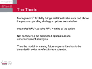
  • 6. The Thesis Managements‟ flexibility brings additional value over and above the passive operating strategy – options are valuable expanded NPV= passive NPV + value of the option Not considering the embedded options leads to underinvestment strategies Thus the model for valuing future opportunities has to be amended in order to reflect its true potential.
  • 7. The Research 1.Qualitative review of the related literature • Theoretical background • Specific application of ROA, with focus on the Telecommunication sector 2. Quantitative application of the models and techniques on a particular project - FTTH • Several types of Options • Option to differ the investment • Option to contract the investment • Growth option
  • 8. The Research cont‟d. • Different calculation methodologies • Closed form solution • Lattices • Simulation • Application of five different parameterizations for approximation of the diffusion process
  • 9. Qualitative - application of ROA Most extensive application of ROA in • Natural resources utilization – Oil and Mining sector • Pharmaceutical, specifically R & D Due to: • Capital intensity • Availability of traded assets – option • High uncertainty Application of ROA in Telecommunication sector: • With the beginning of deregulation of the sector and regulation Telecom operators with significant market power • Mostly for justification of costs and allowable investment base • Only recently for application of new technologies
  • 10. Qualitative - Required assumptions - cont‟d Conditions for application of Financial assets valuation tools to valuation of Real assets ROA is considered as an extension to the DCF/NPV analysis, not as a substitute hence: • average rational investor is a risk averse • prefers more to less wealth All option pricing models are based on the concept of riskless hedge and no arbitrage opportunities hence: • The market is complete - any state of the world can be replicated by some combination of the existing securities.
  • 11. Qualitative - Required assumptions - cont‟d • Complete market for Binomial - there are at least two linearly independent securities: • a twin security and a • riskless bond • Black - Scholes assumptions: • There are no transaction costs; • The investor may borrow any fraction of the purchase price at the short term risk free interest rate; • Short selling is permitted; • The call option can be exercised only on its expiration date; • Trading of securities takes place continuously; • The stock price (underlying asset) follows a geometric Brownian motion with constant drift and volatility, and • The underlying security does not pay dividends.
  • 12. Qualitative - Required assumptions - cont‟d The diffusion process – changes of the underlying asset value • Geometric Brownian motion - continuous stochastic process, with small random movements • Pure jump process, each successive asset price is almost the same as the previous price, but only occasionally with low probability of occurrence significantly different • Combination • It has to correspond to the actual asset being analyzed
  • 13. Qualitative - Required assumptions - cont‟d Incomplete market - partially solved by so called the integrated – two risks type approach The additional assumptions / conditions for this so called “Partially complete market” are: • Securities depend only on market states, • The market is complete with respect to the market uncertainties and • Private events convey no information about future market events. Disaggregation of uncertainties Drawback: Private and Market uncertainties might be correlated
  • 14. Qualitative – Option valuation techniques Categorized in three broader valuation techniques: 1. Partial differential equations - Black – Scholes as a closed – form solution - Analytical approximations - Numerical methods, such as finite difference method 2. Simulations - Monte Carlo 3. Lattices - Binomial - Trinomial - Quadrinomial - Multinomial
  • 15. Options Strike or Exercise price Price of underlying asset Net Payoff Out-of-the-money In-the-money At-the-money Strike or Exercise price Price of underlying asset Net Payoff In-the-money Out-of-the-money At-the-money Payoff of Call Option Payoff of Put Option
  • 16. Qualitative - Option valuation techniques Black – Scholes as a closed – form solution Where C is the value of the call option S0 is the current value of the underlying asset; X is the cost of investing or strike price; r risk free rate of return; T is the time to expiration or validity of the real option; N(d1) and N(d2) are values from normal standard distribution is the volatility r is the risk-free rate 𝐶 = 𝑁 𝑑1 𝑆0 − 𝑁 𝑑2 𝑋𝑒−𝑟𝑇 𝑑1 = 𝑙𝑛 𝑆𝑜 𝑋 + 𝑟 + 𝜎2 2 𝑇 𝜎 𝑇 𝑑2 = 𝑑1 − 𝜎 𝑇 0 0.2 0.4 0.6 0.8 1 1.2 -3.00 -2.50 -2.00 -1.50 -1.00 -0.50 0.00 0.50 1.00 1.50 2.00 2.50 3.00
  • 17. Qualitative - Option valuation techniques Simulations is the volatility St and St-1 are the values of the underlying asset at time t and t-1 t is the time increment r is the risk free rate of return is value from normal standard distribution with mean zero and a variance of 1.0. 𝑆𝑡 = 𝑆𝑡−1 + 𝑆𝑡−1(𝑟 𝛿𝑡 + 𝜎𝜀 𝛿𝑡) 𝑚𝑎𝑥 𝑆𝑡 − 𝑋, 0 -1.50 -1.00 -0.50 0.00 0.50 1.00 1.50 0 0.2 0.4 0.6 0.8 1 1.2Time Wiener Process Z w/o Drift +STDEV(Z)= +SQRT(T) -STDEV(Z)=- SQRT(T)
  • 18. Qualitative - Option valuation techniques Lattices – Binomial 𝑢 = 𝑒(𝜎 𝛿𝑡) 𝑑 = 𝑒−(𝜎 𝛿𝑡) 𝑝 = 𝑒(𝑟𝛿𝑡 ) − 𝑑 𝑢 − 𝑑 𝛿𝑡 = 𝑇 𝑛 𝐶 = 𝑛! 𝑗! 𝑛 − 𝑗 ! 𝑛 𝑗=0 𝑝 𝑗 1 − 𝑝 𝑛−𝑗 𝑚𝑎𝑥 0, 𝑢 𝑗 𝑑 𝑛−𝑗 𝑆0 − 𝑋 𝑒 𝑟𝛿𝑡 𝑝 = 𝑒(𝑟−𝑦)𝛿𝑡 −𝑑 𝑢−𝑑 S0 S0u S0d S0u2 S0ud S0d2 S0u3 1/8 S0u2d 3/8 S0du2 3/8 S0d3 1/8 0 1 2 3 Time increments
  • 19. Qualitative Option valuation techniques Lattices – Qudrinomial S0 S0u1u2 S0u1d2 S0u12u2d2 S0u12u22 S0u1u2d1d2 S0u1d1u22 S0u12d22 S0u12u2d2 S0u1d1d22 S0u1u2d1d2 S0d1u2 S0d1d2 S0u1u2d1d2 S0u1d1u22 S0d12u2d2 S0d12u22 S0u1d1d22 S0u1d1u2d2 S0d12d22 S0 d12u2d2
  • 20. Qualitative research – Integration of DTA S0 S0 u S0 udx1 S0 u 2 x1 S0 udy1 S0 u 2 y1 S0 d S0 d 2 x1 S0 udx1 S0 d 2 y1 S0 udy1 p p1 (1-p) p1 p(1-p1 ) (1-p)(1-p1 ) p p1 (1-p) p1 p(1-p1 ) (1-p)(1-p1 ) Where x1 and y1 are asset correction factors
  • 22. Quantitative - FTTH DCF FTTH DCF Analysis Year 0 1 2 3 4 5 6 FTTH Residential & Business Fast Internet customers - new sales100% 8700 20000 28000 44000 10000 6000 WS participation in total sales 10% 20% 20% 20% 20% Distribution of FTTH Fast Internet customers Residential 59% 50% 50% 50% 50% 50% Residential +HD TV 32% 41% 41% 41% 41% 41% Business 10% 10% 10% 10% 10% 10% FTTH incremental monthly fee Residential monthly fee - FTTH Fast Internet € 4,5 € 4,2 € 3,9 € 3,9 € 3,9 € 3,9 Residential monthly fee - FTTH Fast Internet and HD TV € 10,0 € 9,3 € 8,6 € 8,6 € 8,6 € 8,6 Business monthly fee - FTTH Fast Internet € 11,0 € 10,2 € 9,5 € 9,5 € 9,5 € 9,5 Average Rate Per User (ARPU) € 24,0 € 24,0 € 23,0 € 22,0 € 22,0 € 22,0 Revenues Residential monthly fee - FTTH Fast Internet € 137.417 € 464.861 € 781.585 € 1.149.390 € 1.126.402 € 367.805 Residential monthly fee - FTTH Fast Internet and HD TV € 164.430 € 845.203 € 1.421.064 € 2.089.800 € 2.048.004 € 668.736 Business monthly fee - FTTH Fast Internet € 57.420 € 229.561 € 385.968 € 567.600 € 556.248 € 181.632 ARPU revenues € 1.252.800 € 5.385.600 € 11.785.200 € 20.776.800 € 27.904.800 € 30.808.800 Total Revenues € 1.612.067 € 6.925.225 € 14.373.817 € 24.583.590 € 31.635.454 € 32.026.973 Cost margin as % of sales 50% 40% 39% 38% 37% 36% Total operating costs € 806.033 € 2.770.090 € 5.605.789 € 9.341.764 € 11.705.118 € 11.529.710 EBITDA € 806.033 € 4.155.135 € 8.768.028 € 15.241.826 € 19.930.336 € 20.497.263 Depreciation € 1.089.866 € 2.858.296 € 4.950.663 € 6.670.126 € 6.399.402 € 5.556.420 EBIT -€ 283.833 € 1.296.839 € 3.817.366 € 8.571.700 € 13.530.934 € 14.940.842 Tax @ 10% 10% € 0 € 129.684 € 381.737 € 857.170 € 1.353.093 € 1.494.084 Net income -€ 283.833 € 1.167.155 € 3.435.629 € 7.714.530 € 12.177.841 € 13.446.758 Operating cash flow (CF) € 806.033 € 4.025.451 € 8.386.292 € 14.384.656 € 18.577.243 € 19.003.178 Present value (PV) CF @ 13.6% WACC € 709.536 € 3.119.305 € 5.720.513 € 8.637.462 € 9.819.505 € 8.842.117 CF PV cumulative € 709.536 € 3.828.842 € 9.549.355 € 18.186.817 € 28.006.322 € 36.848.439 Capital expenditures (CAPEX) € 7.933.494 € 10.055.587 € 12.351.415 € 8.046.443 € 3.283.084 € 2.236.696 € 0 CAPEX PV @ 13.6% WACC € 7.933.494 € 8.851.749 € 9.571.060 € 5.488.693 € 1.971.373 € 1.182.267 € 0 Total CAPEX PV € 34.998.635 CF PV cummulative - CAPEX PV cummulative -€ 34.998.635 -€ 34.289.099 -€ 31.169.793 -€ 25.449.280 -€ 16.811.818 -€ 6.992.313 € 1.849.804 Net Present Value (NPV) as of Y6 € 1.849.804 Discounted payback period (Years) 5,79 Internal rate of return (IRR) 15,79%
  • 23. Quantitative FTTH input estimates Method annual volatility in % Implied volatility B-S model 27.47 Logarithmic CF from project returns 29.70 Logarithmic stock price returns 30.91 Standard deviation in firm value1 40.64 Inputs Date Stock price € 8,68 05.03.2012 Dividend € 0,70 Dividend yield 8,06% Call option value 0,9 05.03.2012 Exercise price 8 21.06.2013 Risk - free rate (annual) dis. 0,13% Risk - free rate (annual) con. 0,13% Black Scholes calculator INPUTS OUTPUTS Standard deviation (annual) 27,47% d1 0,088264 Maturity (in years) 1,30 d2 -0,22446 Risk - free rate (annual) 0,13% N(d1) 0,535167 Stock price € 8,68 N(d2) 0,4112 Exercise price € 8,00 B-S call 0,900052 Divident yield (annual) 8% B-S put 1,068341 12 23.01.2012-27.01.2012 511 -0,004 8,50322E-07 13 16.01.2012-20.01.2012 513 -0,004 8,78585E-07 14 09.01.2012-13.01.2012 515 -0,002 8,34354E-06 15 03.01.2012-05.01.2012 516 -0,008 8,37328E-06 16 26.12.2011-29.12.2011 520 0,000 2,33133E-05 17 19.12.2011-23.12.2011 520 -0,010 2,24777E-05 18 12.12.2011-16.12.2011 525 0,006 0,000111494 19 05.12.2011-09.12.2011 522 -0,015 0,000107766 20 28.11.2011-02.12.2011 530 0,019 0,000570091 21 21.11.2011-25.11.2011 520 0,016 0,000413413 22 14.11.2011-18.11.2011 512 0,010 0,000214388 23 07.11.2011-11.11.2011 507 0,002 4,6277E-05 24 31.10.2011-04.11.2011 506 0,002 4,63301E-05 25 24.10.2011-28.10.2011 505 0,000 2,33133E-05 26 17.10.2011-21.10.2011 505 0,000 2,33133E-05 27 10.10.2011-14.10.2011 505 0,000 2,33133E-05 28 03.10.2011-07.10.2011 505 -0,002 8,12332E-06 29 26.09.2011-30.09.2011 506 -0,004 7,80759E-07 30 19.09.2011-23.09.2011 508 0,006 0,000115593 31 12.09.2011-16.09.2011 505 -0,010 2,52397E-05 32 05.09.2011-09.09.2011 510 -0,004 8,36282E-07 33 29.08.2011-02.09.2011 512 0,004 7,64275E-05 34 22.08.2011-26.08.2011 510 0,016 0,000425968 35 15.08.2011-19.08.2011 502 -0,006 1,27673E-06 36 08.08.2011-12.08.2011 505 0,006 0,000116353 37 01.08.2011-05.08.2011 502 0,002 4,65452E-05 38 25.07.2011-29.07.2011 501 0,000 2,33133E-05 39 18.07.2011-22.07.2011 501 0,000 2,33133E-05 40 11.07.2011-15.07.2011 501 -0,004 7,12868E-07 41 04.07.2011-08.07.2011 503 0,006 0,000116866 42 27.06.2011-01.07.2011 500 0,000 2,33133E-05 43 20.06.2011-24.06.2011 500 -0,002 8,01106E-06 44 13.06.2011-17.06.2011 501 -0,002 8,03363E-06 45 06.06.2011-09.06.2011 502 -0,006 1,27673E-06 46 30.05.2011-03.06.2011 505 0,012 0,000281592 47 23.05.2011-27.05.2011 499 0,018 0,000530339 48 16.05.2011-20.05.2011 490 -0,002 7,78213E-06 49 09.05.2011-13.05.2011 491 -0,008 1,07929E-05 50 03.05.2011-06.05.2011 495 0,031 0,001267363 51 26.04.2011-29.04.2011 480 0,043 0,002245622 52 18.04.2011-21.04.2011 460 -0,264 0,067188126 53 11.04.2011-15.04.2011 599 / / Average -0,005 Total 0,101483 4,46% 30,91% Weekly volatility Yearly volatility
  • 24. Quantitative – Option to defer Step 0 1 Factors u= 1,362 d= 0,734 p= 0,524 44,19 Sou e 32,44 8,69 So k 4,28 23,81 Sod k 0,00 Related decision e - exercise the option k- keep the option 𝑉 = 𝑝 𝑚𝑎𝑥 0, 𝑢 𝑆0 − 𝑋 + 1 − 𝑝 𝑚𝑎𝑥 0, 𝑑 𝑆0 − 𝑋 𝑒 𝑟𝛿𝑡 The input parameters (in million €) are as follows: Stock price (PV of the cash flow as of now) S0= 32.4 Exercise price (PV of the investment as of Year 1) X=35.5 Standard deviation (annual volatility of the asset) =30.9% Risk-free rate (continuous) rf=6.1% Time to expiration T=1 Year Time step t=1 BS yields 3.58 million € Simulation yields 3.98 million €
  • 25. Quantitative – Option to defer Step 0 1 2 3 4 5 Factors 64,75 u= 1,148 Sou5 e d= 0,871 56,39 29,25 p= 0,510 Sou4 k 49,11 21,32 49,11 Sou3 k Sou4 d e 14,47 42,77 13,61 42,77 Sou3 d k Sou2 k 37 7,70 37,25 37,25 9,37 Sou2 d k Sou3 d2 e Sou k 4,30 1,75 32,44 5,87 32,44 32,44 So k Soud k Sou2 d2 k 3,59 28,25 2,38 0,88 Sod k 28,25 28,25 1,31 24,60 Soud2 k Sou2 d3 k Sod2 k 0,44 24,60 0,00 0 Soud3 k Related decision 21 0,00 21,43 e - exercise the option Sod3 k Soud4 k k- keep the option 0 19 0,00 Sod4 k 0,00 16,25 Sod5 k 0,00
  • 26. Quantitative Method Annual volatility in Binomial 1 step Binomial 5 steps B-S model Standard deviation in firm value 40,64 5,90 4,95 4,84 Logarithmic stock price returns 30,91 4,28 3,59 3,58 Logarithmic CF from project returns 29,70 4,07 3,59 3,58 Implied volatility B-S model 27,47 3,69 3,42 3,43 Option value in 1.000.000 EUR The option value is highly sensitive to the time step and the volatility
  • 27. Quantitative Different parameterizations Trigeorgis 𝜇 = 𝛼 𝜎2 − 1 2 (23) 𝑘 = 𝜎 𝛿𝑡 (24) ℎ = 𝑘2 + (𝑘2 𝜇)2 (25) 𝑝 = 1 2 (1 + 𝑘2 𝜇 ℎ ) (26) 𝜇 = 𝛼 𝜎2 − 1 2 (23) 𝑘 = 𝜎 𝛿𝑡 (24) ℎ = 𝑘2 + (𝑘2 𝜇)2 (25) 𝑝 = 1 2 (1 + 𝑘2 𝜇 ℎ ) (26) 𝑢 = 𝑒 𝑟− 𝜎2 2 𝛿𝑡+𝜎 𝛿𝑡 (27) 𝑑 = 𝑒 𝑟− 𝜎2 2 𝛿𝑡−𝜎 𝛿𝑡 (28) 𝑢𝑑 = 𝑒 2 𝑟− 𝜎2 2 𝛿𝑡 (29) 𝑢 = 𝑒 𝑟− 𝜎2 2 𝛿𝑡+𝜎 𝛿𝑡 (27) 𝑑 = 𝑒 𝑟− 𝜎2 2 𝛿𝑡−𝜎 𝛿𝑡 (28) 𝑢𝑑 = 𝑒 2 𝑟− 𝜎2 2 𝛿𝑡 (29) = r- 𝑢 = 𝑒ℎ , 𝑑 = 𝑒−ℎ 𝑒 𝜎2 𝛿𝑡 − 1𝑢 = 𝑒 𝑒 𝜎2 𝛿𝑡 −1+𝑟𝛿𝑡 𝑑 = 𝑒− 𝑒 𝜎2 𝛿𝑡 −1+𝑟𝛿𝑡 𝑝 = 𝑒 𝑟𝛿𝑡 − 𝑑 𝑢 − 𝑑 Rendelmann – Bartter Hull 𝑝 = 1 2 𝜎 𝛿𝑡 Haahtela
  • 28. Quantitative Different parameterizations 0,00 0,50 1,00 1,50 2,00 2,50 3,00 3,50 4,00 4,50 5,00 1 2 5 10 Project value [millionEUR] number of steps n BS CRR RB Trigerogis Hull Haahtela =30,9% Option to defer the investment for one year
  • 29. Quantitative Different parameterizations -1 0 1 2 3 4 5 6 0% 5% 10% 15% 20% 25% 30% 35% 40% 45% Project value [million €] Volatility BS CRR Trigeorgis RB Hull Haahtela 0 0.5 1 1.5 2 5% 10% 15% 20% Option to Differ the Investment (Double Step) With Different Parameterizations in Relation to Volatility
  • 30. Quantitative Different parameterizations Method Annual volatility in % BS model in 1.000.000 EUR CRR 1 step RB 1 step Trigerogis 1 step Hull 1 step Haahtela 1 step Standard deviation in firm value 40,64 4,8347 22,07 18,38 21,92 27,93 32,23 Logarithmic stock price returns 30,91 3,5818 19,47 21,86 19,17 23,05 30,92 Logarithmic CF from project returns 29,70 3,4251 18,90 22,27 18,71 22,24 30,83 Implied volatility B-S model 27,47 3,1371 17,55 22,98 17,68 20,46 30,66 Assumed volatility 20,00 2,1707 8,32 25,29 11,57 10,04 30,59 Assumed volatility 10,00 0,8889 -70,76 27,97 -30,71 -70,04 31,59 Assumed volatility 7,00 0,5184 -100,00 26,27 -94,02 -100,00 30,04 17,26 22,16 17,81 20,74 31,04 5,26 2,50 3,83 6,59 0,68Standard deviation of higher (20% and above) volatilities Average of higher (20% and above) volatilities Relative error between different parameterizations and B-S as reference in % Method Annual volatility in % BS model in 1.000.000 EUR CRR 2 steps RB 2 steps Trigerogis 2 steps Hull 2 steps Haahtela 2 steps Standard deviation in firm value 40,64 4,8347 0,00 1,70 -0,13 -2,05 5,89 Logarithmic stock price returns 30,91 3,5818 2,94 1,09 2,72 -4,19 5,54 Logarithmic CF from project returns 29,70 3,4251 3,40 1,04 3,21 -4,56 5,42 Implied volatility B-S model 27,47 3,1371 4,29 0,97 4,22 -5,31 5,16 Assumed volatility 20,00 2,1707 7,69 1,28 8,71 -8,29 3,50 Assumed volatility 10,00 0,8889 -2,82 6,41 12,45 2,56 -4,06 Assumed volatility 7,00 0,5184 -63,46 12,37 -7,57 63,23 -10,99 3,67 1,21 3,75 -4,88 5,10 2,77 0,29 3,21 2,26 0,93 Average of higher (20% and above) volatilities Standard deviation of higher (20% and above) volatilities Relative error between different parameterizations and B-S as reference in % Single step Double step
  • 31. Quantitative Different parameterizations Five step Ten step Method Annual volatility in % BS model in 1.000.000 EUR CRR 5 step RB 5 step Trigerogis 5 step Hull 5 step Haahtela 5 step Standard deviation in firm value 40,64 4,8347 2,40 0,56 2,35 3,36 6,09 Logarithmic stock price returns 30,91 3,5818 0,25 1,71 0,16 0,83 5,72 Logarithmic CF from project returns 29,70 3,4251 -0,20 1,82 -0,27 0,35 5,67 Implied volatility B-S model 27,47 3,1371 -1,19 1,99 -1,21 -0,71 5,58 Assumed volatility 20,00 2,1707 -7,28 2,23 -6,98 -7,09 5,09 Assumed volatility 10,00 0,8889 0,18 -1,18 4,89 0,26 1,39 Assumed volatility 7,00 0,5184 -23,24 -8,43 -5,48 -23,17 -6,02 -1,20 1,66 -1,19 -0,65 5,63 Standard deviation of higher (20% and above) volatilities 3,64 0,65 3,49 3,90 0,36 Relative error between different parameterizations and B- S as reference in % Average of higher (20% and above) volatilities Method Annual volatility in % BS model in 1.000.000 EUR CRR 10 step RB 10 step Trigerogis 10 step Hull 10 step Haahtela 10 step Standard deviation in firm value 40,64 4,8347 2,02 2,23 1,99 2,47 -0,16 Logarithmic stock price returns 30,91 3,5818 2,46 2,29 2,42 2,74 0,23 Logarithmic CF from project returns 29,70 3,4251 2,48 2,30 2,45 2,74 0,31 Implied volatility B-S model 27,47 3,1371 2,47 2,32 2,45 2,69 0,47 Assumed volatility 20,00 2,1707 1,20 2,52 1,42 1,33 1,27 Assumed volatility 10,00 0,8889 -0,19 3,38 1,97 -0,16 3,43 Assumed volatility 7,00 0,5184 -11,94 2,53 -6,25 -11,93 3,28 2,13 2,33 2,15 2,39 0,42 Standard deviation of higher (20% and above) volatilities 0,56 0,11 0,45 0,61 0,52 Average of higher (20% and above) volatilities Relative error between different parameterizations and BS as reference in %
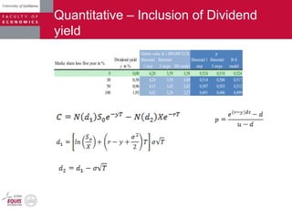
  • 32. Quantitative – Inclusion of Dividend yield Marke share loss first year in % Dividend yield y in % Binomial 1 step Binomial 5 steps BS model Binomial 1 step Binomial 5 steps B-S model 0 0,00 4,28 3,59 3,58 0,524 0,510 0,524 30 0,58 4,20 3,50 3,49 0,514 0,506 0,517 50 0,96 4,15 3,43 3,42 0,507 0,503 0,512 100 1,93 4,02 3,28 3,27 0,491 0,496 0,499 Option value in 1.000.000 EUR p
  • 33. Quantitative – Integration of DTA into ROA S0 S0 u S0 udx1 S0 u 2 x1 S0 udy1 S0 u 2 y1 S0 d S0 d 2 x1 S0 udx1 S0 d 2 y1 S0 udy1 p p1 (1-p) p1 p(1-p1 ) (1-p)(1-p1 ) p p1 (1-p) p1 p(1-p1 ) (1-p)(1-p1 ) Step 0 1 2 Factors u= 1,362 61,25 d= 0,734 Sou2 x1 e p= 0,524 25,75 p1= 0,100 x1= 1,02 33,01 y1= 1,00 Soudx1 k 44,19 0,00 Sou k 12,22 60,19 Sou2 y1 e 24,69 32,44 Soudy1 k 0,00 32,44 So k 6,02 33,01 Soudx1 k 0,00 17,79 Sod2 x1 k 23,81 0,00 Sod k 0,00 32,44 Soudy1 k 0,00 Related decision 17,48 e - exercise the option Sod2 y1 k k- keep the option 0,00
  • 34. Quantitative – Option to contract The input parameters (in million €) are as follows: Stock price (PV of the cash flow as of now) S0= 36.85 Savings from contraction cs=16.24 Contraction factor cf = 50% Standard deviation (annual volatility of the asset) =30.9% Risk-free rate (continuous) rf=6.1% Time to expiration T=3 Year Time step t=1 Step 0 1 2 3 Factors u= 1,362 d= 0,734 p= 0,524 93,14 Sou3 k 93,14 68,38 Sou2 k 50 50,19 68,38 Sou2 d k Sou e 50,19 36,85 50,74 36,85 So e Soud e 38,65 27,05 38,06 Sod e 27,05 30,48 19,86 Soud2 e Sod2 e 29,76 26,17 Related decision 15 e - exercise the option Sod3 e k- keep the option 23,53 Binomial Vo=1,8 million € B-S Vo=1,45 million €
  • 35. Quantitative – Sequential compound Inter-project compoudness Option on option Stock price (PV of the cash flow as of now) S0= 36.85 Exercise prices X5= 2.24 X4= 3.28 X3= 8.05 X2= 12.35 X1= 10.06 X0= 7.93 Standard deviation (annual volatility of the asset) =30.9% Risk-free rate (continuous) rf=6.1% Time to expiration T=6 Year Time step t=1
  • 36. Quantitative – Sequential compound Step 0 1 2 3 4 5 6 235,43 Factors 172,83 Sou6 e u= 1,362 Sou5 e 233,19 d= 0,734 126,88 170,59 p= 0,524 Sou4 e 126,88 X5= 2,237 93,14 124,83 93,14 Sou5 d e Sou3 e Sou4 d e 124,64 91,25 68,38 91,04 68,38 Sou3 d e 68,38 Sou2 e 50 66,40 50,19 Sou4 d2 e 50,19 68,38 Sou2 d e Sou3 d2 e 66,14 Sou e 48,33 48,09 36,85 50,19 36,85 36,85 36,85 So e Soud e Sou2 d2 e Sou3 d3 36,50 27,05 36,85 34,87 34,61 Sod e 27,05 27,05 26,27 19,86 Soud2 e Sou2 d3 e 19,86 Sod2 e 25,19 19,86 24,95 Sou2 d4 e 18,11 Soud3 e 17,62 15 17,88 14,58 Sod3 e Soud4 e 10,70 13 11 12,47 Soud5 e Sod4 e 8,47 8,72 7,86 Related decision Sod5 e 5,77 e - exercise the option 5,75 Sod5 e k- keep the option 3,53
  • 37. Quantitative – Sequential compound Step 0 1 2 3 4 5 Factors 170,73 u= 1,362 Sou5 e d= 0,734 124,90 167,44 p= 0,524 Sou4 e X4= 3,283 91,28 121,81 91,04 Sou3 e Sou4 d e 88,37 66,40 87,75 68,38 Sou3 d e Sou2 e 48,33 63,31 48,09 50,19 65,09 Sou2 d e Sou3 d2 e Sou e 45,43 44,81 36,50 47,11 36,85 34,87 So e Soud e Sou2 d2 e 33,99 26,27 33,57 31,78 Sod e 25,19 24,95 24,06 18,11 Soud2 e Sou2 d3 e Sod2 e 22,28 17,88 21,66 16,80 Soud3 e 12,72 14,79 12,47 Sod3 e Soud4 e 9,81 8,72 9,19 Sod4 e 5,63 5,75 Related decision Sod5 e e - exercise the option 2,47 k- keep the option Asset values are replaced by option values from previous lattice
  • 38. Quantitative – Sequential compound Step 0 1 2 3 4 X3= 8,046 121,81 Sou4 e 88,37 113,76 Sou3 e 80,80 63,31 65,09 Sou3 d e Sou2 e 45,43 55,26 47,11 57,05 Sou2 d e Sou e 37,86 33,99 39,54 33,57 31,78 So e Soud e Sou2 d2 e 26,87 24,06 25,52 23,73 Sod e 22,28 16,50 16,80 Soud2 e Sod2 e 14,71 14,79 8,76 Soud3 e 9,81 6,74 Sod3 e 3,32 5,63 Sod4 k 0,00 Related decision e - exercise the option k- keep the option
  • 39. Quantitative – Sequential compound Step 0 1 2 3 4 X3= 8,046 121,81 Sou4 e 88,37 113,76 Sou3 e 80,80 63,31 65,09 Sou3 d e Sou2 e 45,43 55,26 47,11 57,05 Sou2 d e Sou e 37,86 33,99 39,54 33,57 31,78 So e Soud e Sou2 d2 e 26,87 24,06 25,52 23,73 Sod e 22,28 16,50 16,80 Soud2 e Sod2 e 14,71 14,79 8,76 Soud3 e 9,81 6,74 Sod3 e 3,32 5,63 Sod4 k 0,00 Related decision e - exercise the option k- keep the option
  • 40. Quantitative – Sequential compound Step 0 1 2 3 X2= 12,351 80,80 Sou3 e 68,45 57,05 Sou2 e 37,86 39,54 45,15 Sou2 d e Sou e 25,51 26,87 28,35 25,52 So e Soud e 17,20 16,50 13,62 Sod e 14,71 7,23 8,76 Soud2 e Sod2 e 2,36 1,16 Related decision 3,32 e - exercise the option Sod3 k k- keep the option 0,00
  • 41. Quantitative – Sequential compound Step 0 1 2 X1= 10,056 45,15 Sou2 e 28,35 35,09 Sou e 17,20 18,89 13,62 So e Soud e 10,09 7,23 3,57 Sod e Related decision 1,76 1,16 e - exercise the option Sod2 k k- keep the option 0,00 Step 0 1 X0= 7,933 18,89 Sou e 10,09 10,95 So e 5,40 1,76 Sod k Related decision 0,00 e - exercise the option k- keep the option
  • 42. Quantitative – Sequential compound Option / project values taken from related lattice Step 0 1 2 3 4 5 6 Sou6 Sou5 233,19 167,44 Sou4 113,76 Sou5 d Sou3 Sou4 d 124,64 68,45 87,75 Sou3 d Sou2 55,26 Sou4 d2 35,09 Sou2 d Sou3 d2 66,14 Sou 25,51 44,81 10,95 So Soud Sou2 d2 Sou3 d3 5,40 3,57 23,73 34,61 Sod 0,00 Soud2 Sou2 d3 Sod2 2,36 21,66 Sou2 d4 0,00 Soud3 17,62 6,74 Sod3 Soud4 0,00 9,19 Soud5 Sod4 8,47 0,00 Sod5 2,47 Sod5 3,53
  • 43. Quantitative – Changing volatilities Stock price (PV of the cash flow as of now) S0= 28.55 Exercise price (PV of CAPEX as of Y2) X=43.10 Standard deviation (annual Volatility year 1) =40.64% Standard deviation (annual Volatility year 2) =30.91% Risk-free rate (continuous yearly) rf=6.1% Time to expiration T=2 Years Time step t=1 Step 0 1 2 Factors u1= 1,501 58 d1= 0,666 Sou1u2 e p1= 0,475 15,29 43 u2= 1,362 Sou1 k d2= 0,734 7,53 p2= 0,524 31 Sou1d2 k 0,00 28,55 So k 3,37 26 Sod1u2 k 0,00 19 Sod1 k 0,00 Related decision 14 e - exercise the option Sod1d2 k k- keep the option 0,00 r 2 = 2 + 2
  • 44. Quantitative – Different volatilities r 2 = 2 + 2 Stock price (PV of the cash flow as of now) S0= 28.55 Exercise price (PV of CAPEX as of Y2) X=43.10 Standard deviation (annual Volatility year 1) =74.17% Standard deviation (annual Volatility year 2) =30.91% Risk-free rate (continuous yearly) rf=6.1% Time to expiration T=2 Years Time step t=1 Step 0 1 2 Factors 234 u1= 1,362 Sou1u2u1u2 d1= 0,734 190 p1= 0,524 53 82 Sou1u2u1d2 u2= 2,100 Sou1u2 10 d2= 0,476 50 50 126 p2= 0,361 Sou1u2d1u2 83 29 Sou1u2d1d2 0 53 Sou1d2u1u2 10 12 19 Sou1d2u1d2 Sou1d2 0 2 2 29 Sou1d2d1u2 0 6 Sou1d2d1d2 28,55 0 So 13 13 126 Sod1u2u1u2 83 29 44 Sod1u2u1d2 Sod1u2 0 19 19 68 Sod1u2d1u2 25 15 Sod1u2d1d2 0 29 Sod1d2u1u2 0 6 10 Sod1d2u1d2 Sod1d2 0 0 0 15 Sod1d2d1u2 0 3 Sod1d2d1d2 0 Vp=12.6 million € r=80.35% VBS = 9.96 million €
  • 45. Summary of the results 1. Average Average Method Annual volatility in % Passive NPV Option Value Expanded NPV Option Value Expanded NPV Option Value Expanded NPV Option Value Expanded NPV Option value Expanded NPV Standard deviation in firm value 40,64 1,85 2,98 4,83 4,05 5,90 3,10 4,95 2,90 4,75 3,26 5,11 Logarithmic stock price returns 30,91 1,85 1,73 3,58 2,43 4,28 1,74 3,59 2,13 3,98 2,01 3,86 Logarithmic CF from project returns 29,70 1,85 1,58 3,43 2,22 4,07 1,57 3,42 1,39 3,24 1,69 3,54 Implied volatility B-S model 27,47 1,85 1,29 3,14 1,84 3,69 1,25 3,10 1,32 3,17 1,42 3,27 Logarithmic stock price returns 30,91 1,85 1,42 3,27 2,17 4,02 1,43 3,28 1,12 2,97 1,54 3,39 2. Average Method Annual volatility in % Passive NPV Option Value Expanded NPV Option value Expanded NPV Logarithmic stock price returns 30,91 1,85 4,17 6,02 4,17 6,02 3. Average Average Method Annual volatility in % Passive NPV Option Value Expanded NPV Option Value Expanded NPV Option value Expanded NPV Logarithmic stock price returns 30,91 1,85 1,45 3,30 1,80 3,65 1,63 3,48 4. Average Method Annual volatility in % Passive NPV Option Value Expanded NPV Option value Expanded NPV Logarithmic stock price returns 30,91 1,85 3,55 5,40 3,55 5,40 5. Average Method Annual volatility in % Passive NPV Option Value Expanded NPV Option value Expanded NPV Standard deviation in firm value 40,64 Logarithmic stock price returns 30,91 6. Average Average Method Annual volatility in % Passive NPV Option Value Expanded NPV Option Value Expanded NPV Option Value Expanded NPV Option value Expanded NPV Logarithmic stock price returns 74,17 Logarithmic stock price returns 30,91 r 2 = 1 2 + 2 2 80,35 1,85 8,11 9,96 8,55 10,40 8,33 10,18 CRR 1 step CRR 5 steps CRR 3 stepsB-S Sequential compound option in 1.000.000 EUR Simulation Option to differ the investment for two years with private risks in 1.000.000 EUR Option to differ the investment for one year with competition inclouded (dividend yield y=1,93%) in 1.000.000 EUR CRR 1 step + DTA Option to contract the investment in the following three years in 1.000.000 EUR B-S CRR 2 steps Calculation model Option to differ the investment for one year in 1.000.000 EUR 1,52 3,37 CRR 6 steps Option to differ the investment for two years with changing volatilities in 1.000.000 EUR CRR 2 steps B-S 3,37 12,60 1,52 10,75 Option to differ the investment for two years with differnet volatilities in 1.000.000 EUR non recomb. 2 steps 1,85 1,85 10,75 12,60
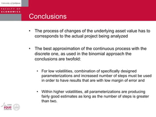
  • 46. Conclusions • Future management response to altered future business environment conditions expands an investment opportunity value by improving its upside potential or by limiting its downside losses, relative to the passive operating strategy • Related to the parameterizations conclusions are twofold: • For low volatilities, combination of specifically designed parameterizations and increased number of steps must be used in order to have results that are with low margin of error and • Within higher volatilities, all parameterizations are producing fairly good estimates as long as the number of steps is greater than two.
  • 47. Conclusions • The process of changes of the underlying asset value has to corresponds to the actual project being analyzed • The best approximation of the continuous process with the discrete one, as used in the binomial approach the conclusions are twofold: • For low volatilities, combination of specifically designed parameterizations and increased number of steps must be used in order to have results that are with low margin of error and • Within higher volatilities, all parameterizations are producing fairly good estimates as long as the number of steps is greater than two.
  • 49. Back up slide - Brownian motion & Jump