1. Carrying capacity of air environment
Er. Sunil Kumar Meena
MTech (Biochem Engg), MTech (Env Engg)
Scientist-E/Additional Director
Central Pollution Control Board
Regional Directorate, Bhopal
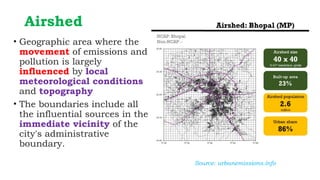
2. Airshed
• Geographic area where the
movement of emissions and
pollution is largely
influenced by local
meteorological conditions
and topography
• The boundaries include all
the influential sources in the
immediate vicinity of the
city's administrative
boundary.
Source: urbanemissions.info
3. Airshed delineation
Quantification of emissions to prepare a multi
pollutant emission inventory
Predicting air quality level using AQ modelling tools,
helps in understanding atmospheric transport of
pollutants from source to receptor and its dispersion in
the study area.
Collection of representative meteorological data & its
analysis to evaluate variations at local and regional
level
Delineating an airshed includes 03 main steps:
4. Assimilative capacity of an Airshed
Assimilative capacity of air environment is
the maximum amount of pollution load that
can be discharged into it without violating
the prescribed Ambient Air Quality standard.
The phenomena governing the assimilative
capacity of air environment include dilution,
dispersion and deposition.
Pollutants Industrial. Residential, Rural and Other areas
Concentration in µg/m3 (24 hourly) Concentration in µg/m3 (Annually)
SO2 80 50
NO2 80 40
PM10 100 60
PM2.5 60 40
5. Uses of Assimilative Capacity
It is an important tool for suggesting the
safe limits of disposal of pollutants for
industrial operations as well as for the area-
based management of air pollution and to
mitigate the pollution levels.
It is an indicator of potential for future growth
keeping in view the resources such as air, water,
land etc.
6. Estimation of assimilative capacity of an airshed
Second approach is based on Pollution Potential or Dispersion
potential
Assimilative capacity is inversely proportional to the pollution
potential and
directly proportional to the dispersion potential of the atmosphere.
It is estimated through dispersion models in terms of resulting ambient
air concentration of pollutants due to changes in the emission sources.
First approach is based on Ventilation Coefficient
Assimilative capacity of the atmosphere is directly proportional to the ventilation
coefficient, which is computed through meteorological parameters.
7. Ventilation coefficient is
expressed as a product of mixing
height (z) and average transport
wind speed (Uavg) within the
mixing layer.
It is an atmospheric condition
which gives an indication of the
air pollution dispersion, ambient
air quality and pollution
potential.
VC>6000 m2
/s – Effective dispersion
3000 m2
/s <VC<=6000 m2
/s – Moderate dispersion
VC <=3000 m2
/s – Poor dispersion
8. Estimation of the ventilation coefficient
Assume that the ground level air
temperature is 150
C, while the normal
maximum surface temperature for that
month is 260
C. At an elevation of 100m
and 300m, the temperature is found to be
170
C and 210
C. The wind has a velocity of
2m/s at 10m. The wind exponent is 0.3.
Ventilation coefficient =
366.7 x 4.47 = 1639.15m2
/s
12. Second approach is based on Pollution Potential or Dispersion potential
Gaussian Dispersion
Model named
Industrial Source
Complex Short
Term (ISCST).
The model considers
emission from kiln
and disperse it under
the influence of
meteorology
Weather Research
Forecast (WRF) model
- Meteorological data
on hourly time basis.
This helps in
- Predicting Worst
Case scenario
- Identifying stability
class based on solar
radiation
14. Sr.
No.
Parameter Value
Type of Fuel Used Coal + Husk
A. Monitored at Port Hole Height (3.0 m)
1. Diameter of Stack, m 3.0
2. Flue Gas Velocity, m/s 3.0
3. Flue Gas Temp., K 350
4. Actual PM Concentration, mg/Nm3
273
5. Corrected PM Concentration at
17% O2, mg/Nm3
420
6. Normalized Flow Volume at 25C,
(Nm3
/day)
16,77,818
B. Calculated/Expected at the Stack Top (30.0 m) and used in
Modeling Exercise
1. Top Diameter (m) 1.0
2. Exit Flue Gas Velocity (m/s)
(corresponding to top diameter)
27.0
3. Exit Flue Gas Temperature (K) 350
4. Stack Height, (m) 30
5. Actual PM Emission Load, kg/day 458
6. Corrected PM Emission Load at
17% O2, kg/day
705
7. Actual PM Emission Rate, g/s 5.30
8. Corrected PM Emission Rate at
17% O2, g/s
8.16
9. Daily Operational Schedule 24 hrs Continuous
Basic data of brick kiln (FCBTK)
15. Case study : 103 Brick kilns operational in radial distance of 11 KMs
from the centre of Rajakhera village, Dholpur, Rajasthan
• Mixing height (
https://urbanemissions.info/blog-
pieces/india-meterology-bydistrict
/
)
Month
Weighted mixing
height in KMs
Jan 0.257
Feb 0.354
Mar 0.476
Apr 0.654
May 0.738
Jun 0.865
Jul 0.782
Aug 0.574
Sep 0.549
Oct 0.462
Nov 0.307
Dec 0.220
City CAAQMS/AOD ratio
of 2019
Jhind 1.08
Bhiwani 1.12
Agra 0.96
Muzaffarnagar 1.07
Sonipat 0.994
Bulandsahar 0.998
Total area – 380 SQKM
16. Month PM2.5
(MT/Month)
Ratio
PM10/PM2.5
PM10
(MT/Month)
January 15 1.4 21
February 13 1.34 17
March 11 1.93 21
April 15 2.63 39
May 18 2.63 47
June 17 2.86 49
July 13 1.68 22
August 8 1.28 10
September 8 1.32 11
October 14 1.37 19
November 15 1.18 18
December 13 1.2 16
Estimated Pollution Load
Month PM10
(MT/Month)
January 10
February 13
March 18
April 25
May 28
June 33
July 30
August 22
September 21
October 18
November 12
December 8
Total Assimilative capacity
Month PM10
(MT/Month)
January -11
February -4
March -3
April -14
May -19
June -16
July 8
August 12
September 10
October -1
November -6
December -8
Total Supportive capacity
2019 Particulates
contribution of single
brick kiln in Tons/day
No. of brick kilns operation needs
to be restricted w.r.t. the
supportive capacity available
Month Supportive capacity available
in MT w.r.t. PM10
January -11
0.705
-16
February -4 - 6
March -3 - 5
April -14 - 20
May -19 - 27
June -16 - 22
July 8 +12
August 12 +17
September 10 +15
October -1 - 2
November -6 - 8
December
17. Scenario 1- NW Sector Scenario 2- W-SW Sector
Dominant Wind Speed- 0.50-2.10 m/s Dominant Wind Speed- 0.50-2.10 m/s
Scenario 3- N-E Sector Scenario 4- All Directions
Dominant Wind Speed- 0.50-2.10 m/s Dominant Wind Speed- 0.50-2.10 m/s
Receptor Grid Points within 11 km x 11 km area keeping
Rajakhera Village as the centre (grid cell size of 0.5 km x 0.5
km)
18. Cumulative Impact of 103 Brick Kilns for Actual PM Emission Scenario (458 kg/day)
Dominant
Wind in
North-
West
Dominant
Wind in
West-
South
West
Dominant
Wind in
North-
East
Wind equally
distributed in
All Directions
19. Cumulative Impact of 103 Brick Kilns
Sr.
No.
PM Emissions /
Meteorological
Scenario
No. of
Brick
Kilns
likely
to
impact
PM Conc.
Range
based on
Isopleths
(µg/m3)
PM Conc. (µg/m3)
Min. Max. Avg.
1. Actual Emission Scenario (458 kg/d or 5.30 g/s)
a. North-West (N-W)
Sector
62 20-30 23 24 24
b. West-South West
(W-SW) Sector
21 10-20 9 18 13
c. North-East (N-E)
Sector
20 1-10 9 10 9
d. All Directions 103 1-10 3 5 4
2. Corrected Emission Scenario (705 kg/d or 8.16 g/s)
a. North-West (N-W)
Sector
62 30-45 35 37 36
b. West-South West
(W-SW) Sector
21 15-30 13 28 20
c. North-East (N-E)
Sector
20 1-15 14 16 15
d. All Directions 103 1-15 5 8 6
Predicted 24 hourly PM Concentrations Levels
in Rajakhera Village for Different Emission
and Met Scenario
Impact of Single Brick Kiln
Distance in
Downwind
Direction
PM Concentrations (µg/m3)
Actual Emission
Scenario (458 kg/d or
5.30 g/s)
Corrected Emission
Scenario (705 kg/d or
8.16 g/s)
N-W
Sector
Wind Flow
All
Directions
Wind Flow
N-W
Sector
Wind Flow
All
Directions
Wind Flow
500 m 2.32 0.01 3.62 0.02
1 km 1.28 001 3.18 002
1.5 km 0.99 0.01 2.10 0.02
2 km 0.84 0.01 1.37 0.01
2.5 km 0.59 0.01 1.13 0.01
3 km 0.47 0.01 1.06 0.01
5 km 0.40 0.00 0.66 0.01
10 km 0.36 0.00 0.56 0.00
Predicted 24 hourly PM
Concentration from Single Brick Kiln
at different Downwind Distances
20. Limitation
The absence of actual stack emission data for the brick kilns
Non-availability of the local meteorological data
Based on the supportive capacity estimation and the sensitivity
analysis outcomes; regulatory authority may take decision on the
month-wise restriction on the operation of the brick kilns situated
on the upwind direction i.e. North, North-West considering the
distance from the Rajakhera village.