4. 4
Algorithms
Definition: An algorithm is a finite sequence of
precise instructions for performing a computation
or for solving a problem.
Example: Describe an algorithm for finding the
maximum value in a finite sequence of integers.
Solution: Perform the following steps:
1. Set the temporary maximum equal to the first integer in the
sequence.
2. Compare the next integer in the sequence to the temporary
maximum.
If it is larger than the temporary maximum, set the temporary maximum
equal to this integer.
3. Repeat the previous step if there are more integers. If not, stop.
4. When the algorithm terminates, the temporary maximum is the
largest integer in the sequence.
5. 5
Specifying Algorithms
Algorithms can be specified in different ways. Their steps
can be described in English or in pseudocode.
Pseudocode is an intermediate step between an English
language description of the steps and a coding of these
steps using a programming language.
Pseudocode helps us analyze the time required to solve
a problem using an algorithm, independent of the actual
programming language used to implement algorithm.
6. 6
Properties of Algorithms
Input: An algorithm usually has input values from a specified set.
Output: From the input values, the algorithm produces the output
values from a specified set. The output values are the solution.
Correctness: An algorithm should produce the correct output
values for each set of input values.
Finiteness: An algorithm should produce the output after a finite
number of steps for any input.
Effectiveness: It must be possible to perform each step of the
algorithm correctly and in a finite amount of time.
Generality: The algorithm should work for all problems of the
desired form.
7. 7
Finding the Maximum Element in a Finite
Sequence
The algorithm in pseudocode:
Does this algorithm have all the properties
listed on the previous slide?
procedure max(a1, a2, …., an: integers)
max := a1
for i := 2 to n
if max < ai then max := ai
return max{max is the largest element}
8. 8
Some Example Algorithm Problems
Three classes of problems will be studied
in this section.
1. Searching Problems: finding the position of
a particular element in a list.
2. Sorting problems: putting the elements of a
list into increasing order.
3. Optimization Problems: determining the
optimal value (maximum or minimum) of a
particular quantity over all possible inputs.
9. 9
Searching Problems
Definition: The general searching problem is to
locate an element x in the list of distinct elements
a1,a2,...,an, or determine that it is not in the list.
The solution to a searching problem is the location of the
term in the list that equals x (that is, i is the solution if x
= ai) or 0 if x is not in the list.
For example, a library might want to check to see if a
patron is on a list of those with overdue books before
allowing him/her to checkout another book.
We will study two different searching algorithms; linear
search and binary search.
10. 10
Linear Search Algorithm
The linear search algorithm locates an item in a list by examining elements
in the sequence one at a time, starting at the beginning.
First compare x with a1. If they are equal, return the position 1.
If not, try a2. If x = a2, return the position 2.
Keep going, and if no match is found when the entire list is scanned,
return 0.
procedure linear search(x:integer,
a1, a2, …,an: distinct integers)
i := 1
while (i ≤ n and x ≠ ai)
i := i + 1
if i ≤ n then location := i
else location := 0
return location{location is the subscript of the
term that equals x, or is 0 if x is not found}
11. 11
Binary Search
Assume the input is a list of items in increasing order.
The algorithm begins by comparing the element to be
found with the middle element.
If the middle element is lower, the search proceeds with the
upper half of the list.
If it is not lower, the search proceeds with the lower half of the
list (through the middle position).
Repeat this process until we have a list of size 1.
If the element we are looking for is equal to the element in the
list, the position is returned.
Otherwise, 0 is returned to indicate that the element was not
found.
12. 12
Binary Search
Here is a description of the binary search
algorithm in pseudocode.
procedure binary search(x: integer, a1,a2,…, an: increasing integers)
i := 1 {i is the left endpoint of interval}
j := n {j is right endpoint of interval}
while i < j
m := ⌊(i + j)/2⌋
if x > am then i := m + 1
else j := m
if x = ai then location := i
else location := 0
return location{location is the subscript i of the term ai equal to x, or 0 if x is not
found}
13. 13
Binary Search
Example: The steps taken by a binary search for 19 in the list:
1 2 3 5 6 7 8 10 12 13 15 16 18 19 20 22
1. The list has 16 elements, so the midpoint is 8. The value in the 8th
position is 10.
Since 19 > 10, further search is restricted to positions 9 through 16.
1 2 3 5 6 7 8 10 12 13 15 16 18 19 20 22
2. The midpoint of the list (positions 9 through 16) is now the 12th
position with a value
of 16. Since 19 > 16, further search is restricted to the 13th
position and above.
1 2 3 5 6 7 8 10 12 13 15 16 18 19 20 22
3. The midpoint of the current list is now the 14th
position with a value of 19. Since
19 ≯ 19, further search is restricted to the portion from the 13th
through the 14th
positions .
1 2 3 5 6 7 8 10 12 13 15 16 18 19 20 22
4. The midpoint of the current list is now the 13th
position with a value of 18.
Since 19> 18, search is restricted to the portion from the 18th
position through the
18th
.
1 2 3 5 6 7 8 10 12 13 15 16 18 19 20 22
5. Now the list has a single element and the loop ends. Since 19=19, the location 16 is
returned.
14. 14
Sorting
To sort the elements of a list is to put them in increasing order
(numerical order, alphabetic, and so on).
Sorting is an important problem because:
A nontrivial percentage of all computing resources are devoted to sorting
different kinds of lists, especially applications involving large databases of
information that need to be presented in a particular order (e.g., by customer,
part number etc.).
An amazing number of fundamentally different algorithms have been invented
for sorting. Their relative advantages and disadvantages have been studied
extensively.
Sorting algorithms are useful to illustrate the basic notions of computer
science.
A variety of sorting algorithms are studied in this book; binary, insertion,
bubble, selection, merge, quick, and tournament.
.
15. 15
Bubble Sort
Bubble sort makes multiple passes
through a list. Every pair of elements that
are found to be out of order are
interchanged.
procedure bubblesort(a1,…,an: real numbers
with n ≥ 2)
for i := 1 to n− 1
for j := 1 to n − i
if aj >aj+1 then interchange aj and aj+1
{a1,…, an is now in increasing order}
16. 16
Bubble Sort
Example: Show the steps of bubble sort with 3 2 4 1 5
At the first pass the largest element has been put into the correct position
At the end of the second pass, the 2nd
largest element has been put into the correct position.
In each subsequent pass, an additional element is put in the correct position.
17. 17
Insertion Sort
Insertion sort begins with the 2nd
element. It compares the 2nd
element with the 1st
and puts it before the first if it is not larger.
procedure insertion sort
(a1,…,an:
real numbers with n ≥ 2)
for j := 2 to n
i := 1
while aj > ai
i := i + 1
m := aj
for k := 0 to j − i − 1
aj-k := aj-k-1
ai := m
{Now a1,…,an is in increasing order}
•Next the 3rd
element is put into
the correct position among the
first 3 elements.
•In each subsequent pass, the
n+1st
element is put into its
correct position among the first
n+1 elements.
•Linear search is used to find the
correct position.
18. 18
Insertion Sort
Example: Show all the steps of insertion sort
with the input: 3 2 4 1 5
i. 2 3 4 1 5 (first two positions are
interchanged)
ii. 2 3 4 1 5 (third element remains in its
position)
iii. 1 2 3 4 5 (fourth is placed at beginning)
iv. 1 2 3 4 5 (fifth element remains in its
position)
20. 20
20
Complexity of Algorithms
An algorithm is a finite set of precise
instructions for performing a computation or
for solving a problem
.
What is the goal of analysis of algorithms
?
To compare algorithms mainly in terms of running
time but also in terms of other factors (e.g.,
memory requirements, programmer's effort etc.)
Complexity of an algorithm is a measure of
the amount of time and/or space required by
an algorithm for an input of a given size (n)
.
21. 21
21
Example: Searching
Problem of searching an ordered list
.
Given a list L of n elements that are sorted
into a definite order (e.g., numeric,
alphabetical)
,
And given a particular element x
,
Determine whether x appears in the list,
and if so, return its index (position) in the
list
.
22. 22
22
Search alg. #1: Linear Search
procedure linear search
(x: integer, a1, a2, …, an: distinct integers)
i := 1
while (i n x ai)
i := i + 1
if i n then location := i
else location := 0
return location {index or 0 if not found}
23. 23
23
Search alg. #2: Binary Search
procedure binary search
(x:integer, a1, a2, …, an: distinct integers)
i := 1 {left endpoint of search interval}
j := n {right endpoint of search interval}
while i<j begin {while interval has >1 item}
m := (i+j)/2 {midpoint}
if x>am then i := m+1 else j := m
end
if x = ai then location := i else location := 0
return location
24. 24
24
Is Binary Search more efficient?
Number of iterations
:
For a list of n elements, Binary Search can
execute at most log2 n times
!!
Linear Search, on the other hand, can
execute up to n times
!!
Average Number of Iterations
Length Linear Search Binary Search
10 5.5 2.9
100 50.5 5.8
1,000 500.5 9.0
10,000 5000.5 12.0
25. 25
Is Binary Search more efficient?
Number of computations per iteration
:
Binary search does more computations than
Linear Search per iteration
.
Overall
:
If the number of components is small (say,
less than 20), then Linear Search is faster
.
If the number of components is large, then
Binary Search is faster
.
26. 26
How do we analyze algorithms?
We need to define a number of objective
measures
.
(
1
)
Compare execution times
?
Not good: times are specific to a particular computer
!!
(
2
)
Count the number of statements executed
?
Not good: number of statements vary with the
programming language as well as the style of the
individual
programmer
.
27. 27
27
How do we analyze algorithms?
(
3
)
Express running time as a function of
the input size n (i.e., f(n))
.
To compare two algorithms with running
times f(n) and g(n), we need a rough
measure of how fast a function grows
.
Such an analysis is independent of
machine time, programming style, etc
.
28. 28
Best, Average, and Worst case complexities
There are three cases in determining the efficiency of an algorithm
:
Best-case complexity: B(n), the minimum time needed to execute an
algorithm for an input of size n
Average-case complexity: A(n), the average time needed to execute an
algorithm for an input of size n
Worst-case complexity : T(n), the maximum time needed to execute an
algorithm for an input of size n
We are usually interested in the worst case complexity: what are the most
operations that might be performed for a given problem size
.
Easier to compute
Usually close to the actual running time
Crucial to real-time systems (e.g. air-traffic control)
Best case depends on the input
Average case is often difficult to compute
29. 29
Best, Average, and Worst case complexities
Example: Linear Search Complexity
Best Case : Item found at the beginning: One comparison
Worst Case : Item found at the end or not found: n comparisons
Average Case :Item may be found at index 0, or 1, or 2, . . . or n – 1
Average number of comparisons is: (1 + 2 + . . . + n) / n = (n+1) / 2
30. 30
Example of Basic Operations:
Arithmetic operations
- ,+ ,% ,/ ,* :
x = 5 * y - z
;
Boolean operations
! ,|| ,&& :
(
x < 12
)
&&
(
y > 1
)
Assignment statements of simple data types
int x = y
;
Simple conditional tests
:
if (x < 12)
...
Memory Access (includes array indexing)
:
A[j] = 5
;
Method calls (The execution time of a method itself may not be constant)
:
System.out.printn(j)
A method's return statement
:
Return sum
We consider an operation such as ++ , += , and *= as consisting of two basic
operations : i
++
31. 31
Complexity Analysis :Example
// Input: int A[N], array of N integers
// Output: Sum of all numbers in array A
int Sum(int A[], int N {
int s=0;
for (int i=0; i< N; i++) {
s = s + A[i];
}
return s;
}
1
2 3 4
5
6 7
8
1,2,8: Once
3,4,5,6,7: Once per each iteration
of for loop (only 4: 2 Once),
N iteration
Total: 6N + 3
The complexity function of the
algorithm is : f(N) = 6N +4 (n+1
loop condition )
Find the exact number of basic operations in the following
program fragment:
32. 32
Complexity Analysis: Loop Example
Find the exact number of basic operations in the following program fragment
:
There are 2 assignments outside the loop and method calls => 3 operations
.
The for loop comprises
:
An assignment i = 0 that is executed once => 1 operation
A test i < n that is executed n + 1 times => n + 1 operations
An increment i++ consisting of 2 operations that are executed n times => 2n
operations
the loop body that has one assignments, one multiplications, Theses 2
operations are executed n times => 2n operations
The total number of basic operations is 3 +1 + (n+1) + 2n + 2n = = 5n + 5
int s;
s = 0;
for(int i = 0; i < n; i++){
s = s +i;
}
System.out.println(s);
33. 33
Complexity Analysis: Loop Example
Find T(n) the maximum number of basic operations for the following fragment:
The number of iterations of the outer loop is: n
The number of iterations of the inner loop is: 1 + 2 + 3 + . . . + n = n(n + 1)/2
The number of times the inner loop 6 j +1
The number of times the outer loop condition is executed is :
n+1 loop condition
2n assignments (i ++)
2 n operations ( loop body)
T(n) = 1 + (n + 1) + 2n +2n + + 6 n(n + 1)/2 + n =3n2
+ 8n+2
TotalCost = Cost Of Inner Loop + Cost of other statements in outer loop
+ initialization, update, and condition costs of the two loops
int s;
for(int i = 0; i <= n; i++) {
s = 0;
for(int j = 0; j < i; j++){
s = s +i;
}
System.out.println(s);}
Executed j times (6 j
+1 operations)
35. 35
Why Big-O notation? أسوء وقت تقدير
إحتمال
In this lecture we determined worst case running time T(n) by counting
the exact number of basic operations.
Counting the exact number of basic operations is difficult and it is
usually not necessary.
In the next lecture we introduce a method of approximating T(n) called
the Big-O notation that gives us an upper bound on the running time of
an algorithm for very large input sizes.
The rules for computing and manipulating Big-O expressions greatly
simplify the analysis of the running time of an algorithm when all we are
interested in is its asymptotic behavior (i.e., its behaviour for very large
input sizes).
36. 36
Rate of Growth
How 5N+5 Grows
Estimated running time for different values of N:
N = 10 => 55 steps
N = 100 => 505 steps
N = 1,000 => 5005 steps
N = 1,000,000 => 5,000,005 steps
As N grows, the number of steps grow in linear proportion to N for this Sum function.
What about the 5 in 5N+3? What about the +3?
• As N gets large, the +3 becomes insignificant
5 is inaccurate, as different operations require varying amounts of time
What is fundamental is that the time is linear in N.
Asymptotic Complexity: What Dominates?
As N gets large, concentrate on the
highest order term:
Drop lower order terms such as +3
Drop the constant coefficient of the highest order term i.e. N
37. 37
Asymptotic Complexity: Lesser terms are
insignificant
We approximated F(n) = 2n2
+ 4n + 4 by g(n) = n2
, the dominant term
This is because for very large values of n, lesser terms are insignificant:
Dominant term Total Lesser terms Contribution of lesser terms
n n2
2n2
+ 4n + 4 4n + 4 Lesser/total * 100
10 100 144 44 30.55 %
100 10,000 10,404 404 3.88 %
1,000 1,000,000 1,004,004 4004 0.39 %
10,000 100,000,000 100,040,004 40,004 0.039 %
38. 38
Asymptotic Growth
For large values of n, the value of the time complexity
function is mainly determined by the largest term in the
function
.
For the above time complexity t(n) = 2n2
+ 4n +4 the
largest term is 2n2
.
Notice that for large values of n, the value of 2n2
is much
bigger than the value of 45n
.
We say that 2n2
asymptotically dominates 4n+4 and so
that t(n) has the same asymptotic growth as 2n2
.
39. 39
Big-Oh Notation
There is a mathematical notation called the order
or big-Oh notation for expressing the asymptotic
growth of a time complexity function
.
The big-Oh notation captures the running time of
an algorithm independently of how it is
implemented and executed, i.e., independently of
the programming
function using the big-Oh notation, any constant
factors in the function are ignored
.
40. 40
Big-Oh Notation
function t(n) = 2n2
+ 4n+4, grows asymptotically
as fast as 2n2
, which in big-Oh notation is
denoted as O(n2
)
`
the constant factor 2 is ignored. A factor is
constant if its value does not depend on the size
of the input. (Note that 2 does not depend on n.)
41. 41
Rate of Growth ≡Asymptotic
Analysis
Using rate of growth as a measure to
compare different functions implies
comparing them asymptotically
.
If f(x) is faster growing than g(x), then f(x)
always eventually becomes larger than
g(x) in the limit (for large enough values
of x)
.
42. 42
Example
Suppose you are designing a web site to
process user data (e.g., financial records)
.
Suppose program A takes fA(n)=30n+8
microseconds to process any n records, while
program B takes fB(n)=n2
+1 microseconds to
process the n records
.
Which program would you choose, knowing
you’ll want to support millions of users
?
43. 43
Visualizing Orders of Growth
On a graph, as
you go to the
right, a faster
growing
function
eventually
becomes
larger
...
fA(n)=30n+8
Increasing n
fB(n)=n2
+1
Value
of
function
44. 44
Big-O Notation
We say fA(n)=30n+8 is order n, or O(n).
It is, at most, roughly proportional to n
.
fB(n)=n2
+1 is order n2
, or O(n2
). It is, at
most, roughly proportional to n2
.
In general, an O(n2
) algorithm will be slower
than O(n) algorithm
.
Warning: an O(n2
) function will grow faster
than an O(n) function
.
45. 45
45
More Examples …
We say that n4
+ 100n2
+ 10n + 50 is of
the order of n4
or O(n4
)
We say that 10n3
+ 2n2
is O(n3
)
We say that n3
- n2
is O(n3
)
We say that 10 is O(1)
,
We say that 1273 is O(1)
46. 46
Big-O Notation
Let f,g are functions RR.
We say that “f is at most order g”, if:
c,k: f(x) cg(x), x>k
“Beyond some point k, function f is at most a
constant c times g (i.e., proportional to g).”
“f is at most order g”, or “f is O(g)”, or
“f=O(g)” all just mean that fO(g).
The constants C and k are called witnesses to
the relationship f(x) is O(g(x)). Only one pair of
witnesses is needed.
48. 48
“Big-O” Proof Examples
Show that 30n+8 is O(n).
Show c,k: 30n+8 cn, n>k .
Let c=31, k=8. Assume n>k=8. Then
cn = 31n = 30n + n > 30n+8, so 30n+8 < cn.
Show that n2
+1 is O(n2
).
Show c,k: n2
+1 cn2
, n>k: .
Let c=2, k=1. Assume n>1. Then
cn2
= 2n2
= n2
+n2
> n2
+1, or n2
+1< cn2
49. 49
Big-O example, graphically
Note 30n+8 isn’t
less than n
anywhere (n>0).
It isn’t even
less than 31n
everywhere.
But it is less than
31n everywhere to
the right of n=8.
n>k=8
Increasing n
Value
of
function
n
30n+8
cn =
31n
30n+8
O(n)
52. 52
Big-O Estimates for some Important
Functions
Example: Use big-O notation to estimate
the sum of the first n positive integers.
Solution:
Example: Use big-O notation to estimate
the factorial function
Solution:
53. 53
Growth-rate Functions
O(1) – constant time, the time is independent of n,
e.g. array look-up
O(log n) – logarithmic time, usually the log is base
2, e.g. binary search
O(n) – linear time, e.g. linear search
O(n*log n) – e.g. efficient sorting algorithms
O(n2
) – quadratic time, e.g. selection sort
O(nk
) – polynomial (where k is some constant)
O(2n
) – exponential time, very slow
!
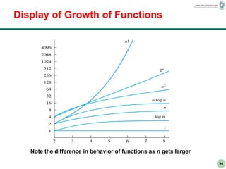
Order of growth of some common functions
O(1) < O(log n) < O(n) < O(n * log n) < O(n2
) < O(n3
) < O(2n
)
54. 54
Display of Growth of Functions
Note the difference in behavior of functions as n gets larger
56. 56
The Growth of Combinations of
Functions
If f1 (x) is O(g1(x)) and f2 (x) is O(g2(x)) then
( f1 + f2 )(x) is O(max(|g1(x) |,|g2(x) |)).
Example: what is order of 2n+log n
2n+log n is O(n)
If f1 (x) is O(g1(x)) and f2 (x) is O(g2(x)) then
( f1 f2 )(x) is O(g1(x)g2(x)).
Example: what is order of (3n+1)*(2n+log n)?
(
3n+1
(*)
2n+log n
)
is O(n*n)=O(n2
)
57. 57
Complexity Analysis : Loops
The running time of a loop is, at most, the running time of the
statements inside the loop (including tests) multiplied by the number
of iterations.
for (i=1; i<=n; i++)
{
s = s + 2;
}
constant time
executed
n times
Total time = a constant c * n = cn = O(N)
58. 58
Complexity Analysis : Nested loops
Analyse inside out. Total running time is the product of the
sizes of all the loops.
for (i=1; i<=n; i++) {
for (j=1; j<=n; j++) {
s = s+1;
}
}
constant time
outer loop
executed
n times
inner loop
executed
n times
Total time = c * n * n * = cn2
= O(N2
)
59. 59
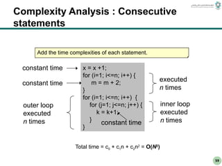
Complexity Analysis : Consecutive
statements
Add the time complexities of each statement.
x = x +1;
for (i=1; i<=n; i++) {
m = m + 2;
}
for (i=1; i<=n; i++) {
for (j=1; j<=n; j++) {
k = k+1;
}
}
inner loop
executed
n times
outer loop
executed
n times constant time
executed
n times
constant time
constant time
Total time = c0 + c1n + c2n2
= O(N2
)
60. 60
Complexity Analysis : If-then-else
statements
Worst-case running time: the test, plus either the then part or
the else part (whichever is the larger).
if ( n<0) {
return 0;
}
else
{
for (int i = 0; i < n. i++) {
s=s+i;
}
return S;
}
then part:
constant
else part:
(constant +
constant) * n
test:
constant
another if :
constant +
constant
(no else part)
Total time = c0 + c1 + (c2 + c3) * n
c0
Editor's Notes
#53: Show that the order of function is strict.
Another example: which one is bigger n^1.001 or n*log n?


![30
Example of Basic Operations:
Arithmetic operations
- ,+ ,% ,/ ,* :
x = 5 * y - z
;
Boolean operations
! ,|| ,&& :
(
x < 12
)
&&
(
y > 1
)
Assignment statements of simple data types
int x = y
;
Simple conditional tests
:
if (x < 12)
...
Memory Access (includes array indexing)
:
A[j] = 5
;
Method calls (The execution time of a method itself may not be constant)
:
System.out.printn(j)
A method's return statement
:
Return sum
We consider an operation such as ++ , += , and *= as consisting of two basic
operations : i
++](https://image.slidesharecdn.com/chap3algorithm1-250227153009-574c25a2/85/CHAP-3-ALGORITHM-for-infomatique-ingenieure-ppt-30-320.jpg)
![31
Complexity Analysis :Example
// Input: int A[N], array of N integers
// Output: Sum of all numbers in array A
int Sum(int A[], int N {
int s=0;
for (int i=0; i< N; i++) {
s = s + A[i];
}
return s;
}
1
2 3 4
5
6 7
8
1,2,8: Once
3,4,5,6,7: Once per each iteration
of for loop (only 4: 2 Once),
N iteration
Total: 6N + 3
The complexity function of the
algorithm is : f(N) = 6N +4 (n+1
loop condition )
Find the exact number of basic operations in the following
program fragment:](https://image.slidesharecdn.com/chap3algorithm1-250227153009-574c25a2/85/CHAP-3-ALGORITHM-for-infomatique-ingenieure-ppt-31-320.jpg)