


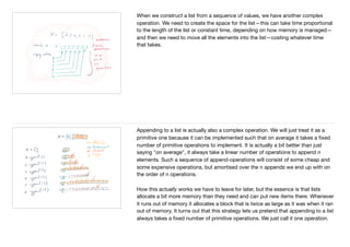
![If you delete an element inside the list, you need to copy all the preceding items,
so that is also an operation that requires a number of primitive operations that is
proportional to the number of items copied. (You can delete the last element with a
few operations because you do not need to copy any items in that case).
Assumptions:
• All primitive operations take the
same time
• The cost of complex operations
is the sum of their primitive
operations
When we figure out how much time it takes to solve a particular problem, we
simply count the number of primitive operations the task takes. We do not
distinguish between the types of operations—that would be too hard, trust me, and
wouldn’t necessarily map well to actual hardware.
In all honesty, I am lying when I tell you that there even are such things as complex
operations. There are operations in Python that looks like they are operations at the
same level as getting the value at index i in list x, x[i], but are actually more
complicated. I call such things "complex operations", but the only reason that I
have to distinguish between primitive and complex operations is that a lot is
hidden from you when you ask Python to do such things as concatenate two lists
(or two strings) or when you slice out parts of a list. At the most primitive level, the
computer doesn’t have complex operations. If you had to implement Python based
only one the primitive operations you have there, then you would appreciate that](https://image.slidesharecdn.com/chapter4-algorithmicefficiencyhandoutswithnotes-181112062536/85/Chapter-4-algorithmic-efficiency-handouts-with-notes-5-320.jpg)
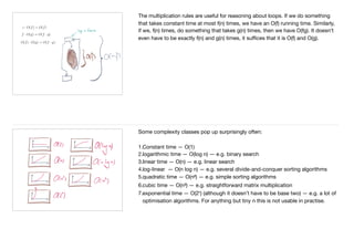
![For some operations it isn’t necessarily clear exactly how many primitive
operations we need.
Can we assign to and read from variables in constant time? If we equate variable
names with memory locations, then yes, but otherwise it might be more complex.
When we do an operation such as "x = x + 5" do we count that as "read the value
of x" then "add 5 to it" and finally "put the result in the memory location referred to
as x"? That would be three operations. But hardware might support adding a
constant to a location as a single operation—quite frequently—so "x += 5" might
be faster; only one primitive operation.
Similarly, the number of operations it takes to access or update items at a given
index into a list can vary depending on how we imagine they are done. If the
variable x indicates the start address of the elements in the list (ignoring where we
store the length of the list), then we can get index i by adding i to x: x[0] is memory
address x, x[1] is memory address x + 1, …, x[i] is memory address x + i. Getting
that value could be
1.get x
2.add i
3.read has is at the address x+i
that would be three operations. Most hardware can combine some of them,
though. There are instructions that can take a location and an offset and get the
value in that word as a single instruction. That would be](https://image.slidesharecdn.com/chapter4-algorithmicefficiencyhandoutswithnotes-181112062536/85/Chapter-4-algorithmic-efficiency-handouts-with-notes-6-320.jpg)


More Related Content
What's hot (20)
Similar to Chapter 4 algorithmic efficiency handouts (with notes) (20)


More from mailund (20)


Recently uploaded (20)


Chapter 4 algorithmic efficiency handouts (with notes)
- 1. Chapter 4 Algorithmic Complexity/Efficiency To think about the complexity of computation, we need a model of reality. As with everything else in the real world, we cannot handle the full complexity, so we make some simplifications that enables us to reason about the world.
- 2. A common model in computer science is the RAM (random access memory) model. It is the model that we will use. It shares some commonalities with other models, though not all, so do not think that the explanation here is unique to the RAM model, but different models can have slightly different assumptions about what you can do as "primitive" operations and which you cannot. That is usually the main difference between them; another is the cost of operations that can vary from model to model. Common for most the models is an assumption about what you can do with numbers, especially what you can do with numbers smaller than the input size. The space it takes to store a number, and the time it takes to operate on it, is not constant. The number of bits you need to store and manipulate depends on the size of the number. Many list operations will also be primitive in the RAM model. Not because the RAM model knows anything about Python lists—it doesn’t—but because we can express Python lists in terms of the RAM model (with some assumptions about how lists are represented). The RAM has a concept of memory as contiguous "memory words", and a Python list can thought of as a contiguous sequence of memory words. (Things get a little bit more complex if lists store something other than numbers, but we don’t care about that right now). Lists also explicitly store their length, so we can get that without having to run through the list and count. In the RAM model we can get what is at any memory location as a primitive operation and we can store a value at any memory location as a primitive operation. To get the index of a list, we get the memory location of the list and then
- 3. If we have this idea of lists as contiguous memory locations, we can see that concatenation of lists is not a single primitive operation. To make the list x + y, we need to create a new list to store the concatenated list and then we need to copy all the elements from both x and y into it. So, with lists, we can get their length and values at any index one or a few operations. It is less obvious, but we can also append to lists in a few (constant number) primitive operations—I’ll sketch how shortly, but otherwise just trust me on this. Concatenating two lists, or extending one with another, are not primitive operations; neither is deleting an element in the middle of a list.
- 4. You can see that the primitive list operations map to one or perhaps a handful of primitive operations in a model that just work with memory words, simply by mapping a list to a sequence of words. The append operation is—as I said—a bit more complex, but it works because we have usually allocated a bit more memory than we need for a list, so we have empty words following the list items, and we can put the appended value there. This doesn’t always work, because sometimes we run out of this extra memory, and then we need to do more. We can set it up such that this happens sufficiently infrequently that appending takes a few primitive operations on average. Thinking of the lists as contiguous blocks of memory also makes it clear why concatenating and extending lists are not primitive, but requires a number of operations proportional to the lengths of the lists.
- 5. If you delete an element inside the list, you need to copy all the preceding items, so that is also an operation that requires a number of primitive operations that is proportional to the number of items copied. (You can delete the last element with a few operations because you do not need to copy any items in that case). Assumptions: • All primitive operations take the same time • The cost of complex operations is the sum of their primitive operations When we figure out how much time it takes to solve a particular problem, we simply count the number of primitive operations the task takes. We do not distinguish between the types of operations—that would be too hard, trust me, and wouldn’t necessarily map well to actual hardware. In all honesty, I am lying when I tell you that there even are such things as complex operations. There are operations in Python that looks like they are operations at the same level as getting the value at index i in list x, x[i], but are actually more complicated. I call such things "complex operations", but the only reason that I have to distinguish between primitive and complex operations is that a lot is hidden from you when you ask Python to do such things as concatenate two lists (or two strings) or when you slice out parts of a list. At the most primitive level, the computer doesn’t have complex operations. If you had to implement Python based only one the primitive operations you have there, then you would appreciate that
- 6. For some operations it isn’t necessarily clear exactly how many primitive operations we need. Can we assign to and read from variables in constant time? If we equate variable names with memory locations, then yes, but otherwise it might be more complex. When we do an operation such as "x = x + 5" do we count that as "read the value of x" then "add 5 to it" and finally "put the result in the memory location referred to as x"? That would be three operations. But hardware might support adding a constant to a location as a single operation—quite frequently—so "x += 5" might be faster; only one primitive operation. Similarly, the number of operations it takes to access or update items at a given index into a list can vary depending on how we imagine they are done. If the variable x indicates the start address of the elements in the list (ignoring where we store the length of the list), then we can get index i by adding i to x: x[0] is memory address x, x[1] is memory address x + 1, …, x[i] is memory address x + i. Getting that value could be 1.get x 2.add i 3.read has is at the address x+i that would be three operations. Most hardware can combine some of them, though. There are instructions that can take a location and an offset and get the value in that word as a single instruction. That would be
- 7. When we have operations that involve moving or looking at more than one memory word we have a complex operation. These operations typically take time proportional to how many elements you look at your or you move around. Extending a list is also a complex operation. We do not (necessarily) need to copy the vector we modify, but we do need to copy all the elements from the second vector.
- 8. When we construct a list from a sequence of values, we have another complex operation. We need to create the space for the list—this can take time proportional to the length of the list or constant time, depending on how memory is managed— and then we need to move all the elements into the list—costing whatever time that takes. Appending to a list is actually also a complex operation. We will just treat it as a primitive one because it can be implemented such that on average it takes a fixed number of primitive operations to implement. It is actually a bit better than just saying "on average", it always take a linear number of operations to append n elements. Such a sequence of append-operations will consist of some cheap and some expensive operations, but amortised over the n appends we end up with on the order of n operations. How this actually works we have to leave for later, but the essence is that lists allocate a bit more memory than they need and can put new items there. Whenever it runs out of memory it allocates a block that is twice as large as it was when it ran out of memory. It turns out that this strategy lets us pretend that appending to a list always takes a fixed number of primitive operations. We just call it one operation.
- 9. When we discuss the complexity of an algorithm, we usually discard the cost of getting the input of passing on the output. We assume that the input is given to us in a form that we can immediately use, and we assume that the way we leave the output matches what the next computation needs. We usually measure the cost of running an algorithm as a function of the input size. This, by convention, we call n. It is usually not a problem to see what the size of the input is. If you get a list, it is the length of the list. If it is a string, it is the length of the string. If it is a graph—like the connected component algorithm from the previous chapter—then it is the number of nodes and the number of edges (cities and roads in that example). One case where it might be a bit strange is when numbers are involved. It takes log n bits (log base 2) to represent the number n. So if we have a list of n numbers, all smaller than n, is the input size then n × log n? Of if the input is just a number do we have n=1 or the log of that number? This is an issue, but it hardly ever matters. Unless you use numbers larger than
- 10. To work out the complexity of an algorithm (or, with a positive spin on it, the efficiency) we count how many operations it takes on input of size n. Best case? Average case? Worst case? Sometimes, the running time is not just a function of the size of the input but also what the actual input is. Taking into account all possible input to give a measure of algorithmic efficiency is impractical, so we use instead consider best, average and worst-case running times.
- 11. = n Counting the actual number of operations is tedious and pointless—it doesn’t directly translate into running time anyway. We therefore only care about the "order" of the complexity. The "Big-Oh of f" class of functions, for some specific function f, are those that f can dominate after a while if we get to multiply it with a constant. If g is in O(f) it doesn’t mean that g(n) is smaller than f(n). It is possible that g(n) is always larger than f(n). But it does mean that we can multiply f with a constant c such that cf(n) >= g(n) (eventually). The "eventually" means that after some n it is always the case. It doesn’t mean that cf(n) is always larger than g(n). For some finite number of points at the beginning of the n axis it can be larger.
- 12. You get big-Omega by changing which function should dominate which. If g is in O(f) then f is in Ω(g). (If both, then g is in Θ(f) and f is in Θ(g)). If you do the arithmetic (for function addition, i.e. (f₁ + f₂)(x) = f₁(x) + f₂(x) and (f · g) (x) = f(x) × g(x)) it is not hard to show these properties. The second and third are just special cases of the first, but we use these two more often than the others. The second rule tells us that if we have different phases in an algorithm, then we can add the complexity of those to get the complexity of the algorithm. The third rule tells us that we really only care about the slowest step of an algorithm — it dominates all the other steps.
- 13. The multiplication rules are useful for reasoning about loops. If we do something that takes constant time at most f(n) times, we have an O(f) running time. Similarly, if we, f(n) times, do something that takes g(n) times, then we have O(fg). It doesn’t even have to be exactly f(n) and g(n) times, it suffices that it is O(f) and O(g). Some complexity classes pop up surprisingly often: 1.Constant time — O(1) 2.logarithmic time — O(log n) — e.g. binary search 3.linear time — O(n) — e.g. linear search 4.log-linear — O(n log n) — e.g. several divide-and-conquer sorting algorithms 5.quadratic time — O(n²) — e.g. simple sorting algorithms 6.cubic time — O(n³) — e.g. straightforward matrix multiplication 7.exponential time — O(2ⁿ) (although it doesn’t have to be base two) — e.g. a lot of optimisation algorithms. For anything but tiny n this is not usable in practise.
- 14. Thats it! Now it is time to do the exercises to test that you now understand algorithmic complexity