Cleaned_Lecture 6666666_Simulation_I.pdf

Lecture 6:
Simulation
Professor
Amany E. Aly
Simulation
Monte Carlo
simulation
Generation of
pseudorandom
numbers
Simulation of
other random
variables
Bernoulli
random
variables
Binomial
random
variables
Poisson random
variables
Exponential
random
numbers
Normal random
variables
Generating
normal variates
using the
Box-Müller
transformation
Lecture 6: Simulation
Professor Amany E. Aly
Department of Mathematics, Faculty of Science,
Helwan University, Ain Helwan, Cairo, Egypt.
18 / 11 / 2024
Professor Amany E. Aly ( Department of Mathematics, Faculty of Science, Helwan University, Ain Helwan, Cairo, Egypt.)
Lecture 6: Simulation 18 / 11 / 2024 1 / 99

Lecture 6:
Simulation
Professor
Amany E. Aly
Simulation
Monte Carlo
simulation
Generation of
pseudorandom
numbers
Simulation of
other random
variables
Bernoulli
random
variables
Binomial
random
variables
Poisson random
variables
Exponential
random
numbers
Normal random
variables
Generating
normal variates
using the
Box-Müller
transformation
Presentation Outline
1 Simulation
Monte Carlo simulation
Generation of pseudorandom numbers
Simulation of other random variables
Bernoulli random variables
Binomial random variables
Poisson random variables
Exponential random numbers
Normal random variables
Generating normal variates using the Box-Müller transformation
All built-in distributions

Lecture 6:
Simulation
Professor
Amany E. Aly
Simulation
Monte Carlo
simulation
Generation of
pseudorandom
numbers
Simulation of
other random
variables
Bernoulli
random
variables
Binomial
random
variables
Poisson random
variables
Exponential
random
numbers
Normal random
variables
Generating
normal variates
using the
Box-Müller
transformation
Much of statistics relies on being able to
evaluate expectations of random variables,
finding quantiles of distributions.
For example:

Lecture 6:
Simulation
Professor
Amany E. Aly
Simulation
Monte Carlo
simulation
Generation of
pseudorandom
numbers
Simulation of
other random
variables
Bernoulli
random
variables
Binomial
random
variables
Poisson random
variables
Exponential
random
numbers
Normal random
variables
Generating
normal variates
using the
Box-Müller
transformation
In hypothesis testing, the p-value of a sample is defined as
the probability of observing data at least as extreme as the
sample in hand, given that the null hypothesis is true. This is
the expected value of a random variable defined to be 0 when
a sample is less extreme, and 1 otherwise.
The bias of an estimator is defined to be the expected value
of the estimator minus the true value that it is estimating.
Confidence intervals are based on quantiles of the distribution
of a pivotal quantity, e.g.(X − µ)/(s/
√
n) .

Lecture 6:
Simulation
Professor
Amany E. Aly
Simulation
Monte Carlo
simulation
Generation of
pseudorandom
numbers
Simulation of
other random
variables
Bernoulli
random
variables
Binomial
random
variables
Poisson random
variables
Exponential
random
numbers
Normal random
variables
Generating
normal variates
using the
Box-Müller
transformation
Chapter objectives
You will be introduced to Monte Carlo simulation. This intro-
duction will include basic ideas of random (or more properly,
pseudorandom) number generation.
You will then see how to simulate random variables from sev-
eral of the common probability distributions.
Next, we will show you how simulation can be used
to model natural processes,
to evaluate integrals.
The final topics is Markov chains, as well as rejection and
importance sampling will give you a hint as to what more
advanced methods are like.

Lecture 6:
Simulation
Professor
Amany E. Aly
Simulation
Monte Carlo
simulation
Generation of
pseudorandom
numbers
Simulation of
other random
variables
Bernoulli
random
variables
Binomial
random
variables
Poisson random
variables
Exponential
random
numbers
Normal random
variables
Generating
normal variates
using the
Box-Müller
transformation
Monte Carlo simulation
One of the most general computer-based methods for approximat-
ing properties of random variables is the Monte Carlo method.

Lecture 6:
Simulation
Professor
Amany E. Aly
Simulation
Monte Carlo
simulation
Generation of
pseudorandom
numbers
Simulation of
other random
variables
Bernoulli
random
variables
Binomial
random
variables
Poisson random
variables
Exponential
random
numbers
Normal random
variables
Generating
normal variates
using the
Box-Müller
transformation
To approximate the mean µ = E(X) using the Monte Carlo
method,
Generate m independent and identically distributed (i.i.d.)
copies of X, namely X1, ..., Xm,
Use the sample mean X = (1/m)
P
Xi as an estimate of
E(X).
For large values of m, X gives a good approximation to E(X).

Lecture 6:
Simulation
Professor
Amany E. Aly
Simulation
Monte Carlo
simulation
Generation of
pseudorandom
numbers
Simulation of
other random
variables
Bernoulli
random
variables
Binomial
random
variables
Poisson random
variables
Exponential
random
numbers
Normal random
variables
Generating
normal variates
using the
Box-Müller
transformation
Furthermore, if m is large the distribution of the sample mean,
X , can be approximated by a normal distribution with mean
µ and variance σ2
/m ( using central limit theorem ).
Here σ2
is the variance V ar(X), which can be approximated
by the sample variance s2
= [1/(m − 1)]
P
(Xi − X
2
).
This allows us to construct approximate confidence intervals
for µ. For example, X ± 1.96s/
√
m will contain µ approxi-
mately 95% of the time.

Lecture 6:
Simulation
Professor
Amany E. Aly
Simulation
Monte Carlo
simulation
Generation of
pseudorandom
numbers
Simulation of
other random
variables
Bernoulli
random
variables
Binomial
random
variables
Poisson random
variables
Exponential
random
numbers
Normal random
variables
Generating
normal variates
using the
Box-Müller
transformation
Generation of pseudorandom numbers
We will describe one of the simplest methods for simulating
independent uniform random variables on the interval [0,1].
A multiplicative congruential random number generator pro-
duces a sequence of pseudorandom numbers, u0, u1, u2, ...,
which appear similar to independent uniform random variables
on the interval [0,1].

Lecture 6:
Simulation
Professor
Amany E. Aly
Simulation
Monte Carlo
simulation
Generation of
pseudorandom
numbers
Simulation of
other random
variables
Bernoulli
random
variables
Binomial
random
variables
Poisson random
variables
Exponential
random
numbers
Normal random
variables
Generating
normal variates
using the
Box-Müller
transformation
Let m be a large integer, and let b be another integer which
is smaller than m.
The value of b is often chosen to be near the square root of
m.
Different values of b and m give rise to pseudorandom number
generators of varying quality.
There are various criteria available for choosing good values
of these parameters, but it is always important to test the
resulting generator to ensure that it is providing reasonable
results.

Lecture 6:
Simulation
Professor
Amany E. Aly
Simulation
Monte Carlo
simulation
Generation of
pseudorandom
numbers
Simulation of
other random
variables
Bernoulli
random
variables
Binomial
random
variables
Poisson random
variables
Exponential
random
numbers
Normal random
variables
Generating
normal variates
using the
Box-Müller
transformation
To begin, an integer x0 is chosen between 1 and m. x0 is
called the seed.
We discuss strategies for choosing x0 below.
Once the seed has been chosen, the generator proceeds as
follows:
x1 = b x0 (mod m),
u1 = x1/m.
u1 is the first pseudorandom number, taking some value be-
tween 0 and 1.

Lecture 6:
Simulation
Professor
Amany E. Aly
Simulation
Monte Carlo
simulation
Generation of
pseudorandom
numbers
Simulation of
other random
variables
Bernoulli
random
variables
Binomial
random
variables
Poisson random
variables
Exponential
random
numbers
Normal random
variables
Generating
normal variates
using the
Box-Müller
transformation
The second pseudorandom number is then obtained in the
same manner:
x2 = b x1(mod m),
u2 = x2/m.
u2 is another pseudorandom number.
If m and b are chosen properly and are not disclosed to the
user, it is difficult to predict the value of u2, given the value
of u1 only.

Lecture 6:
Simulation
Professor
Amany E. Aly
Simulation
Monte Carlo
simulation
Generation of
pseudorandom
numbers
Simulation of
other random
variables
Bernoulli
random
variables
Binomial
random
variables
Poisson random
variables
Exponential
random
numbers
Normal random
variables
Generating
normal variates
using the
Box-Müller
transformation
In other words, for most practical purposes u2 is approximately
independent of u1.
The method continues according to the following formulas:
xn = b xn−1 (mod m),
un = xn/m.
This method produces numbers which are entirely determinis-
tic, but to an observer who doesn’t know the formula above,
the numbers appear to be random and unpredictable, at least
in the short term.

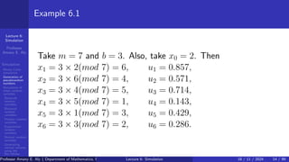
Lecture 6:
Simulation
Professor
Amany E. Aly
Simulation
Monte Carlo
simulation
Generation of
pseudorandom
numbers
Simulation of
other random
variables
Bernoulli
random
variables
Binomial
random
variables
Poisson random
variables
Exponential
random
numbers
Normal random
variables
Generating
normal variates
using the
Box-Müller
transformation
Example 6.1
Take m = 7 and b = 3. Also, take x0 = 2. Then
x1 = 3 × 2(mod 7) = 6, u1 = 0.857,
x2 = 3 × 6(mod 7) = 4, u2 = 0.571,
x3 = 3 × 4(mod 7) = 5, u3 = 0.714,
x4 = 3 × 5(mod 7) = 1, u4 = 0.143,
x5 = 3 × 1(mod 7) = 3, u5 = 0.429,
x6 = 3 × 3(mod 7) = 2, u6 = 0.286.

Lecture 6:
Simulation
Professor
Amany E. Aly
Simulation
Monte Carlo
simulation
Generation of
pseudorandom
numbers
Simulation of
other random
variables
Bernoulli
random
variables
Binomial
random
variables
Poisson random
variables
Exponential
random
numbers
Normal random
variables
Generating
normal variates
using the
Box-Müller
transformation
It should be clear that the iteration will set x7 = x1 and cycle
xi through the same sequence of integers, so the corresponding
sequence ui will also be cyclic.
An observer might not easily be able to predict u2 from u1,
but since ui+6 = ui for all i > 0, longer sequences are very
easy to predict.

Lecture 6:
Simulation
Professor
Amany E. Aly
Simulation
Monte Carlo
simulation
Generation of
pseudorandom
numbers
Simulation of
other random
variables
Bernoulli
random
variables
Binomial
random
variables
Poisson random
variables
Exponential
random
numbers
Normal random
variables
Generating
normal variates
using the
Box-Müller
transformation
In order to produce an unpredictable sequence, it is desirable
to have a very large cycle length so that it is unlikely that any
observer will ever see a whole cycle.
The cycle length cannot be any larger than m, so m would
normally be taken to be very large.

Lecture 6:
Simulation
Professor
Amany E. Aly
Simulation
Monte Carlo
simulation
Generation of
pseudorandom
numbers
Simulation of
other random
variables
Bernoulli
random
variables
Binomial
random
variables
Poisson random
variables
Exponential
random
numbers
Normal random
variables
Generating
normal variates
using the
Box-Müller
transformation
Care must be taken in the choice of b and m to ensure that
the cycle length is actually m.
Note, for example, what happens when b = 171 and m =
29241. Start with x0 = 3, say.
x1 = 171 × 3 = 513,
x2 = 171 × 513 (mod 29241) = 0.
All remaining xn values will be 0.
To avoid this kind of problem, we should choose m so that it
is not divisible by b; thus, prime values of m will be preferred.

Lecture 6:
Simulation
Professor
Amany E. Aly
Simulation
Monte Carlo
simulation
Generation of
pseudorandom
numbers
Simulation of
other random
variables
Bernoulli
random
variables
Binomial
random
variables
Poisson random
variables
Exponential
random
numbers
Normal random
variables
Generating
normal variates
using the
Box-Müller
transformation
Example 6.2
The following lines produce 50 pseudorandom numbers based on
the multiplicative congruential generator:
xn = 171xn−1 (mod 30269),
un = xn/30269,
with initial seed x0 = 27218.

Lecture 6:
Simulation
Professor
Amany E. Aly
Simulation
Monte Carlo
simulation
Generation of
pseudorandom
numbers
Simulation of
other random
variables
Bernoulli
random
variables
Binomial
random
variables
Poisson random
variables
Exponential
random
numbers
Normal random
variables
Generating
normal variates
using the
Box-Müller
transformation
The results, stored in the vector random.number, are as follows.

Lecture 6:
Simulation
Professor
Amany E. Aly
Simulation
Monte Carlo
simulation
Generation of
pseudorandom
numbers
Simulation of
other random
variables
Bernoulli
random
variables
Binomial
random
variables
Poisson random
variables
Exponential
random
numbers
Normal random
variables
Generating
normal variates
using the
Box-Müller
transformation

Lecture 6:
Simulation
Professor
Amany E. Aly
Simulation
Monte Carlo
simulation
Generation of
pseudorandom
numbers
Simulation of
other random
variables
Bernoulli
random
variables
Binomial
random
variables
Poisson random
variables
Exponential
random
numbers
Normal random
variables
Generating
normal variates
using the
Box-Müller
transformation
Note that the vector elements range between 0 and 1. These are
the pseudorandom numbers, u1, u2, ..., u50.

Lecture 6:
Simulation
Professor
Amany E. Aly
Simulation
Monte Carlo
simulation
Generation of
pseudorandom
numbers
Simulation of
other random
variables
Bernoulli
random
variables
Binomial
random
variables
Poisson random
variables
Exponential
random
numbers
Normal random
variables
Generating
normal variates
using the
Box-Müller
transformation
A similar kind of operation (though using a different formula,
and with a much longer cycle) is used internally by R to pro-
duce pseudorandom numbers automatically with the function
runif().
Syntax
runif(n, min = a, max = b)
Execution of this command produces n pseudorandom uniform
numbers on the interval [a, b].
The default values are a = 0 and b = 1.
The seed is selected internally.

Lecture 6:
Simulation
Professor
Amany E. Aly
Simulation
Monte Carlo
simulation
Generation of
pseudorandom
numbers
Simulation of
other random
variables
Bernoulli
random
variables
Binomial
random
variables
Poisson random
variables
Exponential
random
numbers
Normal random
variables
Generating
normal variates
using the
Box-Müller
transformation
Example 6.3
Generate 5 uniform pseudorandom numbers on the interval
[0, 1],
Generate 10 uniform such numbers on the interval [−3, −1].

Lecture 6:
Simulation
Professor
Amany E. Aly
Simulation
Monte Carlo
simulation
Generation of
pseudorandom
numbers
Simulation of
other random
variables
Bernoulli
random
variables
Binomial
random
variables
Poisson random
variables
Exponential
random
numbers
Normal random
variables
Generating
normal variates
using the
Box-Müller
transformation
If you execute the above code yourself, you will almost certain-
ly obtain different results than those displayed in our output.
This is because the starting seed that you will use will be
different from the one that was selected when we ran our
code.

Lecture 6:
Simulation
Professor
Amany E. Aly
Simulation
Monte Carlo
simulation
Generation of
pseudorandom
numbers
Simulation of
other random
variables
Bernoulli
random
variables
Binomial
random
variables
Poisson random
variables
Exponential
random
numbers
Normal random
variables
Generating
normal variates
using the
Box-Müller
transformation
Strategies for choosing the starting seed x0
There are two different strategies for choosing the starting seed
x0.

Lecture 6:
Simulation
Professor
Amany E. Aly
Simulation
Monte Carlo
simulation
Generation of
pseudorandom
numbers
Simulation of
other random
variables
Bernoulli
random
variables
Binomial
random
variables
Poisson random
variables
Exponential
random
numbers
Normal random
variables
Generating
normal variates
using the
Box-Müller
transformation
The first strategy for choosing x0
If the goal is to make an unpredictable sequence, then a ran-
dom value is desirable.
For example, the computer might determine the current time
of day to the nearest millisecond, then base the starting seed
on the number of milliseconds past the start of the minute.
To avoid predictability, this external randomization should only
be done once, after which the formula above should be used
for updates.

Lecture 6:
Simulation
Professor
Amany E. Aly
Simulation
Monte Carlo
simulation
Generation of
pseudorandom
numbers
Simulation of
other random
variables
Bernoulli
random
variables
Binomial
random
variables
Poisson random
variables
Exponential
random
numbers
Normal random
variables
Generating
normal variates
using the
Box-Müller
transformation
For example, if the computer clock were used as above before gen-
erating every ui, on a fast computer there would be long sequences
of identical values that were generated within a millisecond of each
other.

Lecture 6:
Simulation
Professor
Amany E. Aly
Simulation
Monte Carlo
simulation
Generation of
pseudorandom
numbers
Simulation of
other random
variables
Bernoulli
random
variables
Binomial
random
variables
Poisson random
variables
Exponential
random
numbers
Normal random
variables
Generating
normal variates
using the
Box-Müller
transformation
The second strategy for choosing x0
The second strategy for choosing x0 is to use a fixed, non-random
value, e.g. x0 = 1.
This makes the sequence of ui values predictable and repeat-
able.
This would be useful when debugging a program that uses
random numbers, or in other situations where repeatability is
needed.
The way to do this in R is to use the set.seed() function.

Lecture 6:
Simulation
Professor
Amany E. Aly
Simulation
Monte Carlo
simulation
Generation of
pseudorandom
numbers
Simulation of
other random
variables
Bernoulli
random
variables
Binomial
random
variables
Poisson random
variables
Exponential
random
numbers
Normal random
variables
Generating
normal variates
using the
Box-Müller
transformation
For example,

Lecture 6:
Simulation
Professor
Amany E. Aly
Simulation
Monte Carlo
simulation
Generation of
pseudorandom
numbers
Simulation of
other random
variables
Bernoulli
random
variables
Binomial
random
variables
Poisson random
variables
Exponential
random
numbers
Normal random
variables
Generating
normal variates
using the
Box-Müller
transformation
Solve exercises from 1 to 10 on pages 154, 155, and 156 .

Lecture 6:
Simulation
Professor
Amany E. Aly
Simulation
Monte Carlo
simulation
Generation of
pseudorandom
numbers
Simulation of
other random
variables
Bernoulli
random
variables
Binomial
random
variables
Poisson random
variables
Exponential
random
numbers
Normal random
variables
Generating
normal variates
using the
Box-Müller
transformation
Bernoulli random variables
A Bernoulli trial is an experiment in which there are only two
possible outcomes. For example, a light bulb may work or not
work; these are the only possibilities.
Each outcome (”work” or ”not work”) has a probability as-
sociated with it; the sum of these two probabilities must be
1.

Lecture 6:
Simulation
Professor
Amany E. Aly
Simulation
Monte Carlo
simulation
Generation of
pseudorandom
numbers
Simulation of
other random
variables
Bernoulli
random
variables
Binomial
random
variables
Poisson random
variables
Exponential
random
numbers
Normal random
variables
Generating
normal variates
using the
Box-Müller
transformation
Example 6.4
Consider a student who guesses on a multiple choice test ques-
tion which has five options; the student may guess correctly with
probability 0.2 and incorrectly with probability 0.8. (The possible
outcome of a guess is to either be correct or to be incorrect.)
Suppose we would like to know how well such a student would do
on a multiple choice test consisting of 20 questions. We can get
an idea by using simulation.

Lecture 6:
Simulation
Professor
Amany E. Aly
Simulation
Monte Carlo
simulation
Generation of
pseudorandom
numbers
Simulation of
other random
variables
Bernoulli
random
variables
Binomial
random
variables
Poisson random
variables
Exponential
random
numbers
Normal random
variables
Generating
normal variates
using the
Box-Müller
transformation
Each question corresponds to an independent Bernoulli trial
with probability of success equal to 0.2.
We can simulate the correctness of the student for each ques-
tion by generating an independent uniform random number.
If this number is less than 0.2, we say that the student guessed
correctly; otherwise, we say that the student guessed incorrect-
ly.

Lecture 6:
Simulation
Professor
Amany E. Aly
Simulation
Monte Carlo
simulation
Generation of
pseudorandom
numbers
Simulation of
other random
variables
Bernoulli
random
variables
Binomial
random
variables
Poisson random
variables
Exponential
random
numbers
Normal random
variables
Generating
normal variates
using the
Box-Müller
transformation
This will work, because the probability that a uniform random
variable is less than 0.2 is exactly 0.2, while the probability
that a uniform random variable exceeds 0.2 is exactly 0.8,
which is the same as the probability that the student guesses
incorrectly.
Thus, the uniform random number generator is simulating the
student.

Lecture 6:
Simulation
Professor
Amany E. Aly
Simulation
Monte Carlo
simulation
Generation of
pseudorandom
numbers
Simulation of
other random
variables
Bernoulli
random
variables
Binomial
random
variables
Poisson random
variables
Exponential
random
numbers
Normal random
variables
Generating
normal variates
using the
Box-Müller
transformation
R can do this as follows:

Lecture 6:
Simulation
Professor
Amany E. Aly
Simulation
Monte Carlo
simulation
Generation of
pseudorandom
numbers
Simulation of
other random
variables
Bernoulli
random
variables
Binomial
random
variables
Poisson random
variables
Exponential
random
numbers
Normal random
variables
Generating
normal variates
using the
Box-Müller
transformation
The vector correct.answers is a logical vector which contains
the results of the simulated student’s guesses;
A TRUE value corresponds to a correct guess, while a FALSE
corresponds to an incorrect guess.
The total number of correct guesses can be calculated.
Our simulated student would score 6/20.

Lecture 6:
Simulation
Professor
Amany E. Aly
Simulation
Monte Carlo
simulation
Generation of
pseudorandom
numbers
Simulation of
other random
variables
Bernoulli
random
variables
Binomial
random
variables
Poisson random
variables
Exponential
random
numbers
Normal random
variables
Generating
normal variates
using the
Box-Müller
transformation
In the preceding example, we could associate the values ”1”
and ”0” with the outcomes from a Bernoulli trial.
This defines the Bernoulli random variable: a random vari-
able which takes the value 1 with probability p, and 0 with
probability 1 − p.
The expected value of a Bernoulli random variable is p and its
theoretical variance is p(1 − p).
In the above example, a student would expect to guess cor-
rectly 20% of the time; our simulated student was a little bit
lucky, obtaining a mark of 30%.

Lecture 6:
Simulation
Professor
Amany E. Aly
Simulation
Monte Carlo
simulation
Generation of
pseudorandom
numbers
Simulation of
other random
variables
Bernoulli
random
variables
Binomial
random
variables
Poisson random
variables
Exponential
random
numbers
Normal random
variables
Generating
normal variates
using the
Box-Müller
transformation
Solve exercises from 1 to 4 on page 157.

Lecture 6:
Simulation
Professor
Amany E. Aly
Simulation
Monte Carlo
simulation
Generation of
pseudorandom
numbers
Simulation of
other random
variables
Bernoulli
random
variables
Binomial
random
variables
Poisson random
variables
Exponential
random
numbers
Normal random
variables
Generating
normal variates
using the
Box-Müller
transformation
Binomial random variables
Let X denote the sum of m independent Bernoulli random
variables, each having probability p.
X is called a binomial random variable; it represents the num-
ber of ”successes” in m Bernoulli trials.
A binomial random variable can take values in the set 0, 1, 2, ..., m
The probability of a binomial random variable X taking on any
one of these values is governed by the binomial distribution:

Lecture 6:
Simulation
Professor
Amany E. Aly
Simulation
Monte Carlo
simulation
Generation of
pseudorandom
numbers
Simulation of
other random
variables
Bernoulli
random
variables
Binomial
random
variables
Poisson random
variables
Exponential
random
numbers
Normal random
variables
Generating
normal variates
using the
Box-Müller
transformation
P(X = x) =

m
x

px
(1 − p)m−x
, x = 0, 1, ..., m.
These probabilities can be computed using the dbinom() function.

Lecture 6:
Simulation
Professor
Amany E. Aly
Simulation
Monte Carlo
simulation
Generation of
pseudorandom
numbers
Simulation of
other random
variables
Bernoulli
random
variables
Binomial
random
variables
Poisson random
variables
Exponential
random
numbers
Normal random
variables
Generating
normal variates
using the
Box-Müller
transformation
Syntax
dbinom(x, size, prob)
Here, size and prob are the binomial parameters m and p,
respectively,
while x denotes the number of ”successes”.
The output from this function is the value of P(X = x).

Lecture 6:
Simulation
Professor
Amany E. Aly
Simulation
Monte Carlo
simulation
Generation of
pseudorandom
numbers
Simulation of
other random
variables
Bernoulli
random
variables
Binomial
random
variables
Poisson random
variables
Exponential
random
numbers
Normal random
variables
Generating
normal variates
using the
Box-Müller
transformation
Example 6.5
Compute the probability of getting four heads in six tosses of a
fair coin.
Thus, P(X = 4) = 0.234, where X is a binomial random variable
with m = 6 and p = 0.5.

Lecture 6:
Simulation
Professor
Amany E. Aly
Simulation
Monte Carlo
simulation
Generation of
pseudorandom
numbers
Simulation of
other random
variables
Bernoulli
random
variables
Binomial
random
variables
Poisson random
variables
Exponential
random
numbers
Normal random
variables
Generating
normal variates
using the
Box-Müller
transformation
Cumulative probabilities of the form P(X ⩽ x) can be com-
puted using pbinom();
This function takes the same arguments as dbinom().
For example, we can calculate P(X ⩽ 4) where X is the
number of heads obtained in six tosses of a fair coin as:

Lecture 6:
Simulation
Professor
Amany E. Aly
Simulation
Monte Carlo
simulation
Generation of
pseudorandom
numbers
Simulation of
other random
variables
Bernoulli
random
variables
Binomial
random
variables
Poisson random
variables
Exponential
random
numbers
Normal random
variables
Generating
normal variates
using the
Box-Müller
transformation
The function qbinom() gives the quantiles for the binomial
distribution.
The 89th percentile of the distribution of X (as defined above)
is:
The expected value (or mean) of a binomial random variable
is mp and the variance is mp(1 − p).

Lecture 6:
Simulation
Professor
Amany E. Aly
Simulation
Monte Carlo
simulation
Generation of
pseudorandom
numbers
Simulation of
other random
variables
Bernoulli
random
variables
Binomial
random
variables
Poisson random
variables
Exponential
random
numbers
Normal random
variables
Generating
normal variates
using the
Box-Müller
transformation
The rbinom() function can be used to generate binomial pseu-
dorandom numbers.
Syntax
rbinom(n, size, prob)
Here, size and prob are the binomial parameters, while n is
the number of variates generated.

Lecture 6:
Simulation
Professor
Amany E. Aly
Simulation
Monte Carlo
simulation
Generation of
pseudorandom
numbers
Simulation of
other random
variables
Bernoulli
random
variables
Binomial
random
variables
Poisson random
variables
Exponential
random
numbers
Normal random
variables
Generating
normal variates
using the
Box-Müller
transformation
Example 6.6
Suppose 10% of the water heater dip tubes produced by a machine
are defective, and suppose 15 tubes are produced each hour. Each
tube is independent of all other tubes. This process is judged to be
out of control when more than five defective tubes are produced in
any single hour. Simulate the number of defective tubes produced
by the machine for each hour over a 24-hour period, and determine
if any process should have been judged out of control at any point
in that simulation run.

Lecture 6:
Simulation
Professor
Amany E. Aly
Simulation
Monte Carlo
simulation
Generation of
pseudorandom
numbers
Simulation of
other random
variables
Bernoulli
random
variables
Binomial
random
variables
Poisson random
variables
Exponential
random
numbers
Normal random
variables
Generating
normal variates
using the
Box-Müller
transformation
Since 15 tubes are produced each hour and each tube has a 0.1
probability of being defective, independent of the state of the
other tubes, the number of defectives produced in one hour is
a binomial random variable with m = 15 and p = 0.1.
To simulate the number of defectives for each hour in a 24-
hour period, we need to generate 24 binomial random num-
bers.
We then identify all instances in which the number of defec-
tives exceeds 5. One such simulation run is:

Lecture 6:
Simulation
Professor
Amany E. Aly
Simulation
Monte Carlo
simulation
Generation of
pseudorandom
numbers
Simulation of
other random
variables
Bernoulli
random
variables
Binomial
random
variables
Poisson random
variables
Exponential
random
numbers
Normal random
variables
Generating
normal variates
using the
Box-Müller
transformation

Lecture 6:
Simulation
Professor
Amany E. Aly
Simulation
Monte Carlo
simulation
Generation of
pseudorandom
numbers
Simulation of
other random
variables
Bernoulli
random
variables
Binomial
random
variables
Poisson random
variables
Exponential
random
numbers
Normal random
variables
Generating
normal variates
using the
Box-Müller
transformation
Solve exercises from 1 to 7 on pages 159 to 162.

Lecture 6:
Simulation
Professor
Amany E. Aly
Simulation
Monte Carlo
simulation
Generation of
pseudorandom
numbers
Simulation of
other random
variables
Bernoulli
random
variables
Binomial
random
variables
Poisson random
variables
Exponential
random
numbers
Normal random
variables
Generating
normal variates
using the
Box-Müller
transformation
Poisson random variables
The Poisson distribution is the limit of a sequence of binomial
distributions with parameters n and pn, where n is increasing
to infinity, and pn is decreasing to 0, but where the expected
value (or mean) n pn converges to a constant λ.
The variance n pn (1 − pn) converges to this same constant.
Thus, the mean and variance of a Poisson random variable are
both equal to λ. This parameter is sometimes referred to as
a rate.

Lecture 6:
Simulation
Professor
Amany E. Aly
Simulation
Monte Carlo
simulation
Generation of
pseudorandom
numbers
Simulation of
other random
variables
Bernoulli
random
variables
Binomial
random
variables
Poisson random
variables
Exponential
random
numbers
Normal random
variables
Generating
normal variates
using the
Box-Müller
transformation
Poisson random variables arise in a number of different ways.
They are often used as a crude model for count data.
Examples of count data are the numbers of earthquakes in a
region in a given year, or the number of individuals who arrive
at a bank teller in a given hour.
The limit comes from dividing the time period into n indepen-
dent intervals, on which the count is either 0 or 1.
The Poisson random variable is the total count.

Lecture 6:
Simulation
Professor
Amany E. Aly
Simulation
Monte Carlo
simulation
Generation of
pseudorandom
numbers
Simulation of
other random
variables
Bernoulli
random
variables
Binomial
random
variables
Poisson random
variables
Exponential
random
numbers
Normal random
variables
Generating
normal variates
using the
Box-Müller
transformation
The possible values that a Poisson random variable X could
take are the nonnegative integers {0, 1, 2, ...}.
The probability of taking on any of these values is
P(X = x) =
e−x
λx
x!
, x = 0, 1, 2, ...
These probabilities can be evaluated using the dpois() func-
tion.

Lecture 6:
Simulation
Professor
Amany E. Aly
Simulation
Monte Carlo
simulation
Generation of
pseudorandom
numbers
Simulation of
other random
variables
Bernoulli
random
variables
Binomial
random
variables
Poisson random
variables
Exponential
random
numbers
Normal random
variables
Generating
normal variates
using the
Box-Müller
transformation
Syntax
dpois(x, lambda)
Here, lambda is the Poisson rate parameter, while x is the
number of Poisson events.
The output from the function is the value of P(X = x).

Lecture 6:
Simulation
Professor
Amany E. Aly
Simulation
Monte Carlo
simulation
Generation of
pseudorandom
numbers
Simulation of
other random
variables
Bernoulli
random
variables
Binomial
random
variables
Poisson random
variables
Exponential
random
numbers
Normal random
variables
Generating
normal variates
using the
Box-Müller
transformation
Example 6.7
According to the Poisson model, the probability of three arrivals
at an automatic bank teller in the next minute, where the average
number of arrivals per minute is 0.5, is
Therefore, P(X = 3) = 0.0126, if X is a Poisson random variable
with mean 0.5.

Lecture 6:
Simulation
Professor
Amany E. Aly
Simulation
Monte Carlo
simulation
Generation of
pseudorandom
numbers
Simulation of
other random
variables
Bernoulli
random
variables
Binomial
random
variables
Poisson random
variables
Exponential
random
numbers
Normal random
variables
Generating
normal variates
using the
Box-Müller
transformation
Cumulative probabilities of the form P(X ⩽ x) can be calcu-
lated using ppois(),
Poisson quantiles can be computed using qpois().

Lecture 6:
Simulation
Professor
Amany E. Aly
Simulation
Monte Carlo
simulation
Generation of
pseudorandom
numbers
Simulation of
other random
variables
Bernoulli
random
variables
Binomial
random
variables
Poisson random
variables
Exponential
random
numbers
Normal random
variables
Generating
normal variates
using the
Box-Müller
transformation
We can generate Poisson random numbers using the rpois() func-
tion.
Syntax
rpois(n, lambda)
The parameter n is the number of variates produced, and lambda
is as above.

Lecture 6:
Simulation
Professor
Amany E. Aly
Simulation
Monte Carlo
simulation
Generation of
pseudorandom
numbers
Simulation of
other random
variables
Bernoulli
random
variables
Binomial
random
variables
Poisson random
variables
Exponential
random
numbers
Normal random
variables
Generating
normal variates
using the
Box-Müller
transformation
Example 6.8
Suppose traffic accidents occur at an intersection with a mean
rate of 3.7 per year. Simulate the annual number of accidents for
a 10-year period, assuming a Poisson model.

Lecture 6:
Simulation
Professor
Amany E. Aly
Simulation
Monte Carlo
simulation
Generation of
pseudorandom
numbers
Simulation of
other random
variables
Bernoulli
random
variables
Binomial
random
variables
Poisson random
variables
Exponential
random
numbers
Normal random
variables
Generating
normal variates
using the
Box-Müller
transformation
Poisson processes
A Poisson process is a simple model of the collection of events
that occur during an interval of time.
A way of thinking about a Poisson process is to think of a
random collection of points on a line or in the plane (or in
higher dimensions, if necessary).
The homogeneous Poisson process has the following proper-
ties:
1. The distribution of the number of points in a set is Poisson with rate proportional
to the size of the set.
2. The numbers of points in non-overlapping sets are independent of each other.

Lecture 6:
Simulation
Professor
Amany E. Aly
Simulation
Monte Carlo
simulation
Generation of
pseudorandom
numbers
Simulation of
other random
variables
Bernoulli
random
variables
Binomial
random
variables
Poisson random
variables
Exponential
random
numbers
Normal random
variables
Generating
normal variates
using the
Box-Müller
transformation
In particular, for a Poisson process with rate λ the number of
points on an interval [0, T] is Poisson distributed with mean λ T.
One way to simulate this is as follows.
1. Generate N as a Poisson pseudorandom number with param-
eter λ T.
2. Generate N independent uniform pseudorandom numbers on
the interval [0, T].

Lecture 6:
Simulation
Professor
Amany E. Aly
Simulation
Monte Carlo
simulation
Generation of
pseudorandom
numbers
Simulation of
other random
variables
Bernoulli
random
variables
Binomial
random
variables
Poisson random
variables
Exponential
random
numbers
Normal random
variables
Generating
normal variates
using the
Box-Müller
transformation
Example 6.9
Simulate points of a homogeneous Poisson process having rate 1.5
on the interval [0, 10].

Lecture 6:
Simulation
Professor
Amany E. Aly
Simulation
Monte Carlo
simulation
Generation of
pseudorandom
numbers
Simulation of
other random
variables
Bernoulli
random
variables
Binomial
random
variables
Poisson random
variables
Exponential
random
numbers
Normal random
variables
Generating
normal variates
using the
Box-Müller
transformation
Solve exercises from 1 to 10 on pages 164, 165 and 166 .

Lecture 6:
Simulation
Professor
Amany E. Aly
Simulation
Monte Carlo
simulation
Generation of
pseudorandom
numbers
Simulation of
other random
variables
Bernoulli
random
variables
Binomial
random
variables
Poisson random
variables
Exponential
random
numbers
Normal random
variables
Generating
normal variates
using the
Box-Müller
transformation
Exponential random numbers
Exponential random variables are used as simple models for
such things as failure times of mechanical or electronic com-
ponents, or for the time it takes a server to complete service
to a customer.
The exponential distribution is characterized by a constant
failure rate, denoted by λ.
T has an exponential distribution with rate λ 0 if
P(T ⩽ t) = 1 − e−λ t
for any nonnegative t.
The pexp() function can be used to evaluate this function.

Lecture 6:
Simulation
Professor
Amany E. Aly
Simulation
Monte Carlo
simulation
Generation of
pseudorandom
numbers
Simulation of
other random
variables
Bernoulli
random
variables
Binomial
random
variables
Poisson random
variables
Exponential
random
numbers
Normal random
variables
Generating
normal variates
using the
Box-Müller
transformation
Syntax
pexp(q, rate)
The output from this is the value of P(T ⩽ q), where T is an
exponential random variable with parameter rate.

Lecture 6:
Simulation
Professor
Amany E. Aly
Simulation
Monte Carlo
simulation
Generation of
pseudorandom
numbers
Simulation of
other random
variables
Bernoulli
random
variables
Binomial
random
variables
Poisson random
variables
Exponential
random
numbers
Normal random
variables
Generating
normal variates
using the
Box-Müller
transformation
Example 6.10
Suppose the service time at a bank teller can be modeled as an
exponential random variable with rate 3 per minute. Then the
probability of a customer being served in less than 1 minute is
Thus, P(X ⩽ 1) = 0.95, when X is an exponential random
variable with rate 3.

Lecture 6:
Simulation
Professor
Amany E. Aly
Simulation
Monte Carlo
simulation
Generation of
pseudorandom
numbers
Simulation of
other random
variables
Bernoulli
random
variables
Binomial
random
variables
Poisson random
variables
Exponential
random
numbers
Normal random
variables
Generating
normal variates
using the
Box-Müller
transformation
Differentiating the right-hand side of the distribution func-
tion with respect to t gives the exponential probability density
function:
f(t) = λ e−λ t
.
The dexp() function can be used to evaluate this.
It takes the same arguments as the pexp() function.
The qexp() function can be used to obtain quantiles of the
exponential distribution.

Lecture 6:
Simulation
Professor
Amany E. Aly
Simulation
Monte Carlo
simulation
Generation of
pseudorandom
numbers
Simulation of
other random
variables
Bernoulli
random
variables
Binomial
random
variables
Poisson random
variables
Exponential
random
numbers
Normal random
variables
Generating
normal variates
using the
Box-Müller
transformation
The expected value of an exponential random variable is 1/λ,
and the variance is 1/λ2
.
A simple way to simulate exponential pseudorandom variates
is based on the inversion method.

Lecture 6:
Simulation
Professor
Amany E. Aly
Simulation
Monte Carlo
simulation
Generation of
pseudorandom
numbers
Simulation of
other random
variables
Bernoulli
random
variables
Binomial
random
variables
Poisson random
variables
Exponential
random
numbers
Normal random
variables
Generating
normal variates
using the
Box-Müller
transformation
For an exponential random variable F(x) = 1 − e−λ x
, so
F−1
(x) = −log(1−U)
λ .
Therefore, for any x ∈ (0, 1), we have
P(F(T) ⩽ x) = P(T ⩽ F−1
(x)) = F(F−1
(x)) = x.
Thus, F(T) is a uniform random variable on the interval (0, 1).
Since we know how to generate uniform pseudorandom vari-
ates, we can obtain exponential variates by applying the inverse
transformation F−1
(x) to them.

Lecture 6:
Simulation
Professor
Amany E. Aly
Simulation
Monte Carlo
simulation
Generation of
pseudorandom
numbers
Simulation of
other random
variables
Bernoulli
random
variables
Binomial
random
variables
Poisson random
variables
Exponential
random
numbers
Normal random
variables
Generating
normal variates
using the
Box-Müller
transformation
That is, generate a uniform pseudorandom variable U on [0, 1],
and set
1 − e−λT
= U.
Solving this for T, we have
T = −
log(1 − U)
λ
.

Lecture 6:
Simulation
Professor
Amany E. Aly
Simulation
Monte Carlo
simulation
Generation of
pseudorandom
numbers
Simulation of
other random
variables
Bernoulli
random
variables
Binomial
random
variables
Poisson random
variables
Exponential
random
numbers
Normal random
variables
Generating
normal variates
using the
Box-Müller
transformation
T has an exponential distribution with rate λ.
The R function rexp() can be used to generate n random
exponential variates.
Syntax
rexp(n, rate)

Lecture 6:
Simulation
Professor
Amany E. Aly
Simulation
Monte Carlo
simulation
Generation of
pseudorandom
numbers
Simulation of
other random
variables
Bernoulli
random
variables
Binomial
random
variables
Poisson random
variables
Exponential
random
numbers
Normal random
variables
Generating
normal variates
using the
Box-Müller
transformation
Example 6.11
A bank has a single teller who is facing a lineup of 10 customers.
The time for each customer to be served is exponentially distribut-
ed with rate 3 per minute. We can simulate the service times (in
minutes) for the 10 customers.

Lecture 6:
Simulation
Professor
Amany E. Aly
Simulation
Monte Carlo
simulation
Generation of
pseudorandom
numbers
Simulation of
other random
variables
Bernoulli
random
variables
Binomial
random
variables
Poisson random
variables
Exponential
random
numbers
Normal random
variables
Generating
normal variates
using the
Box-Müller
transformation

Lecture 6:
Simulation
Professor
Amany E. Aly
Simulation
Monte Carlo
simulation
Generation of
pseudorandom
numbers
Simulation of
other random
variables
Bernoulli
random
variables
Binomial
random
variables
Poisson random
variables
Exponential
random
numbers
Normal random
variables
Generating
normal variates
using the
Box-Müller
transformation
The total time until these 10 simulated customers will complete
service is around 3 minutes and 16 seconds:

Lecture 6:
Simulation
Professor
Amany E. Aly
Simulation
Monte Carlo
simulation
Generation of
pseudorandom
numbers
Simulation of
other random
variables
Bernoulli
random
variables
Binomial
random
variables
Poisson random
variables
Exponential
random
numbers
Normal random
variables
Generating
normal variates
using the
Box-Müller
transformation
Another way to simulate a Poisson process It can be shown
that the points of a homogeneous Poisson process with rate
λ on the line are separated by independent exponentially dis-
tributed random variables which have mean 1/λ.
This leads to another simple way of simulating a Poisson pro-
cess on the line.

Lecture 6:
Simulation
Professor
Amany E. Aly
Simulation
Monte Carlo
simulation
Generation of
pseudorandom
numbers
Simulation of
other random
variables
Bernoulli
random
variables
Binomial
random
variables
Poisson random
variables
Exponential
random
numbers
Normal random
variables
Generating
normal variates
using the
Box-Müller
transformation
Example 6.12
Simulate the first 25 points of a Poisson 1.5 process, starting from
0.

Lecture 6:
Simulation
Professor
Amany E. Aly
Simulation
Monte Carlo
simulation
Generation of
pseudorandom
numbers
Simulation of
other random
variables
Bernoulli
random
variables
Binomial
random
variables
Poisson random
variables
Exponential
random
numbers
Normal random
variables
Generating
normal variates
using the
Box-Müller
transformation
Solve exercises from 1 to 6 on page 168.

Lecture 6:
Simulation
Professor
Amany E. Aly
Simulation
Monte Carlo
simulation
Generation of
pseudorandom
numbers
Simulation of
other random
variables
Bernoulli
random
variables
Binomial
random
variables
Poisson random
variables
Exponential
random
numbers
Normal random
variables
Generating
normal variates
using the
Box-Müller
transformation
Normal random variables
A normal random variable X has a probability density function
given by
f(x) =
1
σ
√
2 π
e−(x−µ)2
2 σ2
where µ is the expected value of X, and σ2
denotes the vari-
ance of X.
The standard normal random variable has mean µ = 0 and
standard deviation σ = 1.

Lecture 6:
Simulation
Professor
Amany E. Aly
Simulation
Monte Carlo
simulation
Generation of
pseudorandom
numbers
Simulation of
other random
variables
Bernoulli
random
variables
Binomial
random
variables
Poisson random
variables
Exponential
random
numbers
Normal random
variables
Generating
normal variates
using the
Box-Müller
transformation
The normal density function can be evaluated using the dnorm()
function,
The distribution function can be evaluated using pnorm(),
The quantiles of the normal distribution can be obtained using
qnorm().

Lecture 6:
Simulation
Professor
Amany E. Aly
Simulation
Monte Carlo
simulation
Generation of
pseudorandom
numbers
Simulation of
other random
variables
Bernoulli
random
variables
Binomial
random
variables
Poisson random
variables
Exponential
random
numbers
Normal random
variables
Generating
normal variates
using the
Box-Müller
transformation
For example, the 95th percentile of the normal distribution with
mean 2.7 and standard deviation 3.3 is:

Lecture 6:
Simulation
Professor
Amany E. Aly
Simulation
Monte Carlo
simulation
Generation of
pseudorandom
numbers
Simulation of
other random
variables
Bernoulli
random
variables
Binomial
random
variables
Poisson random
variables
Exponential
random
numbers
Normal random
variables
Generating
normal variates
using the
Box-Müller
transformation
Normal pseudorandom variables can be generated using the
rnorm() function in R.
Syntax
rnorm(n, mean, sd)
This produces n normal pseudorandom variates which have
mean mean and standard deviation sd.

Lecture 6:
Simulation
Professor
Amany E. Aly
Simulation
Monte Carlo
simulation
Generation of
pseudorandom
numbers
Simulation of
other random
variables
Bernoulli
random
variables
Binomial
random
variables
Poisson random
variables
Exponential
random
numbers
Normal random
variables
Generating
normal variates
using the
Box-Müller
transformation
Example 6.13
We can simulate 10 independent normal variates with a mean of
-3 and standard deviation of 0.5 using

Lecture 6:
Simulation
Professor
Amany E. Aly
Simulation
Monte Carlo
simulation
Generation of
pseudorandom
numbers
Simulation of
other random
variables
Bernoulli
random
variables
Binomial
random
variables
Poisson random
variables
Exponential
random
numbers
Normal random
variables
Generating
normal variates
using the
Box-Müller
transformation
We can simulate random numbers from certain conditional distri-
butions by first simulating according to an unconditional distribu-
tion, and then rejecting those numbers which do not satisfy the
specified condition.

Lecture 6:
Simulation
Professor
Amany E. Aly
Simulation
Monte Carlo
simulation
Generation of
pseudorandom
numbers
Simulation of
other random
variables
Bernoulli
random
variables
Binomial
random
variables
Poisson random
variables
Exponential
random
numbers
Normal random
variables
Generating
normal variates
using the
Box-Müller
transformation
Example 6.14
Simulate x from the standard normal distribution, conditional on
the event that 0 x 3. We will simulate from the entire normal
distribution and then accept only those values which lie between
0 and 3. We can simulate a large number of such variates as
follows:

Lecture 6:
Simulation
Professor
Amany E. Aly
Simulation
Monte Carlo
simulation
Generation of
pseudorandom
numbers
Simulation of
other random
variables
Bernoulli
random
variables
Binomial
random
variables
Poisson random
variables
Exponential
random
numbers
Normal random
variables
Generating
normal variates
using the
Box-Müller
transformation
Figure 6.1 shows how the histogram tracks the rescaled normal
density over the interval (0,3).

Lecture 6:
Simulation
Professor
Amany E. Aly
Simulation
Monte Carlo
simulation
Generation of
pseudorandom
numbers
Simulation of
other random
variables
Bernoulli
random
variables
Binomial
random
variables
Poisson random
variables
Exponential
random
numbers
Normal random
variables
Generating
normal variates
using the
Box-Müller
transformation
Histogram of simulated values with the standard normal density
(solid curve) and the rescaled normal density (dashed curve)
overlaid.

Lecture 6:
Simulation
Professor
Amany E. Aly
Simulation
Monte Carlo
simulation
Generation of
pseudorandom
numbers
Simulation of
other random
variables
Bernoulli
random
variables
Binomial
random
variables
Poisson random
variables
Exponential
random
numbers
Normal random
variables
Generating
normal variates
using the
Box-Müller
transformation
Generating normal variates using the Box-Müller transformation
Because the normal CDF and quantile functions cannot be
written in closed form, it is not possible to find a convenient
formula that converts a single uniform random variable into a
normal random variable.
However, there is a simple formula that converts pairs of in-
dependent uniform random variables into pairs of independent
normal random variables.

Lecture 6:
Simulation
Professor
Amany E. Aly
Simulation
Monte Carlo
simulation
Generation of
pseudorandom
numbers
Simulation of
other random
variables
Bernoulli
random
variables
Binomial
random
variables
Poisson random
variables
Exponential
random
numbers
Normal random
variables
Generating
normal variates
using the
Box-Müller
transformation
If Z1 and Z2 are independent normal random variables, and we
set D =
p
Z2
1 + Z2
2 , then it can be shown that exp(−D2
/2)
has a uniform distribution on [0,1].
This can be checked by simulation as follows.
Simulate a large number of pairs of independent standard normal variates Z1 and
Z2,
plot the histogram of the calculated values of exp[−(Z2
1 + Z2
2 )/2]
The result should approximate a rectangle located on the interval [0,1].

Lecture 6:
Simulation
Professor
Amany E. Aly
Simulation
Monte Carlo
simulation
Generation of
pseudorandom
numbers
Simulation of
other random
variables
Bernoulli
random
variables
Binomial
random
variables
Poisson random
variables
Exponential
random
numbers
Normal random
variables
Generating
normal variates
using the
Box-Müller
transformation
Figure 6.2 displays a such a histogram, resulting from the following
code:

Lecture 6:
Simulation
Professor
Amany E. Aly
Simulation
Monte Carlo
simulation
Generation of
pseudorandom
numbers
Simulation of
other random
variables
Bernoulli
random
variables
Binomial
random
variables
Poisson random
variables
Exponential
random
numbers
Normal random
variables
Generating
normal variates
using the
Box-Müller
transformation
Histogram of 10000 values of e−(Z2
1 +Z2
2 )/2
where Z1 and Z2are
simulated independent standard normal random variates.

Lecture 6:
Simulation
Professor
Amany E. Aly
Simulation
Monte Carlo
simulation
Generation of
pseudorandom
numbers
Simulation of
other random
variables
Bernoulli
random
variables
Binomial
random
variables
Poisson random
variables
Exponential
random
numbers
Normal random
variables
Generating
normal variates
using the
Box-Müller
transformation
These observations provide us with the Box-Müller approach to
converting uniform random numbers into standard normal random
numbers:

Lecture 6:
Simulation
Professor
Amany E. Aly
Simulation
Monte Carlo
simulation
Generation of
pseudorandom
numbers
Simulation of
other random
variables
Bernoulli
random
variables
Binomial
random
variables
Poisson random
variables
Exponential
random
numbers
Normal random
variables
Generating
normal variates
using the
Box-Müller
transformation
The result is two independent sets of independent standard
normal variates.
Figure 6.4 shows histograms of simulated samples of 100000
Z1 and Z2.
As expected, the distribution shapes match the standard nor-
mal distribution closely.

Lecture 6:
Simulation
Professor
Amany E. Aly
Simulation
Monte Carlo
simulation
Generation of
pseudorandom
numbers
Simulation of
other random
variables
Bernoulli
random
variables
Binomial
random
variables
Poisson random
variables
Exponential
random
numbers
Normal random
variables
Generating
normal variates
using the
Box-Müller
transformation
Histograms of Z1 and Z2 variates obtained by the Box-Müller
transformation method.

Lecture 6:
Simulation
Professor
Amany E. Aly
Simulation
Monte Carlo
simulation
Generation of
pseudorandom
numbers
Simulation of
other random
variables
Bernoulli
random
variables
Binomial
random
variables
Poisson random
variables
Exponential
random
numbers
Normal random
variables
Generating
normal variates
using the
Box-Müller
transformation
Generating normal random variates with the Box-Müller transfor-
mation is an option for the rnorm() function. In order to use this
option, type
prior to invoking your call to rnorm().

Lecture 6:
Simulation
Professor
Amany E. Aly
Simulation
Monte Carlo
simulation
Generation of
pseudorandom
numbers
Simulation of
other random
variables
Bernoulli
random
variables
Binomial
random
variables
Poisson random
variables
Exponential
random
numbers
Normal random
variables
Generating
normal variates
using the
Box-Müller
transformation
This option can give a slight improvement in speed over the
default method.
On the other hand, the default method gives a slightly better
approximation to the normal distribution when computed using
standard computer arithmetic.
You would only notice these differences if you needed to sim-
ulate billions of numbers.

Lecture 6:
Simulation
Professor
Amany E. Aly
Simulation
Monte Carlo
simulation
Generation of
pseudorandom
numbers
Simulation of
other random
variables
Bernoulli
random
variables
Binomial
random
variables
Poisson random
variables
Exponential
random
numbers
Normal random
variables
Generating
normal variates
using the
Box-Müller
transformation
Run
to return to the standard generator.

Lecture 6:
Simulation
Professor
Amany E. Aly
Simulation
Monte Carlo
simulation
Generation of
pseudorandom
numbers
Simulation of
other random
variables
Bernoulli
random
variables
Binomial
random
variables
Poisson random
variables
Exponential
random
numbers
Normal random
variables
Generating
normal variates
using the
Box-Müller
transformation
All built-in distributions
There are many standard distributions built in to R.
These follow a general naming convention:
rXXXX generates random values,
dXXXX gives the density or probability function,
pXXXX gives the cumulative distribution function,
qXXXX gives the quantiles.

Lecture 6:
Simulation
Professor
Amany E. Aly
Simulation
Monte Carlo
simulation
Generation of
pseudorandom
numbers
Simulation of
other random
variables
Bernoulli
random
variables
Binomial
random
variables
Poisson random
variables
Exponential
random
numbers
Normal random
variables
Generating
normal variates
using the
Box-Müller
transformation
Table 6.1 lists many of the univariate continuous distributions,
Table 6.2 lists many of the univariate discrete distributions.
For simplicity, the normalizing constants in the densities and
probability functions have been omitted.

Lecture 6:
Simulation
Professor
Amany E. Aly
Simulation
Monte Carlo
simulation
Generation of
pseudorandom
numbers
Simulation of
other random
variables
Bernoulli
random
variables
Binomial
random
variables
Poisson random
variables
Exponential
random
numbers
Normal random
variables
Generating
normal variates
using the
Box-Müller
transformation

Lecture 6:
Simulation
Professor
Amany E. Aly
Simulation
Monte Carlo
simulation
Generation of
pseudorandom
numbers
Simulation of
other random
variables
Bernoulli
random
variables
Binomial
random
variables
Poisson random
variables
Exponential
random
numbers
Normal random
variables
Generating
normal variates
using the
Box-Müller
transformation
Solve Exercises from 1 to 7 on page 172 and 173 .

Cleaned_Lecture 6666666_Simulation_I.pdf

Recommended

More Related Content

Similar to Cleaned_Lecture 6666666_Simulation_I.pdf (8)

More from alcinialbob1234 (6)

Recently uploaded (20)

Cleaned_Lecture 6666666_Simulation_I.pdf