SlideShare a Scribd company logo
Models for Climate Science, and a Statistical
Perspective on Uncertainty Quantification
Murali Haran
Department of Statistics, Pennsylvania State University
Class: Statistics for Climate Research
SAMSI, September 2017.
1 / 85
What We Will Discuss
Introduction to the kinds of models used in climate science
The central role of uncertainty quantification in climate
science, particularly when discussing models and
observations
Discussion of one approach for combining information from
models and observations
Computer model emulation and calibration
My focus will be on general issues and ideas rather than
on statistical methodological details
2 / 85
CLIMATE MODELS AND
UNCERTAINTY QUANTIFICATION
BASICS
3 / 85
Climate and Probability Models
Famous Lorenz quote: Climate is what you expect,
weather is what you get.
In the language of probability:
Climate is a probability distribution on weather (not literally
an expected [mean] value!)
Observed weather is a particular realization of climate
(This suggests how to answer a classic question: “How
could scientists possibly say something about climate in 5
years if they cannot get weather predictions right 5 days in
advance?”)
Example: in atmospheric sciences, common to talk about
“weather generators”: methods for turning climate model
output into local weather
4 / 85
Climate, Probability Models, and Time Scales
National Weather Service (NOAA) website:
Weather: short-term (minutes to days) variations in the
atmosphere. Weather is expressed in terms of
temperature, humidity, precipitation, cloudiness, visibility
and wind. Notice: focused entirely on atmosphere. This is
because ocean is slow-varying! In reality, it makes sense to
also talk about “ocean weather”, it just varies more slowly.
Climate: slowly varying aspect of the
atmosphere-hydrosphere-land surface system – averages
of specific states of the atmosphere, ocean, and land
Historically 30 year windows have been used for climate
calculations. Idea: variability is small when averaged over
this period.
5 / 85
Climate Model Components
Components of the Climate System
Atmosphere
Ocean
Cryosphere
Land surface,
biosphere
Atmospheric
chemistry
graduate Workshop, May 2007 3
McGuffie & Henderson-Sellers “A Climate Modeling Primer”
6 / 85
GCMs
Climate model: system of differential equations (typically
deterministic, sometimes stochastic) used to simulate
various aspects of the climate system
General circulation models (GCMs): most comprehensive
models, combining multiple model processes including
atmosphere and ocean models
GCM has also come to mean Global Climate Model
Oceanic GCMs (OGCMs), Atmospheric GCMs (AGCMs) +
sea ice, ice sheets, land-surface components
“Couple” AGCM with OGCM to get AOGCM:
atmosphere-ocean coupled general circulation model
e.g. HadCM3 (UK), CSIRO (Australia), GISS, CESM (USA)
Resolution: typically hundreds of kilometres
7 / 85
Climate Models
GCMs are complex, slow to run, require a lot of
computational resources
Earth system models of intermediate complexity (EMICs):
Smaller/simplified models that still attempt to be
comprehensive. Easier/faster to run and hence easier to
study and modify
E.g. MIT-IGSM, UVIC, GENIE
Process models: models for particular processes, e.g. ice
sheet models (e.g. CISM, PSUICE-3D), sea ice models
Process models may be computer models, or, in some
cases, simple enough to be available in analytical form
8 / 85
Climate Models
Regional climate models (RCMs): Higher spatial resolution
models than GCMs. They include local features, e.g.
mountains, that would not be part of a GCM. Resolution
typically around 25 kms
The statistical methodology used for analyzing climate
models is affected by:
Computational complexity: Models can take fractions of a
second or days, weeks to run
Resolution of the model: spatial and temporal scale on
which it is run. This affects computing/memory and also
impacts the scale at which the model may be useful
The purpose for which the models were designed. E.g.
dangerous to directly use GCMs to generate local weather,
should perhaps work with RCMs or some other source of
information on a much finer scale 9 / 85
How are Climate Models Used?
Foremost to study and understand the climate system
How does each component of the climate system behave?
How do various components interact?
What happened in the past?
What happens to the climate under certain conditions
(“forcings”) e.g. future CO2 emissions
Nowadays, increasingly for making projections. E.g.
projections based on assumed emissions scenarios
They are central to discussions about future climate
Models can be used to analyze/understand
paleo-reconstructions of the distant past
Paleo reconstructions of information from the past can help
assess the quality of models (cf. Tingley et al., 2015)
10 / 85
Quantifying Uncertainty
“Without uncertainty quantification, it is easy to dismiss
climate (computer) models.” – A. O’Hagan.
1. The climate system is incredibly complex. Even the most
sophisticated models are imperfect representations
2. Observations are imperfect
Lots of measurement error, processing-related error
Often only indirectly observe what we want, e.g. ice velocity
when we want ice thickness
How should we think about climate models?
approximations to the climate
That is, we can try to use climate models as a way to
obtain approximate probability distributions for past,
present, and future climate
11 / 85
Uncertainty Quantification and Information
A lack of certainty is not a justification for inaction. The
notion of risk is formulated precisely to handle decision
making under uncertainty
Statistical inference provides a rigorous way to translate
observations into information
12 / 85
Climate Change and Risk
Polder dyke, Netherlands (from John Elk III, lonelyplanet.com)
13 / 85
Learning about Risk through Statistical Methods
Risk=expected cost (or “loss”) for a given action
f is distribution on space of outcomes, e.g. potential sea
level rise
L(x) is the cost associated with outcome x, say cost when
sea level rise is 1 metre
Risk=Ef (L(x))
Need: (1) loss function, L(x), and (2) distribution f(x)
To obtain probability distribution f(x)
1. Combine information from climate models and observations
2. Incorporate information about how certain or uncertain we
are about various aspects of the climate projections
14 / 85
Projection with Uncertainty
Projection: Simulate from climate model, e.g. for sea level
rise in 100 years, simulate model 100 years into future
Above can be done without any notion of probability
To produce probability distribution of future projections:
obtain projections from model simulations but also account
for uncertainties in projections. That is, we need a
probability model: obtained by placing the climate model
within a probabilistic framework
Probability model for future climate can include, for
example:
Information from climate model and observations
Uncertainty about model parameters
Multiple climate models
15 / 85
Types of uncertainty
(1) Aleatoric: stochasticity (randomness) in the universe.
Example: if we knew a coin was fair, still would not know if
a particular toss would yield heads or tails.*
(2) Epistemic: uncertainty regarding our knowledge. Example:
the weight of a particular coin (nickel/5c) is fixed but our
knowledge about the weight is uncertain. If we knew the
weights of 20 other coins (nickel/5c), we could make a
better guess (reduced uncertainty).
Statistical models (particularly a Bayesian approach) can
account for both
Note: many physicists believe this is still an example of
epistemic uncertainty since it is deterministic if we fully
characterize the physics; we skip this discussion here
16 / 85
Climate Model Uncertainties
1. Models can never fully describe climate system. Structural
uncertainty: Which model features to prioritize?
2. Internal/natural climate variability: interactions between
components of the climate system can result in variability
in the climate system that is “internal” to the system
3. Boundary or initial condition uncertainty
4. “Forcings” uncertainty, e.g. uncertainty about emissions
5. Parameter uncertainty: parameters (“dials” in the
computer model) may be uncertain
6. Observations: measurement, interpolation uncertainty
17 / 85
Sources of Information on Climate
Lots of great climate information, lots of complications.
Studying the past, present, future of climate involves using
various kinds of data/sources of information. Rough taxonomy
“Direct” measurements
Temperature data with thermometers, tide gauge data, sea
surface temperature data from buoys, satellite data, radar
data
Indirect measurements
(“Very indirect”) Temperature proxies, e.g. ice cores, tree
core; ice sheet thickness
Output from physical models
General (global-scale) circulation models, regional climate
models
Smaller-scale, e.g. ice sheet models
18 / 85
Complications with Climate Information
Most information in climate science data does not neatly
fall into one of the above categories
Climate information lies on a continuum. Invariably some
processing/interpolation/modeling is involved
Radar data, satellite data
“Reanalysis” data; information obtained from data
assimilation (combining observations with model output)
When drawing scientific conclusions that use these data,
statistical modeling/thinking allows us to carefully account
for how the information/data were obtained
19 / 85
BAYESIAN INFERENCE AND
CALIBRATION BASICS
20 / 85
Bayesian Inference
Prior distribution plausibility of various parameter (θ)
values: p(θ)
Probability model for data Z (here: the model is built
using climate model) connects parameters (θ) to
observations Z, accounting for errors. Gives a likelihood
function, L(θ; Z) (or L(Z | θ))
Posterior distribution plausibility of various values of the
parameters given the data, integrating all the information
and sources of uncertainty, π(θ, ξ | Z) ∝ L(Z | θ)p(θ)
21 / 85
Approach for Combining Models and Data
A Bayesian framework can easily combine diverse datasets,
mechanistic and statistical models (cf. Berliner, 2012)
1. Data Model: probability distribution of observations Z
conditional on the processes (state variables) Y of interest
and on model parameters θZ , f(Z | Y, θZ )
“Measurement error model” and also include model
discrepancy (mismatch between model and observations)
2. Process Model: prior distribution on process Y, conditional
on process parameters θY , f(Y | θY )
Can think of this as the climate model
3. Prior Model: distributions on θY and θZ , p(θY ), p(θZ )
Posterior Distribution:
π(θY , θZ , Y | Z) ∝ f(Z | Y, θZ )f(Y | θY )p(θY )p(θZ )
22 / 85
Why Use a Bayesian Framework?
Lots of arguments about foundations, theory, philosophy,
both for and against Bayesian inference.
Some pragmatic arguments in favor of Bayes in climate:
Often need to build models linking multiple data sets.
Inference in such cases is generally simpler with Bayes.
Natural way to build hierarchical or multi-level models.
More easily learn about relationships between parameters
of interest, can “integrate out” nuisance parameters and
examine important parameters marginally.
Natural framework to incorporate scientific knowledge;
particularly important in ill-posed inverse problems.
23 / 85
Bayesian Framework (continued)
Results are immediately interpretable in terms of
probabilities/probability distributions.
(likelihood functions are not probability distributions!)
Probabilistic predictions may be done seamlessly.
Algorithmically:
Draw multiple samples of parameters from posterior
distribution
For each parameter sample, simulate a draw from the
probability (forward) model
Propogation of uncertainty is easy to do, that is:
uncertainty about parameters → + uncertainty about
model → + uncertainty about scenario → projections
Care with prior specification and study sensitivity of
conclusions to prior specifications
24 / 85
Example: Greenland Ice Sheet
Important contributor to potential sea level rise
SICOPOLIS model (Greve and Blatter, 2009) for ice sheet has
parameters (θ), basal sliding factor, geothermal heat flux,...
Bamber et al. (2001)
25 / 85
Calibration Problem
Projections from SICOPOLIS require finding appropriate θ
Which parameter settings (θ) best match observations?
60 65 70 75 80
0500100015002000
Latitude (°N)
ModernAverageIceThickness(m)
Observation
Model with parameter setting 1
Model with parameter setting 2
Model with parameter setting 3
Want a distribution on θ rather than a specific value
26 / 85
Climate Model Statistical Framework
Statistical inference is solving a particular inverse problem
Physics
Model
Observations
Parameters +Bias
+Error
Statistical Model
Statistical Inference
27 / 85
Basic Calibration
Y(θ) is model output at any θ ∈ Θ
Relate observations Z to the parameters
Z = Y(θ∗) + δ + , where δ is model-data discrepancy, is
measurement error, θ∗ is “fitted value” of parameter
Results in probability model f(Z; θ, ξ) parameterized by θ
and some parameters (ξ) for δ,
f(Z; θ, ξ) translates to likelihood function, L(θ, ξ; Z)
Bayesian inference: Specify priors p(θ), p(ξ), infer
posterior π(θ, ξ | Z) ∝ L(θ, ξ; Z)p(θ)p(ξ)
Marginal π(θ | Z) summarizes information about parameter
Marginal π(ξ | Z): study δ,
Question: Which uncertainties are accounted for above? How
do we incorporate uncertainties that are ignored?
28 / 85
Computation for Basic Calibration
Posterior π(θ, ξ | Z) ∝ L(θ, ξ; Z)p(θ)p(ξ) typically
approximated via Markov chain Monte Carlo (MCMC)
Construct Markov chain with stationary distribution π(·)
Run the chain for a long time, treat as samples from π(·)
Each step of Markov chain involves evaluation of L(θ, ξ; Z)
If the computer model is slow, MCMC may be infeasible
Hence, need an approach that approximates this
One approach:
1. Gaussian process to approximate the computer model
2. Use approximation (“emulator”) in calibration framework
I will discuss how Gaussian processes may be used for
emulation and calibration
29 / 85
Computer Model Calibration with an Emulator
First Step:Build emulator from
computer model runs
Emulator Observations
Parameters +Bias
+Error
Statistical Model
Statistical Inference
+Emulator Error
30 / 85
GAUSSIAN PROCESSES FOR
EMULATION-CALIBRATION
31 / 85
Gaussian Processes for Emulation
The use of GPs here is as generally discussed in the
statistics for computer models, computer science and
engineering literature. Gets listed under some of these
labels: machine learning, models for complex computer
models, and computer model calibration
The methodology discussed follows directly from the
discussion of GPs for spatial modeling
Some key differences/issues due to the change in context
32 / 85
Gaussian processes for non-spatial settings
Spatial model: Y(s) = βX(s) + (s), s ∈ D ⊂ Rd . Hence,
{Y(s) : s ∈ D}. Often d = 2 or 3.
Main concern is modeling spatial dependence among Ys
although this model is also useful for protecting against
model (mean function) misspecification, unmeasured
spatially-varying covariates (cf. Cressie, 1993)
In the machine learning setting: let locations s correspond
to inputs so distances are no longer physical but in ‘input
space,’ and Y(s) are ‘outputs’. Interpolate assuming input
values close to each other result in outputs that are similar.
33 / 85
Basic Gaussian process (linear) model
Spatial process at location s ∈ D is Z(s) = µ(s) + w(s)
µ(s) is the mean. Often µ(s) = X(s)β, X(s) are covariates
at s and β is a vector of coefficients.
Model dependence among spatial random variables by
modeling {w(s) : s ∈ D} as a Gaussian process
(infinite-dimensional)
For any n locations, s1, . . . , sn, w = (w(s1), . . . , w(sn))T is
multivariate normal with covariance specified by a
parametric covariance function with parameters Θ.
Let Z = (Z(s1), . . . , Z(sn))T , so
Z|Θ, β ∼ N(Xβ, Σ(Θ)).
34 / 85
GP linear model prediction
Predictions Z∗ = (Z(s∗
1), . . . , Z(s∗
m))T , s∗
1, . . . , s∗
m ∈ D,
obtained from the posterior predictive distribution,
π(Z∗
|Z) = π(Z∗
|Z, Θ, β)π(Θ, β|Z)dΘdβ.
Under the GP assumption (µ1, µ2, Σ depend on β, Θ):
Z
Z∗
| Θ, β ∼ N
µ1
µ2
,
Σ11 Σ12
Σ21 Σ22
, (1)
Draws from the posterior predictive distribution are
obtained in two steps:
1. Simulate Θ , β ∼ π(Θ, β|Z) by Metropolis-Hastings.
2. Simulate Z∗
|Θ , β , Z from conditional multivariate normal
density (from (1) and basic normal theory) using Θ , β
above.
35 / 85
GP model for dependence: toy 1-D example
0.0 0.2 0.4 0.6 0.8 1.0
−5051015
Dependent (AR−1) errors
s
y
q
q
q
q
q
qq
q
q
q
q
q
q
q
q
q
q
qq
q
q
q
q
q
q
q
q
q
q
q
q
q
q
q
q
qq
q
q
q
q
q
q
q
q
q
q
q
q
q
q
qq
q
q
q
q
q
q
q
q
q
q
q
q
q
q
qq
q
q
q
q
qq
q
q
q
q
q
q
q
q
q
q
q
q
q
q
q
q
q
q
q
q
q
q
q
q
q
Black: 1-D AR-1 process simulation. Green: independent error.
Red: GP with exponential, Blue: GP with gaussian covariance.
36 / 85
GP for function approximation: toy 1-D example
0 5 10 15 20
−2−1012
sin(x)
x
y
q
q
q
q
q
q
q
q
q
q
q
q
q
q
q
q
q
q
q
q
q q
q
q
q
q
q
q
q
q
0 5 10 15 20
−0.50.00.51.0
f(x)=exp(−x/5)*sin(x)
x
y
q
q
q
q
q
q
q q
q
q
q
q
q
q
q
q q
q
q
q
q q
q
q
q q q q q q
Suppose we ran the two toy computer models at ‘input’ values
x equally spaced between 0 and 20 to evaluate the function
(black dots). Can we predict between black dots?
Pretend we don’t know the model (functions). The red curves
are interpolations using the same, simple GP model:
y(x) = µ + w(x), {w(x), x ∈ (0, 20)} is a zero-mean GP.
37 / 85
GPs for function approximation
The usual spatial models discussion of GPs largely
focuses on accounting for dependence (first toy example).
But GPs are a flexible model for functions (second toy
example). Well known observation:
“What is one person’s (spatial) covariance structure may be
another person’s mean structure.” (Cressie, 1993, pg.25).
GP models allow a simple covariance to substitute for a
complicated mean with an unknown functional form.
38 / 85
GPs for modeling complicated functions
Consider the following problem: We are interested in
modeling the response y as a function of a predictor x so
y = f(x).
We have observations in terms of (response,predictor) or
(input, output) pairs: (x1, y1), . . . , (xn, yn).
Based on the observations, called a ‘training set’ in
machine learning, want to build a model that will predict y
for a new set of inputs (x∗
1 , . . . , x∗
n ).
May not want to assume a particular functional form for
relationship between x and y. Use a GP prior on f(x).
With GPs: statistical interpolation, obtain uncertainty
estimates.
39 / 85
GP function emulation: toy example
0 5 10 15
−4−2024
x
y
q
q
q q
q q
q q
q q
0 5 10 15
−4−2024
x
y
q
q
q
q
q
q
q
q
q
q q
q
q
q q
q
q
q q q
The effect of predictions as well as prediction intervals when
data points are increased from 10 to 20.
40 / 85
GP function emulation: toy example
0 5 10 15
−4−2024
x
y
q
q
q
q
q
q
q
q
q
q q
q
q
q q
q
q
q q q
0 5 10 15
−4−2024
x
y
q
q
q q
q
q
q
q
q
q
q q
q
q
q
q
q
q
q q q
q
q
q
q
q
q q q q q
q
q
q q q q q q q
The effect of predictions as well as prediction intervals when
data points are increased from 20 to 40.
41 / 85
GP model emulation
GP model emulation is just like prediction using a GP for
spatial data: fit a GP model to the training data (model
runs), then make predictions at new inputs based on fitted
model, conditioning on training data.
Gaussian processes are extremely useful for emulating
complicated models in situations where:
Simulator output varies smoothly in response to changing
its inputs.
There are no discontinuities or very rapid changes in
responses to inputs.
The number of inputs is relatively small.
42 / 85
GPs for computer models: background
Basic theory for prediction with GPs (Wiener, Kolmogorov,
1940s). Regression applications (Whittle, 1963).
Used in time series, spatial statistics, geostatistics (Journel
and Huijbregts, 1978; Cressie, 1993).
Parallel literature in splines (Kimeldorf and Wahba, 1970),
connection between splines and GPs (Wahba, 1990).
O’Hagan (1978): Gaussian processes for fitting curves.
Emulators based on GPs: Sacks et al. (1989), Welch et al.
(1992), Morris et al. (1993), Higdon et al. (2004),. . .
Currin et al. (1991) is the first Bayesian approach to
GP-based emulation.
Books: Santner et al. (2003), Fang et al. (2005),
Rasmussen & Williams (2006) (machine learning).
43 / 85
The GP emulator mean function
GP model needs the specification of:
Mean function at any input x, µ(x).
Covariance function (often assuming stationarity, isotropy),
specify Cov(xi , xj ) for any pair of inputs xi , xj using a
parametric family.
Since the idea of GP modeling is to pick up non-linearities
via the covariance rather than the mean function, it makes
sense to keep the mean fairly simple.
In practice, useful to capture important trends/relationships
between the inputs and outputs to the extent possible. By
default, include a simple linear regression mean function.
The emulator can make predictions with small variance.
Helps keep residuals reasonably small.
Important in producing reasonable predictions far from
training data. 44 / 85
The GP emulator mean function
The GP is then essentially acting as a smooth interpolator
of the residuals y(x) − µ(x), where the smoothness of the
interpolation is controlled by the covariance of the GP.
Strong dependence here says the input has a very smooth
and predictable effect on the output.
Weak dependence here says the input has a more variable
effect on the output. Training inputs that are not very close
to the input at which predictions are desired are not very
informative.
45 / 85
The GP emulator covariance function
Assume standard parametric covariance functions, say
from Matérn class or power-exponential family.
The covariance function is typically assumed to be
separable in the different input dimensions. For example
for inputs x, x∗ ∈ Rd , covariance
κ exp

−
d
j=1
|xj − x∗
j |αj
/φj

 , αj ∈ [1, 2], φj ∈ (1, 2), κ > 0.
Usually not enough information to learn about αj so fix it at
some value, say 1.9 (αj =2 results in over-smooth
processes. Also leads to numerical instabilities.)
Above: convenient, especially for multiple inputs.
46 / 85
Whether to include ‘nuggets’
Covariance function when including nugget:
ψ1(xi = xj) + κ exp

−
d
j=1
|xj − x∗
j |αj
/φj

 , ψ > 0.
Whether to include measurement or micro-scale error (‘nugget’)
term is a modeling choice. Depends on whether it is
appropriate to have a perfect interpolator (left) or not (right).
0 5 10 15
−4−20246
x
y
q
q
q
q
q
q
q
q
q
q
q
q
q
q
q
0 5 10 15 20
−4−20246
x
y
q
q
q
q
q
q
q
q
q
q
q
q
q
q q
q
q
47 / 85
Whether to include ‘nuggets’ [cont’d]
For stochastic model emulation: makes sense to include
the nugget so that prediction at the training data set will
have some variability.
For deterministic model emulation: intuitively want to return
observed model output at training input with zero variance.
However, there may be reasons to still include it:
Surrogate for micro-scale error.
Computational considerations — (i) numerical stability for
matrix operations, (ii) helpful structure for fast computing,
for e.g. use of Sherman-Morrison-Woodbury matrix identity.
48 / 85
COMPUTER MODEL CALIBRATION
49 / 85
Computer Model Emulation-Calibration
Toy example: model output, observations are scalars
Combining observation Posterior PDF of θ
and emulator given model output and observation
50 / 85
Computer model calibration: background
‘Old fashioned’ calibration: not statistical. Search input
space for best fit to the data, using a crude measure of fit
(e.g. least squares).
Does not provide a framework for obtaining probability
distributions for θ, which is often of great interest.
If model runs are very expensible, this is infeasible.
Kennedy and O’Hagan (2001) laid out the basic framework
for Bayesian model calibration.
Series of papers by Bayarri et al., Higdon, Rougier,
O’Hagan, Craig, Goldstein and co-authors.
51 / 85
Computer model calibration [cont’d]
Field data = computer model + model discrepancy
(structural error, biases) + measurement error
Z(x) = Y(x, θ) + δ(x, θ) + (x).
x: controllable input, θ is unknown input.
It is important to model δ(x, θ) (not appropriate to assume
i.i.d. error), as this may result in over-fitting/biased θ as it
tries to compensate for model inadequacy.
GP model for Y(θ) since it is an unknown function.
GP model for δ(θ). It is also an unknown function.
(x)
iid
∼ N(0, ψ), ψ > 0.
Replications (multiple field output at same x) are useful.
Obvious that there are a lot of identifiability issues.
52 / 85
Computer model calibration [cont’d]
Scientists can often provide strong prior information for θ.
Priors for model discrepancy, Gaussian process
covariance may not be obvious. Work on reference priors
(Berger et al., 2001; Paulo, 2004; De Oliveira, 2007),
though these can be computationally expensive.
Markov chain Monte Carlo (MCMC) for sampling from
posterior distribution, π(ΘY , βY , Θδ, βδ, θ | Z, Y).
Covariance, regression parameters ΘY , βY for emulator
and Θδ, βδ for discrepancy; variance of i.i.d. error ψ.
Posterior distribution is likely to be multimodal in many
cases: need well designed MCMC algorithm that escapes
local modes, e.g. slice sampler. Run long chains, assess
MCMC s.errors.
53 / 85
Two-stage Approach to Emulation-Calibration
1. Emulation step: Find fast approximation for computer
model using a Gaussian process (GP).
2. Calibration step: Infer climate parameter using emulator
and observations, while accounting for data-model
discrepancy
Modularization
Liu, Bayarri and Berger (2009)
Bhat, Haran, Olson, Keller (2012)
Chang, Haran, Applegate, Pollard (2016a; 2016b)
54 / 85
Modularization
Modularization (Liu et al., 2009) may be a helpful approach for
calibration:
Prevent uncertain ‘modules’ in the formulation from unduly
influencing ‘safe’ models. ‘Cutting feedback’ (Best et al.,
2006; Rougier, 2008).
May be helpful to fix all correlation function parameters for
emulator and discrepancy at some estimates. Only
variances and θ are left random. Simplifies computation.
Learn about hyperparameters of model emulator GP,
ΘY , βY based only on the training data: easy to study this
via cross-validation, e.g. leave 10% out C-V
More broadly: How to validate calibration? Take computer
model output at a particular parameter setting, add errors,
55 / 85
Cross Validation Emulation Example
Model Output from Run No.67 Emulated Output for Run No.67
Model Output from Run No.491 Emulated Output for Run No.491
56 / 85
CASE STUDY: ICE SHEET MODEL
CALIBRATION
57 / 85
Emulation-Calibration for an Ice Sheet Model
How can we project the future behavior of the West
Antarctic Ice Sheet?
Ice sheet model: PSU3D-ICE (Pollard and DeConto, 2009).
Key model input parameters are uncertain
Observations:
1. Satellite data on the modern ice sheet.
2. Paleo reconstructions of ice sheet from 25,000 years ago to
present time.
Statistics problem: use observations of the ice sheet to
infer parameters of the ice sheet model
Basic calibration will not work because:
1. Two sets of data: spatial and temporal binary/non-Gaussian
data. “Data” = Observations and computer model output.
2. High-dimensional spatial data
58 / 85
Ice Sheet Model Parameters
The ice sheet’s behavior is complex.
Model equations predict ice flow, thickness, temperatures,
and bedrock elevation, through thousands to millions of
years.
Examples of key model parameters:
Ocean melt coefficient: sensitivity of ice sheet to
temperature change in the surrounding ocean
Strength of the “calving” process. Calving = where ice
breaks off and transitions from attached to floating
“Slipperiness” of the ocean floor
Details
Start 40,000 years in the past and “spin-up” until present
Atmospheric forcings from modern climatological Antarctic
data (Bindschadler et al., 2013) and deep sea core record 59 / 85
Step 1: Computer Model Emulation Basics
Fit Gaussian process model for computer model output Y
to interpolate the values at the parameter settings
θ1, . . . , θp and the spatial locations s1, . . . , sn
vec (Y) ∼ N(Xβ, Σ(ξy )),
vec(·) concatenates columns into one vector, X is an
np × b matrix containing spatial coordinates and parameter
settings to define the np × np covariance matrix Σ(ξy ) with
a vector of parameters ξy .
β and ξy estimated by maximum likelihood, ˆβ, ˆξy .
Covariance interpolates spatial surface and input space
Result: Obtain a probability model (from predictive distribution)
for model output at any input parameter θ, η(θ, Y).
60 / 85
Step 2: Calibration Basics
Discrepancy ≈ mismatch between computer model output
and data when parameters are perfectly calibrated and
there is no observational error.
Probability model for observations Z is then
Z = η(θ, Y) + δ,
where n-dimensional spatial field δ is model-observation
discrepancy with covariance parameter ξδ.
Inference for θ based on posterior distribution
π(θ, ξδ|Z, Y, ˆξy ) ∝ ˆL(Z|Y, θ, ξδ, ˆξy )
likelihood given by above
× p(θ) × p(ξδ)
priors for θ and ξδ
with emulator parameter ˆξy fixed at MLE.
61 / 85
BEYOND BASIC
EMULATION-CALIBRATION
62 / 85
Calibration with High-dimensional Spatial Data
The ice sheet model output and observations are
high-dimensional, non-Gaussian, spatial, temporal,
multivariate (two data sets)
This is common for climate models
Computational considerations may interfere with the goal
of appropriately modeling high-dimensional data
When the data are also non-Gaussian, that makes things
even more challenging
I will begin with a description of approaches for modeling
high-dimensional Gaussian spatial data
63 / 85
Results: Impact of Disaggregation on Projections
Unaggregated (3D) data versus aggregated (2D/1D) results in
“tighter” distributions and reduced uncertainty in projections
Chang et al. (2014), Annals of Applied Stats
64 / 85
Principal Components for High-dimensional Emulation
Consider model outputs at θ1, . . . , θp as if they were
replicates of a multivariate process, thereby obtaining their
PCs




Y(s1, θ1) . . . Y(sn, θ1)
...
...
...
Y(s1, θp) . . . Y(sn, θp)




p×n
⇒




YR
1 (θ1) . . . YR
Jy
(θ1)
...
...
...
YR
1 (θp) . . . YR
Jy
(θp)




p×Jy
PCs pick up characteristics of model output that vary most
across input parameters θ1, . . . , θp.
Emulate each principal component separately
Surprisingly flexible, non-separable covariance.
Works well for Gaussian spatial data. (Chang, Haran,
Olson, Keller, 2014; Higdon et al., 2008).
65 / 85
Emulation-Calibration with Binary Spatial Output
Now Y(θ, s) is binary (0-1) model ouput, Z(s) is data.
Let Γp×n be matrix of natural parameters for model output:
γY
ij = log
pij
1−pij
is logit for ith parameter setting at jth
spatial location and pij = P(Y(θi, sj) = 1).
Given Γ, Y(θi, sj)’s are conditionally independent Bernoulli.
Approach (sketch):
1. Assume it is possible to estimate Γ from the n × p matrix of
computer model output.
2. Emulate computer model by interpolating natural
parameters using a Gaussian process across input
parameter space and spatial locations.
3. Calibration by using fitted Gaussian process η(θ, Y) +
discrepancy δ to obtain a likelihood function for the natural
parameter vector for observations.
66 / 85
Challenges
Step 1 (obtaining Γ) is ill-posed: np parameters for np data
points.
Step 2 (emulation) is computationally infeasible: Cholesky
factorization has computational cost of
1
3 × p3 × n3 = 1
3 × 4993 × 3, 1823 = 1.33 × 10¹⁸ flops
Step 3 (calibration): involves having to perform a
high-dimensional integration + expensive matrix
operations.
We propose dimension-reduction to address both ill-posedness
and computational issues.
67 / 85
Efficient Emulation: Outline
Rewrite Γ in terms of logistic principal components (Lee et
al., 2010).
Use maximum likelihood to perform logistic principal
components. Non-trivial, requires
majorization-minimization (MM) algorithm (Lange et al.
2000; Hunter and Lange, 2004).
Emulate each column of (reduced-dimensional) principal
component matrix with an independent Gaussian process.
Very fast and easy to do.
We can obtain an emulator for Γ by emulating these
principal components.
68 / 85
Dimension-reduction
Consider Γ the p × n matrix of natural parameters for
model output. Using logistic principal components (Lee et
al., 2010), rewrite as:
Γ = 1p ⊗ µT
+ WKT
y , (2)
where Ky is an n × Jy orthogonal basis matrix, W is the
p × Jy principal component matrix with (i, j)th element
wj(θi), and µ is the n × 1 mean vector.
Non-trivial and computationally challenging optimization to
obtain matrices W, Ky by maximizing log-likelihood. Use
majorization-minimization (MM) algorithm (Lange et al.
2000; Hunter and Lange, 2004).
Emulate each column of W using a separate Gaussian
process. 69 / 85
Efficient Calibration
Main ideas:
Utilize the data to derive information about the model-data
discrepancy.
Use a basis representation for model-data discrepancy
term.
Markov chain Monte Carlo
70 / 85
Calibration Results with Modern Data
0.00.20.40.60.81.0
OCFAC 2−D Posterior Densities for Input Parameters
0.0 0.2 0.4 0.6
CALV
0.00.20.40.6
CALV
0.0 0.2 0.4 0.6 0.8 1.0
CRH
0.0 0.4 0.8 1.2
TAU
0.00.20.40.60.81.0
CRH
0.0 0.2 0.4 0.6 0.8 1.0
Probability Density
71 / 85
Calibration Results with Modern and Paleo Data
0.00.20.40.60.81.0
OCFAC
2−D Posterior Densities for Input Parameters
0.0 0.2 0.4 0.6
CALV
0.00.20.40.6
CALV
0.0 0.2 0.4 0.6 0.8 1.0
CRH
0.0 0.4 0.8 1.2
TAU
0.00.20.40.60.81.0
CRH
0.0 0.2 0.4 0.6 0.8 1.0
Probability Density
Paleo data eliminates unrealistic trajectories 72 / 85
Why are the Results Different?
Unrealistic simulations with overshoots in past ice retreat
and projected future regrowth are eliminated
This “constrains” the probability distribution of the
parameters
73 / 85
Ice Volume Projections: Paleo Cuts Off Left Tail
0.00.51.01.52.0
Ice Volume Change Projection (500 years)
ice volume change [m sle]
probabilitydensity
−10 −8 −6 −4 −2 0 1 2 3 4 5
( )
( )
current approach
modern obs. only
no calibration
Possibility of “no sea level rise” is virtually eliminated. 74 / 85
Multivariate output
Very common to have models with multiple outputs.
Time series.
Spatial or spatio-temporal.
Multiple time series, multiple spatial grids. E.g. from climate
science.
Qualitative and quantitative outputs. cf. (Qiang,Wu,Wu,
2007).
Could emulate each output separately though this
approach ignores relationships among the outputs. If the
relationships are important, need more sophisticated
approaches
75 / 85
Multivariate output: some approaches
Bayarri et al. (2007, 2008): represent output in the form of
wavelets. Emulate coefficients.
Higdon et al. (2008): reduce dimensionality by looking at
principal components. Emulate the first few components.
Issue: how loss of information impacts
inference/prediction, especially when we are interested in
unusual events.
Spatial fields: Use Gaussian processes at two levels so
GP covariance depends on inputs as well as location of
data (Sanso et al., 2008; Bhat et al., 2009).
Lots of open problems, e.g. spatio-temporal output,
especially if we want to incorporate dynamics well.
76 / 85
Design issues: choice of training data points
Since computer models are expensive, training data points
are generally small in number. Important to select these
points carefully.
Some design criteria:
Spread points over the most ‘interesting’ part of the input
space, where predictions are of most interest
To learn about covariance function smoothness would also
like some points close to each other
These are competing criteria. Hence, need a design that
strikes a balance. See Zhu and Stein (2005) for a nice
study of design for Gaussian process models
Often use latin hypercube (LHC) designs, Sobol
sequences, Support Points (Mak and Joseph, 2016)
SAMSI Quasi-Monte Carlo program this year
77 / 85
Research Challenges
1. Increased flexibility.
Nonstationarities: smoothness varying over input space.
Non-isotropic, emulations which allows for jumps.
E.g. Treed Gaussian process (Gramacy and Lee, 2008)
2. Large training data sets. Expensive matrix operations
(need ‘sparse’ methods):
3. Dimensionality of input: note that as the dimensionality of
inputs increases, need much more training data, which
causes problems above.
Items (1), (2) are also active areas of research in statistics in
the spatial modeling context.
78 / 85
More Research Challenges
Complicated output: multivariate, time series, spatial,
multivariate-spatial, qualitative and quantitative etc.
Design, sequential design
Dynamic emulation: approximating model runs with inputs
that vary over time
The MCMC-based approach is time consuming.
Alternatives for some cases that are fast?
How to characterize model discrepancy, identifiable?
Combining information from multiple models: what
projection/decision to make in the face of conflicting
projections from different models?
79 / 85
Combining Information from Multiple Models
Average projection (democratic approach) is not ideal
Results may be too smooth/unrealistic
Average may not be physically meaningful
Weighting based on the past (“hindcasts”)
Different models may have different projections, but similar
hindcasts (they have been tuned to the same data after all!)
Re-using the same data sets
Hard to determine metrics
Particularly challenging for extremes
Many open questions. Nice discussions in Knutti et al.
(2010); Knutti (2011)
80 / 85
Uncertainties Not Quantified...
Only truly addressed parametric uncertainty and (some)
observational uncertainty, and interpolation uncertainty.
How about the others?
Structural: perhaps by using multiple models?
But the models are not that different (Jun, Knutti, Nychka,
2008). They underestimate model uncertainty
Internal/natural climate variability: can approximate this by
doing control runs, i.e., run the model without forcings (cf.
Sanso, Forest, Zantedeschi, 2008)
Boundary or initial condition uncertainty: create initial value
ensembles (cf. Sriver et al., 2015)
“Forcings” uncertainty, e.g. uncertainty about emissions:
very difficult to do this, only study it via case studies
81 / 85
Recap
What are climate models?
Uncertainty quantification, types of uncertainties
Focused on parametric uncertainty, hence model
calibration
Bayesian inference and calibration basics
Gaussian processes (GP) for emulation and calibration
Extending GPs to emulation-calibration with
high-dimensional spatial data and non-Gaussian spatial
data
Open research problems, e.g. unadressed uncertainties,
computational challenges
82 / 85
Acknowledgments
Rasmussen and Williams (2006) “Gaussian processes for
machine learning”. Available online for free!
Gaussian processes website
Tony O’Hagan’s talks/papers on MUCM projects
(Managing Uncertainty in Computer Models)
Conversation about climate models with Adam Monahan
83 / 85
Collaborators
Won Chang, University of Cincinnati
Yawen Guan, Penn State Statistics
David Pollard, Earth and Environmental Systems Institute
(EESI), Penn State U.
Patrick Applegate, EESI, Penn State U.
Klaus Keller, Geosciences, Penn State U.
Roman Olson, The University of New South Wales
This work was partially supported by the following grants:
The Network for Sustainable Climate Risk Management
(SCRiM), NSF GEO-1240507.
NSF CDSE/DMS-1418090 Statistical Methods for Ice
Sheet Projections
84 / 85
References
Kennedy, M.C. and O’Hagan, A.( 2001), Bayesian calibration of
computer models, JRSS(B)
L.M. Berliner (2003) Physical-statistical modeling in geophysics,
J. Geophy. Res
Chang, W., Haran, M, Applegate, P., Pollard, D. (2016):
Improving Ice Sheet Model Calibration Using Paleoclimate and
Modern Data, Annals of Applied Statistics
Chang, W., Haran, M, Applegate, P., Pollard, D. (2016):
Calibrating an Ice sheet model using high-dimensional
non-Gaussian spatial data, J of Amer Stat Association
Chang, W., M. Haran, R. Olson, and K. Keller (2014): Fast
dimension-reduced climate model calibration, Annals of Applied
Statistics
85 / 85

More Related Content

PDF
CLIM Fall 2017 Course: Statistics for Climate Research, Climate Informatics -...
PDF
CLIM Fall 2017 Course: Statistics for Climate Research, Geostats for Large Da...
PDF
Variograms
PDF
The inverse scattering series for tasks associated with primaries: direct non...
PDF
Öncel Akademi: İstatistiksel Sismoloji
PDF
Öncel Akademi: İstatistiksel Sismoloji
PDF
Öncel Akademi: İstatistiksel Sismoloji
PDF
Öncel Akademi: İstatistiksel Sismoloji
CLIM Fall 2017 Course: Statistics for Climate Research, Climate Informatics -...
CLIM Fall 2017 Course: Statistics for Climate Research, Geostats for Large Da...
Variograms
The inverse scattering series for tasks associated with primaries: direct non...
Öncel Akademi: İstatistiksel Sismoloji

What's hot (19)

PDF
Anisotropic Bianchi Type-III Dark Energy Model with Time-Dependent Decelerati...
PDF
Program on Mathematical and Statistical Methods for Climate and the Earth Sys...
PDF
Fibonacci_Hubble
PDF
E. Bee Dagum - Recent advances in time series analysis
PDF
CLIM: Transition Workshop - Activities and Progress in the “Parameter Optimiz...
PDF
1 s2.0-0272696386900197-main
PDF
Program on Mathematical and Statistical Methods for Climate and the Earth Sys...
PDF
Wigner Quasi-probability Distribution of the Cosecant-squared Potential Well
PDF
Program on Mathematical and Statistical Methods for Climate and the Earth Sys...
PDF
governing_equations_radiation_problem
PDF
Öncel Akademi: İstatistiksel Sismoloji
PDF
New Epidemiologic Measures in Multilevel Study: Median Risk Ratio, Median Haz...
PPTX
Bayesian Neural Networks
PDF
Obtaining three-dimensional velocity information directly from reflection sei...
PDF
Climate Extremes Workshop - Assessing models for estimation and methods for u...
PDF
Critical Overview of Some Pumping Test Analysis Equations
PDF
Foundation of KL Divergence
PDF
CLIM Undergraduate Workshop: Introduction to Spatial Data Analysis with R - M...
Anisotropic Bianchi Type-III Dark Energy Model with Time-Dependent Decelerati...
Program on Mathematical and Statistical Methods for Climate and the Earth Sys...
Fibonacci_Hubble
E. Bee Dagum - Recent advances in time series analysis
CLIM: Transition Workshop - Activities and Progress in the “Parameter Optimiz...
1 s2.0-0272696386900197-main
Program on Mathematical and Statistical Methods for Climate and the Earth Sys...
Wigner Quasi-probability Distribution of the Cosecant-squared Potential Well
Program on Mathematical and Statistical Methods for Climate and the Earth Sys...
governing_equations_radiation_problem
Öncel Akademi: İstatistiksel Sismoloji
New Epidemiologic Measures in Multilevel Study: Median Risk Ratio, Median Haz...
Bayesian Neural Networks
Obtaining three-dimensional velocity information directly from reflection sei...
Climate Extremes Workshop - Assessing models for estimation and methods for u...
Critical Overview of Some Pumping Test Analysis Equations
Foundation of KL Divergence
CLIM Undergraduate Workshop: Introduction to Spatial Data Analysis with R - M...
Ad

Viewers also liked (20)

PDF
CLIM Fall 2017 Course: Statistics for Climate Research, Guest lecture: Data F...
PDF
CLIM Fall 2017 Course: Statistics for Climate Research, Estimating Curves and...
PDF
Program on Mathematical and Statistical Methods for Climate and the Earth Sys...
PDF
Program on Mathematical and Statistical Methods for Climate and the Earth Sys...
PDF
Program on Mathematical and Statistical Methods for Climate and the Earth Sys...
PDF
Program on Mathematical and Statistical Methods for Climate and the Earth Sys...
PDF
Program on Mathematical and Statistical Methods for Climate and the Earth Sys...
PDF
CLIM Fall 2017 Course: Statistics for Climate Research, Detection & Attributi...
PDF
CLIM Fall 2017 Course: Statistics for Climate Research, Spatial Data: Models ...
PDF
CLIM Fall 2017 Course: Statistics for Climate Research, Nonstationary Covaria...
PDF
Program on Mathematical and Statistical Methods for Climate and the Earth Sys...
PDF
Program on Mathematical and Statistical Methods for Climate and the Earth Sys...
PDF
Program on Mathematical and Statistical Methods for Climate and the Earth Sys...
PDF
CLIM Undergraduate Workshop: Extreme Value Analysis for Climate Research - Wh...
PDF
CLIM Undergraduate Workshop: Undergraduate Workshop Introduction - Elvan Ceyh...
PDF
CLIM Undergraduate Workshop: Statistical Development and challenges for Paleo...
PDF
CLIM Undergraduate Workshop: How was this Made?: Making Dirty Data into Somet...
PDF
CLIM Undergraduate Workshop: Tutorial on R Software - Huang Huang, Oct 23, 2017
PDF
CLIM Undergraduate Workshop: (Attachment) Performing Extreme Value Analysis (...
PDF
CLIM Undergraduate Workshop: Applications in Climate Context - Michael Wehner...
CLIM Fall 2017 Course: Statistics for Climate Research, Guest lecture: Data F...
CLIM Fall 2017 Course: Statistics for Climate Research, Estimating Curves and...
Program on Mathematical and Statistical Methods for Climate and the Earth Sys...
CLIM Fall 2017 Course: Statistics for Climate Research, Detection & Attributi...
CLIM Fall 2017 Course: Statistics for Climate Research, Spatial Data: Models ...
CLIM Fall 2017 Course: Statistics for Climate Research, Nonstationary Covaria...
Program on Mathematical and Statistical Methods for Climate and the Earth Sys...
CLIM Undergraduate Workshop: Extreme Value Analysis for Climate Research - Wh...
CLIM Undergraduate Workshop: Undergraduate Workshop Introduction - Elvan Ceyh...
CLIM Undergraduate Workshop: Statistical Development and challenges for Paleo...
CLIM Undergraduate Workshop: How was this Made?: Making Dirty Data into Somet...
CLIM Undergraduate Workshop: Tutorial on R Software - Huang Huang, Oct 23, 2017
CLIM Undergraduate Workshop: (Attachment) Performing Extreme Value Analysis (...
CLIM Undergraduate Workshop: Applications in Climate Context - Michael Wehner...
Ad

Similar to CLIM Fall 2017 Course: Statistics for Climate Research, Analysis for Climate Model Data - Murali Haran, Sep 12, 2017 (20)

DOCX
Ocean Modelling
PDF
Climate_Modelling_Saurabh.pdf
PDF
Climate Modeling and Future Climate Change Projections
PDF
Climate models
PPTX
Climate Models and Their Evaluation.pptx
PDF
Presentation at Adaptation Futures 2016 Conference
PDF
Models in climate science
PDF
Understanding climate model evaluation and validation
PDF
TCDF Pitch at ECCA 2017 Innovation Day
PDF
JRC/EU Bias Correction Workshop
PPT
General circulation model
PPTX
Climate Model Prediction IPCC Climate Change
PPTX
Mathematical modelling and its application in weather forecasting
PDF
The Role of Artificial Intelligence in Climate Modeling (www.kiu.ac.ug)
PPTX
Climate change prediction
PDF
Practices and Challenges in Applying Mesoscale Data to Air Quality Analyses
PDF
IAS_SRF_Project_2015
PDF
Meteorological conditions in northern india
PDF
Climate Change Model
PDF
Presentación Andy Challinor - Foro Construcción Escenarios de Cambio Climátic...
Ocean Modelling
Climate_Modelling_Saurabh.pdf
Climate Modeling and Future Climate Change Projections
Climate models
Climate Models and Their Evaluation.pptx
Presentation at Adaptation Futures 2016 Conference
Models in climate science
Understanding climate model evaluation and validation
TCDF Pitch at ECCA 2017 Innovation Day
JRC/EU Bias Correction Workshop
General circulation model
Climate Model Prediction IPCC Climate Change
Mathematical modelling and its application in weather forecasting
The Role of Artificial Intelligence in Climate Modeling (www.kiu.ac.ug)
Climate change prediction
Practices and Challenges in Applying Mesoscale Data to Air Quality Analyses
IAS_SRF_Project_2015
Meteorological conditions in northern india
Climate Change Model
Presentación Andy Challinor - Foro Construcción Escenarios de Cambio Climátic...

More from The Statistical and Applied Mathematical Sciences Institute (20)

PDF
Causal Inference Opening Workshop - Latent Variable Models, Causal Inference,...
PDF
2019 Fall Series: Special Guest Lecture - 0-1 Phase Transitions in High Dimen...
PDF
Causal Inference Opening Workshop - Causal Discovery in Neuroimaging Data - F...
PDF
Causal Inference Opening Workshop - Smooth Extensions to BART for Heterogeneo...
PDF
Causal Inference Opening Workshop - A Bracketing Relationship between Differe...
PDF
Causal Inference Opening Workshop - Testing Weak Nulls in Matched Observation...
PPTX
Causal Inference Opening Workshop - Difference-in-differences: more than meet...
PDF
Causal Inference Opening Workshop - New Statistical Learning Methods for Esti...
PDF
Causal Inference Opening Workshop - Bipartite Causal Inference with Interfere...
PPTX
Causal Inference Opening Workshop - Bridging the Gap Between Causal Literatur...
PDF
Causal Inference Opening Workshop - Some Applications of Reinforcement Learni...
PDF
Causal Inference Opening Workshop - Bracketing Bounds for Differences-in-Diff...
PDF
Causal Inference Opening Workshop - Assisting the Impact of State Polcies: Br...
PDF
Causal Inference Opening Workshop - Experimenting in Equilibrium - Stefan Wag...
PDF
Causal Inference Opening Workshop - Targeted Learning for Causal Inference Ba...
PDF
Causal Inference Opening Workshop - Bayesian Nonparametric Models for Treatme...
PPTX
2019 Fall Series: Special Guest Lecture - Adversarial Risk Analysis of the Ge...
PPTX
2019 Fall Series: Professional Development, Writing Academic Papers…What Work...
PDF
2019 GDRR: Blockchain Data Analytics - Machine Learning in/for Blockchain: Fu...
PDF
2019 GDRR: Blockchain Data Analytics - QuTrack: Model Life Cycle Management f...
Causal Inference Opening Workshop - Latent Variable Models, Causal Inference,...
2019 Fall Series: Special Guest Lecture - 0-1 Phase Transitions in High Dimen...
Causal Inference Opening Workshop - Causal Discovery in Neuroimaging Data - F...
Causal Inference Opening Workshop - Smooth Extensions to BART for Heterogeneo...
Causal Inference Opening Workshop - A Bracketing Relationship between Differe...
Causal Inference Opening Workshop - Testing Weak Nulls in Matched Observation...
Causal Inference Opening Workshop - Difference-in-differences: more than meet...
Causal Inference Opening Workshop - New Statistical Learning Methods for Esti...
Causal Inference Opening Workshop - Bipartite Causal Inference with Interfere...
Causal Inference Opening Workshop - Bridging the Gap Between Causal Literatur...
Causal Inference Opening Workshop - Some Applications of Reinforcement Learni...
Causal Inference Opening Workshop - Bracketing Bounds for Differences-in-Diff...
Causal Inference Opening Workshop - Assisting the Impact of State Polcies: Br...
Causal Inference Opening Workshop - Experimenting in Equilibrium - Stefan Wag...
Causal Inference Opening Workshop - Targeted Learning for Causal Inference Ba...
Causal Inference Opening Workshop - Bayesian Nonparametric Models for Treatme...
2019 Fall Series: Special Guest Lecture - Adversarial Risk Analysis of the Ge...
2019 Fall Series: Professional Development, Writing Academic Papers…What Work...
2019 GDRR: Blockchain Data Analytics - Machine Learning in/for Blockchain: Fu...
2019 GDRR: Blockchain Data Analytics - QuTrack: Model Life Cycle Management f...

Recently uploaded (20)

PDF
LDMMIA Reiki Yoga Finals Review Spring Summer
PDF
Paper A Mock Exam 9_ Attempt review.pdf.
PDF
RTP_AR_KS1_Tutor's Guide_English [FOR REPRODUCTION].pdf
PPTX
202450812 BayCHI UCSC-SV 20250812 v17.pptx
PDF
Computing-Curriculum for Schools in Ghana
PDF
Classroom Observation Tools for Teachers
PPTX
A powerpoint presentation on the Revised K-10 Science Shaping Paper
PPTX
Radiologic_Anatomy_of_the_Brachial_plexus [final].pptx
PPTX
Orientation - ARALprogram of Deped to the Parents.pptx
PPTX
Final Presentation General Medicine 03-08-2024.pptx
PDF
ChatGPT for Dummies - Pam Baker Ccesa007.pdf
PDF
Indian roads congress 037 - 2012 Flexible pavement
PPTX
History, Philosophy and sociology of education (1).pptx
PPTX
Unit 4 Skeletal System.ppt.pptxopresentatiom
PPTX
UNIT III MENTAL HEALTH NURSING ASSESSMENT
PDF
IGGE1 Understanding the Self1234567891011
PPTX
Cell Types and Its function , kingdom of life
PDF
Weekly quiz Compilation Jan -July 25.pdf
PPTX
Lesson notes of climatology university.
PPTX
UV-Visible spectroscopy..pptx UV-Visible Spectroscopy – Electronic Transition...
LDMMIA Reiki Yoga Finals Review Spring Summer
Paper A Mock Exam 9_ Attempt review.pdf.
RTP_AR_KS1_Tutor's Guide_English [FOR REPRODUCTION].pdf
202450812 BayCHI UCSC-SV 20250812 v17.pptx
Computing-Curriculum for Schools in Ghana
Classroom Observation Tools for Teachers
A powerpoint presentation on the Revised K-10 Science Shaping Paper
Radiologic_Anatomy_of_the_Brachial_plexus [final].pptx
Orientation - ARALprogram of Deped to the Parents.pptx
Final Presentation General Medicine 03-08-2024.pptx
ChatGPT for Dummies - Pam Baker Ccesa007.pdf
Indian roads congress 037 - 2012 Flexible pavement
History, Philosophy and sociology of education (1).pptx
Unit 4 Skeletal System.ppt.pptxopresentatiom
UNIT III MENTAL HEALTH NURSING ASSESSMENT
IGGE1 Understanding the Self1234567891011
Cell Types and Its function , kingdom of life
Weekly quiz Compilation Jan -July 25.pdf
Lesson notes of climatology university.
UV-Visible spectroscopy..pptx UV-Visible Spectroscopy – Electronic Transition...

CLIM Fall 2017 Course: Statistics for Climate Research, Analysis for Climate Model Data - Murali Haran, Sep 12, 2017

  • 1. Models for Climate Science, and a Statistical Perspective on Uncertainty Quantification Murali Haran Department of Statistics, Pennsylvania State University Class: Statistics for Climate Research SAMSI, September 2017. 1 / 85
  • 2. What We Will Discuss Introduction to the kinds of models used in climate science The central role of uncertainty quantification in climate science, particularly when discussing models and observations Discussion of one approach for combining information from models and observations Computer model emulation and calibration My focus will be on general issues and ideas rather than on statistical methodological details 2 / 85
  • 3. CLIMATE MODELS AND UNCERTAINTY QUANTIFICATION BASICS 3 / 85
  • 4. Climate and Probability Models Famous Lorenz quote: Climate is what you expect, weather is what you get. In the language of probability: Climate is a probability distribution on weather (not literally an expected [mean] value!) Observed weather is a particular realization of climate (This suggests how to answer a classic question: “How could scientists possibly say something about climate in 5 years if they cannot get weather predictions right 5 days in advance?”) Example: in atmospheric sciences, common to talk about “weather generators”: methods for turning climate model output into local weather 4 / 85
  • 5. Climate, Probability Models, and Time Scales National Weather Service (NOAA) website: Weather: short-term (minutes to days) variations in the atmosphere. Weather is expressed in terms of temperature, humidity, precipitation, cloudiness, visibility and wind. Notice: focused entirely on atmosphere. This is because ocean is slow-varying! In reality, it makes sense to also talk about “ocean weather”, it just varies more slowly. Climate: slowly varying aspect of the atmosphere-hydrosphere-land surface system – averages of specific states of the atmosphere, ocean, and land Historically 30 year windows have been used for climate calculations. Idea: variability is small when averaged over this period. 5 / 85
  • 6. Climate Model Components Components of the Climate System Atmosphere Ocean Cryosphere Land surface, biosphere Atmospheric chemistry graduate Workshop, May 2007 3 McGuffie & Henderson-Sellers “A Climate Modeling Primer” 6 / 85
  • 7. GCMs Climate model: system of differential equations (typically deterministic, sometimes stochastic) used to simulate various aspects of the climate system General circulation models (GCMs): most comprehensive models, combining multiple model processes including atmosphere and ocean models GCM has also come to mean Global Climate Model Oceanic GCMs (OGCMs), Atmospheric GCMs (AGCMs) + sea ice, ice sheets, land-surface components “Couple” AGCM with OGCM to get AOGCM: atmosphere-ocean coupled general circulation model e.g. HadCM3 (UK), CSIRO (Australia), GISS, CESM (USA) Resolution: typically hundreds of kilometres 7 / 85
  • 8. Climate Models GCMs are complex, slow to run, require a lot of computational resources Earth system models of intermediate complexity (EMICs): Smaller/simplified models that still attempt to be comprehensive. Easier/faster to run and hence easier to study and modify E.g. MIT-IGSM, UVIC, GENIE Process models: models for particular processes, e.g. ice sheet models (e.g. CISM, PSUICE-3D), sea ice models Process models may be computer models, or, in some cases, simple enough to be available in analytical form 8 / 85
  • 9. Climate Models Regional climate models (RCMs): Higher spatial resolution models than GCMs. They include local features, e.g. mountains, that would not be part of a GCM. Resolution typically around 25 kms The statistical methodology used for analyzing climate models is affected by: Computational complexity: Models can take fractions of a second or days, weeks to run Resolution of the model: spatial and temporal scale on which it is run. This affects computing/memory and also impacts the scale at which the model may be useful The purpose for which the models were designed. E.g. dangerous to directly use GCMs to generate local weather, should perhaps work with RCMs or some other source of information on a much finer scale 9 / 85
  • 10. How are Climate Models Used? Foremost to study and understand the climate system How does each component of the climate system behave? How do various components interact? What happened in the past? What happens to the climate under certain conditions (“forcings”) e.g. future CO2 emissions Nowadays, increasingly for making projections. E.g. projections based on assumed emissions scenarios They are central to discussions about future climate Models can be used to analyze/understand paleo-reconstructions of the distant past Paleo reconstructions of information from the past can help assess the quality of models (cf. Tingley et al., 2015) 10 / 85
  • 11. Quantifying Uncertainty “Without uncertainty quantification, it is easy to dismiss climate (computer) models.” – A. O’Hagan. 1. The climate system is incredibly complex. Even the most sophisticated models are imperfect representations 2. Observations are imperfect Lots of measurement error, processing-related error Often only indirectly observe what we want, e.g. ice velocity when we want ice thickness How should we think about climate models? approximations to the climate That is, we can try to use climate models as a way to obtain approximate probability distributions for past, present, and future climate 11 / 85
  • 12. Uncertainty Quantification and Information A lack of certainty is not a justification for inaction. The notion of risk is formulated precisely to handle decision making under uncertainty Statistical inference provides a rigorous way to translate observations into information 12 / 85
  • 13. Climate Change and Risk Polder dyke, Netherlands (from John Elk III, lonelyplanet.com) 13 / 85
  • 14. Learning about Risk through Statistical Methods Risk=expected cost (or “loss”) for a given action f is distribution on space of outcomes, e.g. potential sea level rise L(x) is the cost associated with outcome x, say cost when sea level rise is 1 metre Risk=Ef (L(x)) Need: (1) loss function, L(x), and (2) distribution f(x) To obtain probability distribution f(x) 1. Combine information from climate models and observations 2. Incorporate information about how certain or uncertain we are about various aspects of the climate projections 14 / 85
  • 15. Projection with Uncertainty Projection: Simulate from climate model, e.g. for sea level rise in 100 years, simulate model 100 years into future Above can be done without any notion of probability To produce probability distribution of future projections: obtain projections from model simulations but also account for uncertainties in projections. That is, we need a probability model: obtained by placing the climate model within a probabilistic framework Probability model for future climate can include, for example: Information from climate model and observations Uncertainty about model parameters Multiple climate models 15 / 85
  • 16. Types of uncertainty (1) Aleatoric: stochasticity (randomness) in the universe. Example: if we knew a coin was fair, still would not know if a particular toss would yield heads or tails.* (2) Epistemic: uncertainty regarding our knowledge. Example: the weight of a particular coin (nickel/5c) is fixed but our knowledge about the weight is uncertain. If we knew the weights of 20 other coins (nickel/5c), we could make a better guess (reduced uncertainty). Statistical models (particularly a Bayesian approach) can account for both Note: many physicists believe this is still an example of epistemic uncertainty since it is deterministic if we fully characterize the physics; we skip this discussion here 16 / 85
  • 17. Climate Model Uncertainties 1. Models can never fully describe climate system. Structural uncertainty: Which model features to prioritize? 2. Internal/natural climate variability: interactions between components of the climate system can result in variability in the climate system that is “internal” to the system 3. Boundary or initial condition uncertainty 4. “Forcings” uncertainty, e.g. uncertainty about emissions 5. Parameter uncertainty: parameters (“dials” in the computer model) may be uncertain 6. Observations: measurement, interpolation uncertainty 17 / 85
  • 18. Sources of Information on Climate Lots of great climate information, lots of complications. Studying the past, present, future of climate involves using various kinds of data/sources of information. Rough taxonomy “Direct” measurements Temperature data with thermometers, tide gauge data, sea surface temperature data from buoys, satellite data, radar data Indirect measurements (“Very indirect”) Temperature proxies, e.g. ice cores, tree core; ice sheet thickness Output from physical models General (global-scale) circulation models, regional climate models Smaller-scale, e.g. ice sheet models 18 / 85
  • 19. Complications with Climate Information Most information in climate science data does not neatly fall into one of the above categories Climate information lies on a continuum. Invariably some processing/interpolation/modeling is involved Radar data, satellite data “Reanalysis” data; information obtained from data assimilation (combining observations with model output) When drawing scientific conclusions that use these data, statistical modeling/thinking allows us to carefully account for how the information/data were obtained 19 / 85
  • 21. Bayesian Inference Prior distribution plausibility of various parameter (θ) values: p(θ) Probability model for data Z (here: the model is built using climate model) connects parameters (θ) to observations Z, accounting for errors. Gives a likelihood function, L(θ; Z) (or L(Z | θ)) Posterior distribution plausibility of various values of the parameters given the data, integrating all the information and sources of uncertainty, π(θ, ξ | Z) ∝ L(Z | θ)p(θ) 21 / 85
  • 22. Approach for Combining Models and Data A Bayesian framework can easily combine diverse datasets, mechanistic and statistical models (cf. Berliner, 2012) 1. Data Model: probability distribution of observations Z conditional on the processes (state variables) Y of interest and on model parameters θZ , f(Z | Y, θZ ) “Measurement error model” and also include model discrepancy (mismatch between model and observations) 2. Process Model: prior distribution on process Y, conditional on process parameters θY , f(Y | θY ) Can think of this as the climate model 3. Prior Model: distributions on θY and θZ , p(θY ), p(θZ ) Posterior Distribution: π(θY , θZ , Y | Z) ∝ f(Z | Y, θZ )f(Y | θY )p(θY )p(θZ ) 22 / 85
  • 23. Why Use a Bayesian Framework? Lots of arguments about foundations, theory, philosophy, both for and against Bayesian inference. Some pragmatic arguments in favor of Bayes in climate: Often need to build models linking multiple data sets. Inference in such cases is generally simpler with Bayes. Natural way to build hierarchical or multi-level models. More easily learn about relationships between parameters of interest, can “integrate out” nuisance parameters and examine important parameters marginally. Natural framework to incorporate scientific knowledge; particularly important in ill-posed inverse problems. 23 / 85
  • 24. Bayesian Framework (continued) Results are immediately interpretable in terms of probabilities/probability distributions. (likelihood functions are not probability distributions!) Probabilistic predictions may be done seamlessly. Algorithmically: Draw multiple samples of parameters from posterior distribution For each parameter sample, simulate a draw from the probability (forward) model Propogation of uncertainty is easy to do, that is: uncertainty about parameters → + uncertainty about model → + uncertainty about scenario → projections Care with prior specification and study sensitivity of conclusions to prior specifications 24 / 85
  • 25. Example: Greenland Ice Sheet Important contributor to potential sea level rise SICOPOLIS model (Greve and Blatter, 2009) for ice sheet has parameters (θ), basal sliding factor, geothermal heat flux,... Bamber et al. (2001) 25 / 85
  • 26. Calibration Problem Projections from SICOPOLIS require finding appropriate θ Which parameter settings (θ) best match observations? 60 65 70 75 80 0500100015002000 Latitude (°N) ModernAverageIceThickness(m) Observation Model with parameter setting 1 Model with parameter setting 2 Model with parameter setting 3 Want a distribution on θ rather than a specific value 26 / 85
  • 27. Climate Model Statistical Framework Statistical inference is solving a particular inverse problem Physics Model Observations Parameters +Bias +Error Statistical Model Statistical Inference 27 / 85
  • 28. Basic Calibration Y(θ) is model output at any θ ∈ Θ Relate observations Z to the parameters Z = Y(θ∗) + δ + , where δ is model-data discrepancy, is measurement error, θ∗ is “fitted value” of parameter Results in probability model f(Z; θ, ξ) parameterized by θ and some parameters (ξ) for δ, f(Z; θ, ξ) translates to likelihood function, L(θ, ξ; Z) Bayesian inference: Specify priors p(θ), p(ξ), infer posterior π(θ, ξ | Z) ∝ L(θ, ξ; Z)p(θ)p(ξ) Marginal π(θ | Z) summarizes information about parameter Marginal π(ξ | Z): study δ, Question: Which uncertainties are accounted for above? How do we incorporate uncertainties that are ignored? 28 / 85
  • 29. Computation for Basic Calibration Posterior π(θ, ξ | Z) ∝ L(θ, ξ; Z)p(θ)p(ξ) typically approximated via Markov chain Monte Carlo (MCMC) Construct Markov chain with stationary distribution π(·) Run the chain for a long time, treat as samples from π(·) Each step of Markov chain involves evaluation of L(θ, ξ; Z) If the computer model is slow, MCMC may be infeasible Hence, need an approach that approximates this One approach: 1. Gaussian process to approximate the computer model 2. Use approximation (“emulator”) in calibration framework I will discuss how Gaussian processes may be used for emulation and calibration 29 / 85
  • 30. Computer Model Calibration with an Emulator First Step:Build emulator from computer model runs Emulator Observations Parameters +Bias +Error Statistical Model Statistical Inference +Emulator Error 30 / 85
  • 32. Gaussian Processes for Emulation The use of GPs here is as generally discussed in the statistics for computer models, computer science and engineering literature. Gets listed under some of these labels: machine learning, models for complex computer models, and computer model calibration The methodology discussed follows directly from the discussion of GPs for spatial modeling Some key differences/issues due to the change in context 32 / 85
  • 33. Gaussian processes for non-spatial settings Spatial model: Y(s) = βX(s) + (s), s ∈ D ⊂ Rd . Hence, {Y(s) : s ∈ D}. Often d = 2 or 3. Main concern is modeling spatial dependence among Ys although this model is also useful for protecting against model (mean function) misspecification, unmeasured spatially-varying covariates (cf. Cressie, 1993) In the machine learning setting: let locations s correspond to inputs so distances are no longer physical but in ‘input space,’ and Y(s) are ‘outputs’. Interpolate assuming input values close to each other result in outputs that are similar. 33 / 85
  • 34. Basic Gaussian process (linear) model Spatial process at location s ∈ D is Z(s) = µ(s) + w(s) µ(s) is the mean. Often µ(s) = X(s)β, X(s) are covariates at s and β is a vector of coefficients. Model dependence among spatial random variables by modeling {w(s) : s ∈ D} as a Gaussian process (infinite-dimensional) For any n locations, s1, . . . , sn, w = (w(s1), . . . , w(sn))T is multivariate normal with covariance specified by a parametric covariance function with parameters Θ. Let Z = (Z(s1), . . . , Z(sn))T , so Z|Θ, β ∼ N(Xβ, Σ(Θ)). 34 / 85
  • 35. GP linear model prediction Predictions Z∗ = (Z(s∗ 1), . . . , Z(s∗ m))T , s∗ 1, . . . , s∗ m ∈ D, obtained from the posterior predictive distribution, π(Z∗ |Z) = π(Z∗ |Z, Θ, β)π(Θ, β|Z)dΘdβ. Under the GP assumption (µ1, µ2, Σ depend on β, Θ): Z Z∗ | Θ, β ∼ N µ1 µ2 , Σ11 Σ12 Σ21 Σ22 , (1) Draws from the posterior predictive distribution are obtained in two steps: 1. Simulate Θ , β ∼ π(Θ, β|Z) by Metropolis-Hastings. 2. Simulate Z∗ |Θ , β , Z from conditional multivariate normal density (from (1) and basic normal theory) using Θ , β above. 35 / 85
  • 36. GP model for dependence: toy 1-D example 0.0 0.2 0.4 0.6 0.8 1.0 −5051015 Dependent (AR−1) errors s y q q q q q qq q q q q q q q q q q qq q q q q q q q q q q q q q q q q qq q q q q q q q q q q q q q q qq q q q q q q q q q q q q q q qq q q q q qq q q q q q q q q q q q q q q q q q q q q q q q q q Black: 1-D AR-1 process simulation. Green: independent error. Red: GP with exponential, Blue: GP with gaussian covariance. 36 / 85
  • 37. GP for function approximation: toy 1-D example 0 5 10 15 20 −2−1012 sin(x) x y q q q q q q q q q q q q q q q q q q q q q q q q q q q q q q 0 5 10 15 20 −0.50.00.51.0 f(x)=exp(−x/5)*sin(x) x y q q q q q q q q q q q q q q q q q q q q q q q q q q q q q q Suppose we ran the two toy computer models at ‘input’ values x equally spaced between 0 and 20 to evaluate the function (black dots). Can we predict between black dots? Pretend we don’t know the model (functions). The red curves are interpolations using the same, simple GP model: y(x) = µ + w(x), {w(x), x ∈ (0, 20)} is a zero-mean GP. 37 / 85
  • 38. GPs for function approximation The usual spatial models discussion of GPs largely focuses on accounting for dependence (first toy example). But GPs are a flexible model for functions (second toy example). Well known observation: “What is one person’s (spatial) covariance structure may be another person’s mean structure.” (Cressie, 1993, pg.25). GP models allow a simple covariance to substitute for a complicated mean with an unknown functional form. 38 / 85
  • 39. GPs for modeling complicated functions Consider the following problem: We are interested in modeling the response y as a function of a predictor x so y = f(x). We have observations in terms of (response,predictor) or (input, output) pairs: (x1, y1), . . . , (xn, yn). Based on the observations, called a ‘training set’ in machine learning, want to build a model that will predict y for a new set of inputs (x∗ 1 , . . . , x∗ n ). May not want to assume a particular functional form for relationship between x and y. Use a GP prior on f(x). With GPs: statistical interpolation, obtain uncertainty estimates. 39 / 85
  • 40. GP function emulation: toy example 0 5 10 15 −4−2024 x y q q q q q q q q q q 0 5 10 15 −4−2024 x y q q q q q q q q q q q q q q q q q q q q The effect of predictions as well as prediction intervals when data points are increased from 10 to 20. 40 / 85
  • 41. GP function emulation: toy example 0 5 10 15 −4−2024 x y q q q q q q q q q q q q q q q q q q q q 0 5 10 15 −4−2024 x y q q q q q q q q q q q q q q q q q q q q q q q q q q q q q q q q q q q q q q q q The effect of predictions as well as prediction intervals when data points are increased from 20 to 40. 41 / 85
  • 42. GP model emulation GP model emulation is just like prediction using a GP for spatial data: fit a GP model to the training data (model runs), then make predictions at new inputs based on fitted model, conditioning on training data. Gaussian processes are extremely useful for emulating complicated models in situations where: Simulator output varies smoothly in response to changing its inputs. There are no discontinuities or very rapid changes in responses to inputs. The number of inputs is relatively small. 42 / 85
  • 43. GPs for computer models: background Basic theory for prediction with GPs (Wiener, Kolmogorov, 1940s). Regression applications (Whittle, 1963). Used in time series, spatial statistics, geostatistics (Journel and Huijbregts, 1978; Cressie, 1993). Parallel literature in splines (Kimeldorf and Wahba, 1970), connection between splines and GPs (Wahba, 1990). O’Hagan (1978): Gaussian processes for fitting curves. Emulators based on GPs: Sacks et al. (1989), Welch et al. (1992), Morris et al. (1993), Higdon et al. (2004),. . . Currin et al. (1991) is the first Bayesian approach to GP-based emulation. Books: Santner et al. (2003), Fang et al. (2005), Rasmussen & Williams (2006) (machine learning). 43 / 85
  • 44. The GP emulator mean function GP model needs the specification of: Mean function at any input x, µ(x). Covariance function (often assuming stationarity, isotropy), specify Cov(xi , xj ) for any pair of inputs xi , xj using a parametric family. Since the idea of GP modeling is to pick up non-linearities via the covariance rather than the mean function, it makes sense to keep the mean fairly simple. In practice, useful to capture important trends/relationships between the inputs and outputs to the extent possible. By default, include a simple linear regression mean function. The emulator can make predictions with small variance. Helps keep residuals reasonably small. Important in producing reasonable predictions far from training data. 44 / 85
  • 45. The GP emulator mean function The GP is then essentially acting as a smooth interpolator of the residuals y(x) − µ(x), where the smoothness of the interpolation is controlled by the covariance of the GP. Strong dependence here says the input has a very smooth and predictable effect on the output. Weak dependence here says the input has a more variable effect on the output. Training inputs that are not very close to the input at which predictions are desired are not very informative. 45 / 85
  • 46. The GP emulator covariance function Assume standard parametric covariance functions, say from Matérn class or power-exponential family. The covariance function is typically assumed to be separable in the different input dimensions. For example for inputs x, x∗ ∈ Rd , covariance κ exp  − d j=1 |xj − x∗ j |αj /φj   , αj ∈ [1, 2], φj ∈ (1, 2), κ > 0. Usually not enough information to learn about αj so fix it at some value, say 1.9 (αj =2 results in over-smooth processes. Also leads to numerical instabilities.) Above: convenient, especially for multiple inputs. 46 / 85
  • 47. Whether to include ‘nuggets’ Covariance function when including nugget: ψ1(xi = xj) + κ exp  − d j=1 |xj − x∗ j |αj /φj   , ψ > 0. Whether to include measurement or micro-scale error (‘nugget’) term is a modeling choice. Depends on whether it is appropriate to have a perfect interpolator (left) or not (right). 0 5 10 15 −4−20246 x y q q q q q q q q q q q q q q q 0 5 10 15 20 −4−20246 x y q q q q q q q q q q q q q q q q q 47 / 85
  • 48. Whether to include ‘nuggets’ [cont’d] For stochastic model emulation: makes sense to include the nugget so that prediction at the training data set will have some variability. For deterministic model emulation: intuitively want to return observed model output at training input with zero variance. However, there may be reasons to still include it: Surrogate for micro-scale error. Computational considerations — (i) numerical stability for matrix operations, (ii) helpful structure for fast computing, for e.g. use of Sherman-Morrison-Woodbury matrix identity. 48 / 85
  • 50. Computer Model Emulation-Calibration Toy example: model output, observations are scalars Combining observation Posterior PDF of θ and emulator given model output and observation 50 / 85
  • 51. Computer model calibration: background ‘Old fashioned’ calibration: not statistical. Search input space for best fit to the data, using a crude measure of fit (e.g. least squares). Does not provide a framework for obtaining probability distributions for θ, which is often of great interest. If model runs are very expensible, this is infeasible. Kennedy and O’Hagan (2001) laid out the basic framework for Bayesian model calibration. Series of papers by Bayarri et al., Higdon, Rougier, O’Hagan, Craig, Goldstein and co-authors. 51 / 85
  • 52. Computer model calibration [cont’d] Field data = computer model + model discrepancy (structural error, biases) + measurement error Z(x) = Y(x, θ) + δ(x, θ) + (x). x: controllable input, θ is unknown input. It is important to model δ(x, θ) (not appropriate to assume i.i.d. error), as this may result in over-fitting/biased θ as it tries to compensate for model inadequacy. GP model for Y(θ) since it is an unknown function. GP model for δ(θ). It is also an unknown function. (x) iid ∼ N(0, ψ), ψ > 0. Replications (multiple field output at same x) are useful. Obvious that there are a lot of identifiability issues. 52 / 85
  • 53. Computer model calibration [cont’d] Scientists can often provide strong prior information for θ. Priors for model discrepancy, Gaussian process covariance may not be obvious. Work on reference priors (Berger et al., 2001; Paulo, 2004; De Oliveira, 2007), though these can be computationally expensive. Markov chain Monte Carlo (MCMC) for sampling from posterior distribution, π(ΘY , βY , Θδ, βδ, θ | Z, Y). Covariance, regression parameters ΘY , βY for emulator and Θδ, βδ for discrepancy; variance of i.i.d. error ψ. Posterior distribution is likely to be multimodal in many cases: need well designed MCMC algorithm that escapes local modes, e.g. slice sampler. Run long chains, assess MCMC s.errors. 53 / 85
  • 54. Two-stage Approach to Emulation-Calibration 1. Emulation step: Find fast approximation for computer model using a Gaussian process (GP). 2. Calibration step: Infer climate parameter using emulator and observations, while accounting for data-model discrepancy Modularization Liu, Bayarri and Berger (2009) Bhat, Haran, Olson, Keller (2012) Chang, Haran, Applegate, Pollard (2016a; 2016b) 54 / 85
  • 55. Modularization Modularization (Liu et al., 2009) may be a helpful approach for calibration: Prevent uncertain ‘modules’ in the formulation from unduly influencing ‘safe’ models. ‘Cutting feedback’ (Best et al., 2006; Rougier, 2008). May be helpful to fix all correlation function parameters for emulator and discrepancy at some estimates. Only variances and θ are left random. Simplifies computation. Learn about hyperparameters of model emulator GP, ΘY , βY based only on the training data: easy to study this via cross-validation, e.g. leave 10% out C-V More broadly: How to validate calibration? Take computer model output at a particular parameter setting, add errors, 55 / 85
  • 56. Cross Validation Emulation Example Model Output from Run No.67 Emulated Output for Run No.67 Model Output from Run No.491 Emulated Output for Run No.491 56 / 85
  • 57. CASE STUDY: ICE SHEET MODEL CALIBRATION 57 / 85
  • 58. Emulation-Calibration for an Ice Sheet Model How can we project the future behavior of the West Antarctic Ice Sheet? Ice sheet model: PSU3D-ICE (Pollard and DeConto, 2009). Key model input parameters are uncertain Observations: 1. Satellite data on the modern ice sheet. 2. Paleo reconstructions of ice sheet from 25,000 years ago to present time. Statistics problem: use observations of the ice sheet to infer parameters of the ice sheet model Basic calibration will not work because: 1. Two sets of data: spatial and temporal binary/non-Gaussian data. “Data” = Observations and computer model output. 2. High-dimensional spatial data 58 / 85
  • 59. Ice Sheet Model Parameters The ice sheet’s behavior is complex. Model equations predict ice flow, thickness, temperatures, and bedrock elevation, through thousands to millions of years. Examples of key model parameters: Ocean melt coefficient: sensitivity of ice sheet to temperature change in the surrounding ocean Strength of the “calving” process. Calving = where ice breaks off and transitions from attached to floating “Slipperiness” of the ocean floor Details Start 40,000 years in the past and “spin-up” until present Atmospheric forcings from modern climatological Antarctic data (Bindschadler et al., 2013) and deep sea core record 59 / 85
  • 60. Step 1: Computer Model Emulation Basics Fit Gaussian process model for computer model output Y to interpolate the values at the parameter settings θ1, . . . , θp and the spatial locations s1, . . . , sn vec (Y) ∼ N(Xβ, Σ(ξy )), vec(·) concatenates columns into one vector, X is an np × b matrix containing spatial coordinates and parameter settings to define the np × np covariance matrix Σ(ξy ) with a vector of parameters ξy . β and ξy estimated by maximum likelihood, ˆβ, ˆξy . Covariance interpolates spatial surface and input space Result: Obtain a probability model (from predictive distribution) for model output at any input parameter θ, η(θ, Y). 60 / 85
  • 61. Step 2: Calibration Basics Discrepancy ≈ mismatch between computer model output and data when parameters are perfectly calibrated and there is no observational error. Probability model for observations Z is then Z = η(θ, Y) + δ, where n-dimensional spatial field δ is model-observation discrepancy with covariance parameter ξδ. Inference for θ based on posterior distribution π(θ, ξδ|Z, Y, ˆξy ) ∝ ˆL(Z|Y, θ, ξδ, ˆξy ) likelihood given by above × p(θ) × p(ξδ) priors for θ and ξδ with emulator parameter ˆξy fixed at MLE. 61 / 85
  • 63. Calibration with High-dimensional Spatial Data The ice sheet model output and observations are high-dimensional, non-Gaussian, spatial, temporal, multivariate (two data sets) This is common for climate models Computational considerations may interfere with the goal of appropriately modeling high-dimensional data When the data are also non-Gaussian, that makes things even more challenging I will begin with a description of approaches for modeling high-dimensional Gaussian spatial data 63 / 85
  • 64. Results: Impact of Disaggregation on Projections Unaggregated (3D) data versus aggregated (2D/1D) results in “tighter” distributions and reduced uncertainty in projections Chang et al. (2014), Annals of Applied Stats 64 / 85
  • 65. Principal Components for High-dimensional Emulation Consider model outputs at θ1, . . . , θp as if they were replicates of a multivariate process, thereby obtaining their PCs     Y(s1, θ1) . . . Y(sn, θ1) ... ... ... Y(s1, θp) . . . Y(sn, θp)     p×n ⇒     YR 1 (θ1) . . . YR Jy (θ1) ... ... ... YR 1 (θp) . . . YR Jy (θp)     p×Jy PCs pick up characteristics of model output that vary most across input parameters θ1, . . . , θp. Emulate each principal component separately Surprisingly flexible, non-separable covariance. Works well for Gaussian spatial data. (Chang, Haran, Olson, Keller, 2014; Higdon et al., 2008). 65 / 85
  • 66. Emulation-Calibration with Binary Spatial Output Now Y(θ, s) is binary (0-1) model ouput, Z(s) is data. Let Γp×n be matrix of natural parameters for model output: γY ij = log pij 1−pij is logit for ith parameter setting at jth spatial location and pij = P(Y(θi, sj) = 1). Given Γ, Y(θi, sj)’s are conditionally independent Bernoulli. Approach (sketch): 1. Assume it is possible to estimate Γ from the n × p matrix of computer model output. 2. Emulate computer model by interpolating natural parameters using a Gaussian process across input parameter space and spatial locations. 3. Calibration by using fitted Gaussian process η(θ, Y) + discrepancy δ to obtain a likelihood function for the natural parameter vector for observations. 66 / 85
  • 67. Challenges Step 1 (obtaining Γ) is ill-posed: np parameters for np data points. Step 2 (emulation) is computationally infeasible: Cholesky factorization has computational cost of 1 3 × p3 × n3 = 1 3 × 4993 × 3, 1823 = 1.33 × 10¹⁸ flops Step 3 (calibration): involves having to perform a high-dimensional integration + expensive matrix operations. We propose dimension-reduction to address both ill-posedness and computational issues. 67 / 85
  • 68. Efficient Emulation: Outline Rewrite Γ in terms of logistic principal components (Lee et al., 2010). Use maximum likelihood to perform logistic principal components. Non-trivial, requires majorization-minimization (MM) algorithm (Lange et al. 2000; Hunter and Lange, 2004). Emulate each column of (reduced-dimensional) principal component matrix with an independent Gaussian process. Very fast and easy to do. We can obtain an emulator for Γ by emulating these principal components. 68 / 85
  • 69. Dimension-reduction Consider Γ the p × n matrix of natural parameters for model output. Using logistic principal components (Lee et al., 2010), rewrite as: Γ = 1p ⊗ µT + WKT y , (2) where Ky is an n × Jy orthogonal basis matrix, W is the p × Jy principal component matrix with (i, j)th element wj(θi), and µ is the n × 1 mean vector. Non-trivial and computationally challenging optimization to obtain matrices W, Ky by maximizing log-likelihood. Use majorization-minimization (MM) algorithm (Lange et al. 2000; Hunter and Lange, 2004). Emulate each column of W using a separate Gaussian process. 69 / 85
  • 70. Efficient Calibration Main ideas: Utilize the data to derive information about the model-data discrepancy. Use a basis representation for model-data discrepancy term. Markov chain Monte Carlo 70 / 85
  • 71. Calibration Results with Modern Data 0.00.20.40.60.81.0 OCFAC 2−D Posterior Densities for Input Parameters 0.0 0.2 0.4 0.6 CALV 0.00.20.40.6 CALV 0.0 0.2 0.4 0.6 0.8 1.0 CRH 0.0 0.4 0.8 1.2 TAU 0.00.20.40.60.81.0 CRH 0.0 0.2 0.4 0.6 0.8 1.0 Probability Density 71 / 85
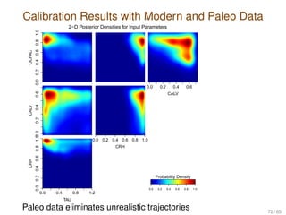
  • 72. Calibration Results with Modern and Paleo Data 0.00.20.40.60.81.0 OCFAC 2−D Posterior Densities for Input Parameters 0.0 0.2 0.4 0.6 CALV 0.00.20.40.6 CALV 0.0 0.2 0.4 0.6 0.8 1.0 CRH 0.0 0.4 0.8 1.2 TAU 0.00.20.40.60.81.0 CRH 0.0 0.2 0.4 0.6 0.8 1.0 Probability Density Paleo data eliminates unrealistic trajectories 72 / 85
  • 73. Why are the Results Different? Unrealistic simulations with overshoots in past ice retreat and projected future regrowth are eliminated This “constrains” the probability distribution of the parameters 73 / 85
  • 74. Ice Volume Projections: Paleo Cuts Off Left Tail 0.00.51.01.52.0 Ice Volume Change Projection (500 years) ice volume change [m sle] probabilitydensity −10 −8 −6 −4 −2 0 1 2 3 4 5 ( ) ( ) current approach modern obs. only no calibration Possibility of “no sea level rise” is virtually eliminated. 74 / 85
  • 75. Multivariate output Very common to have models with multiple outputs. Time series. Spatial or spatio-temporal. Multiple time series, multiple spatial grids. E.g. from climate science. Qualitative and quantitative outputs. cf. (Qiang,Wu,Wu, 2007). Could emulate each output separately though this approach ignores relationships among the outputs. If the relationships are important, need more sophisticated approaches 75 / 85
  • 76. Multivariate output: some approaches Bayarri et al. (2007, 2008): represent output in the form of wavelets. Emulate coefficients. Higdon et al. (2008): reduce dimensionality by looking at principal components. Emulate the first few components. Issue: how loss of information impacts inference/prediction, especially when we are interested in unusual events. Spatial fields: Use Gaussian processes at two levels so GP covariance depends on inputs as well as location of data (Sanso et al., 2008; Bhat et al., 2009). Lots of open problems, e.g. spatio-temporal output, especially if we want to incorporate dynamics well. 76 / 85
  • 77. Design issues: choice of training data points Since computer models are expensive, training data points are generally small in number. Important to select these points carefully. Some design criteria: Spread points over the most ‘interesting’ part of the input space, where predictions are of most interest To learn about covariance function smoothness would also like some points close to each other These are competing criteria. Hence, need a design that strikes a balance. See Zhu and Stein (2005) for a nice study of design for Gaussian process models Often use latin hypercube (LHC) designs, Sobol sequences, Support Points (Mak and Joseph, 2016) SAMSI Quasi-Monte Carlo program this year 77 / 85
  • 78. Research Challenges 1. Increased flexibility. Nonstationarities: smoothness varying over input space. Non-isotropic, emulations which allows for jumps. E.g. Treed Gaussian process (Gramacy and Lee, 2008) 2. Large training data sets. Expensive matrix operations (need ‘sparse’ methods): 3. Dimensionality of input: note that as the dimensionality of inputs increases, need much more training data, which causes problems above. Items (1), (2) are also active areas of research in statistics in the spatial modeling context. 78 / 85
  • 79. More Research Challenges Complicated output: multivariate, time series, spatial, multivariate-spatial, qualitative and quantitative etc. Design, sequential design Dynamic emulation: approximating model runs with inputs that vary over time The MCMC-based approach is time consuming. Alternatives for some cases that are fast? How to characterize model discrepancy, identifiable? Combining information from multiple models: what projection/decision to make in the face of conflicting projections from different models? 79 / 85
  • 80. Combining Information from Multiple Models Average projection (democratic approach) is not ideal Results may be too smooth/unrealistic Average may not be physically meaningful Weighting based on the past (“hindcasts”) Different models may have different projections, but similar hindcasts (they have been tuned to the same data after all!) Re-using the same data sets Hard to determine metrics Particularly challenging for extremes Many open questions. Nice discussions in Knutti et al. (2010); Knutti (2011) 80 / 85
  • 81. Uncertainties Not Quantified... Only truly addressed parametric uncertainty and (some) observational uncertainty, and interpolation uncertainty. How about the others? Structural: perhaps by using multiple models? But the models are not that different (Jun, Knutti, Nychka, 2008). They underestimate model uncertainty Internal/natural climate variability: can approximate this by doing control runs, i.e., run the model without forcings (cf. Sanso, Forest, Zantedeschi, 2008) Boundary or initial condition uncertainty: create initial value ensembles (cf. Sriver et al., 2015) “Forcings” uncertainty, e.g. uncertainty about emissions: very difficult to do this, only study it via case studies 81 / 85
  • 82. Recap What are climate models? Uncertainty quantification, types of uncertainties Focused on parametric uncertainty, hence model calibration Bayesian inference and calibration basics Gaussian processes (GP) for emulation and calibration Extending GPs to emulation-calibration with high-dimensional spatial data and non-Gaussian spatial data Open research problems, e.g. unadressed uncertainties, computational challenges 82 / 85
  • 83. Acknowledgments Rasmussen and Williams (2006) “Gaussian processes for machine learning”. Available online for free! Gaussian processes website Tony O’Hagan’s talks/papers on MUCM projects (Managing Uncertainty in Computer Models) Conversation about climate models with Adam Monahan 83 / 85
  • 84. Collaborators Won Chang, University of Cincinnati Yawen Guan, Penn State Statistics David Pollard, Earth and Environmental Systems Institute (EESI), Penn State U. Patrick Applegate, EESI, Penn State U. Klaus Keller, Geosciences, Penn State U. Roman Olson, The University of New South Wales This work was partially supported by the following grants: The Network for Sustainable Climate Risk Management (SCRiM), NSF GEO-1240507. NSF CDSE/DMS-1418090 Statistical Methods for Ice Sheet Projections 84 / 85
  • 85. References Kennedy, M.C. and O’Hagan, A.( 2001), Bayesian calibration of computer models, JRSS(B) L.M. Berliner (2003) Physical-statistical modeling in geophysics, J. Geophy. Res Chang, W., Haran, M, Applegate, P., Pollard, D. (2016): Improving Ice Sheet Model Calibration Using Paleoclimate and Modern Data, Annals of Applied Statistics Chang, W., Haran, M, Applegate, P., Pollard, D. (2016): Calibrating an Ice sheet model using high-dimensional non-Gaussian spatial data, J of Amer Stat Association Chang, W., M. Haran, R. Olson, and K. Keller (2014): Fast dimension-reduced climate model calibration, Annals of Applied Statistics 85 / 85