Comparison of image segmentation
Download as PPTX, PDF2 likes3,387 views

The document evaluates three image segmentation algorithms: mean shift segmentation, efficient graph-based segmentation, and a hybrid approach combining the first two. It assesses their performance based on correctness, stability with respect to parameter choices, and stability across different images, using the normalized probabilistic rand index for comparison. The findings suggest that the hybrid method offers better stability and performance over a range of parameters compared to the other two algorithms.


Comparison of image segmentation
- 1. Presented by Haitham Abdel-atty Abdullah Yara Bahaa El-Din Hashem Pre-Masters 2014-2015 Supervised by: Prof. Dr. Mostafa Gadal-Haqq 1
- 2. Introduction Image Segmentation Algorithms › Mean Shift Segmentation › Efficient Graph-based Segmentation › Hybrid Segmentation Algorithm Normalized Probabilistic Rand (NPR) Index Experiments Conclusion 2
- 3. Image segmentation Is the process of partitioning a digital image into multiple segments (sets of pixels) The goal of segmentation Is to simplify and/or change the representation of an image into something that is more meaningful and easier to analyze 3
- 4. We will present an evaluation of two popular segmentation algorithms, the mean shift-based segmentation algorithm and a graph-based segmentation scheme. We also consider a hybrid method which combines the other two methods. we compare all use the same image features (position and color) for segmentation, thereby making their outputs directly comparable. 4
- 5. For each of these algorithms, we examine three characteristics: 1. Correctness: the ability to produce results that are consistent with ground truth 2. Stability with respect to parameter choice: the ability to produce segmentations of consistent correctness for a range of parameter choices. 3. Stability with respect to image choice: the ability to produce segmentations of consistent correctness using the same parameter choice on a wide range of different images. The Normalized Probabilistic Rand (NPR) index is used to measure the above characteristics. 5
- 6. 6
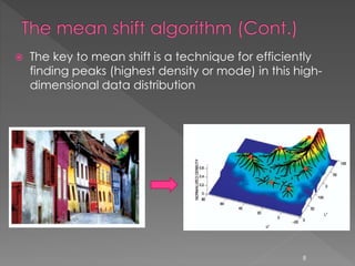
- 7. Is a nonparametric clustering technique which does not require prior knowledge of the number of clusters, and does not constrain the shape of the clusters. Mean shift is used for image segmentation, clustering, visual tracking, space analysis, mode seeking ... Technique for clustering-based segmentation 7
- 8. The key to mean shift is a technique for efficiently finding peaks (highest density or mode) in this high- dimensional data distribution 8
- 9. Density Estimation Gradient Estimation (Mean Shift) Data Discrete PDF Representation (PDF : probability density function) PDF Analysis 9
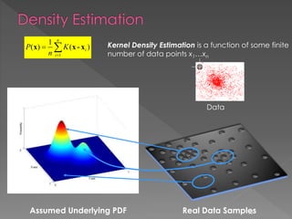
- 10. Assumed Underlying PDF Real Data Samples 1 1 ( ) ( ) n i i P K n x x - x Kernel Density Estimation is a function of some finite number of data points x1…xn Data 10
- 11. Region of interest Center of mass Mean Shift vector 11
- 12. Region of interest Center of mass Mean Shift vector 12
- 13. Region of interest Center of mass Mean Shift vector 13
- 14. Region of interest Center of mass Mean Shift vector 14
- 15. Region of interest Center of mass Mean Shift vector 15
- 16. Region of interest Center of mass Mean Shift vector 16
- 18. 18
- 19. Simple Mean Shift procedure: • Compute mean shift vector •Translate the Kernel window by m(x) 2 1 2 1 ( ) n i i i n i i g h g h x - x x m x x x - x 19
- 20. 20
- 21. Attraction basin: the region for which all trajectories lead to the same peak (mode) Cluster: all data points in the attraction basin of a mode 21
- 22. 22
- 23. 23
- 24. Pros Does not assume spherical clusters Just a single parameter (window size) Robust to outliers Cons Computationally expensive. Have to choose kernel size in advance Output depends on window size. Not suitable for high-dimensional features. 24
- 25. 25
- 26. Another method of performing clustering in feature space. Works on data points in feature space without first performing a filtering step. Key to success of this method is adaptive thresholding. 26
- 27. Represent features and their relationships using a graph Manipulate the graph to segment the image 27
- 28. Node for every pixel Edge between every pair of pixels (or every pair of “sufficiently close” pixels) Each edge is weighted by the similarity of the two nodes wij i j 28
- 29. Break Graph into Segments › Delete links that cross between segments › Easiest to break links that have low affinity similar pixels should be in the same segments dissimilar pixels should be in different segments A B C wij i j 29
- 30. Intensity Color Distance aff x, y exp 1 2i 2 I x I y 2 aff x, y exp 1 2d 2 x y 2 aff x, y exp 1 2t 2 c x c y 2 30
- 31. Small σ: group only nearby points Large σ: group far-away points 31
- 32. Changing scores for different parameters using efficient graph-based segmentation: (a) Original image, (b)-(d) efficient graph-based segmentations using scale bandwidth (hs) 7, color bandwidth (hr) 7 and k values 5, 25, and 125 respectively. 33
- 33. 34
- 34. Combine two previous methods we apply mean shift filtering, and then we use efficient graph-based clustering to give the final segmentation. The quality of the segmentation is high. 35
- 35. Example of changing scores for different parameters using a hybrid segmentation algorithm which first performs mean shift filtering and then efficient graph-based segmentation: (a) Original image, (b)-(g) segmentations using scale bandwidth (hs) 7, and color bandwidth (hr) and k value combinations (3,5), (3,25), (3,125), (15,5), (15,25), (15,125) respectively. 36
- 36. 37
- 37. The Rand index (RI) or Rand measure (named after William M. Rand) is a measure of the similarity between two data clustering. G P a b c d a b c d a a X dcba da GPRI ),( The Rand index has a value between 0 and 1. 38
- 38. The Rand index (RI) a ba + b + c + d RI(P,G) dcba da GPRI ),( 39
- 39. The Probabilistic Rand Index (PRI) counts the fraction of pairs of pixels whose labels are consistent between the computed segmentation and the ground truth, averaging across multiple ground truth (manual) segmentations to account for scale variation in human perception. In other simple words, PRI measuring the similarity between two partitions. 40
- 40. In PRI agreements ( ) and disagreements ( ) at the pixel-pair are weighted according to the probability of their occurring. Computed segmentation Multiple ground truth (manual) segmentations 41
- 41. The PR index does however have one serious flaw. Note that the PR index is on a scale of 0-1, but there is no expected value for a given segmentation. That is, it is impossible to know if any given score is good or bad. The significance of a measure of similarity has much to do with the baseline with respect to which it is expressed. For image segmentation, the baseline may be interpreted as the expected value of the index. All of these issues are resolved with normalization to produce the Normalized Probabilistic Rand (NPR) index Baseline NPR Index Is one PRI 42
- 42. 43
- 43. ‘EDISON’ refers EDISON system for mean shift segmentation. ‘FH’ refers to the efficient graph-based segmentation method. ‘MS+FH’ refers to our hybrid algorithm of mean shift filtering followed by efficient graph-based segmentation. All of the experiments were performed on the publicly available Berkeley image segmentation database which contains 300 images of natural scenes. 44
- 44. Examples of images from the Berkeley image segmentation database 45
- 45. we will divide each dimension by the corresponding {hs, hr} as in the EDISON system. So each algorithm was run with a parameter combination from the sets: hs = 7, hr = {3, 7, 11, 15, 19, 23}, and k = {5, 25, 50, 75, 100, 125}. 46
- 46. Maximum NPR indices achieved on individual images with the set of parameters used for each algorithm. Plot (a) shows the indices achieved on each image individually, ordered by increasing index. Plot (b) shows the same information in the form of a histogram. 47
- 47. All of the algorithms produce similar maximum NPR indices, demonstrating that they have roughly equal ability to produce correct segmentations with the parameter set chosen. Few images which have below-zero maximum NPR index. 48
- 48. An algorithm which creates good segmentations will have a histogram skewed to the right. A standard deviation histogram that is skewed to the left indicates that the algorithm in question is less sensitive to changes in its parameters. Using the means as a measure certainly makes us more dependent on our choice of parameters for each algorithm. 49
- 49. Average performance over all parameter combinations: › Mean NPR plots for each of the three systems with averages taken over all possible combinations of the parameters hr and k 50
- 50. 51
- 51. Mean NPR indices achieved using each of the segmentation algorithms. The first row shows results from the mean shift-based system (EDISON), the second from the efficient graph-based system (FH), and the third from the hybrid segmentation system (MS+FH). Results from each algorithm are given for individual images over the parameter set of all combinations of hr = {3, 7, 11, 15, 19, 23} and k = {5, 25, 50, 75, 100, 125}. Plots (a), (d) and (g) show the mean indices achieved on each image individually, ordered by increasing index, along with one standard deviation. Plots (b), (e) and (h) show histograms of the means. Plots (c), (f) and (i) show histograms of the standard deviations. 52
- 52. Average performance over different values of the color bandwidth hr: › NPR indices averaged over values of hr, with k held constant 53
- 53. 54
- 54. Mean NPR indices achieved using the efficient graph-based segmentation system (FH) on individual images over the parameter set hr = {3, 7, 11, 15, 19, 23} with a constant k. Plot (a) shows the mean indices achieved on each image individually, ordered by increasing index, along with one standard deviation. Plot (b) shows a histogram of the means. Plot (c) shows a histogram of the standard deviations. 55
- 55. 56
- 56. Mean NPR indices achieved using the hybrid segmentation system (MS+FH) on individual images over the parameter set hr = {3, 7, 11, 15, 19, 23} with a constant k. Plot (a) shows the mean indices achieved on each image individually, ordered by increasing index, along with one standard deviation. Plot (b) shows a histogram of the means. Plot (c) shows a histogram of the standard deviations. 57
- 57. Average performance over different values of k › Mean NPR indices as k is varied and hr is held constant. 58
- 58. 59
- 59. Mean NPR indices achieved using the efficient graph-based segmentation system (FH) on individual images over the parameter set k = {5, 25, 50, 75, 100, 125} with a constant hr. Plots (a), (d) and (g) show the mean indices achieved on each image individually, ordered by increasing index, along with one standard deviation. Plots (b), (e) and (h) show histograms of the means. Plots (c), (f) and (i) show histograms of the standard deviations. 60
- 60. 61
- 61. Mean NPR indices achieved using the hybrid segmentation system (MS+FH) on individual images over the parameter set k = {5, 25, 50, 75, 100, 125} with a constant hr. Plots (a), (d) and (g) show the mean indices achieved on each image individually, ordered by increasing index, along with one standard deviation. Plots (b), (e) and (h) show histograms of the means. Plots (c), (f) and (i) show histograms of the standard deviations. 62
- 62. The final set of experiments looks at the stability of a particular parameter combination across images. In each experiment results are shown with respect to a particular parameter, with averages and standard deviations taken over segmentations of each image in the entire image database. 63
- 63. Average performance over all images for different values of hr: Mean NPR indices using the EDISON segmentation system on each color bandwidth (hr) over the set of images, with one standard deviation. 64
- 64. Mean NPR indices using graph-based segmentation (FH) on each color bandwidth hr= {3, 7, 11, 15, 19, 23} over the set of images. One plot per value of k. 65
- 65. Mean NPR indices using hybrid segmentation (MS+FH) on each color bandwidth hr= {3, 7, 11, 15, 19, 23} over the set of images. One plot per value of k. 66
- 66. Average performance over all images for different values of k › Examine the stability of k over a set of images. 67
- 67. Mean NPR indices using efficient graph-based segmentation (FH) on each of k = {5, 25, 50, 75, 100, 125} over the set of images. One plot per value of hr. 68
- 68. Mean NPR indices using hybrid segmentation (MS+FH) on each of k = {5, 25, 50, 75, 100, 125} over the set of images. One plot per value of hr. 69
- 69. The first comparison considered the correctness of the three algorithms. Hybrid algorithm performed slightly better than the mean shift algorithm, and both performed significantly better than the graph-based segmentation. We can conclude that the mean shift filtering step is indeed useful, and that the most promising algorithms are the mean shift segmentation and the hybrid algorithm. 70
- 70. The second comparison considered stability with respect to parameters. The hybrid algorithm showed less variability when its parameters were changed than the mean shift segmentation algorithm. Although the amount of improvement did decline with increasing values of k, the rate of decline was very slow. Although the graph-based segmentation did show very low variability with k = 5, changing the value of k decreased its stability drastically. 71
- 71. Finally, we compared the stability of a particular parameter choice over the set of images. Once again we see that the graph-based algorithm has low variability when k = 5, however its performance and stability decrease rapidly with changing values of k. The comparison between the mean shift segmentation and the hybrid method is much closer here, with neither performing significantly better. 72
- 72. For the three characteristics measured, we have demonstrated that both the mean shift segmentation and hybrid segmentation algorithms can create realistic segmentations with a wide variety of parameters. However the hybrid algorithm has slightly improved stability. Thus, we would choose to incorporate the hybrid method into a larger system. 73