


![9
Matrix-chain Multiplication …
• To compute the number of scalar multiplications
necessary, we must know:
- Algorithm to multiply two matrices, matrix dimensions
Input: Matrices Ap×q
and Bq×r
(with dimensions p×q and q×r)
Result: Matrix Cp×r
resulting from the product A·B
MATRIX-MULTIPLY(Ap×q
, Bq×r
)
1. for i ← 1 to p
2. for j ← 1 to r
3. C[i, j] ← 0
4. for k ← 1 to q
5. C[i, j] ← C[i, j] + A[i, k] · B[k, j]
6. return C
Scalar multiplication in line 5 dominates time to compute C
Number of scalar multiplications = pqr](https://image.slidesharecdn.com/segment3-230220032319-706e6f57/85/Computer-algorithm-Dynamic-Programming-pdf-9-320.jpg)


![13
Matrix-chain Multiplication …
2. Recursive definition of the value of an optimal
solution
– Let m[i, j] be the minimum number of scalar
multiplications necessary to compute Ai..j
– Minimum cost to compute A1..n
is m[1, n]
– Suppose the optimal parenthesization of Ai..j
splits
the product between Ak
and Ak+1
for some integer k
where i ≤ k < j](https://image.slidesharecdn.com/segment3-230220032319-706e6f57/85/Computer-algorithm-Dynamic-Programming-pdf-13-320.jpg)
![14
Matrix-chain Multiplication …
– Ai..j
= (Ai
Ai+1
…Ak
)·(Ak+1
Ak+2
…Aj
)= Ai..k
· Ak+1..j
– Cost of computing Ai..j
= cost of computing Ai..k
+
cost of computing Ak+1..j
+ cost of multiplying Ai..k
and Ak+1..j
– Cost of multiplying Ai..k
and Ak+1..j
is pi-1
pk
pj
– m[i, j ] = m[i, k] + m[k+1, j ] + pi-1
pk
pj
for i ≤ k < j
– m[i, i ] = 0 for i=1,2,…,n
– But… optimal parenthesization occurs at one
value of k among all possible i ≤ k < j
– Check all these and select the best one](https://image.slidesharecdn.com/segment3-230220032319-706e6f57/85/Computer-algorithm-Dynamic-Programming-pdf-14-320.jpg)
![15
Matrix-chain Multiplication …
m[i, j ] =
0 if i=j
min {m[i, k] + m[k+1, j ] + pi-1
pk
pj
} if i<j
i ≤ k< j
• To keep track of how to construct an optimal solution,
we use a table s
• s[i, j ] = value of k at which Ai
Ai+1
… Aj
is split for
optimal parenthesization
• Algorithm: next slide
– First computes costs for chains of length l=1
– Then for chains of length l=2,3, … and so on
– Computes the optimal cost bottom-up](https://image.slidesharecdn.com/segment3-230220032319-706e6f57/85/Computer-algorithm-Dynamic-Programming-pdf-15-320.jpg)
![16
Matrix-chain Multiplication …
Input: Array p[0…n] containing matrix dimensions and n
Result: Minimum-cost table m and split table s
MATRIX-CHAIN-ORDER(p[ ], n)
for i ← 1 to n
m[i, i] ← 0
for l ← 2 to n
for i ← 1 to n-l+1
j ← i+l-1
m[i, j] ← ∞
for k ← i to j-1
q ← m[i, k] + m[k+1, j] + p[i-1] p[k] p[j]
if q < m[i, j]
m[i, j] ← q
s[i, j] ← k
return m and s
Takes O(n3
) time
Requires O(n2
) space
3. Computing the optimal costs](https://image.slidesharecdn.com/segment3-230220032319-706e6f57/85/Computer-algorithm-Dynamic-Programming-pdf-16-320.jpg)
![17
Matrix-chain Multiplication …
Print-Optimal-Parens(s, i, j)
1. {
2. if i = j
3. then print “Ai
” :
4. else
5. { print “(”;
6. Print-Optimal-Parens(s, i, s[i, j]);
7. Print-Optimal-Parens(s, s[i, j]+1, j);
8. print “)” ;
9. }
10. }
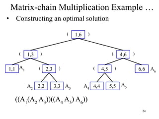
4. Constructing an optimal solution](https://image.slidesharecdn.com/segment3-230220032319-706e6f57/85/Computer-algorithm-Dynamic-Programming-pdf-17-320.jpg)
![18
Matrix-chain Multiplication Example
Matrix Dimension
A1
30×35
A2
35×15
A3
15×5
A4
5×10
A5
10×20
A6
20×25
Assign
p0
=30
p1
=35
p2
=15
p3
=5
p4
=10
p5
=20
p6
=25
m[i,i]
m[1,1]=0
m[2,2]=0
m[3,3]=0
m[4,4]=0
m[5,5]=0
m[6,6]=0](https://image.slidesharecdn.com/segment3-230220032319-706e6f57/85/Computer-algorithm-Dynamic-Programming-pdf-18-320.jpg)
![19
Matrix-chain Multiplication Example …
m[1,2]=m[1,1] + m[2,2] + p0
p1
p2
=0+0+30.35.15=15750
m[2,3]=m[2,2] + m[3,3] + p1
p2
p3
=0+0+35.15.5=2625
m[3,4]=m[3,3] + m[4,4] + p2
p3
p4
=0+0+15.5.10=750
m[4,5]=m[4,4] + m[5,5] + p3
p4
p5
=0+0+5.10.20=1000
m[5,6]=m[5,5] + m[6,6] + p4
p5
p6
=0+0+10.20.25=5000
m i
j
1 2 3 4 5 6
6 5000 0
5 1000 0
4 750 0
3 2625 0
2 15750 0
1 0
s i (value of k)
j
1 2 3 4 5
6 5
5 4
4 3
3 2
2 1](https://image.slidesharecdn.com/segment3-230220032319-706e6f57/85/Computer-algorithm-Dynamic-Programming-pdf-19-320.jpg)
![20
Matrix-chain Multiplication Example …
m[1,3]=min
m[1,1] + m[2,3] + p0
p1
p3
=7875
m i
j
1 2 3 4 5 6
6 3500 5000 0
5 2300 1000 0
4 4375 750 0
3 7875 2625 0
2 15750 0
1 0
s i (value of k)
j
1 2 3 4 5
6 5 5
5 3 4
4 3 3
3 1 2
2 1
m[1,2] + m[3,3] + p0
p2
p3
=18000
m[2,4]=min ? m[3,5]=min ? m[4,6]=min ?](https://image.slidesharecdn.com/segment3-230220032319-706e6f57/85/Computer-algorithm-Dynamic-Programming-pdf-20-320.jpg)
![21
Matrix-chain Multiplication Example …
m[1,4]=min
m[1,1] + m[2,4] + p0
p1
p4
=?
m i
j
1 2 3 4 5 6
6 5375 3500 5000 0
5 7125 2300 1000 0
4 9375 4375 750 0
3 7875 2625 0
2 15750 0
1 0
s i (value of k)
j
1 2 3 4 5
6 3 5 5
5 3 3 4
4 3 3 3
3 1 2
2 1
m[1,2] + m[3,4] + p0
p2
p4
=?
m[2,5]=min ? m[3,6]=min ?
m[1,3] + m[4,4] + p0
p3
p4
=9375](https://image.slidesharecdn.com/segment3-230220032319-706e6f57/85/Computer-algorithm-Dynamic-Programming-pdf-21-320.jpg)
![22
Matrix-chain Multiplication Example …
m[1,5]=min
m[1,1] + m[2,5] + p0
p1
p5
=?
m i
j
1 2 3 4 5 6
6 10500 5375 3500 5000 0
5 11875 7125 2300 1000 0
4 9375 4375 750 0
3 7875 2625 0
2 15750 0
1 0
s i (value of k)
j
1 2 3 4 5
6 3 3 5 5
5 3 3 3 4
4 3 3 3
3 1 2
2 1
m[1,2] + m[3,5] + p0
p2
p5
=?
m[2,6]=min
?
m[1,3] + m[4,5] + p0
p3
p5
=11875
m[1,4] + m[5,5] + p0
p4
p5
=?](https://image.slidesharecdn.com/segment3-230220032319-706e6f57/85/Computer-algorithm-Dynamic-Programming-pdf-22-320.jpg)
![23
23
Matrix-chain Multiplication Example …
m[1,6]=min
m[1,1] + m[2,6] + p0
p1
p6
=?
m i
j
1 2 3 4 5 6
6 15125 10500 5375 3500 5000 0
5 11875 7125 2500 1000 0
4 9375 4375 750 0
3 7875 2625 0
2 15750 0
1 0
s i (value of k)
j
1 2 3 4 5
6 3 3 3 5 5
5 3 3 3 4
4 3 3 3
3 1 2
2 1
m[1,2] + m[3,6] + p0
p2
p6
=?
m[1,3] + m[4,6] + p0
p3
p6
=15125
m[1,4] + m[5,6] + p0
p4
p6
=?
m[1,5] + m[6,6] + p0
p5
p6
=?](https://image.slidesharecdn.com/segment3-230220032319-706e6f57/85/Computer-algorithm-Dynamic-Programming-pdf-23-320.jpg)


![33
A recursive solution to subproblems …
Like the matrix-chain multiplication problem, our recursive
solution to the LCS problem involves establishing a recurrence
of the cost of an optimal solution. Let us define c[i,j] to be the
length of an LCS of the sequences Xi
, and Yj
. If either i = 0 or j
= 0, one of the sequences has length 0, so the LCS has length 0.
The optimal substructure of the LCS problem gives the
recursive formula
0 if i = 0 or j = 0
c[i,j] = c[i-1, j-1]+1 if i, j > 0 and xi
= yj
max(c[i,j-1], c[i-1,j]) if i, j > 0 and xi
≠ yj](https://image.slidesharecdn.com/segment3-230220032319-706e6f57/85/Computer-algorithm-Dynamic-Programming-pdf-33-320.jpg)
![34
Computing the length of an LCS
Based on recursive equation, we could easily write an
exponential-time recursive algorithm to compute the length of
an LCS of two sequences. Since there are only Θ(mn) distinct
subproblems, however, we can use dynamic programming to
compute the solutions bottom up.
Procedure LCS-LENGTH takes two sequences X = <x1
, x2
,
…, xm
> and Y = <y1
, y2
, …, yn
> as inputs. It stores the c[i,j]
values in a table c[0..m,0..n] whose entries are computed in
row-major order. (That is, the first row of c is filled in form left
to right, then the second row, and so on.) It also maintains the
table b[1.m,1..n] to simplify construction of an optimal solution.
Intuitively, b[i,j] points to the table entry corresponding to the
optimal subproblem solution chosen when computing b[i,j]. The
procedure returns the b and c tables: c[m,n] contains the length
of an LCS of X and Y.](https://image.slidesharecdn.com/segment3-230220032319-706e6f57/85/Computer-algorithm-Dynamic-Programming-pdf-34-320.jpg)
![35
LCS-LENGTH (X, Y)
1. m ← length[X]
2. n ← length[Y]
3. for i ← 1 to m
4. do c[i, 0] ← 0
5. for j ← 0 to n
6. do c[0, j ] ← 0
7. for i ← 1 to m
8. do for j ← 1 to n
9. do if xi
= yj
10. then c[i, j ] ← c[i−1, j−1] + 1
11. b[i, j ] ← “ ”
12. else if c[i−1, j ] ≥ c[i, j−1]
13. then c[i, j ] ← c[i− 1, j ]
14. b[i, j ] ← “↑”
15. else c[i, j ] ← c[i, j−1]
16. b[i, j ] ← “←”
17. return c and b
Computing the length of an LCS ….
b[i, j ] points to table
entry whose
subproblem we used in
solving LCS of Xi
and Yj
.
c[m,n] contains the
length of an LCS of X
and Y.](https://image.slidesharecdn.com/segment3-230220032319-706e6f57/85/Computer-algorithm-Dynamic-Programming-pdf-35-320.jpg)

![37
Figure 3.1 The c and b tables computed by LCS-LENGTH on
the sequence X=<A, B, C, B, D, A, B> and Y=<B, D, C, A, B,
A>. The square in row i and column j contains the value of
c[i,j] and the appropriate arrow for the value of b[i,j]. The
entry 4 in c[7,4]– the lower right-hand corner of the table—is
the length of an LCS <B, C, B, A> of X and Y. For i,j > 0,
entry c[i,j] depends only on whether xi
= yi
and the values in
entries c[i-1,j],c[i,j-1], and c[i-1,j-1], which are computed
before c[i,j]. To reconstruct the elements of an LCS, follow the
b[i,j] arrows from the lower right-hand corner; the path is
shaded. Each “ ” on the path corresponds to an entry
(highlighted) for which xi
= yi
is a member of an LCS
Computing the length of an LCS ….](https://image.slidesharecdn.com/segment3-230220032319-706e6f57/85/Computer-algorithm-Dynamic-Programming-pdf-37-320.jpg)

![39
Construction an LCS
The b table returned by LCS-LENGTH can be to quickly
construct an LCS of X = <x1
, x2
, …, xm
> and Y = <y1
, y2
, …,
yn
>. We simply begin at b[m,n] and trace through the table
following the arrows. Whenever we encounter a “ ” in entry
b[i,j], it implies that xi
= yj
is an element of the LCS. The
elements of the LCS are encountered in reverse order by this
method. The following recursive procedure prints out an LCS of
X and Y in the proper, forward order. The initial invocation is
PRINT-LCS(b, X, length[x], lentgh[Y]).](https://image.slidesharecdn.com/segment3-230220032319-706e6f57/85/Computer-algorithm-Dynamic-Programming-pdf-39-320.jpg)
![40
Construction an LCS…..
PRINT-LCS (b, X, i, j)
1. if i = 0 or j = 0
2. then return
3. if b[i, j ] = “ ”
4. then PRINT-LCS(b, X, i−1, j−1)
5. print xi
6. elseif b[i, j ] = “↑”
7. then PRINT-LCS(b, X, i−1, j)
8. else PRINT-LCS(b, X, i, j−1)
•Initial call is PRINT-LCS (b, X,m, n).
•When b[i, j ] = , we have extended LCS by one character. So
LCS = entries with in them.
•Time: O(m+n)](https://image.slidesharecdn.com/segment3-230220032319-706e6f57/85/Computer-algorithm-Dynamic-Programming-pdf-40-320.jpg)


![43
LCS Example (0)
0
1
2
3
4
i
X
i
A
B
C
B
Y
j
B
B A
C
D
X = ABCB; m = |X| = 4
Y = BDCAB; n = |Y| = 5
Allocate array c[5,4]
ABCB
BDCAB
j 0 1 2 3 4 5](https://image.slidesharecdn.com/segment3-230220032319-706e6f57/85/Computer-algorithm-Dynamic-Programming-pdf-43-320.jpg)
![44
LCS Example (1)
j 0 1 2 3 4 5
0
1
2
3
4
i
X
i
A
B
C
B
Y
j
B
B A
C
D
0
0
0
0
0
0
0
0
0
0
for i = 1 to m c[i,0] = 0
for j = 1 to n c[0,j] = 0
ABCB
BDCAB](https://image.slidesharecdn.com/segment3-230220032319-706e6f57/85/Computer-algorithm-Dynamic-Programming-pdf-44-320.jpg)
![12/25/2022 45
LCS Example (2)
0
1
2
3
4
i
X
i
A
B
C
B
Y
j
B
B A
C
D
0
0
0
0
0
0
0
0
0
0
if ( Xi
== Yj
)
c[i,j] = c[i-1,j-1] + 1
else c[i,j] = max( c[i-1,j], c[i,j-1] )
0
ABCB
BDCAB
j 0 1 2 3 4 5](https://image.slidesharecdn.com/segment3-230220032319-706e6f57/85/Computer-algorithm-Dynamic-Programming-pdf-45-320.jpg)
![12/25/2022 46
LCS Example (3)
0
1
2
3
4
i
X
i
A
B
C
B
Y
j
B
B A
C
D
0
0
0
0
0
0
0
0
0
0
if ( Xi
== Yj
)
c[i,j] = c[i-1,j-1] + 1
else c[i,j] = max( c[i-1,j], c[i,j-1] )
0 0 0
ABCB
BDCAB
j 0 1 2 3 4 5](https://image.slidesharecdn.com/segment3-230220032319-706e6f57/85/Computer-algorithm-Dynamic-Programming-pdf-46-320.jpg)
![12/25/2022 47
LCS Example (4)
0
1
2
3
4
i
X
i
A
B
C
B
Y
j
B
B A
C
D
0
0
0
0
0
0
0
0
0
0
if ( Xi
== Yj
)
c[i,j] = c[i-1,j-1] + 1
else c[i,j] = max( c[i-1,j], c[i,j-1] )
0 0 0 1
ABCB
BDCAB
j 0 1 2 3 4 5](https://image.slidesharecdn.com/segment3-230220032319-706e6f57/85/Computer-algorithm-Dynamic-Programming-pdf-47-320.jpg)
![12/25/2022 48
LCS Example (5)
0
1
2
3
4
i
X
i
A
B
C
B
Y
j
B
B A
C
D
0
0
0
0
0
0
0
0
0
0
if ( Xi
== Yj
)
c[i,j] = c[i-1,j-1] + 1
else c[i,j] = max( c[i-1,j], c[i,j-1] )
0
0
0 1 1
ABCB
BDCAB
j 0 1 2 3 4 5](https://image.slidesharecdn.com/segment3-230220032319-706e6f57/85/Computer-algorithm-Dynamic-Programming-pdf-48-320.jpg)
![12/25/2022 49
LCS Example (6)
0
1
2
3
4
i
X
i
A
B
C
B
Y
j
B
B A
C
D
0
0
0
0
0
0
0
0
0
0
if ( Xi
== Yj
)
c[i,j] = c[i-1,j-1] + 1
else c[i,j] = max( c[i-1,j], c[i,j-1] )
0 0 1
0 1
1
ABCB
BDCAB
j 0 1 2 3 4 5](https://image.slidesharecdn.com/segment3-230220032319-706e6f57/85/Computer-algorithm-Dynamic-Programming-pdf-49-320.jpg)
![12/25/2022 50
LCS Example (7)
0
1
2
3
4
i
X
i
A
B
C
B
Y
j
B
B A
C
D
0
0
0
0
0
0
0
0
0
0
if ( Xi
== Yj
)
c[i,j] = c[i-1,j-1] + 1
else c[i,j] = max( c[i-1,j], c[i,j-1] )
1
0
0
0 1
1 1 1
1
ABCB
BDCAB
j 0 1 2 3 4 5](https://image.slidesharecdn.com/segment3-230220032319-706e6f57/85/Computer-algorithm-Dynamic-Programming-pdf-50-320.jpg)
![12/25/2022 51
LCS Example (8)
0
1
2
3
4
i
X
i
A
B
C
B
Y
j
B
B A
C
D
0
0
0
0
0
0
0
0
0
0
if ( Xi
== Yj
)
c[i,j] = c[i-1,j-1] + 1
else c[i,j] = max( c[i-1,j], c[i,j-1] )
1
0
0
0 1
1 1 1 1 2
ABCB
BDCAB
j 0 1 2 3 4 5](https://image.slidesharecdn.com/segment3-230220032319-706e6f57/85/Computer-algorithm-Dynamic-Programming-pdf-51-320.jpg)
![12/25/2022 52
LCS Example (10)
0
1
2
3
4
i
X
i
A
B
C
B
Y
j
B
B A
C
D
0
0
0
0
0
0
0
0
0
0
if ( Xi
== Yj
)
c[i,j] = c[i-1,j-1] + 1
else c[i,j] = max( c[i-1,j], c[i,j-1] )
1
0
0
0 1
2
1 1 1
1
1 1
ABCB
BDCAB
j 0 1 2 3 4 5](https://image.slidesharecdn.com/segment3-230220032319-706e6f57/85/Computer-algorithm-Dynamic-Programming-pdf-52-320.jpg)
![12/25/2022 53
LCS Example (11)
0
1
2
3
4
i
X
i
A
B
C
B
Y
j
B
B A
C
D
0
0
0
0
0
0
0
0
0
0
if ( Xi
== Yj
)
c[i,j] = c[i-1,j-1] + 1
else c[i,j] = max( c[i-1,j], c[i,j-1] )
1
0
0
0 1
1 2
1 1
1
1 1 2
ABCB
BDCAB
j 0 1 2 3 4 5](https://image.slidesharecdn.com/segment3-230220032319-706e6f57/85/Computer-algorithm-Dynamic-Programming-pdf-53-320.jpg)
![12/25/2022 54
LCS Example (12)
0
1
2
3
4
i
X
i
A
B
C
B
Y
j
B
B A
C
D
0
0
0
0
0
0
0
0
0
0
if ( Xi
== Yj
)
c[i,j] = c[i-1,j-1] + 1
else c[i,j] = max( c[i-1,j], c[i,j-1] )
1
0
0
0 1
1 2
1 1
1 1 2
1
2
2
ABCB
BDCAB
j 0 1 2 3 4 5](https://image.slidesharecdn.com/segment3-230220032319-706e6f57/85/Computer-algorithm-Dynamic-Programming-pdf-54-320.jpg)
![12/25/2022 55
LCS Example (13)
0
1
2
3
4
i
X
i
A
B
C
B
Y
j
B
B A
C
D
0
0
0
0
0
0
0
0
0
0
if ( Xi
== Yj
)
c[i,j] = c[i-1,j-1] + 1
else c[i,j] = max( c[i-1,j], c[i,j-1] )
1
0
0
0 1
1 2
1 1
1 1 2
1
2
2
1
ABCB
BDCAB
j 0 1 2 3 4 5](https://image.slidesharecdn.com/segment3-230220032319-706e6f57/85/Computer-algorithm-Dynamic-Programming-pdf-55-320.jpg)
![12/25/2022 56
LCS Example (14)
0
1
2
3
4
i
X
i
A
B
C
B
Y
j
B
B A
C
D
0
0
0
0
0
0
0
0
0
0
if ( Xi
== Yj
)
c[i,j] = c[i-1,j-1] + 1
else c[i,j] = max( c[i-1,j], c[i,j-1] )
1
0
0
0 1
1 2
1 1
1 1 2
1
2
2
1 1 2 2
ABCB
BDCAB
j 0 1 2 3 4 5](https://image.slidesharecdn.com/segment3-230220032319-706e6f57/85/Computer-algorithm-Dynamic-Programming-pdf-56-320.jpg)
![12/25/2022 57
LCS Example (15)
0
1
2
3
4
i
X
i
A
B
C
B
Y
j
B
B A
C
D
0
0
0
0
0
0
0
0
0
0
if ( Xi
== Yj
)
c[i,j] = c[i-1,j-1] + 1
else c[i,j] = max( c[i-1,j], c[i,j-1] )
1
0
0
0 1
1 2
1 1
1 1 2
1
2
2
1 1 2 2 3
ABCB
BDCAB
j 0 1 2 3 4 5](https://image.slidesharecdn.com/segment3-230220032319-706e6f57/85/Computer-algorithm-Dynamic-Programming-pdf-57-320.jpg)


Ad
More Related Content
Similar to Computer algorithm(Dynamic Programming).pdf (20)
Recently uploaded (20)


Ad
Computer algorithm(Dynamic Programming).pdf
- 1. 1 Computer Algorithms Segment 3 Dynamic Programming
- 2. 2 Why Dynamic Programming? • Divide-and-Conquer: a top-down approach. Many smaller instances are computed more than once. • Dynamic programming: a bottom-up approach. Solutions for smaller instances are stored in a table for later use. • It sometimes happens that the natural way of dividing an instance suggested by the structure of the problem leads us to consider several overlapping subinstances. • If we solve each of these independently, they will in turn create a large number of identical subinstances.
- 3. 3 Why Dynamic Programming?.... • If we pay no attention to this duplication, it is likely that we will end up with an inefficient algorithm. • If, on the other hand, we take advantage of the duplication and solve each subinstance only once, saving the solution for later use, then a more efficient algorithm will result. • The underlying idea of dynamic programming is thus quite simple: avoid calculating the same thing twice, usually by keeping a table of known results, which we fill up as subinstances are solved. • Dynamic programming is a bottom-up technique.
- 4. 4 What is Dynamic Programming? • Dynamic Programming is a general algorithm design technique. • Invented by American mathematician Richard Bellman in the 1950s to solve optimization problems. • “Programming” here means “planning”. • Main idea: • solve several smaller (overlapping) subproblems. • record solutions in a table so that each subproblem is only solved once. • final state of the table will be (or contain) solution.
- 5. 5 What is Dynamic Programming?... • Dynamic programming solves optimization problems by combining solutions to subproblems • “Programming” refers to a tabular method with a series of choices, not “coding” • A set of choices must be made to arrive at an optimal solution • As choices are made, subproblems of the same form arise frequently • The key is to store the solutions of subproblems to be reused in the future
- 6. 6 What is Dynamic Programming? ... • Recall the divide-and-conquer approach – Partition the problem into independent subproblems – Solve the subproblems recursively – Combine solutions of subproblems • This contrasts with the dynamic programming approach • Dynamic programming is applicable when subproblems are not independent – i.e., subproblems share subsubproblems – Solve every subsubproblem only once and store the answer for use when it reappears • A divide-and-conquer approach will do more work than necessary
- 7. 7 Elements of Dynamic Programming? • Development of a dynamic programming solution to an optimization problem involves four steps 1. Characterize the structure of an optimal solution - Optimal substructures, where an optimal solution consists of sub-solutions that are optimal. - Overlapping sub-problems where the space of sub-problems is small in the sense that the algorithm solves the same sub-problems over and over rather than generating new sub-problems. 2. Recursively define the value of an optimal solution. - define the value of an optimal solution based on value of solutions to sub-problems. 3. Compute the value of an optimal solution in a bottom-up manner. - compute in a bottom-up fashion and save the values along the way - later steps use the save values of pervious steps 4. Construct an optimal solution from the computed optimal
- 8. 8 Matrix-chain Multiplication • Suppose we have a sequence or chain A1 , A2 , …, An of n matrices to be multiplied – That is, we want to compute the product A1 A2 …An • There are many possible ways (parenthesizations) to compute the product • Example: consider the chain A1 , A2 , A3 , A4 of 4 matrices – Let us compute the product A1 A2 A3 A4 • There are 5 possible ways: 1. (A1 (A2 (A3 A4 ))) 2. (A1 ((A2 A3 )A4 )) 3. ((A1 A2 )(A3 A4 )) 4. ((A1 (A2 A3 ))A4 ) 5. (((A1 A2 )A3 )A4 )
- 9. 9 Matrix-chain Multiplication … • To compute the number of scalar multiplications necessary, we must know: - Algorithm to multiply two matrices, matrix dimensions Input: Matrices Ap×q and Bq×r (with dimensions p×q and q×r) Result: Matrix Cp×r resulting from the product A·B MATRIX-MULTIPLY(Ap×q , Bq×r ) 1. for i ← 1 to p 2. for j ← 1 to r 3. C[i, j] ← 0 4. for k ← 1 to q 5. C[i, j] ← C[i, j] + A[i, k] · B[k, j] 6. return C Scalar multiplication in line 5 dominates time to compute C Number of scalar multiplications = pqr
- 10. 10 Matrix-chain Multiplication … • Example: Consider three matrices A10×100 , B100×5 , and C5×50 • There are 2 ways to parenthesize – ((AB)C) = D10×5 · C5×50 • AB ⇒ 10·100·5=5,000 scalar multiplications • DC ⇒ 10·5·50 =2,500 scalar multiplications – (A(BC)) = A10×100 · E100×50 • BC ⇒ 100·5·50=25,000 scalar multiplications • AE ⇒ 10·100·50 =50,000 scalar multiplications Total: 7,500 Total: 75,000
- 11. 11 Matrix-chain Multiplication … • Matrix-chain multiplication problem – Given a chain A1 , A2 , …, An of n matrices, where for i=1, 2, …, n, matrix Ai has dimension pi-1 ×pi – Parenthesize the product A1 A2 …An such that the total number of scalar multiplications is minimized
- 12. 12 Matrix-chain Multiplication … 1. The structure of an optimal solution – Let us use the notation Ai..j for the matrix that results from the product Ai Ai+1 … Aj – An optimal parenthesization of the product A1 A2 …An splits the product between Ak and Ak+1 for some integer k where1 ≤ k < n – First compute matrices A1..k and Ak+1..n ; then multiply them to get the final matrix A1..n – Key observation: parenthesizations of the subchains A1 A2 …Ak and Ak+1 Ak+2 …An must also be optimal if the parenthesization of the chain A1 A2 …An is optimal (why?) – That is, the optimal solution to the problem contains within it the optimal solution to subproblems
- 13. 13 Matrix-chain Multiplication … 2. Recursive definition of the value of an optimal solution – Let m[i, j] be the minimum number of scalar multiplications necessary to compute Ai..j – Minimum cost to compute A1..n is m[1, n] – Suppose the optimal parenthesization of Ai..j splits the product between Ak and Ak+1 for some integer k where i ≤ k < j
- 14. 14 Matrix-chain Multiplication … – Ai..j = (Ai Ai+1 …Ak )·(Ak+1 Ak+2 …Aj )= Ai..k · Ak+1..j – Cost of computing Ai..j = cost of computing Ai..k + cost of computing Ak+1..j + cost of multiplying Ai..k and Ak+1..j – Cost of multiplying Ai..k and Ak+1..j is pi-1 pk pj – m[i, j ] = m[i, k] + m[k+1, j ] + pi-1 pk pj for i ≤ k < j – m[i, i ] = 0 for i=1,2,…,n – But… optimal parenthesization occurs at one value of k among all possible i ≤ k < j – Check all these and select the best one
- 15. 15 Matrix-chain Multiplication … m[i, j ] = 0 if i=j min {m[i, k] + m[k+1, j ] + pi-1 pk pj } if i<j i ≤ k< j • To keep track of how to construct an optimal solution, we use a table s • s[i, j ] = value of k at which Ai Ai+1 … Aj is split for optimal parenthesization • Algorithm: next slide – First computes costs for chains of length l=1 – Then for chains of length l=2,3, … and so on – Computes the optimal cost bottom-up
- 16. 16 Matrix-chain Multiplication … Input: Array p[0…n] containing matrix dimensions and n Result: Minimum-cost table m and split table s MATRIX-CHAIN-ORDER(p[ ], n) for i ← 1 to n m[i, i] ← 0 for l ← 2 to n for i ← 1 to n-l+1 j ← i+l-1 m[i, j] ← ∞ for k ← i to j-1 q ← m[i, k] + m[k+1, j] + p[i-1] p[k] p[j] if q < m[i, j] m[i, j] ← q s[i, j] ← k return m and s Takes O(n3 ) time Requires O(n2 ) space 3. Computing the optimal costs
- 17. 17 Matrix-chain Multiplication … Print-Optimal-Parens(s, i, j) 1. { 2. if i = j 3. then print “Ai ” : 4. else 5. { print “(”; 6. Print-Optimal-Parens(s, i, s[i, j]); 7. Print-Optimal-Parens(s, s[i, j]+1, j); 8. print “)” ; 9. } 10. } 4. Constructing an optimal solution
- 18. 18 Matrix-chain Multiplication Example Matrix Dimension A1 30×35 A2 35×15 A3 15×5 A4 5×10 A5 10×20 A6 20×25 Assign p0 =30 p1 =35 p2 =15 p3 =5 p4 =10 p5 =20 p6 =25 m[i,i] m[1,1]=0 m[2,2]=0 m[3,3]=0 m[4,4]=0 m[5,5]=0 m[6,6]=0
- 19. 19 Matrix-chain Multiplication Example … m[1,2]=m[1,1] + m[2,2] + p0 p1 p2 =0+0+30.35.15=15750 m[2,3]=m[2,2] + m[3,3] + p1 p2 p3 =0+0+35.15.5=2625 m[3,4]=m[3,3] + m[4,4] + p2 p3 p4 =0+0+15.5.10=750 m[4,5]=m[4,4] + m[5,5] + p3 p4 p5 =0+0+5.10.20=1000 m[5,6]=m[5,5] + m[6,6] + p4 p5 p6 =0+0+10.20.25=5000 m i j 1 2 3 4 5 6 6 5000 0 5 1000 0 4 750 0 3 2625 0 2 15750 0 1 0 s i (value of k) j 1 2 3 4 5 6 5 5 4 4 3 3 2 2 1
- 20. 20 Matrix-chain Multiplication Example … m[1,3]=min m[1,1] + m[2,3] + p0 p1 p3 =7875 m i j 1 2 3 4 5 6 6 3500 5000 0 5 2300 1000 0 4 4375 750 0 3 7875 2625 0 2 15750 0 1 0 s i (value of k) j 1 2 3 4 5 6 5 5 5 3 4 4 3 3 3 1 2 2 1 m[1,2] + m[3,3] + p0 p2 p3 =18000 m[2,4]=min ? m[3,5]=min ? m[4,6]=min ?
- 21. 21 Matrix-chain Multiplication Example … m[1,4]=min m[1,1] + m[2,4] + p0 p1 p4 =? m i j 1 2 3 4 5 6 6 5375 3500 5000 0 5 7125 2300 1000 0 4 9375 4375 750 0 3 7875 2625 0 2 15750 0 1 0 s i (value of k) j 1 2 3 4 5 6 3 5 5 5 3 3 4 4 3 3 3 3 1 2 2 1 m[1,2] + m[3,4] + p0 p2 p4 =? m[2,5]=min ? m[3,6]=min ? m[1,3] + m[4,4] + p0 p3 p4 =9375
- 22. 22 Matrix-chain Multiplication Example … m[1,5]=min m[1,1] + m[2,5] + p0 p1 p5 =? m i j 1 2 3 4 5 6 6 10500 5375 3500 5000 0 5 11875 7125 2300 1000 0 4 9375 4375 750 0 3 7875 2625 0 2 15750 0 1 0 s i (value of k) j 1 2 3 4 5 6 3 3 5 5 5 3 3 3 4 4 3 3 3 3 1 2 2 1 m[1,2] + m[3,5] + p0 p2 p5 =? m[2,6]=min ? m[1,3] + m[4,5] + p0 p3 p5 =11875 m[1,4] + m[5,5] + p0 p4 p5 =?
- 23. 23 23 Matrix-chain Multiplication Example … m[1,6]=min m[1,1] + m[2,6] + p0 p1 p6 =? m i j 1 2 3 4 5 6 6 15125 10500 5375 3500 5000 0 5 11875 7125 2500 1000 0 4 9375 4375 750 0 3 7875 2625 0 2 15750 0 1 0 s i (value of k) j 1 2 3 4 5 6 3 3 3 5 5 5 3 3 3 4 4 3 3 3 3 1 2 2 1 m[1,2] + m[3,6] + p0 p2 p6 =? m[1,3] + m[4,6] + p0 p3 p6 =15125 m[1,4] + m[5,6] + p0 p4 p6 =? m[1,5] + m[6,6] + p0 p5 p6 =?
- 24. 24 • Constructing an optimal solution Matrix-chain Multiplication Example … 1,6 1,3 1,1 2,3 2,2 3,3 4,6 4,5 4,4 5,5 6,6 ( A1 ( ( ) A2 A3 ) ( ( ) ) ) A4 A5 A6 ((A1 (A2 A3 ))((A4 A5 ) A6 ))
- 25. 25 Longest common subsequence (LCS) The problem we shall consider is the longest-common-subsequence problem. A subsequence of a given sequence is just the given sequence with some elements (possibly none) left out. Formally, given a sequence X = <x1 , x2 , …, xm >, another sequence Z = <z1 , z2 , …, zk > is a subsequence of X if there exist a strictly increasing sequence <i1 , i2 , …, ik > of indices of X such that for all j = 1, 2, …, k, we have xij = zj . For example, Z = <B, C, D, B> is a subsequence of X = <A, B, C, B, D, A, B> with corresponding index sequence <2, 3, 5, 7>
- 26. 26 LCS… Given two sequence X and Y, we say that a sequence Z is a common subsequence of X and Y if Z is a subsequence of both X and Y. For example, it X = <A, B, C, B, D, A, B> and Y = <B, D, C, A, B, A>, the sequence <B, C, A> is a common subsequence of both X and Y. The sequence <B, C, A> is not a longest common subsequence (LCS) of X and Y, however, since it has length 3 and the sequence <B, C, B, A>, which is also common to both X and Y, has length 4. The sequence <B, C, B, A> is an LCS of X and Y, as is the sequence <B, D, A, B>, since there is no common subsequence of length 5 or greater.
- 27. 27 In the longest-common-subsequence problem, we are given two sequence X = <x1 , x2 , …, xm > and Y = <y1 , y2 , …, yn > and wish to find a maximum-length common subsequence of X and Y. Now we show that the LCS problem can be solved efficiently using dynamic programming. LCS…
- 28. 28 Characterizing a LCS A brute-force approach to solving the LCS problem is to enumerate all subsequence of X and check each subsequence to see if it is also a subsequence of Y, keeping track of the longest subsequence found. Each subsequence of Y corresponds to a subset of the indices {1, 2, …, m} of X. There are 2m subsequences of X, so this approach requires exponential time, making it impractical for long sequences. The LCS problem has an optimal-substructure property, however, the following theorem shows. As we shall see, the natural class of subproblems correspond to pairs of “prefixes” of the two input sequences. To be precise, given a sequence X = <x1 , x2 , …, xm >, we define the ith prefix of X, for i = 0, 1, …, m, as Xi = <x1 , x2 , … xi >. For example, if X = <A, B, C, B, D, A, B>, then X4 = <A, B, C, B> and X0 is the empty sequence.
- 29. 29 Characterizing a LCS… Theorem 1 (Optimal substructure of an LCS) Let X = <x1 , x2 , …,xm >, and Y = <y1 , y2 , …, yn > be sequences, and let Z = <z1 , z2 , …,zk > be any LCS of X and Y. 1. If xm = yn , then zk = xm = yn and Zk-1 is and LCS of Xm-1 and Yn-1 2. If xm ≠ yn , then zk ≠ xm implies that Z is an LCS of Xm-1 and Y. 3. If xm ≠ yn , then zk ≠ ym implies that Z is an LCS of X and Yn-1 . Proof: (case 1: xm = yn ) Any sequence Z’ that does not end in xm = yn can be made longer by adding xm = yn to the end. Therefore, (1) longest common subsequence (LCS) Z must end in xm = yn . (2) Zk-1 is a common subsequence of Xm-1 and Yn-1 , and (3) there is no longer CS of Xm-1 and Yn-1 , or Z would not be an LCS.
- 30. 30 Characterizing a LCS… Proof: (case 2: xm ≠ yn , and zk ≠ xm ) Since Z does not end in xm , (1) Z is a common subsequence of Xm-1 and Y, and (2) there is no longer CS of Xm-1 and Y, or Z would not be an LCS. Theorem 1 (Optimal substructure of an LCS) Let X = <x1 , x2 , …,xm >, and Y = <y1 , y2 , …, yn > be sequences, and let Z = <z1 , z2 , …,zk > be any LCS of X and Y. 1. If xm = yn , then zk = xm = yn and Zk-1 is and LCS of Xm-1 and Yn-1 2. If xm ≠ yn , then zk ≠ xm implies that Z is an LCS of Xm-1 and Y. 3. If xm ≠ yn , then zk ≠ ym implies that Z is an LCS of X and Yn-1 . Proof: (case 3: xm ≠ yn , and zk ≠ ym ) Symmetric to (case 2)
- 31. 31 A recursive solution to subproblems The characterization of Theorem 1 shows that an LCS of two sequences contains within it an LCS of prefixes of the two sequences. Thus, the LCS problem has an optimal-substructure property. A recursive solution also has the overlapping-subproblems property, as we shall see in a moment. Theorem 1 implies that there are either on or two subproblems to examine when finding an LCS of X = <x1 , x2 , …, xm > and Y = <y1 , y2 , …,yn >. If xm =yn we must find and LCS of Xm-1 and Yn-1 . Appending xm = yn to this LCS yields an LCS of X and Y. If xm ≠ yn , then we must solve two subproblems: finding an LCS of Xm-1 and Y and finding an LCS of X and Yn-1 . Whichever of these two LCS’s is longer is an LCS of X and Y.
- 32. 32 We can readily see the overlapping-subproblems property in the LCS problem. To find and LCS of X and Y, we may need to find the LCS’s of X and Yn-1 and of Xm-1 and Y. But each of these subproblems has the subsubproblem of finding the LCS of Xm-1 and Yn-1 . Many other subproblems share subsubproblems. A recursive solution to subproblems …
- 33. 33 A recursive solution to subproblems … Like the matrix-chain multiplication problem, our recursive solution to the LCS problem involves establishing a recurrence of the cost of an optimal solution. Let us define c[i,j] to be the length of an LCS of the sequences Xi , and Yj . If either i = 0 or j = 0, one of the sequences has length 0, so the LCS has length 0. The optimal substructure of the LCS problem gives the recursive formula 0 if i = 0 or j = 0 c[i,j] = c[i-1, j-1]+1 if i, j > 0 and xi = yj max(c[i,j-1], c[i-1,j]) if i, j > 0 and xi ≠ yj
- 34. 34 Computing the length of an LCS Based on recursive equation, we could easily write an exponential-time recursive algorithm to compute the length of an LCS of two sequences. Since there are only Θ(mn) distinct subproblems, however, we can use dynamic programming to compute the solutions bottom up. Procedure LCS-LENGTH takes two sequences X = <x1 , x2 , …, xm > and Y = <y1 , y2 , …, yn > as inputs. It stores the c[i,j] values in a table c[0..m,0..n] whose entries are computed in row-major order. (That is, the first row of c is filled in form left to right, then the second row, and so on.) It also maintains the table b[1.m,1..n] to simplify construction of an optimal solution. Intuitively, b[i,j] points to the table entry corresponding to the optimal subproblem solution chosen when computing b[i,j]. The procedure returns the b and c tables: c[m,n] contains the length of an LCS of X and Y.
- 35. 35 LCS-LENGTH (X, Y) 1. m ← length[X] 2. n ← length[Y] 3. for i ← 1 to m 4. do c[i, 0] ← 0 5. for j ← 0 to n 6. do c[0, j ] ← 0 7. for i ← 1 to m 8. do for j ← 1 to n 9. do if xi = yj 10. then c[i, j ] ← c[i−1, j−1] + 1 11. b[i, j ] ← “ ” 12. else if c[i−1, j ] ≥ c[i, j−1] 13. then c[i, j ] ← c[i− 1, j ] 14. b[i, j ] ← “↑” 15. else c[i, j ] ← c[i, j−1] 16. b[i, j ] ← “←” 17. return c and b Computing the length of an LCS …. b[i, j ] points to table entry whose subproblem we used in solving LCS of Xi and Yj . c[m,n] contains the length of an LCS of X and Y.
- 36. 36 Computing the length of an LCS …. Figure 3.1 The c and b tables
- 37. 37 Figure 3.1 The c and b tables computed by LCS-LENGTH on the sequence X=<A, B, C, B, D, A, B> and Y=<B, D, C, A, B, A>. The square in row i and column j contains the value of c[i,j] and the appropriate arrow for the value of b[i,j]. The entry 4 in c[7,4]– the lower right-hand corner of the table—is the length of an LCS <B, C, B, A> of X and Y. For i,j > 0, entry c[i,j] depends only on whether xi = yi and the values in entries c[i-1,j],c[i,j-1], and c[i-1,j-1], which are computed before c[i,j]. To reconstruct the elements of an LCS, follow the b[i,j] arrows from the lower right-hand corner; the path is shaded. Each “ ” on the path corresponds to an entry (highlighted) for which xi = yi is a member of an LCS Computing the length of an LCS ….
- 38. 38 Figure 3.1 Shows the tables produced by LCS-LENGTH on the sequences X = <A, B, C, B, D, A, B> and Y= <B, D, C, A, B, A>. The running time of the procedure in O(mn), since each table entry O(1) time to compute. Computing the length of an LCS ….
- 39. 39 Construction an LCS The b table returned by LCS-LENGTH can be to quickly construct an LCS of X = <x1 , x2 , …, xm > and Y = <y1 , y2 , …, yn >. We simply begin at b[m,n] and trace through the table following the arrows. Whenever we encounter a “ ” in entry b[i,j], it implies that xi = yj is an element of the LCS. The elements of the LCS are encountered in reverse order by this method. The following recursive procedure prints out an LCS of X and Y in the proper, forward order. The initial invocation is PRINT-LCS(b, X, length[x], lentgh[Y]).
- 40. 40 Construction an LCS….. PRINT-LCS (b, X, i, j) 1. if i = 0 or j = 0 2. then return 3. if b[i, j ] = “ ” 4. then PRINT-LCS(b, X, i−1, j−1) 5. print xi 6. elseif b[i, j ] = “↑” 7. then PRINT-LCS(b, X, i−1, j) 8. else PRINT-LCS(b, X, i, j−1) •Initial call is PRINT-LCS (b, X,m, n). •When b[i, j ] = , we have extended LCS by one character. So LCS = entries with in them. •Time: O(m+n)
- 41. 41
- 42. 42 LCS Example We’ll see how LCS algorithm works on the following example: • X = ABCB • Y = BDCAB LCS(X, Y) = BCB X = A B C B Y = B D C A B What is the Longest Common Subsequence of X and Y?
- 43. 43 LCS Example (0) 0 1 2 3 4 i X i A B C B Y j B B A C D X = ABCB; m = |X| = 4 Y = BDCAB; n = |Y| = 5 Allocate array c[5,4] ABCB BDCAB j 0 1 2 3 4 5
- 44. 44 LCS Example (1) j 0 1 2 3 4 5 0 1 2 3 4 i X i A B C B Y j B B A C D 0 0 0 0 0 0 0 0 0 0 for i = 1 to m c[i,0] = 0 for j = 1 to n c[0,j] = 0 ABCB BDCAB
- 45. 12/25/2022 45 LCS Example (2) 0 1 2 3 4 i X i A B C B Y j B B A C D 0 0 0 0 0 0 0 0 0 0 if ( Xi == Yj ) c[i,j] = c[i-1,j-1] + 1 else c[i,j] = max( c[i-1,j], c[i,j-1] ) 0 ABCB BDCAB j 0 1 2 3 4 5
- 46. 12/25/2022 46 LCS Example (3) 0 1 2 3 4 i X i A B C B Y j B B A C D 0 0 0 0 0 0 0 0 0 0 if ( Xi == Yj ) c[i,j] = c[i-1,j-1] + 1 else c[i,j] = max( c[i-1,j], c[i,j-1] ) 0 0 0 ABCB BDCAB j 0 1 2 3 4 5
- 47. 12/25/2022 47 LCS Example (4) 0 1 2 3 4 i X i A B C B Y j B B A C D 0 0 0 0 0 0 0 0 0 0 if ( Xi == Yj ) c[i,j] = c[i-1,j-1] + 1 else c[i,j] = max( c[i-1,j], c[i,j-1] ) 0 0 0 1 ABCB BDCAB j 0 1 2 3 4 5
- 48. 12/25/2022 48 LCS Example (5) 0 1 2 3 4 i X i A B C B Y j B B A C D 0 0 0 0 0 0 0 0 0 0 if ( Xi == Yj ) c[i,j] = c[i-1,j-1] + 1 else c[i,j] = max( c[i-1,j], c[i,j-1] ) 0 0 0 1 1 ABCB BDCAB j 0 1 2 3 4 5
- 49. 12/25/2022 49 LCS Example (6) 0 1 2 3 4 i X i A B C B Y j B B A C D 0 0 0 0 0 0 0 0 0 0 if ( Xi == Yj ) c[i,j] = c[i-1,j-1] + 1 else c[i,j] = max( c[i-1,j], c[i,j-1] ) 0 0 1 0 1 1 ABCB BDCAB j 0 1 2 3 4 5
- 50. 12/25/2022 50 LCS Example (7) 0 1 2 3 4 i X i A B C B Y j B B A C D 0 0 0 0 0 0 0 0 0 0 if ( Xi == Yj ) c[i,j] = c[i-1,j-1] + 1 else c[i,j] = max( c[i-1,j], c[i,j-1] ) 1 0 0 0 1 1 1 1 1 ABCB BDCAB j 0 1 2 3 4 5
- 51. 12/25/2022 51 LCS Example (8) 0 1 2 3 4 i X i A B C B Y j B B A C D 0 0 0 0 0 0 0 0 0 0 if ( Xi == Yj ) c[i,j] = c[i-1,j-1] + 1 else c[i,j] = max( c[i-1,j], c[i,j-1] ) 1 0 0 0 1 1 1 1 1 2 ABCB BDCAB j 0 1 2 3 4 5
- 52. 12/25/2022 52 LCS Example (10) 0 1 2 3 4 i X i A B C B Y j B B A C D 0 0 0 0 0 0 0 0 0 0 if ( Xi == Yj ) c[i,j] = c[i-1,j-1] + 1 else c[i,j] = max( c[i-1,j], c[i,j-1] ) 1 0 0 0 1 2 1 1 1 1 1 1 ABCB BDCAB j 0 1 2 3 4 5
- 53. 12/25/2022 53 LCS Example (11) 0 1 2 3 4 i X i A B C B Y j B B A C D 0 0 0 0 0 0 0 0 0 0 if ( Xi == Yj ) c[i,j] = c[i-1,j-1] + 1 else c[i,j] = max( c[i-1,j], c[i,j-1] ) 1 0 0 0 1 1 2 1 1 1 1 1 2 ABCB BDCAB j 0 1 2 3 4 5
- 54. 12/25/2022 54 LCS Example (12) 0 1 2 3 4 i X i A B C B Y j B B A C D 0 0 0 0 0 0 0 0 0 0 if ( Xi == Yj ) c[i,j] = c[i-1,j-1] + 1 else c[i,j] = max( c[i-1,j], c[i,j-1] ) 1 0 0 0 1 1 2 1 1 1 1 2 1 2 2 ABCB BDCAB j 0 1 2 3 4 5
- 55. 12/25/2022 55 LCS Example (13) 0 1 2 3 4 i X i A B C B Y j B B A C D 0 0 0 0 0 0 0 0 0 0 if ( Xi == Yj ) c[i,j] = c[i-1,j-1] + 1 else c[i,j] = max( c[i-1,j], c[i,j-1] ) 1 0 0 0 1 1 2 1 1 1 1 2 1 2 2 1 ABCB BDCAB j 0 1 2 3 4 5
- 56. 12/25/2022 56 LCS Example (14) 0 1 2 3 4 i X i A B C B Y j B B A C D 0 0 0 0 0 0 0 0 0 0 if ( Xi == Yj ) c[i,j] = c[i-1,j-1] + 1 else c[i,j] = max( c[i-1,j], c[i,j-1] ) 1 0 0 0 1 1 2 1 1 1 1 2 1 2 2 1 1 2 2 ABCB BDCAB j 0 1 2 3 4 5
- 57. 12/25/2022 57 LCS Example (15) 0 1 2 3 4 i X i A B C B Y j B B A C D 0 0 0 0 0 0 0 0 0 0 if ( Xi == Yj ) c[i,j] = c[i-1,j-1] + 1 else c[i,j] = max( c[i-1,j], c[i,j-1] ) 1 0 0 0 1 1 2 1 1 1 1 2 1 2 2 1 1 2 2 3 ABCB BDCAB j 0 1 2 3 4 5
- 58. 58 Finding LCS 0 1 2 3 4 i X i A B C Y j B B A C D 0 0 0 0 0 0 0 0 0 0 1 0 0 0 1 1 2 1 1 1 1 2 1 2 2 1 1 2 2 3 B j 0 1 2 3 4 5
- 59. 59 Finding LCS (2) 0 1 2 3 4 i X i A B C Y j B B A C D 0 0 0 0 0 0 0 0 0 0 1 0 0 0 1 1 2 1 1 1 1 2 1 2 2 1 1 2 2 3 B B C B LCS (reversed order): LCS (straight order): B C B (this string turned out to be a palindrome) j 0 1 2 3 4 5
- 60. 60