

![Def. SCI. J., Vol. 72, No. 6, november 2022
812
model with other widely used models, including Multiple
Linear Regression (MLR), Support Vector Machine (SVM) for
Regression, Decision Tree Regression (DTR), and Multi-layer
Perceptron for Regression (MLPR). The proposed GRNN
congestion prediction model performs than other models in
terms of accuracy, dependability, and stability, according to
numerical data. In addition, simulation findings demonstrate
a significant network performance gain in terms of packet
delivery ratio, average latency, and packet loss ratio when
compared to conventional congestion control strategies.
Demir, et.al15
proposed mlCoCoA, a machine learning-
based enhancement in CoCoA [16], the advanced variant of the
Constrained Application Protocol (CoAP). CoCoA is used to
control congestion by estimating the Re-transmission Timeout
(RTO) values, as shown in equation 1. RTT is the round trip
time, and RTTVAR gives the difference between the successive
RTT and current RTT measurements. Here, x is a variable that
denotesthestrongandweakRTT.StrongRTTiscalculatedwhen
an acknowledgment is received without any retransmission.
Weak RTT is calculated when an acknowledgment is received
after the number of retransmission. Here α, β, λ, and K are the
constants, and their values are defined statically.
x x x x new|
RTTVAR (1 )*RTTVAR *| RTT RTT −
= −β +β −
x x x new|
RTT (1 )*RTT *RTT −
= − α + α
x x x x
RTO SRTT k *RTTVAR
= +
overall x overall
RTO *RTO (1 )*RTO
= λ + − λ
(1)
TheapproachmlCoCoAclaimsthatthedynamicprediction
of the values of these constants using machine learning can
increase the network throughput of the IoT network. The
authors performed the set of experiments by creating the
CoCoA network for collecting the ground truthα, β, λ, and K.
The SVM predicts the values of these constants. The precise
estimation of RTO provided by the accurate prediction of these
values reduces unnecessary retransmission.
Sander,10
et al. proposed DeePCCI to identify congestion
based on packet arrival time (passive entity) in traffic flow.
Being based on the usage of passive knowledge, it works on
encrypted transport headers also. DeePCCI architecture is the
combination of CNN and LSTM, which are parts of a Deep
Neural Network (DNN).The only feature taken is packet arrival
time, whose histogram bins of size 1 ms are generated and then
fed into the DNN and extracted through 2D VGGNet-13.18
The authors used the single host, multiple hosts, and mininet-
based network testbeds by using the standard Linux 4.18
Kernel to generate the network traffic. The authors evaluated
the performance on various vantage points after and before the
bottleneck giving the final accuracy of the chosen network in
BBR, CUBIC, RENO, CUBIC-p, and RENO-p. The authors19
analyzed the performance of DeepCCI and showed that it has
limited performance because the training is done using testbed-
generated data that lacks the Internet’s inherent noise. Further,
they observe that DeepCCI needs to be re-trained for different
kernels to capture behavioral differences appropriately.
Xiao,7
et al.proposed TCP-Drinc for smartly controlling
congestion for the TCP variants. The authors use Deep
Reinforcement Learning20
which learns from experience.
Congestion is controlled by adjusting the window size. The
authorsusedthedeepconvolutionsneuralnetworkandextracted
stable features from abundant but noisy data measurements.
TCP-Drinc is compared with the various versions of TCP, i.e.,
TCP-New Reno,21
TCPCubic,22
TCP-Hybla,23
TCP-Vegas,24
and TCP-Illinois.25
TCP-Drinc yields maximum throughput
and the second lowest Round Trip Time for the entire period
of propagation delay. TCP-Drinc has a higher round trip time
than TCP-Vegas.
Najm,17
et al.proposed a novel machine learning-based
model built upon a decision tree algorithm for predicting
congestion in 5G IoT networks. The authors determine the
optimal congestion window using specific network conditions,
including high throughput, high congestion window, large
queue size, and low loss. The authors applied C4.5, RepTree,
and Random Tree-based decision tree approaches along with
clustering and stacking approaches. The results show that the
C4.5decisiontreealgorithmhasthebestperformancecompared
to other machine learning algorithms; The authors present a
tree-based graph that suggests the optimal path through which
congestion can be controlled. The authors compared their
model with the original Stream Control Transmission Protocol
(SCTP) and claimed a 14.5 % improvement in performance.
Doshi,11
et al.worked on detecting distributed denial of
service (DDoS) attacks using well-known machine learning
algorithms in the IoT network. A large number of Botnets like
Mirai leveraged vulnerable IoT devices for performing DDoS
attacks in IoT networks. The network includes IoT devices
such as home gateway routers and other middleboxes for
keeping track of traffic flow between IoT devices on the local
network and the rest of the Internet. Binary classification is
applied to separate the data for both DDoS attacks as 0 and
1. Data is collected from the devices, such as home cameras
and Bluetooth devices connected to blood pressure monitors,
all connected to the router via Raspberry Pi. Non-IoT traffic is
filtered out from the pcap files.
Sivanathan,12
et al. proposed a robust approach for
classifying IoT devices using traffic characteristics that are
acquired at the network level. A setup with 28 IoT devices and
a few non-IoT devices was created to validate the proposed
approach. OpenWrt was used to monitor the traffic flow for 26
weeks.26
Each of the devices showed some pattern for different
network characteristics. Among all the features, nine features
were selected to perform the classification: a bag of a port
number, a bag of domain names, a bag of cipher suites, flow
volume, DNS interval, flow duration, sleep time, flow rate,
and NTP interval. All the data with these features were fed
into a two-stage machine learning model, which predicted the
confidence for a particular type of IoT device. The first stage,
called Stage 0, implements the Naive Bayes Multinomial
Classifier independently for features, viz., a bag of the port
number, bag of domain names, and bag of cipher suites. Each
of these features returned moderate accuracy for different
devices. Then the output of all these three classifiers is fed into
the second stage, i.e., Stage 1. In Stage 1, the outputs from
the Naive Bayes Multinomial Classifier and the remaining
six features were fed into the Random Forest Classifier,](https://image.slidesharecdn.com/congestionpredictionininternetofthingsnetworkusingtemporalconvolutional-1-231214082144-1c4ca211/85/Congestion-Prediction-in-Internet-of-Things-Network-using-Temporal-Convolutional-1-pdf-3-320.jpg)
![Jain, et al.: Congestion Prediction in Internet of Things Network using Temporal Convolutional Network
813
which provided the required confidence for each input. This
confidence is then mapped to the IoT device’s classes, and the
authors obtain the desired classification of IoT devices.
Lopez, et al.13
proposed a network traffic classifier (NTC)
to predict the network services among different communication
protocols. The proposed network traffic classifier considers
the flow-based features, e.g., source and destination ports and
bytes transmitted per packet. The authors used the different
deep learning models and their combinations (RNN, CNN,
and CNN+RNN) to infer the network services. NTC uses the
RedIRIS dataset consisting of 266,160 network flows from
108 services to validate the approach. The results show that the
combination of CNN+RNN has the best accuracy in terms of
F1 score, precision, and recall.
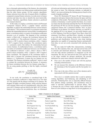
Table 1 summarises each of the papers discussed in this
section considering category, classification methods used,
selected features, traffic (simulated or real), and year.
Paper Category DL Method Features Traffic Year
Falahatraftar[14] Congestion Control Regression Neural
Network
No. of vehicles, data rate, transmission
power, and bandwidth
OMNeT++ 2022
Demir [15] Congestion Control SVM RTT, RTO Cooja Network 2020
Sander[10] Congestion Control RNN+LSTM Packet arrival Mininet 2019
Xiao[7] Congestion Control Deep Reinforcement
Learning
Size of congestion window, RTT,
inter-arrival time of ACK
NS-3 2019
Najm[17] Congestion Control Decision tree CWND, Throughput, Queue Size,
Packet Loss
NS-3 2019
Doshi[11] DDoS attacks KNN,LSVM,DT,RF Packet header fields, flow information
over very short time windows
Consumer IoT
device network
2018
Sivanathan[12] IoT device
classification
Multi-stage machine
learning
Activity cycles, port numbers,
signaling patterns, and cipher suites
Real network
Traffic
2018
Lopez [13] Protocol-wise
traffic Classification
CNN+RNN Source port, destination port, payload
size, TCP window size, inter-arrival
time, and flow direction
Real data from
RedIRIS
2017
Table 1. State-of-the-art comparison
3. PROBLEM STATEMENT AND METHODOLOGY
Real-time traffic volume prediction plays a vital role
in proactive network traffic management. Many forecasting
models have been proposed to address this issue.26-27
However,
most of them suffer from the inability to fully utilize the rich
informationintrafficdatatogenerateefficientandaccuratetraffic
predictions from longer-term data (e.g., seven-day predictions
at a five-minute interval). The accuracy of prediction of traffic
flow depends on the availability of historical data along with a
reliable technique that can filter the intrinsic properties from the
dataset to precisely forecast future flows. Let, the IoT network
has the N number of IoT devices. R is a volume of real network
traffic at a time t at the gateway node represented by (R, t). R
at (t + n) is the volume of real network traffic for the next time
point t + n and is represented by (R, t + n). The traffic volume
prediction problem at time t is defined to find the predictor of
(R, t) via a sequence of historical or training traffic datasets
(Rt−1
, Rt−2
, Rt−3...,
Rt−T
). The key problem here is to develop or
apply a model that defines the inherent relationships between
the historical or training dataset and prediction of network
traffic so that the network system can be able to accurately
predict the traffic volume to control congestion.
3.1 METHODOLOGY
This section describes a proposed methodology for
predicting congestion in the IoT network as shown in Fig. 1.
The big issue in our work was the lack of a publicly available
labeled dataset of congestion scenarios for IoT networks. To
the best of our search, we could not find any such dataset to
solve the problem statement.
Therefore, as the first step, we set up our own IoT home
testbed, as shown in Fig. 2. There are two main reasons to
design a home IoT testbed (i) to capture network traces from
real-world IoT devices and (b) to develop a realistic smart
environment for evaluating the proposed approach. Figure 2
describes the proposed IoT testbed environment. In our IoT
network setup, we use the computer (Ubuntu installed) having
two network interface cards (NIC1, NIC2). NIC 1 serves as a
gateway and connects to the Internet, while NIC 2 uses an L2
(S.No 13) switch to connect to the rest of the network. We use a
4G TP-Link MR6400 (S.No 14) router running CoAP, DHCP,
NAT, and DNS forwarding. The public Internet is accessible
through this TP-Link. An Unifi Access Point (S.No 12) is
connected to the L2 switch. The devices that are connected
with Ubiquiti Access Points are as follows.
• General-purpose hubs (3, 7)
• Several consumer electronics (4, 5, 6),
• Two smart plugs (9) can accommodate extra offline
devices
• Environmental devices (1, 8, 2).
With the L2 switch, the device-specific hubs (10 and 11)
are linked. These hubs control the devices that are plugged
into them. L2 switch routes all incoming and outgoing traffic,](https://image.slidesharecdn.com/congestionpredictionininternetofthingsnetworkusingtemporalconvolutional-1-231214082144-1c4ca211/85/Congestion-Prediction-in-Internet-of-Things-Network-using-Temporal-Convolutional-1-pdf-4-320.jpg)


More Related Content
Similar to Congestion Prediction in Internet of Things Network using Temporal Convolutional-1.pdf (20)
Recently uploaded (20)


![[HIFLUX] High Pressure Tube Support Catalog 2025](https://cdn.slidesharecdn.com/ss_thumbnails/tubesupporten-250529073613-16c22974-thumbnail.jpg?width=560&fit=bounds)

Congestion Prediction in Internet of Things Network using Temporal Convolutional-1.pdf
- 1. 810 Congestion Prediction in Internet of Things Network using Temporal Convolutional Network: A Centralized Approach Vinesh Kumar Jain,# Arka Prokash Mazumdar$ and Mahesh Chandra Govil% # Engineering College Ajmer, Ajmer, Rajasthan - 305 025, India $ Malaviya National Institute of Technology, Jaipur, Rajasthan - 302 017, India % National Institute of Technology, Sikkim - 737 139, India E-mail: [email protected] Abstract The unprecedented ballooning of network traffic flow, specifically the Internet of Things (IoT) network traffic, has big stress of congestion on today’s Internet. Non-recurring network traffic flow may be caused by temporary disruptions, such as packet drop, poor quality of services, delay, etc. Hence, network traffic flow estimation is important in IoT networks to predict congestion. As the data in IoT networks is collected from a large number of diversified devices with unlike formats of data and manifest complex correlations, the generated data is heterogeneous and nonlinear. Conventional machine learning approaches are unable to deal with nonlinear datasets and suffer from the misclassification of real network traffic due to overfitting. Therefore, it also becomes hard for conventional machine learning tools like shallow neural networks to predict congestion accurately. The accuracy of congestion prediction algorithms plays an important role in controlling congestion by regulating the send rate of the source. Various deep learning methods, such as LSTM, CNN, and GRU, are considered in designing network traffic flow predictors, which have shown promising results. This work proposes a novel congestion predictor for IoT that uses TCN. Furthermore, we use the Taguchi method to optimize the TCN model which reduces the number of experiment runs. We compare TCN with the other four deep learning-based models concerning Mean Absolute Error (MAE) and Mean Relative Error (MRE). The experimental results show that the TCN-based deep learning framework achieves improved performance with 95.52% accuracy in predicting network congestion. Further, we design the Home IoT network testbed to capture the real network traffic flows as no standard dataset is available. Keywords: IoT; TCN; Congestion; Taguchi; Prediction; Classification Received : 31 August 2021, Revised : 26 October 2022 Accepted : 14 November 2022, Online published : 6 December 2022 1. Introduction The use of Internet-connected smart devices, otherwise called the Internet of Things (IoT), is increasing rapidly in our homes, offices, smart cities, and many other places. These IoT devices are resource constrained, and a continuous rise in the volume of network traffic may lead to network congestion.1 A high traffic volume in IoT networks leads to extra communication delay, low network throughput, and waste of computing resources and bandwidth.2 These reasons ultimately become the cause of congestion. Diagnosing network congestion and building a framework that can classify and predict it is one of the most important issues3 as it affects the decision of the routing path process and optimal bandwidth utilization. Therefore, for effective communication in the network, it is essential to classify and predict congestion and take appropriate preventive measures accordingly. Hence, research for the classification and prediction of congestion in the network, especially for IoT networks, is extremely important. Typically, state-of-the-art congestion prediction in IoT networks relies on conventional techniques4–6 as used in Wireless Sensor Networks (WSN). These research works are focused only on the computing revolution, including the usage of high-end computers and advanced algorithms for managing traffic and performing flow prediction. Few efforts have been made to forecast short-term traffic flow, including simulation techniques,7 mathematical models, statistical approaches, and regression techniques. The data created by IoT networks are heterogeneous since it is gathered from numerous diverse devices with different data formats and complex correlations. As a result, it also becomes very challenging for traditional machine learning technologies, such as shallow neural networks, to effectively forecast congestion. Machine learning methods attain poor performance when dealing with high dimensional state spaces in congestion control problems, and their performance does not improve with increasing data. In particular, it is expensive to measure the traffic volume when there is high traffic on the IoT network. The traditional feature selection techniques of machine learning mainly consider the port and payload as features. Reusability and unfixed assignment of port numbers make it less effective to choose a port as a dominant feature in traffic classification. In contrast, payload as a feature fails due to encrypted traffic packet inspection. The problem in IoT Defence Science Journal, Vol. 72, No. 6, November 2022, pp. 810-823, DOI : 10.14429/dsj.72.17447 © 2022, DESIDOC
- 2. Jain, et al.: Congestion Prediction in Internet of Things Network using Temporal Convolutional Network 811 networks, like congestion prediction, is an adversarial problem due to random burst traffic and heterogeneity in devices and protocols. In such cases, machine learning techniques that learn from historical data can make the wrong prediction. Recently, statistical feature-based machine learning techniques have received attention, particularly in the field of wired and wireless networking.3,8 However, adopting machine learning as an invincible approach and using it for real-time IoT network traffic is not good. In contrast, deep learning is a centralized approach that uses basic information as direct input and automatically performs feature extraction. Deep learning eliminates the need for experts in a specific area by utilizing hierarchical feature extraction, which makes information distillation efficient, provides more abstract correlations in the data, and reduces the pre-processing effort. Deep learning algorithms can proficiently comprehend the features of a large amount of data. Parallel computation using graphics processing units (GPUs) allows deep learning to draw inferences in milliseconds. This allows for high-accuracy and timely network analysis and control, eliminating the run- time constraints of conventional mathematical approaches (e.g., convex optimization, game theory). The prediction of congestion in IoT networks has a temporal dependency. The temporal dependency means predicting congestion or a high traffic volume at a specific time instance is done based on past observations. Real-time prediction of network congestion requires continuous feeding and learning. The number of time slots may increase rapidly with time, which results in high computational complexity and also affects prediction accuracy. Recurrent Neural networks (RNN) and Long Short Term Memory (LSTM) are the most common deep learning methods to analyze time-series data. However, RNN models cannot directly calculate the long sequence of time points. In contrast, LSTM can process millions of time points, but it works sequentially, making it inefficient in generating timely responses. On the contrary, Temporal Convolutional Network (TCN), a deep learning-based model, has a parallel processing capability and training and forecasting time lower than LSTM.9 Therefore, in this work, we use the TCN model to predict congestion accurately. Our proposal also leverages the dropout technique of deep learning to cope with the overlearning problem. The proposed approach works for the real IoT network traffic for congestion prediction. In addition to state-of-the-art congestion control techniques in IoT networks, our proposal is a centralized approach toward congestion control that reduces the burden of end devices on congestion prediction. In summary, the following are the main contributions of our proposed approach. • We created a Home IoT network testbed and gathered the network traffic flows of various IoT applications because, as far as we are aware, there is no such labeled dataset of IoT network traffic available. • The traditional approaches use the brute force method to tune the hyperparameters and structure of deep learning models. Brute force approaches take a long time to train the model and are inefficient for achieving high prediction accuracy. The proposed approach uses a design of the experiment (DoE) based Taguchi method as a novel way to achieve the optimal structure of TCN to resolve this issue for IoT network traffic prediction. Compared with brute force approaches to tune and train the models, the Taguchi method decreases the number of trials required to tune hyperparameters and models, which results in the accuracy of forecasting results. • IoT networks have heterogeneous devices and irregular traffic flow. In such cases, when we train the model, it may be overfitted, and we do not have an accurate prediction as desired. We use the concept of regularization by applying the dropout layer to avoid overfitting. • We use a deep learning-based imputation technique to deal with missing values generated during data collection. This improves overall accuracy by converting incomplete data to complete data. • To the best of our knowledge, TCN has not previously been applied to congestion prediction and detection problems. Consequently, the work discussed in this paper is original by its very nature. The contour of the paper is as follows. Section 2 presents state-of-the-art work in the field of IoT network traffic classification and prediction. Section 3 formulates IoT network traffic problems and emphasizes the necessity of deep networks for IoT network traffic classification and prediction along with the proposed methodology. Section 4 represents the structure of TCN and hyper-parameter tuning by the Taguchi Method. In Section 5, empirical results of deep learning models about the accuracy of prediction and the role of activation functions in enhancing real-time prediction accuracy are presented. The conclusion and future scope of this work are presented in Section 6. 2. RELATED WORK Most of state-of-the-art in the area of IoT networks is related to IoT congestion control,7,10 classification of network attacks based on the traffic,11 IoT device classification,12 and traffic classification13 incorporating machine learning and deep learning. In this section, we introduce and analyze state-of-the- art. Heterogeneous vehicular networks may experience congestion due to increased resource demands for data transmission as a result of the rise in intelligent vehicle adoption and the popularity of various safety and comfort applications. Safety applications, including emergency braking systems, traffic danger alerts, and collision avoidance signals, require low latency and high bandwidth. Unfortunately, congestion often reduces network performance and customer pleasure (QoS) by reducing the quality of service. Reduced QoS is also a result of inadequate mobility models, routing protocols, and communication mediums. Falahatraftar, et al.14 proposed a congestion prediction and avoidance approach named Intelligent Congestion Avoidance Mechanism (ICAM) based on the Generalized Regression Neural Network (GRNN). The authors compared the proposed GRNN congestion prediction
- 3. Def. SCI. J., Vol. 72, No. 6, november 2022 812 model with other widely used models, including Multiple Linear Regression (MLR), Support Vector Machine (SVM) for Regression, Decision Tree Regression (DTR), and Multi-layer Perceptron for Regression (MLPR). The proposed GRNN congestion prediction model performs than other models in terms of accuracy, dependability, and stability, according to numerical data. In addition, simulation findings demonstrate a significant network performance gain in terms of packet delivery ratio, average latency, and packet loss ratio when compared to conventional congestion control strategies. Demir, et.al15 proposed mlCoCoA, a machine learning- based enhancement in CoCoA [16], the advanced variant of the Constrained Application Protocol (CoAP). CoCoA is used to control congestion by estimating the Re-transmission Timeout (RTO) values, as shown in equation 1. RTT is the round trip time, and RTTVAR gives the difference between the successive RTT and current RTT measurements. Here, x is a variable that denotesthestrongandweakRTT.StrongRTTiscalculatedwhen an acknowledgment is received without any retransmission. Weak RTT is calculated when an acknowledgment is received after the number of retransmission. Here α, β, λ, and K are the constants, and their values are defined statically. x x x x new| RTTVAR (1 )*RTTVAR *| RTT RTT − = −β +β − x x x new| RTT (1 )*RTT *RTT − = − α + α x x x x RTO SRTT k *RTTVAR = + overall x overall RTO *RTO (1 )*RTO = λ + − λ (1) TheapproachmlCoCoAclaimsthatthedynamicprediction of the values of these constants using machine learning can increase the network throughput of the IoT network. The authors performed the set of experiments by creating the CoCoA network for collecting the ground truthα, β, λ, and K. The SVM predicts the values of these constants. The precise estimation of RTO provided by the accurate prediction of these values reduces unnecessary retransmission. Sander,10 et al. proposed DeePCCI to identify congestion based on packet arrival time (passive entity) in traffic flow. Being based on the usage of passive knowledge, it works on encrypted transport headers also. DeePCCI architecture is the combination of CNN and LSTM, which are parts of a Deep Neural Network (DNN).The only feature taken is packet arrival time, whose histogram bins of size 1 ms are generated and then fed into the DNN and extracted through 2D VGGNet-13.18 The authors used the single host, multiple hosts, and mininet- based network testbeds by using the standard Linux 4.18 Kernel to generate the network traffic. The authors evaluated the performance on various vantage points after and before the bottleneck giving the final accuracy of the chosen network in BBR, CUBIC, RENO, CUBIC-p, and RENO-p. The authors19 analyzed the performance of DeepCCI and showed that it has limited performance because the training is done using testbed- generated data that lacks the Internet’s inherent noise. Further, they observe that DeepCCI needs to be re-trained for different kernels to capture behavioral differences appropriately. Xiao,7 et al.proposed TCP-Drinc for smartly controlling congestion for the TCP variants. The authors use Deep Reinforcement Learning20 which learns from experience. Congestion is controlled by adjusting the window size. The authorsusedthedeepconvolutionsneuralnetworkandextracted stable features from abundant but noisy data measurements. TCP-Drinc is compared with the various versions of TCP, i.e., TCP-New Reno,21 TCPCubic,22 TCP-Hybla,23 TCP-Vegas,24 and TCP-Illinois.25 TCP-Drinc yields maximum throughput and the second lowest Round Trip Time for the entire period of propagation delay. TCP-Drinc has a higher round trip time than TCP-Vegas. Najm,17 et al.proposed a novel machine learning-based model built upon a decision tree algorithm for predicting congestion in 5G IoT networks. The authors determine the optimal congestion window using specific network conditions, including high throughput, high congestion window, large queue size, and low loss. The authors applied C4.5, RepTree, and Random Tree-based decision tree approaches along with clustering and stacking approaches. The results show that the C4.5decisiontreealgorithmhasthebestperformancecompared to other machine learning algorithms; The authors present a tree-based graph that suggests the optimal path through which congestion can be controlled. The authors compared their model with the original Stream Control Transmission Protocol (SCTP) and claimed a 14.5 % improvement in performance. Doshi,11 et al.worked on detecting distributed denial of service (DDoS) attacks using well-known machine learning algorithms in the IoT network. A large number of Botnets like Mirai leveraged vulnerable IoT devices for performing DDoS attacks in IoT networks. The network includes IoT devices such as home gateway routers and other middleboxes for keeping track of traffic flow between IoT devices on the local network and the rest of the Internet. Binary classification is applied to separate the data for both DDoS attacks as 0 and 1. Data is collected from the devices, such as home cameras and Bluetooth devices connected to blood pressure monitors, all connected to the router via Raspberry Pi. Non-IoT traffic is filtered out from the pcap files. Sivanathan,12 et al. proposed a robust approach for classifying IoT devices using traffic characteristics that are acquired at the network level. A setup with 28 IoT devices and a few non-IoT devices was created to validate the proposed approach. OpenWrt was used to monitor the traffic flow for 26 weeks.26 Each of the devices showed some pattern for different network characteristics. Among all the features, nine features were selected to perform the classification: a bag of a port number, a bag of domain names, a bag of cipher suites, flow volume, DNS interval, flow duration, sleep time, flow rate, and NTP interval. All the data with these features were fed into a two-stage machine learning model, which predicted the confidence for a particular type of IoT device. The first stage, called Stage 0, implements the Naive Bayes Multinomial Classifier independently for features, viz., a bag of the port number, bag of domain names, and bag of cipher suites. Each of these features returned moderate accuracy for different devices. Then the output of all these three classifiers is fed into the second stage, i.e., Stage 1. In Stage 1, the outputs from the Naive Bayes Multinomial Classifier and the remaining six features were fed into the Random Forest Classifier,
- 4. Jain, et al.: Congestion Prediction in Internet of Things Network using Temporal Convolutional Network 813 which provided the required confidence for each input. This confidence is then mapped to the IoT device’s classes, and the authors obtain the desired classification of IoT devices. Lopez, et al.13 proposed a network traffic classifier (NTC) to predict the network services among different communication protocols. The proposed network traffic classifier considers the flow-based features, e.g., source and destination ports and bytes transmitted per packet. The authors used the different deep learning models and their combinations (RNN, CNN, and CNN+RNN) to infer the network services. NTC uses the RedIRIS dataset consisting of 266,160 network flows from 108 services to validate the approach. The results show that the combination of CNN+RNN has the best accuracy in terms of F1 score, precision, and recall. Table 1 summarises each of the papers discussed in this section considering category, classification methods used, selected features, traffic (simulated or real), and year. Paper Category DL Method Features Traffic Year Falahatraftar[14] Congestion Control Regression Neural Network No. of vehicles, data rate, transmission power, and bandwidth OMNeT++ 2022 Demir [15] Congestion Control SVM RTT, RTO Cooja Network 2020 Sander[10] Congestion Control RNN+LSTM Packet arrival Mininet 2019 Xiao[7] Congestion Control Deep Reinforcement Learning Size of congestion window, RTT, inter-arrival time of ACK NS-3 2019 Najm[17] Congestion Control Decision tree CWND, Throughput, Queue Size, Packet Loss NS-3 2019 Doshi[11] DDoS attacks KNN,LSVM,DT,RF Packet header fields, flow information over very short time windows Consumer IoT device network 2018 Sivanathan[12] IoT device classification Multi-stage machine learning Activity cycles, port numbers, signaling patterns, and cipher suites Real network Traffic 2018 Lopez [13] Protocol-wise traffic Classification CNN+RNN Source port, destination port, payload size, TCP window size, inter-arrival time, and flow direction Real data from RedIRIS 2017 Table 1. State-of-the-art comparison 3. PROBLEM STATEMENT AND METHODOLOGY Real-time traffic volume prediction plays a vital role in proactive network traffic management. Many forecasting models have been proposed to address this issue.26-27 However, most of them suffer from the inability to fully utilize the rich informationintrafficdatatogenerateefficientandaccuratetraffic predictions from longer-term data (e.g., seven-day predictions at a five-minute interval). The accuracy of prediction of traffic flow depends on the availability of historical data along with a reliable technique that can filter the intrinsic properties from the dataset to precisely forecast future flows. Let, the IoT network has the N number of IoT devices. R is a volume of real network traffic at a time t at the gateway node represented by (R, t). R at (t + n) is the volume of real network traffic for the next time point t + n and is represented by (R, t + n). The traffic volume prediction problem at time t is defined to find the predictor of (R, t) via a sequence of historical or training traffic datasets (Rt−1 , Rt−2 , Rt−3..., Rt−T ). The key problem here is to develop or apply a model that defines the inherent relationships between the historical or training dataset and prediction of network traffic so that the network system can be able to accurately predict the traffic volume to control congestion. 3.1 METHODOLOGY This section describes a proposed methodology for predicting congestion in the IoT network as shown in Fig. 1. The big issue in our work was the lack of a publicly available labeled dataset of congestion scenarios for IoT networks. To the best of our search, we could not find any such dataset to solve the problem statement. Therefore, as the first step, we set up our own IoT home testbed, as shown in Fig. 2. There are two main reasons to design a home IoT testbed (i) to capture network traces from real-world IoT devices and (b) to develop a realistic smart environment for evaluating the proposed approach. Figure 2 describes the proposed IoT testbed environment. In our IoT network setup, we use the computer (Ubuntu installed) having two network interface cards (NIC1, NIC2). NIC 1 serves as a gateway and connects to the Internet, while NIC 2 uses an L2 (S.No 13) switch to connect to the rest of the network. We use a 4G TP-Link MR6400 (S.No 14) router running CoAP, DHCP, NAT, and DNS forwarding. The public Internet is accessible through this TP-Link. An Unifi Access Point (S.No 12) is connected to the L2 switch. The devices that are connected with Ubiquiti Access Points are as follows. • General-purpose hubs (3, 7) • Several consumer electronics (4, 5, 6), • Two smart plugs (9) can accommodate extra offline devices • Environmental devices (1, 8, 2). With the L2 switch, the device-specific hubs (10 and 11) are linked. These hubs control the devices that are plugged into them. L2 switch routes all incoming and outgoing traffic,
- 5. Def. SCI. J., Vol. 72, No. 6, november 2022 814 which mirrors all testbed traffic on the switch port attached to the Ubuntu PC. On the Ubuntu PC, we set up the following packages: Wireshark (for traffic capture), block-mount package kmod-USB-core (for mounting external USB base memory), and package kmod-USB-storage (for storing the network traffic traces on USB storage). A bash script is run to automate the data collecting and storage. This execution of script records pcap files on an external USB storage device that is connected to the PC. We collected the network traffic traces after the testbed has been set up. We introduced a burst into the network to generate congestion because the goal is to predict network congestion. We collect the network traces in the form of pcap files using Wireshark. This network data contains traffic traces and session logs of different devices at network layers as per the requirement of applications. For example, congestion detection problem in IoT network often needs datasets of packet-level traces labeled along with corresponding classes. Wireshark’s filters are used to segregate congestion states from the normal traffic states. We filtered congestion traffic with the help of Bad TCP, ICMP errors, Retransmission, and Duplicate ACK filters and stored this traffic in the pcap file named “congestion.” The rest of the traces of normal traffic are stored in another pcap file named “normal.” Figure 1. Methodology. Figure 2. IoT home testbed for data collection. We use CICFlowmeter to convert these two pcap files to comma-separated values (CSV) files. CICFlowMeter is a network traffic flow generator and analyzer that produce 83 network traffic features from the pcap files. Hence, there are 83 columns in the CSV file. CICFlowMeter provides bidirectional flows from source to destination and destination to a source with duration, number of packets, number of bytes, length of packets, etc. These features are calculable separately in both directions. These columns contain low-level features (Flow ID, Source IP, Destination IP, Source port, Destination port, and protocol) and other high-level features. We added class labels (Congestion, No Congestion) in the last column of both CSVs. WeperformtheExploratoryDataAnalysis(EDA)29 fordata pre-processing. EDAhelps to find various information about the data, such as missing values, normalization, mean categorical data, median, distribution of data, and correlations. We carry out the EDA using the Profiling tool. After removing all the noise, inconsistency, and missing values, we obtain a complete and accurate dataset. Now, we start looking for relations among various features of the data. The feature selection process can be done manually or using some mathematical or algorithmic techniques. In the case of manual feature selection, one must
- 6. Jain, et al.: Congestion Prediction in Internet of Things Network using Temporal Convolutional Network 815 have a thorough understanding of the features, the relationship between them, and how one feature group would perform better than the other feature groups. On the contrary, algorithmic feature selection lowers the role of manual efforts. In addition, compared to manual feature selection, it avoids errors in feature selection and takes less time to identify the most trustworthy features. Therefore, algorithmic feature selection is preferred over manual selection. In this study, we employ a correlation matrix and Principal Component Analysis (PCA), a popular feature selection algorithm, to analyse the relationship between various features inthedataset.30 Thecorrelationmatrixisasymmetricmatrixthat defines the relationship between various fields. In mathematical terms, a correlation matrix is a matrix of correlation coefficients between a set of variables. The diagonal of the correlation matrix is filled with 1s because the correlation between the same variables is 1. The coefficient is between -1 and 1, where 1 shows a 100 % positive linear correlation, while -1 depicts a 100 % negative linear correlation. The correlation matrix is a symmetric matrix that defines the relationship between various features. In mathematical terms, a correlation matrix is a matrix of correlation coefficients between a set of features. The coefficient is between -1 and 1, where 1 shows a 100 % positive linear correlation, while -1 depicts a 100 % negative linear correlation. The diagonal of the correlation matrix is filled with 1s because the correlation between the identical features is 1. Furthermore, 0 means the two features are not correlated. The Pearson correlation coefficient31 metric is used to evaluate the correlation between the features. It measures the linear correlation between the two features using Eqn. 2. We are using pandas profiling to find the highly correlated features. ( ) ( ) ( ) ( ) Cov X,Y X,Y = Var X Var Y ρ (2) In our work, the correlation is considered high if the Pearson correlation coefficient is larger than 0.9 or less than -0.9. We started with the dataset consisting of 83 features. We dropped 30 highly correlated features, along with the features with constant values such as 0 simultaneously. After this, there were still 53 features and one field for the label. All 53 of these features were useless for our prediction, thus, we eliminated all irrelevant information and retained only those necessary for the system to learn. The following columns, as indicated in Table 2, are removed during the learning process based on the results of pandas profiling. Flows ID, Destination IP, Source IP, and Timestamp are categorical and sparse features that increase the space and time complexity of the models. The historical time series data, which contains a timestamp, is used to predict the future. As a result, we retain only the timestamp and drop the Flow ID, Destination IP, and Source IP. We use one-hot encoding32 to transform this categorical feature into a numerical attribute. Now, we have 50 features in our dataset. For feature selection, we used PCA. On applying PCA to our dataset, we got useful features such as Flow Duration, Fwd Pkt Len Mean, Flow Pkts/s, Bwd IAT minimum, Fwd Pkts/s, and Bwd Pkts/s. Initially, we decided to go with these seven features along with a timestamp for prediction and classification. However, since deep learning approaches are capable of recognizing features automatically from data, we are not overly concerned with selecting more features. We also study IoT traffic flow characteristics, including flow size, flow duration, flow rate, and inter-arrival time (∆T) in forward and backward directions. These characteristics will also help advance prediction of congestion on the nth timestamp. We also use inter-arrival time (∆T) and flow rate as the target variable for advance prediction. We provide definitions for some terms related to network traffic flow. • Flow size is the number of bytes sent with the payload, including retransmissions. • We can measure flow duration as the difference between the timestamp of the first packet and the last packet in a flow. • Flow rate is the ratio of flow size to flow duration and is represented with flow packets/second Flow size is a valuable statistic that is used to optimize routing algorithms, load balancing, and scheduling in IoT networks. Predicting flow size is especially difficult because flow patterns change constantly, and calculations must be made in real-time (milliseconds) to prevent delays. This is because the size of flows varies greatly (from small mice flows of a few kilobytes to large flows of several gigabytes), as Active Max Subflow Bwd Packets Bwd IAT Max Active Min Idle Min Fwd Bulk Rate Avg Bwd PSH Flags Packet Length Min Bwd URG Flags Idle Max Fwd IAT Total Bwd Bytes/Bulk Avg Bwd Segment Size Avg Fwd Packet/Bulk Avg Fwd URG Flag URG Flag Count Active Mean ECE Flag Count Fwd Bytes/Bulk Avg ACK Flag Count Fwd Packets/s Bwd Packet Length Std Subflow Bwd Bytes Fwd IAT Std Bwd IAT Std Fwd IAT Mean Active Std Packet Length Mean Fwd IAT Max Fwd Segment Size Avg Table 2. Features to be dropped
- 7. Def. SCI. J., Vol. 72, No. 6, november 2022 816 well as the length of time they inhabit a route (milliseconds to hours). Since large flows hold the route for a longer time (flow duration) than small flows, there’s a chance that the number of active flows will become unbalanced due to a concentration of large flows in the routing path. The quantity of available data determines the selection of a deep learning model. The data patterns may or may not be consistent due to the irregular traffic flow. The chances of the overfitting of the model may be high when we collect the data from these networks. The selection of the model in these types of cases is crucial. For example, accurate congestion prediction can suggest how much the sending rate of a node in the IoT network should be controlled. The deep learning algorithms may reduce the chances of overfitting. Motivated by the excellent performance of deep learning techniques in images and natural language processing, we select TCN, LSTM, Gated recurrent unit (GRU), Stacked autoencoder (SAE), and CNN-LSTM models for the solution of proposed IoT network traffic classification and prediction approach.33 These techniques have the capability of automatically learning the features. The model validation verifies the overall accuracy of the model in terms of overfitting and underfitting. This verification of accuracy helps to optimize the model by increasing the volume of data and reducing the complexity of the model when data overfits. Analysis of wrongly classified samples helps to find the reasons for errors and check the suitability of the model and features. The processed dataset is divided into three parts, i.e., training (60 %), validation (20 %), and testing (20 %). We train different models with training data using various combinations and different values of hyper- parameters. Further, re-training is done on the different training and validation dataset combinations using the same set of hyper-parameters, and the accuracy is calculated for testing the dataset. We observe overfitting initially, as the training score is high, but the validation score is low. This score shows that the model has adapted well to the specific training dataset. However, the trial-and-run process to train a model is time- consuming. Therefore, we have used the Taguchi method to optimize the hyper-parameter and train the model. This method reduces the number of trials to optimize hyper-parameters. 4. MODEL CONSTRUCTION AND PARAMETER TUNING In this section, we represent the basic architecture for convolution sequence forecasting and hyper-parameter tuning which is an integral part of the neural network. The series of IoT network traffic flow of length T with the input sequence {p1 ,p2 ,.....pT } is utilized for predicting the output sequence of traffic flow {q1 ,q2 ,.....qT }. Here, observed data {p1 ,p2 ,.....pt } is the input to the model for the forecast of the output t q at the time t. Equation 3 defines the function t t f:P Q → prediction of the traffic flow. { } ( ) { } 1 2 T 1 2 T q ,q , q = f p ,p , p …… …… (3) Here, the function f must hold the condition that the t q depends only on historical data { } 1 2 t 1 p ,p ,......p − rather than { } t+11 t+2 T p ,p ,......p . Equation 4 defines the function to forecast network traffic flow t q at time t as follows. ( ) { } t 1 2 T q = f p ,p , p …… (4) 4.1 Temporal Convolutional Network TCN34 isthevariationofCNNforsequencemodelingtasks. TCN is designed by combining the features of the RNN and CNN. TCN uses casual convolutions and dilated convolutions. The casual convolution is used for temporal data and ensures that the model will not violate the sequence in which the data is modeled. The prediction relies only on the historical data, not on future observations. TCN model inherits the property of 1-D fully convolution of generating the same length output as the input, and subsequent layers maintain the same length by adding zero padding to avoid information leakage. The accurate prediction of the traffic flow requires a large history and a very deep network. This makes the network structure of the model complicated and computationally intensive. The integration of dilated convolutions and residual layers with TCN solves this issue. Dilated convolutions, in particular, allow for an exponentially large receptive field to cover large history. Equation 534 shows the dilated convolution operation F on elements of the sequence s for the given 1-D sequence input n p R ∈ and a filter { } f: 0.k 1 R − → . ( ) ( )( ) ( ) k 1 f s d.i i=0 F s = p d s = f i .p − − ∗ ∑ (5) Here, d represents the dilation factor; i stand for past direction, k denotes the size of filter f, and i d s . − maintain the history. The value of dilation factor d = 1 for dilated convolution in equation 5 works as the standard convolution. The exponential adjustment to d increases the receptive field size that covers the large history with the depth of the deep learning network. This represents the large range of inputs by leading the output at the top level. Filter size k is used to increase the receptive field of TCN. However, this approach increases parameter count and execution time, resulting in slow and overfitting of the model. The residual connection is the next important part of TCN that includes a branch towards a series of transformations F, whose outputs q are connected to the input p of the block. Figure 3 shows the diagram of the residual block. This block contains two weight layers along with the Rectified Linear Unit (ReLU) activation function. Moreover, regularization is achieved by connecting a spatial dropout layer after the last weight layer. Here, Eqn. (6) defines the residual block mathematically. ( ) i q = F p,W + p (6) Here, q is the output layer. The function F(p,Wi ) shows the residual mapping to be learned, where Wi denotes the weights of ith layer. The function for two layers of TCN is represented as 2 1 F W (W p) e, = σ + in which σ and e represent ReLU and
- 8. Jain, et al.: Congestion Prediction in Internet of Things Network using Temporal Convolutional Network 817 bias, respectively. To predict and detect network congestion in a home IoT network, we use TCN architecture. TCN architecture is made up of a collection of blocks; each block contains a set of N number of convolutional layers. Layers are made up of dilated convolutions with a dilation factor d and a nonlinear activation function f(.) associated with it. The convolution outcome is integrated with the layer’s input by using a residual relation in each dilated convolution. ( ) ( ) t 2 i i=0 1 L = q F i t − ∑ (11) Here, Fig. 4 shows TCN model architecture that uses 19 convolutional layers and a fully connected layer. Convolutional layers are shown in a rectangular area with a grey background. In Figure 4, the grey rectangles in the shaded rectangle show that the result of convolutional layer 1 is applied as the input of convolution layer 3 by using the residual structure directly. The kernel size 10 and filter size 24 are used for all the convolutional layers. TCN model is trained with the processed training data. The final TCN with the enhanced configuration is transmitted to the central server depending on the feedback of the historical traffic flow data sequence and is used for forecasting packet flows/sec in the next 30 minutes in the network given the past traffic flow in the dataset. Figure 3. TCN residual block. Equation (7) describes the activation function for the ith layer and jth block ( ) F i.j w T S R × ∈ (7) Here, we can note that every layer has the same number of filter Fw . We define the output of the dilated convolution at time t as j,l t S and the convolution result after the residual connection l j, S as shown in Eqn (8). ( ) j,l 1 j,l 1 2 j,l 1 t t d t S = f W S + W S + b − − − j,l j,l j,l t t S = S + VS + e (8) Here, 1 W and 2 W denote the weight parameters. F F w w V R × ∈ is the set of weights and Fw e R ∈ represents the biases for the residual, respectively. The output of each block is summed by a group of skip connections with T F 0 w t Z R × ∈ satisfying Eqn. (9) B 0 j,L t t j=1 Z = ReLU S ∑ (9) The latent result 1 t Z is ( ) 0 r t r ReLU V Z + e for the weight matrix Vr and the bias er . We can represent the forecasting through Eqn. (10) ( ) ( ) 1 t t q = softmax UZ + c (10) Here, U is the weight matrix C Fw U R × ∈ and bias C c R . ∈ Equation 11 shows the objective function of the model. We aim to minimize the value of L by keeping the training of the data. At time t, qt gives the forecasting result. The initial traffic flow at time t is represented by F(t). Parameters are configured as follows at the time of training of the TCN model; batch size 128, number of epochs 30, dropout as 0.5, and initial learning rate as 0.002. We use the stochastic gradient descent technique to decrease the learning rate at the time of training. Figure 4 TCN architecture. 4.2 Hyper-parameter Tuning Building a deep learning model for network traffic flow prediction requires the best combination of neural network parameters such as kernel size, number of filters, dilations list, count of residual block stacks, etc. Traditionally, a trial- and-error approach is used to find out the best combinations of these hyper parameters. However, it is inefficient in yielding high precision and time-consuming because it requires a huge number of trials. This prompted us to look for more coherent alternatives to the traditional trial-and-error approach. Instead, Zhao, et al.34 used the Taguchi approach to predict short-term traffic movement accurately or identify congestion sites for intelligent transportation systems (ITS) in smart cities. We believe that the problem of road traffic congestion is similar
- 9. Def. SCI. J., Vol. 72, No. 6, november 2022 818 to the problem of network congestion, so we also incorporate the Taguchi method to determine the optimized values of the hyper-parameters of the deep learning model for IoT network congestion prediction. We have executed a small series of experiments to see if we could improve the structure of deep learning models that were trained by the training dataset. The trialrunresultsshowthedisparitybetweentheexpectedandreal performance. The findings of the trial run help determine the most suitable hyper-parameter values for efficient performance metrics. The topology of the deep learning-based TCN model is then determined. The Taguchi approach is divided into three parts: (i) Design factors identification, (ii) Trial design and performance metrics, and (iii) Optimization of the model structure and performance analysis. The first step of the Taguchi method is identifying the design factors and their corresponding levels. These design factors greatly influence the topology determination of the deep learning models. The number of filters used in deep learning models is considered the first design factor. The state- of-the-art shows that the most frequent number of filters used is 6, 12, and 24. We follow the same practice and use the 6, 12, and 24 filters at Levels 1, 2, and 3, respectively. The size of the kernel is the second design factor. We use the 10, 15, and 20 kernel sizes at each layer of the deep learning model for Levels 1, 2, and 3, respectively. The list of dilation is the third design factor. The list of the dilation gives the size of the deep learning model. We set the list A {20 , 21 , 22 , 23 , 24 }, list B {20 , 21 , 22 , 23 , ..., 29 }, and list C as {1, 2, 3, ..., 9} for Levels 1, 2, and 3, respectively. The number of stacks of residual blocks is the fourth design factor. The state-of-the-art suggests the use of 2 to 9 stacks of residual blocks. We set the numbers 2, 6, and 9 stacks of residual blocks for Levels 1, 2, and 3, respectively. We assess the performance of deep learning models for congestion prediction using Mean Absolute Error (MAE) in Eqn. (12) and Mean Relative Error (MRE) in Eqn. (13). These performance metrics show the absolute and mean difference between the actual network flow and the one predicted by the model, respectively. ( ) n n i i i=0 i=0 1 MAE = f f n − ∑∑ (12) ( ) n i i i=o i f f 1 MRE = n f − ∑ (13) Here, i f and i f are actual and predicted traffic flow duration respectively. Here, n shows the number of forecast points. Lower MAE and MRE are the indicators of less difference between the actual flow and predicted flow, which shows better accuracy of prediction. As we have three levels and four design factors, the full factorial design requires a total of 81 trials. As prediction problem requires a large amount of historical data, full factorial design may be time-consuming. Therefore, we use fractional factorial designs. As with the consideration of four design factors along with three levels for each, we build an orthogonal arrayA16 (34 )forthetrialdesign.Wehaveoptimizedthestructure of the deep learning model by executing the combination of design factors along with their levels in 16 trials. Every row of the orthogonal array A16 (34 ) related to the main trial develops a deep learning model using a training dataset of the home IoT testbed. Table 3 shows the results of the 16 main trials for the seven days (March 1-7, 2021), along with the average result of the testing dataset. The accuracy of deep learning models is evaluated by the collected data of the Home IoT testbed over seven days with 16 main trials. The results in Table 3 depict Main Trials Level Day MAE MRE Average Result of 5 Days i ii iii iv MAE Rank MRE Rank 1 1 1 1 1 1st 65.783 0.899 59.532 16 0.447 16 3rd 17.12 0.335 5th 44.082 0.125 2 1 2 2 2 1st 20.991 0.255 21.732 7 0.1 5 3rd 0.128 0.004 5th 3.682 0.048 3 1 3 3 3 1st 23.323 0.286 24.258 10 0.11 8 3rd 1.387 0.029 5th 1.485 0.02 4 1 1 2 3 1st 293501 0.348 29.729 15 0.165 14 3rd 5.987 0.144 5th 8.229 0.108 5 1 1 3 1 1st 33.211 0.396 28.502 14 0.164 13 3rd 7.532 0.168 5th 2.621 0.033 Table 3. Orthogonal array A16 (34 ) and experimental outcomes
- 10. Jain, et al.: Congestion Prediction in Internet of Things Network using Temporal Convolutional Network 819 that the smallest MAE and MRE were obtained within the 16th trial with 24 numbers of filters, 2 numbers of stacks, a 15 kernel size, and the dilation with list A. In Table 3 top three trials are the 7th , 11th , and main trial 16th with list A setting of dilation. This concludes that the dilation with listAgives better accuracy than the other two lists. The main trials 1st , 4th , and 5th with the 6 filters and small kernel size perform poorly concerning MAE and MRE. This concludes that the performance of the deep learning models varies with the change in the combinations of the parameters. Every trial under the Taguchi method has orthogonal combinations. Hence, we can separately analyze the effect of individual design factors. The effect of every design factor at a specific level is determined by averaging the respective values in Table 3. In particular, the design factor i with Level 2 is in 6th , 7th , 8th , 9th , and 10th main trials, and we can find its average effects 23.9428 (MAE) and .121 (MRE). Table 3 shows the effects of all four design factors at all their corresponding three levels. The sensitivity (identification of true positive) of design factors is also determined using range analysis, which is defined as the difference between the highest and lowest performance values for each design factor. Table 4 displays the sensitivity data. We can find the order of the sensitivity by sorting the sensitivity values of four design factors from high to low, as i>ii>iv>iii in terms of MAE. The same concept applies to finding the order of the sensitivity in terms of MRE, and the order is as i>ii>iv>iii. These orders depict that the design factor i has the lower effect value of MAE and MRE; hence, it is considered the primary factor for the TCN forecasting model for better performance. Here, Tables 3 and 4 help to determine the optimized parameters of the TCN model for the IoT network traffic flow forecasting in the Home IoT testbed. These parameters are the design factors and i, ii, iii, and iv with values that exist at Level 2. TCN model 6 2 1 2 3 1st 23.334 0.275 20.936 4 0.104 7 3rd 1.876 0.044 5th 1.997 0.025 7 2 2 1 3 1st 16.305 0.201 20.326 3 0.093 3 3rd 1.249 0.027 5th 4.948 0.066 8 2 3 3 1 1st 34.147 0.397 28.396 11 0.146 11 3rd 1.771 0.038 5th 5.597 0.071 9 2 1 3 3 1st 29.527 0.342 28.5 12 0.162 12 3rd 4.212 0.095 5th 11.494 0.149 10 2 3 1 3 1st 19.635 0.229 21.556 5 0.1 5 3rd 1.916 0.044 5th 3.414 0.043 11 3 3 1 2 1st 13.916 0.165 20.029 2 0.092 2 3rd 2.838 0.064 5th 4.823 0.062 12 3 3 2 1 1st 39.97 0.466 28.755 13 0.197 15 3rd 9.729 0.218 5th 9.857 0.128 13 3 1 1 1 1st 1.488 0.018 21.785 6 0.094 4 3rd 5.184 0.116 5th 9.103 0.117 14 3 1 2 1 1st 22.765 0.255 24.963 9 0.115 9 3rd 0.436 0.015 5th 5.314 0.067 15 3 2 2 2 1st 33.132 0.387 24.834 8 0.143 10 3rd 4.307 0.094 5th 2.675 0.033 16 3 2 1 1 1st 20.191 0.234 16.156 1 0.081 1 3rd 0.306 0.008 5th 1.817 0.025
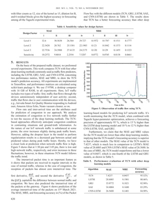
- 11. Def. SCI. J., Vol. 72, No. 6, november 2022 820 with filter counts as 12, size of the kernel as 15, dilation list B, and 6 residual blocks gives the highest accuracy in forecasting among all the Taguchi experimental trials. Design Factor MAE MRE i ii iii iv i ii iii iv Level 1 32.6 30.5638 26.564 29.727 0.1972 0.1787 0.1511 0.1777 Level 2 22.3428 20.762 25.1581 22.1983 0.121 0.1042 0.1373 0.1116 Level 3 22.7536 24.5988 27.4135 24.2175 0.120 0.129 0.1455 0.1223 Sensitivity 10.2572 9.8018 2.2554 7.5287 0.0772 0.0745 0.0138 0.0661 Table 4. Sensitivity values for design factors 5. RESULTS On the basis of the prepared traffic dataset, we preformed several experiments. This work compares TCN with four other deep-learning methods commonly used as traffic flow predictors, including the LSTM, GRU, SAE, and CNN-LSTM, concerning two performance metrics, MAE and MRE, to show the TCN model’s prediction accuracy. All experiments are implemented in Tensorflow, and performance matrices are calculated using scikit-learn package 6. We use i7-9700, a desktop computer with 16 GB of RAM, in all experiments. Here, IoT traffic includes two types of traffic: first, traffic that flows through the devices autonomously independent of user activity; second, traffic that flows due to user communication with the devices, e.g.,Airveda SmartAir Quality Monitor responding toAndroid user, Amazon Alexa Echo, Neato vacuum cleaner, so on. Flow rate and inter-arrival time are the attributes used for prediction of congestion in our approach. We analyze the estimation of congestion in live network traffic further to test the success of the deep learning methods. The TCN- based approaches effectively anticipate congestion condition in contrasting situations and ground-truth information. As the nature of our IoT network traffic is unbalanced at some points, the error increases slightly during peak traffic hours. However, adding the dropout layer in the model to perform regularization results in a decreased gap between actual and predicted values during peak traffic hours. Hereby, we have a closer look at prediction when network traffic flow is high. Figure 5 shows that at 1:30 pm and 3:45 pm, there is low and high network traffic, respectively, and error increases in these fluctuations; however, in these situations TCN model follows the traffic trend. The interarrival packet time is an important feature as it shows that packets are received in regular intervals in the case of normal traffic, whereas in the case of congestion, the reception of packets has almost zero interarrival time. The first derivative, d T dt ∆ , and second the derivative 2 2 d T dt ∆ , of the ( ) T ∆ , capitalize the difference between normal traffic and congestion. We have also predicted the interarrival time of the packets at the gateway. Figure 6 shows prediction of the average interarrival time of the packets on 15th March 2021. The MAE, MRE, and forecasting accuracy in (%) of the Packet Flow/Sec with the different models (TCN, GRU, LSTM, SAE, and CNN-LSTM) are shown in Table 5. The results show that TCN has a better forecasting accuracy than other deep Figure 5. Observation of traffic flow using TCN. learning-based models for predicting IoT network traffic. It’s worth mentioning that the TCN model, when combined with Taguchi hyper-parameter optimization, achieves a forecasting precision of approximately 95 %, which is 15 % higher than the LSTM deep learning model and 10 % to 12 % higher than CNN-LSTM, SAE, and GRU. Furthermore, we claim that the MAE and MRE values for the TCN model are lower than other deep learning models, implying that the TCN model’s forecasting accuracy is superior to that of other models. The MAE value of the TCN model is 7.4237, which is much less in comparison to LSTM’s MAE value of 28.6085 and CNN-LSTM’s MAE value of 26.5688. In the case of MRE, the TCN model outperforms and has a lower value of 0.0457, which is one-fourth of the LSTM and GRU models, as shown in Table 5. Algorithm MAE MRE Forecasting accuracy TCN 7.4237 0.0457 95.52% LSTM 28.6085 0.1901 80.46% GRU 35.0772 0.1821 82.98% SAE 34.4004 0.1680 83.29% CNN-LSTM 26.5688 0.1401 84.98% Table 5. Performance evaluation of TCN with other deep learning models
- 12. Jain, et al.: Congestion Prediction in Internet of Things Network using Temporal Convolutional Network 821 We show the output of the various deep learning models, including LSTM, SAE, GRU, and CNN-LSTM, along with the TCN model shown in Fig. 7. These models show the traffic forecasting for the nth day. The blue and red lines show the actual and predicted traffic flow. to enhance the structure of TCN which improves traffic flow forecasting. The other possibilities offered by deep learning models to detect and predict congestion in IoT network is thoroughly examined in this chapter. With the real network traffic, we evaluated TCN with LSTM, GRU, SAE, and CNN- LSTM and observed that TCN achieves better forecasting results. It demonstrates that TCN can efficiently predict and detect congestion in IoT networks. In the future, efforts will be made to improve the accuracy of the TCN model by focusing on inevitable conditions such as random bursts. References 1. Thompson, W.L. & Talley, M.F. Deep learning for iot communications. 53rd Annual Conference on Information Sciences and Systems (CISS), 2019, pp. 1-4. doi: 10.1109/CISS.2019.8693025 2. Al-Kashoash,Hayder&Ahmed,Abdulmohsin.Congestion controlfor6LoWPANwirelesssensornetworks:Towardthe internet of things. University of Leeds, 2017. PhD Thesis. doi: 10.1007/978-3-030-17732-4 3. Wang, M.; Cui, Y.; Wang, X.; Xiao, S. & Jiang J. Machine learning for networking: Workflow, advances and opportunities. IEEE Network, 2017, 32(2), 92-99. doi: 10.1109/MNET.2017.1700200 4. Seo, J.; Lee, S.; Khan, M.T.R. & Kim, D. A new coap congestion control scheme considering strong and weak rtt for IoUT. In Proceedings of the 35th Annual ACM symposium on applied computing, 2020, pp. 2158–2162. doi: 10.1145/3341105.3373981 5. Ibrahim; Amin S.; Khaled, Y. Youssef; Ahmed, H. Eldeeb; Mohamed, Abouelatta & Hesham, Kamel. Adaptive aggregation based IoT traffic patterns for optimizing smart city network performance. Alexandria Eng. J., 2022, 61(12), pp. 9553-9568. doi: 10.1016/j.aej.2022.03.037 6. Ancillotti, E. & Bruno, R. Comparison of coap and cocoa+ congestioncontrolmechanismsfordifferentiotapplication scenarios. In 2017 IEEE Symposium on Computers and Communications (ISCC), 2017, pp. 1186–1192. doi: 10.1109/ISCC.2017.8024686 7. Xiao, K.; Mao, S. & Tugnait, J.K. Tcp-drinc: Smart congestion control based on deep reinforcement learning. IEEE Access, 2019, 7, pp. 11892-11904. doi:10.1109/ACCESS.2019.2892046 8. Jiang, H.; Li, Q.; Jiang, Y.; Shen, G.; Sinnott, R.; Tian, C. & Xu, M. When machine learning meets congestion control: A survey and comparison. Comput. Networks, 2021, 192, 108033. doi: 10.1016/j.comnet.2021.108033 9. Zhou, K.; Wang, W.; Hu, T. & Deng, K. Time series forecasting and classification models based on recurrent with attention mechanism and generative adversarial networks. Sens., 2020, 20(24), 7211. doi: 10.3390/s20247211 10. Sander, Constantin; Jan, Rüth; Oliver, Hohlfeld & Klaus, Wehrle. Deepcci: Deep learning-based passive congestion Figure 6. Observation of inter-arrival time using TCN. Figure 7 shows that forecasting the average flow in packet/ sec from theTCN model yields improved results than other deep learning models. We measure the time taken to train the model and also prediction time required by the model. Integration of the Taguchi method with TCN took approximately an hour to train the model for optimizing the configuration of hyperparameters. TCN model takes less than one second to forecast the IoT network traffic flow subject to giving all past input sequential data. To conclude, the TCN model achieves the highest accuracy and very low forecasting difference between ground truth and predicted value than LSTM and GRU models for IoT network traffic flow prediction. Therefore, TCN based approach is effective and promising for predicting real IoT network traffic. Figure 7. Forecasting of IoT network traffic with different deep learning models. 6. conclusion This article contributes to meliorating the existing alternatives and potentialities of congestion detection and prediction techniques in present network monitoring systems, mainly focused on IoT networks, where detection and prediction of congestion in the network are highly desirable. In this paper, in contrast to state-of-the-art, we use the deep learning-based TCN model. To the best of our knowledge, we are pioneers in applying the TCN for congestion detection and prediction. Furthermore, we incorporate the Taguchi method
- 13. Def. SCI. J., Vol. 72, No. 6, november 2022 822 control identification. In Proceedings of the 2019 workshop on network meets AI & ML, 2019, pp. 37-43. doi: 10.1145/3341216.3342211 11. Doshi, R.; Apthorpe, N. & Feamster, N. Machine learning ddos detection for consumer internet of things devices. In 2018 IEEE Security and Privacy Workshops (SPW), 2018, 29-35 . doi: 10.1109/SPW.2018.00013 12. Sivanathan, A.; Gharakheili, H.; Loi, F.; Radford, A.; Wijenayake, C.; Vishwanath, A. & Sivaraman, V. Classifying iot devices in smart environments using network traffic characteristics. IEEE Transactions on Mobile Computing, 2018, 18 (8), 1745-1759. doi:10.1109/TMC.2018.2866249 13. Lopez-Martin, M.; Carro, B.; Sanchez-Esguevillas, A. & Lloret, J. Network traffic classifier with convolutional and recurrent neural networks for internet of things. IEEE Access, 2017, 5, pp. 18042-18050. doi: 10.1109/ACCESS.2017.2747560 14. Falahatraftar; Farnoush; Pierre, Samuel & Chamberland, Steven. An intelligent congestion avoidance mechanism based on generalized regression neural network for heterogeneous vehicular networks, IEEE Transactions on Intelligent Vehicles, 2022, 1-13. 15. Demir, A.K. & Abut, F. mlcocoa: a machine learning- based congestion control for coap. Turkish J. of Electrical Eng. & Comput. sci., 2020, 28(5). doi:10.3906/elk-2003-17 16. Betzler, A.; Gomez, C.; Demirkol, I. & Paradells, J. Cocoa+: An advanced congestion control mechanism for coap. Ad Hoc Networks, 2015, 33, 126-139. doi: 10.1016/j.adhoc.2015.04.007 17. Najm, I.A.; Hamoud, A.K.; Lloret, J & Bosch, I. Machine learning prediction approach to enhance congestion control in 5g iot environment. Electron., 2019, 8(6), 607. doi: 10.3390/electronics8060607 18. Wang, L.; Guo, S.; Huang, W. & Qiao, Y. Places205- vggnet models for scene recognition. arXiv preprint arXiv: 1508.01667, 2015. doi: 10.48550/arXiv.1508.01667 19. Gong, S.; Naseer, U & Benson, T.A. Inspector gadget: A framework for inferring tcp congestion control algorithms and protocol configurations. In Network Traffic Measurement and Analysis Conference, 2020. doi:978-3-903176-27-0 ©2020 IFIP 20. Francois, Lavet V.; Henderson, P.; Islam, R.; Bellemare, M.G. & Pineau, J. An introduction to deep reinforcement learning. arXiv preprint arXiv: 1811.12560, 2018. doi: https://doi.org/10.1561/2200000071 21. Liu, J.; Han, Z & Li, W. Performance analysis of tcp new reno over satellite dvb-rcs2 random access links. IEEE Transactions on Wireless Communications, 2019, 19(1), 435-446. doi:10.1109/TWC.2019.2945952 22. Edwan, Talal A.; Iain, W. Phillips; Lin, Guan; Jon, Crowcroft; Ashraf, Tahat & Bashar, EA Badr. Revisiting legacy high-speed TCP congestion control variants: An optimisation-theoretic analysis of multi- mode TCP. Simulation Modelling Practice and Theory, 118, 2022. doi: 10.1016/j.simpat.2022.102542 23. Zong, Liang; Han Wang & Gaofeng Luo. Transmission Control Over Satellite Network forMarine Environmental Monitoring System. IEEE Transactions on Intelligent Transportation Systems, 2022, 23(10), 19668-19675. doi: 10.1109/TITS.2022.3145881 24. Chowdhury, T. & Alam, M.J. Performance evaluation of tcp vegas over tcp reno and tcp newreno over tcp reno, JOIV. Int. J. on Inf. Visualization, 2019, 3(3), 275-282. doi:10.30630/joiv.3.3.270 25. Chen, P. & Yu, Q. Application of improved tcp-illinois algorithm in wireless network. Comp. Eng., 2019, 04. doi:10.1145/1190095.1190166 26. Xu, Z.; Zhang, Y.; Lin, X., & Wu, Y. Design of smart home, router based on openwrt and zigbee. Comp. Eng., 43(3) 2017, 94-98. doi:10.1109/CCSSE.2018.8724745 27. Yu, X.; Sun, L.; Yan, Y & Liu, G. A short-term traffic flow prediction method based on spatial temporal correlation using edge computing. Comp. & Electr. Eng., 2021, 93, 107-219. doi: 10.1016/j.compeleceng.2021.107219 28. Lopez-Martin, M.; Carro, B. & Sanchez-Esguevillas, A. IoT type-of-traffic forecasting method based on gradient boostingneuralnetworks.FutureGenerationComput.Sys., 2020, 105, 331-345. doi:10.1016/j.future.2019.12.013 29. Milo, T. & Somech, A. Automating exploratory data analysis via machine learning: An overview. In Proceedings of the 2020 ACM SIGMOD International Conference on Management of Data, 2020, pp. 2617- 2622. doi:10.1145/3318464.3383126 30. Choi, Jungjun & Xiye, Yang. Asymptotic properties of correlation-based principal component analysis. J. of Econometrics, 2022, 229(1), 1-18. doi: org/10.1016/j.jeconom.2021.08.003 31. Benesty, J.; Chen, J.; Huang, Y. & Cohen I. Pearson correlation coefficient. In Noise reduction in speech processing, Springer, Berlin, Heidelberg, 2009, pp. 37- 40. doi: 10.1007/978-3-642-00296-0_5 32. Pargent, F.; Pfisterer, F.; Thomas, J. & Bischl, B. . Regularized target encoding outperforms traditional methods in supervised machine learning with high cardinality features. arXiv preprint arXiv:2104.00629, 2021. doi:10.1007/s00180-022-01207-6 33. Lea, C.; Flynn, M.D.; Vidal, R.; Reiter, A. & Hager, G.D. Temporal convolutional networks for action segmentation and detection, In proceedings of the IEEE Conference on
- 14. Jain, et al.: Congestion Prediction in Internet of Things Network using Temporal Convolutional Network 823 Computer Vision and Pattern Recognition, 2017, 156- 165. doi:10.48550/arXiv.1611.05267 34. Zhao, W.; Gao, Y.; Ji, T.; Wan, X.; Ye, F. & Bai, G. Deep temporal convolutional networks for short-term traffic flow forecasting. IEEE Access, 2019, 7, 114496-114507. doi:10.1109/ACCESS.2019.2935504 CONTRIBUTORS Dr Vinesh Kumar Jain completed PhD in the IoT domain from Malaviya National Institute of Technology, Jaipur, India in the department of Computer Science and Engineering. He has published and communicated many papers in SCI Journals. He has more than 18 year experience in teaching and Research. He is teaching theAutomata Theory, Compiler Design, and Networks. He has experience managing smart devices as well as designing and developing IoT networks. He has also worked in the fields of malware analysis and security. He is a member of consultancy committee for the Automated Driver Testing Systems RDTC & SIGAWALAjmer- Rajasthan. He designed and developed the proposed approach along with implementation for this study. Dr Arka Prokash Mazumdar received his PhD degree from Indian Institute of Technology, Patna. He is Assistant Professor at the Malaviya National Institute of Technology in department of Computer Science and Engineering. He is coauthor of 40+ technical contributions including papers published in journals and conferences. His research interests focus mainly on the Internet of Things. He helped in the creating the Home IoT network for this study. Dr Mahesh Chandra Govil was a full time professor with the Department of Computer Science and Engineering, Malaviya National Institute of Technology Jaipur, India. He is currently the Director of NIT Sikkim. His areas of interest include real time systems, parallel and distributed systems, fault tolerant systems, object detection, and cloud computing. He gave the technical review and improved the writing of the manuscript.