SlideShare a Scribd company logo
Correlation &
Correlation &
Regression
Regression
Md. Fazlul Karim Patwary
IIT
Jahangirnagar University
Correlation
Correlation
Finding the relationship between two
quantitative variables without being
able to infer causal relationships
Correlation is a statistical technique
used to determine the degree to which
two variables are related
• Rectangular coordinate
• Two quantitative variables
• One variable is called independent (X) and
the second is called dependent (Y)
• Points are not joined
• No frequency table
Scatter diagram
Example
Scatter diagram of weight and systolic blood
pressure
pressure
80
100
120
140
160
180
200
220
60 70 80 90 100 110 120
wt (kg)
SBP(mmHg)
80
100
120
140
160
180
200
220
60 70 80 90 100 110 120
Wt (kg)
SBP(mmHg)
Scatter diagram of weight and systolic blood pressure
Scatter plots
The pattern of data is indicative of the type of
relationship between your two variables:
 positive relationship
 negative relationship
 no relationship
Positive relationship
0
2
4
6
8
10
12
14
16
18
0 10 20 30 40 50 60 70 80 90
Age in Weeks
Height
in
CM
Negative relationship
Reliability
Age of Car
No relation
No relation
Y
X
Y
X
Y
Y
X
X
Linear relationships Curvilinear relationships
Linear Correlation
Linear Correlation

Slide from: Statistics for Managers Using Microsoft® Excel 4th Edition, 2004 Prentice-Hall
Y
X
Y
X
Y
Y
X
X
Strong relationships Weak relationships
Linear Correlation
Linear Correlation

lide from: Statistics for Managers Using Microsoft® Excel 4th Edition, 2004 Prentice-Hall
Correlation Coefficient
Statistic showing the degree of relation
between two variables
Simple Correlation coefficient
Simple Correlation coefficient (r)
(r)
 It is also called Pearson's correlation
It is also called Pearson's correlation
or product moment correlation
coefficient.
coefficient.
 It measures the
It measures the nature
nature and
and strength
strength
between two variables of
the
the quantitative
quantitative type.
type.
The
The sign
sign of
of r
r denotes the nature of
denotes the nature of
association
association
while the
while the value
value of
of r
r denotes the
denotes the
strength of association.
 If the sign is
If the sign is +ve
+ve this means the relation
this means the relation
is
is direct
direct (an increase in one variable is
(an increase in one variable is
associated with an increase in the
other variable and a decrease in one
variable is associated with a
decrease in the other variable).
 While if the sign is
While if the sign is -ve
-ve this means an
this means an
inverse or indirect
inverse or indirect relationship (which
relationship (which
means an increase in one variable is
associated with a decrease in the other).
 The value of r ranges between ( -1) and ( +1)
The value of r ranges between ( -1) and ( +1)
 The value of r denotes the strength of the
The value of r denotes the strength of the
association as illustrated
by the following diagram.
-
1 1
0
-0.25
-0.75 0.75
0.25
strong strong
intermediate intermediate
weak weak
no relation
perfect
correlation
perfect
correlation
Direct
indirect
If
If r
r = Zero
= Zero this means no association or
this means no association or
correlation between the two variables.
If
If 0 <
0 < r
r < 0.25
< 0.25 = weak correlation.
= weak correlation.
If
If 0.25 ≤
0.25 ≤ r
r < 0.75
< 0.75 = intermediate correlation.
= intermediate correlation.
If
If 0.75 ≤
0.75 ≤ r
r < 1
< 1 = strong correlation.
= strong correlation.
If
If r
r = l
= l = perfect correlation.
= perfect correlation.




















 
 

 
n
y)
(
y
.
n
x)
(
x
n
y
x
xy
r
2
2
2
2
How to compute the simple correlation
coefficient (r)
Example
Example
:
:
A sample of 6 children was selected, data about their
age in years and weight in kilograms was recorded as
shown in the following table . It is required to find the
correlation between age and weight.
serial
No
Age
(years)
Weight
(Kg)
1
7
12
2
6
8
3
8
12
4
5
10
5
6
11
6
9
13
These 2 variables are of the quantitative type, one
variable (Age) is called the independent and
denoted as (X) variable and the other (weight)
is called the dependent and denoted as (Y)
variables to find the relation between age and
weight compute the simple correlation coefficient
using the following formula:




















 
 

 
n
y)
(
y
.
n
x)
(
x
n
y
x
xy
r
2
2
2
2
Serial
n
.
Age
(years)
(x)
Weight
(Kg)
(y)
xy
X2
Y2
1
7
12
84
49
144
2
6
8
48
36
64
3
8
12
96
64
144
4
5
10
50
25
100
5
6
11
66
36
121
6
9
13
117
81
169
Total
∑
x
=
41
∑
y
=
66
∑
xy=
461
∑
x2
=
291
∑
y2
=
742
r = 0.759
r = 0.759
strong direct correlation

















6
(66)
742
.
6
(41)
291
6
66
41
461
r
2
2
EXAMPLE: Relationship between Anxiety and
Test Scores
Test Scores
Anxiety
Anxiety
(
(
X
X
)
)
Test
Test
score (Y)
score (Y)
X
X2
2
Y
Y2
2
XY
XY
10
10
2
2
100
100
4
4
20
20
8
8
3
3
64
64
9
9
24
24
2
2
9
9
4
4
81
81
18
18
1
1
7
7
1
1
49
49
7
7
5
5
6
6
25
25
36
36
30
30
6
6
5
5
36
36
25
25
30
30
∑
∑
X = 32
X = 32
∑
∑
Y = 32
Y = 32
∑
∑
X
X2
2
= 230
= 230
∑
∑
Y
Y2
2
= 204
= 204
∑
∑
XY=129
XY=129
Calculating Correlation Coefficient
  
94
.
)
200
)(
356
(
1024
774
32
)
204
(
6
32
)
230
(
6
)
32
)(
32
(
)
129
)(
6
(
2
2








r
r = - 0.94
Indirect strong correlation
27
Coefficient of
Coefficient of
Determination
Determination
It is often difficult to interpret r without some familiarity with the expected
values of r
.
A more appropriate measure to use when interest lies in the dependence of
Y on X, is the Coefficient of Determination, R2
.
It measures the proportion of variation in Y that is explained by X, and is
often expressed as a percentage
.
28
Using anova to find R
Using anova to find R2
2
Anova (for 93 rural female headed HHs) of log consumption expenditure versus
number of persons per sleeping room is
:
Source
d.f.
S.S.
M.S.
F
Prob.
Regression
1
4.890
4.890
21.9
0.000
Residual
91
20.342
0.2235
Total
92
25.231
0.2743
R2
= Regre. S.S. / Total S.S.
= 4.89/25.23
=
0.194
29
Interpretation of R
Interpretation of R2
2
From above, we can say that 19.4% of the
variability in the income poverty proxy
measure is accounted for by the number of
persons per sleeping room
.
Clearly there are many other factors that
influence the poverty proxy since over 80%
of the variability is left unexplained
!
30
Relationship of R
Relationship of R2
2
to r
to r
When there is just one explanatory variable
being considered (as in above example),
the squared value of r equals R2
.
In the above example
,
value of r = -  0.194 = - 0.44
The negative value is used when taking the
square root because the graph indicates a
negative relationship (see next slide)
.
31
Plot of poverty proxy measure vs. persons
per sleeping room
per sleeping room
32
Benefits of R
Benefits of R2
2
and r
and r
•
r is useful as an initial exploratory tool when several
variables are being considered. The sign of r gives the
direction of the association
.
•
R2
is useful in regression studies to check how much of
the variability in the key response can be explained
.
•
R2
is most valuable when there is more than one
explanatory variable. High values of R2
are particularly
useful when using the model for predictions
!
33
Limitations of r
Limitations of r
•
Observe that seemingly high values of r, e.g. r=0.70, explain
only about 50% of the variability in the response variable y.
So take care when interpreting correlation coefficients
.
•
a low value for r does not necessarily imply absence of a
relationship – could be a curved relationship! So plotting the
data is crucial
!
•
Tests exist for testing there is no association. But depending
on the sample size, even low values of r, e.g. r=0.20 can
give significant results – not a very useful finding
!
34
Limitations of R
Limitations of R2
2
•
Note that R2
is only a descriptive measure to give a quick
assessment of the model. Other methods exist for
assessing the goodness of fit of the model
.
•
Adding explanatory variables to the model always
increases R2
. Hence in practice, it is more usual to look at
the adjusted R2
•
The adjusted R2
is calculated as
1
( –
Residual M.S./Total M.S
).
As with R2
, the adjusted R2
is often expressed as a
percentage
.
Spearman Rank Correlation Coefficient (r
Spearman Rank Correlation Coefficient (rs
s)
)
It is a non-parametric measure of correlation.
This procedure makes use of the two sets of
ranks that may be assigned to the sample values
of x and Y.
of x and Y.
Spearman Rank correlation coefficient could be
computed in the following cases:
Both variables are quantitative.
Both variables are qualitative ordinal.
One variable is quantitative and the other is qualitative
ordinal.
ordinal.
Procedure
Procedure
:
:
1.
1. Rank the values of X from 1 to n where n
Rank the values of X from 1 to n where n
is the numbers of pairs of values of X and
Y in the sample.
Y in the sample.
2.
2. Rank the values of Y from 1 to n.
Rank the values of Y from 1 to n.
3.
3. Compute the value of di for each pair of
Compute the value of di for each pair of
observation by subtracting the rank of Yi
from the rank of Xi
from the rank of Xi
4.
4. Square each di and compute ∑di2 which
Square each di and compute ∑di2 which
is the sum of the squared values.
5.
5. Apply the following formula
Apply the following formula
1)
n(n
(di)
6
1
r 2
2
s




The value of rs denotes the magnitude
and nature of association giving the same
interpretation as simple r.
Example
Example
In a study of the relationship between level
education and income the following data was
obtained. Find the relationship between them and
comment.
comment.
sample
numbers
level education
(X)
Income
(Y)
A
Preparatory.
Preparatory.
25
B
Primary.
Primary.
10
C
University.
University.
8
D
secondary
secondary
10
E
secondary
secondary
15
F
illit
illiterate
erate
50
G
University.
University.
60
Answer:
Answer:
(X)
(Y)
Rank
X
Rank
Y
di
di2
A
Preparatory
25
5
3
2
4
B
Primary.
10
6
5.5
0.5
0.25
C
University.
8
1.5
7
-5.5
30.25
D
secondary
10
3.5
5.5
-2
4
E
secondary
15
3.5
4
-0.5
0.25
F
illiterate
50
7
2
5
25
G
university.
60
1.5
1
0.5
0.25
∑ di2
=64
Comment:
Comment:
There is an indirect weak correlation
between level of education and income.
1
.
0
)
48
(
7
64
6
1 




s
r
exercise
exercise
Regression Analyses
Regression Analyses
Regression: Technique concerned with
predicting some variables by knowing others
The process of predicting variable Y using
variable X
Regression
Regression
 Uses a variable (x) to predict some outcome
Uses a variable (x) to predict some outcome
variable (y)
variable (y)
 Tells you how values in y change as a function
Tells you how values in y change as a function
of changes in values of x
Correlation and Regression
 Correlation describes the strength of a
Correlation describes the strength of a linear
relationship between two variables
 Linear means “straight line”
 Regression tells us how to draw the straight line
described by the correlation
Regression
 Calculates the “best-fit” line for a certain set of data
Calculates the “best-fit” line for a certain set of data
The regression line makes the sum of the squares of
the residuals smaller than for any other line
Regression minimizes residuals
80
100
120
140
160
180
200
220
60 70 80 90 100 110 120
Wt (kg)
By using the least squares method (a procedure
that minimizes the vertical deviations of plotted
points surrounding a straight line) we are
able to construct a best fitting straight line to the
scatter diagram points and then formulate a
regression equation in the form of:



 



n
x)
(
x
n
y
x
xy
b 2
2
1
x
b
-
y
a  b
bX
a
ŷ 

Regression Equation
 Regression equation
describes the regression
line mathematically
 Intercept
 Slope 80
100
120
140
160
180
200
220
60 70 80 90 100 110 120
Wt (kg)
SBP(mmHg)
Linear Equations
Linear Equations
Y
Y = bX + a
a = Y-intercept
X
Change
in Y
Change in X
b = Slope
bX
a
ŷ 

Hours studying and grades
Regressing grades on hours
grades on hours
Linear Regression
2.00 4.00 6.00 8.00 10.00
Number of hours spent studying
70.00
80.00
90.00












Final grade in course = 59.95 + 3.17 * study
R-Square = 0.88
Predicted final grade in class =
59.95 + 3.17*(number of hours you study per week)
Predict the final grade of
…
…
 Someone who studies for 12 hours
 Final grade = 59.95 + (3.17*12)
 Final grade = 97.99
 Someone who studies for 1 hour:
 Final grade = 59.95 + (3.17*1)
 Final grade = 63.12
Predicted final grade in class = 59.95 + 3.17*(hours of study)
Exercise
Exercise
A sample of 6 persons was selected the
value of their age ( x variable) and their
weight is demonstrated in the following
table. Find the regression equation and
what is the predicted weight when age is
8.5 years
8.5 years.
.
Serial no
.
Age (x)
Weight (y)
1
2
3
4
5
6
7
6
8
5
6
9
12
8
12
10
11
13
Answer
Answer
Serial no
.
Age (x)
Weight (y)
xy
X2
Y2
1
2
3
4
5
6
7
6
8
5
6
9
12
8
12
10
11
13
84
48
96
50
66
117
49
36
64
25
36
81
144
64
144
100
121
169
Total
41
66
461
291
742
6.83
6
41
x 
 11
6
66


y
92
.
0
6
)
41
(
291
6
66
41
461
2





b
Regression equation
6.83)
0.9(x
11
ŷ(x) 


0.92x
4.675
ŷ(x) 

12.50Kg
8.5
*
0.92
4.675
ŷ(8.5) 


Kg
58
.
11
7.5
*
0.92
4.675
ŷ(7.5) 


11.4
11.6
11.8
12
12.2
12.4
12.6
7 7.5 8 8.5 9
Age (in years)
Weight
(in
Kg)
we create a regression line by plotting two
estimated values for y against their X component,
then extending the line right and left.
Exercise 2
Exercise 2
The following are the
age (in years) and
age (in years) and
systolic blood
systolic blood
pressure of 20
pressure of 20
apparently healthy
apparently healthy
adults.
adults.
Age
(x)
B.P
(y)
Age
(x)
B.P
(y)
20
43
63
26
53
31
58
46
58
70
120
128
141
126
134
128
136
132
140
144
46
53
60
20
63
43
26
19
31
23
128
136
146
124
143
130
124
121
126
123
Find the correlation between age
and blood pressure using simple
and Spearman's correlation
coefficients, and comment.
Find the regression equation?
What is the predicted blood
pressure for a man aging 25 years?
Serial
x
y
xy
x2
1
20
120
2400
400
2
43
128
5504
1849
3
63
141
8883
3969
4
26
126
3276
676
5
53
134
7102
2809
6
31
128
3968
961
7
58
136
7888
3364
8
46
132
6072
2116
9
58
140
8120
3364
10
70
144
10080
4900
Serial
x
y
xy
x2
11
46
128
5888
2116
12
53
136
7208
2809
13
60
146
8760
3600
14
20
124
2480
400
15
63
143
9009
3969
16
43
130
5590
1849
17
26
124
3224
676
18
19
121
2299
361
19
31
126
3906
961
20
23
123
2829
529
Total
852
2630
114486
41678



 



n
x)
(
x
n
y
x
xy
b 2
2
1 4547
.
0
20
852
41678
20
2630
852
114486
2




=
=112.13 + 0.4547 x
for age 25
B.P = 112.13 + 0.4547 * 25=123.49 = 123.5 mm hg
ŷ
Multiple Regression
Multiple regression analysis is a
straightforward extension of simple
regression analysis which allows more
than one independent variable.
Corelation and regression PowerPoint presentation for basic understanding
Ad

Recommended

Correlation and Regression
Dr. Tushar J Bhatt
 
P G STAT 531 Lecture 9 Correlation
Aashish Patel
 
Co re
Co re
ASHISH PANDEY
 
Coefficient of Correlation Pearsons .ppt
MuhammadSaqibBaloch
 
3.2 correlation use in biostatistics .pptx
adityabhardwaj282
 
Correlation and regression impt
freelancer
 
2-20-04.ppt
2-20-04.ppt
ayaan522797
 
Correlation
Correlation
keerthi samuel
 
Biostatistics Lecture on Correlation.pptx
Fantahun Dugassa
 
2-20-04.ppthjjbnjjjhhhhhhhhhhhhhhhhhhhhhhhh
Noorien3
 
Simple linear regressionn and Correlation
Southern Range, Berhampur, Odisha
 
ch 13 Correlation and regression.doc
AbedurRahman5
 
Correlation and regression
Antony Raj
 
correlationppt-111222215110-phpapp02.pdf
KrishnaVamsiMuthinen
 
Regression &amp; correlation coefficient
MuhamamdZiaSamad
 
Measure of Association
Kalahandi University
 
Correlationanalysis
Correlationanalysis
Libu Thomas
 
Correlation and regression
Antony Raj
 
Correlation and Regression
Ram Kumar Shah "Struggler"
 
correlation.ppt
correlation.ppt
NayanPatil59
 
correlation of econometrics subject.pptx
isaiahmpapi
 
Correlation and regression
Mohit Asija
 
Correlation analysis
Misab P.T
 
"Understanding Correlation and Regression: Key Concepts for Data Analysis"
RekhaBoraChatare
 
Correlation Analysis
Saqib Ali
 
Linear Correlation
Linear Correlation
Tarek Tawfik Amin
 
UNIT 4.pptx
UNIT 4.pptx
Mrunmayee Manjari
 
Correlation Analysis for MSc in Development Finance .pdf
ErnestNgehTingum
 
最新版美国约翰霍普金斯大学毕业证(JHU毕业证书)原版定制
Taqyea
 
最新版美国佐治亚大学毕业证(UGA毕业证书)原版定制
Taqyea
 

More Related Content

Similar to Corelation and regression PowerPoint presentation for basic understanding (20)

Biostatistics Lecture on Correlation.pptx
Fantahun Dugassa
 
2-20-04.ppthjjbnjjjhhhhhhhhhhhhhhhhhhhhhhhh
Noorien3
 
Simple linear regressionn and Correlation
Southern Range, Berhampur, Odisha
 
ch 13 Correlation and regression.doc
AbedurRahman5
 
Correlation and regression
Antony Raj
 
correlationppt-111222215110-phpapp02.pdf
KrishnaVamsiMuthinen
 
Regression &amp; correlation coefficient
MuhamamdZiaSamad
 
Measure of Association
Kalahandi University
 
Correlationanalysis
Correlationanalysis
Libu Thomas
 
Correlation and regression
Antony Raj
 
Correlation and Regression
Ram Kumar Shah "Struggler"
 
correlation.ppt
correlation.ppt
NayanPatil59
 
correlation of econometrics subject.pptx
isaiahmpapi
 
Correlation and regression
Mohit Asija
 
Correlation analysis
Misab P.T
 
"Understanding Correlation and Regression: Key Concepts for Data Analysis"
RekhaBoraChatare
 
Correlation Analysis
Saqib Ali
 
Linear Correlation
Linear Correlation
Tarek Tawfik Amin
 
UNIT 4.pptx
UNIT 4.pptx
Mrunmayee Manjari
 
Correlation Analysis for MSc in Development Finance .pdf
ErnestNgehTingum
 
Biostatistics Lecture on Correlation.pptx
Fantahun Dugassa
 
2-20-04.ppthjjbnjjjhhhhhhhhhhhhhhhhhhhhhhhh
Noorien3
 
ch 13 Correlation and regression.doc
AbedurRahman5
 
Correlation and regression
Antony Raj
 
correlationppt-111222215110-phpapp02.pdf
KrishnaVamsiMuthinen
 
Regression &amp; correlation coefficient
MuhamamdZiaSamad
 
Correlationanalysis
Correlationanalysis
Libu Thomas
 
Correlation and regression
Antony Raj
 
correlation of econometrics subject.pptx
isaiahmpapi
 
Correlation and regression
Mohit Asija
 
Correlation analysis
Misab P.T
 
"Understanding Correlation and Regression: Key Concepts for Data Analysis"
RekhaBoraChatare
 
Correlation Analysis
Saqib Ali
 
Correlation Analysis for MSc in Development Finance .pdf
ErnestNgehTingum
 

Recently uploaded (20)

最新版美国约翰霍普金斯大学毕业证(JHU毕业证书)原版定制
Taqyea
 
最新版美国佐治亚大学毕业证(UGA毕业证书)原版定制
Taqyea
 
presentation4.pdf Intro to mcmc methodss
SergeyTsygankov6
 
lecture12.pdf Introduction to bioinformatics
SergeyTsygankov6
 
UPS and Big Data intro to Business Analytics.pptx
sanjum5582
 
Camuflaje Tipos Características Militar 2025.ppt
e58650738
 
最新版美国芝加哥大学毕业证(UChicago毕业证书)原版定制
taqyea
 
Model Evaluation & Visualisation part of a series of intro modules for data ...
brandonlee626749
 
PPT2 W1L2.pptx.........................................
palicteronalyn26
 
一比一原版(TUC毕业证书)开姆尼茨工业大学毕业证如何办理
taqyed
 
NASA ESE Study Results v4 05.29.2020.pptx
CiroAlejandroCamacho
 
Prescriptive Process Monitoring Under Uncertainty and Resource Constraints: A...
Mahmoud Shoush
 
PPT1_CB_VII_CS_Ch3_FunctionsandChartsinCalc.ppsx
animaroy81
 
最新版意大利米兰大学毕业证(UNIMI毕业证书)原版定制
taqyea
 
Artigo - Playing to Win.planejamento docx
KellyXavier15
 
All the DataOps, all the paradigms .
Lars Albertsson
 
Starbucks in the Indian market through its joint venture.
sales480687
 
Communication_Skills_Class10_Visual.pptx
namanrastogi70555
 
Shifting Focus on AI: How it Can Make a Positive Difference
1508 A/S
 
Presentation by Tariq & Mohammed (1).pptx
AbooddSandoqaa
 
Ad

Corelation and regression PowerPoint presentation for basic understanding

  • 1. Correlation & Correlation & Regression Regression Md. Fazlul Karim Patwary IIT Jahangirnagar University
  • 2. Correlation Correlation Finding the relationship between two quantitative variables without being able to infer causal relationships Correlation is a statistical technique used to determine the degree to which two variables are related
  • 3. • Rectangular coordinate • Two quantitative variables • One variable is called independent (X) and the second is called dependent (Y) • Points are not joined • No frequency table Scatter diagram
  • 5. Scatter diagram of weight and systolic blood Scatter diagram of weight and systolic blood pressure pressure 80 100 120 140 160 180 200 220 60 70 80 90 100 110 120 wt (kg) SBP(mmHg)
  • 6. 80 100 120 140 160 180 200 220 60 70 80 90 100 110 120 Wt (kg) SBP(mmHg) Scatter diagram of weight and systolic blood pressure
  • 7. Scatter plots The pattern of data is indicative of the type of relationship between your two variables:  positive relationship  negative relationship  no relationship
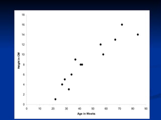
  • 9. 0 2 4 6 8 10 12 14 16 18 0 10 20 30 40 50 60 70 80 90 Age in Weeks Height in CM
  • 12. Y X Y X Y Y X X Linear relationships Curvilinear relationships Linear Correlation Linear Correlation  Slide from: Statistics for Managers Using Microsoft® Excel 4th Edition, 2004 Prentice-Hall
  • 13. Y X Y X Y Y X X Strong relationships Weak relationships Linear Correlation Linear Correlation  lide from: Statistics for Managers Using Microsoft® Excel 4th Edition, 2004 Prentice-Hall
  • 14. Correlation Coefficient Correlation Coefficient Statistic showing the degree of relation between two variables
  • 15. Simple Correlation coefficient Simple Correlation coefficient (r) (r)  It is also called Pearson's correlation It is also called Pearson's correlation or product moment correlation or product moment correlation coefficient. coefficient.  It measures the It measures the nature nature and and strength strength between two variables of between two variables of the the quantitative quantitative type. type.
  • 16. The The sign sign of of r r denotes the nature of denotes the nature of association association while the while the value value of of r r denotes the denotes the strength of association. strength of association.
  • 17.  If the sign is If the sign is +ve +ve this means the relation this means the relation is is direct direct (an increase in one variable is (an increase in one variable is associated with an increase in the associated with an increase in the other variable and a decrease in one other variable and a decrease in one variable is associated with a variable is associated with a decrease in the other variable). decrease in the other variable).  While if the sign is While if the sign is -ve -ve this means an this means an inverse or indirect inverse or indirect relationship (which relationship (which means an increase in one variable is means an increase in one variable is associated with a decrease in the other). associated with a decrease in the other).
  • 18.  The value of r ranges between ( -1) and ( +1) The value of r ranges between ( -1) and ( +1)  The value of r denotes the strength of the The value of r denotes the strength of the association as illustrated association as illustrated by the following diagram. by the following diagram. - 1 1 0 -0.25 -0.75 0.75 0.25 strong strong intermediate intermediate weak weak no relation perfect correlation perfect correlation Direct indirect
  • 19. If If r r = Zero = Zero this means no association or this means no association or correlation between the two variables. correlation between the two variables. If If 0 < 0 < r r < 0.25 < 0.25 = weak correlation. = weak correlation. If If 0.25 ≤ 0.25 ≤ r r < 0.75 < 0.75 = intermediate correlation. = intermediate correlation. If If 0.75 ≤ 0.75 ≤ r r < 1 < 1 = strong correlation. = strong correlation. If If r r = l = l = perfect correlation. = perfect correlation.
  • 20.                            n y) ( y . n x) ( x n y x xy r 2 2 2 2 How to compute the simple correlation coefficient (r)
  • 21. Example Example : : A sample of 6 children was selected, data about their A sample of 6 children was selected, data about their age in years and weight in kilograms was recorded as age in years and weight in kilograms was recorded as shown in the following table . It is required to find the shown in the following table . It is required to find the correlation between age and weight. correlation between age and weight. serial No Age (years) Weight (Kg) 1 7 12 2 6 8 3 8 12 4 5 10 5 6 11 6 9 13
  • 22. These 2 variables are of the quantitative type, one These 2 variables are of the quantitative type, one variable (Age) is called the independent and variable (Age) is called the independent and denoted as (X) variable and the other (weight) denoted as (X) variable and the other (weight) is called the dependent and denoted as (Y) is called the dependent and denoted as (Y) variables to find the relation between age and variables to find the relation between age and weight compute the simple correlation coefficient weight compute the simple correlation coefficient using the following formula: using the following formula:                            n y) ( y . n x) ( x n y x xy r 2 2 2 2
  • 24. r = 0.759 r = 0.759 strong direct correlation strong direct correlation                  6 (66) 742 . 6 (41) 291 6 66 41 461 r 2 2
  • 25. EXAMPLE: Relationship between Anxiety and EXAMPLE: Relationship between Anxiety and Test Scores Test Scores Anxiety Anxiety ( ( X X ) ) Test Test score (Y) score (Y) X X2 2 Y Y2 2 XY XY 10 10 2 2 100 100 4 4 20 20 8 8 3 3 64 64 9 9 24 24 2 2 9 9 4 4 81 81 18 18 1 1 7 7 1 1 49 49 7 7 5 5 6 6 25 25 36 36 30 30 6 6 5 5 36 36 25 25 30 30 ∑ ∑ X = 32 X = 32 ∑ ∑ Y = 32 Y = 32 ∑ ∑ X X2 2 = 230 = 230 ∑ ∑ Y Y2 2 = 204 = 204 ∑ ∑ XY=129 XY=129
  • 26. Calculating Correlation Coefficient Calculating Correlation Coefficient    94 . ) 200 )( 356 ( 1024 774 32 ) 204 ( 6 32 ) 230 ( 6 ) 32 )( 32 ( ) 129 )( 6 ( 2 2         r r = - 0.94 Indirect strong correlation
  • 27. 27 Coefficient of Coefficient of Determination Determination It is often difficult to interpret r without some familiarity with the expected values of r . A more appropriate measure to use when interest lies in the dependence of Y on X, is the Coefficient of Determination, R2 . It measures the proportion of variation in Y that is explained by X, and is often expressed as a percentage .
  • 28. 28 Using anova to find R Using anova to find R2 2 Anova (for 93 rural female headed HHs) of log consumption expenditure versus number of persons per sleeping room is : Source d.f. S.S. M.S. F Prob. Regression 1 4.890 4.890 21.9 0.000 Residual 91 20.342 0.2235 Total 92 25.231 0.2743 R2 = Regre. S.S. / Total S.S. = 4.89/25.23 = 0.194
  • 29. 29 Interpretation of R Interpretation of R2 2 From above, we can say that 19.4% of the variability in the income poverty proxy measure is accounted for by the number of persons per sleeping room . Clearly there are many other factors that influence the poverty proxy since over 80% of the variability is left unexplained !
  • 30. 30 Relationship of R Relationship of R2 2 to r to r When there is just one explanatory variable being considered (as in above example), the squared value of r equals R2 . In the above example , value of r = -  0.194 = - 0.44 The negative value is used when taking the square root because the graph indicates a negative relationship (see next slide) .
  • 31. 31 Plot of poverty proxy measure vs. persons Plot of poverty proxy measure vs. persons per sleeping room per sleeping room
  • 32. 32 Benefits of R Benefits of R2 2 and r and r • r is useful as an initial exploratory tool when several variables are being considered. The sign of r gives the direction of the association . • R2 is useful in regression studies to check how much of the variability in the key response can be explained . • R2 is most valuable when there is more than one explanatory variable. High values of R2 are particularly useful when using the model for predictions !
  • 33. 33 Limitations of r Limitations of r • Observe that seemingly high values of r, e.g. r=0.70, explain only about 50% of the variability in the response variable y. So take care when interpreting correlation coefficients . • a low value for r does not necessarily imply absence of a relationship – could be a curved relationship! So plotting the data is crucial ! • Tests exist for testing there is no association. But depending on the sample size, even low values of r, e.g. r=0.20 can give significant results – not a very useful finding !
  • 34. 34 Limitations of R Limitations of R2 2 • Note that R2 is only a descriptive measure to give a quick assessment of the model. Other methods exist for assessing the goodness of fit of the model . • Adding explanatory variables to the model always increases R2 . Hence in practice, it is more usual to look at the adjusted R2 • The adjusted R2 is calculated as 1 ( – Residual M.S./Total M.S ). As with R2 , the adjusted R2 is often expressed as a percentage .
  • 35. Spearman Rank Correlation Coefficient (r Spearman Rank Correlation Coefficient (rs s) ) It is a non-parametric measure of correlation. It is a non-parametric measure of correlation. This procedure makes use of the two sets of This procedure makes use of the two sets of ranks that may be assigned to the sample values ranks that may be assigned to the sample values of x and Y. of x and Y. Spearman Rank correlation coefficient could be Spearman Rank correlation coefficient could be computed in the following cases: computed in the following cases: Both variables are quantitative. Both variables are quantitative. Both variables are qualitative ordinal. Both variables are qualitative ordinal. One variable is quantitative and the other is qualitative One variable is quantitative and the other is qualitative ordinal. ordinal.
  • 36. Procedure Procedure : : 1. 1. Rank the values of X from 1 to n where n Rank the values of X from 1 to n where n is the numbers of pairs of values of X and is the numbers of pairs of values of X and Y in the sample. Y in the sample. 2. 2. Rank the values of Y from 1 to n. Rank the values of Y from 1 to n. 3. 3. Compute the value of di for each pair of Compute the value of di for each pair of observation by subtracting the rank of Yi observation by subtracting the rank of Yi from the rank of Xi from the rank of Xi 4. 4. Square each di and compute ∑di2 which Square each di and compute ∑di2 which is the sum of the squared values. is the sum of the squared values.
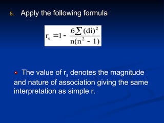
  • 37. 5. 5. Apply the following formula Apply the following formula 1) n(n (di) 6 1 r 2 2 s     The value of rs denotes the magnitude and nature of association giving the same interpretation as simple r.
  • 38. Example Example In a study of the relationship between level In a study of the relationship between level education and income the following data was education and income the following data was obtained. Find the relationship between them and obtained. Find the relationship between them and comment. comment. sample numbers level education (X) Income (Y) A Preparatory. Preparatory. 25 B Primary. Primary. 10 C University. University. 8 D secondary secondary 10 E secondary secondary 15 F illit illiterate erate 50 G University. University. 60
  • 40. Comment: Comment: There is an indirect weak correlation There is an indirect weak correlation between level of education and income. between level of education and income. 1 . 0 ) 48 ( 7 64 6 1      s r
  • 42. Regression Analyses Regression Analyses Regression: Technique concerned with predicting some variables by knowing others The process of predicting variable Y using variable X
  • 43. Regression Regression  Uses a variable (x) to predict some outcome Uses a variable (x) to predict some outcome variable (y) variable (y)  Tells you how values in y change as a function Tells you how values in y change as a function of changes in values of x of changes in values of x
  • 44. Correlation and Regression Correlation and Regression  Correlation describes the strength of a Correlation describes the strength of a linear relationship between two variables  Linear means “straight line”  Regression tells us how to draw the straight line described by the correlation
  • 45. Regression  Calculates the “best-fit” line for a certain set of data Calculates the “best-fit” line for a certain set of data The regression line makes the sum of the squares of The regression line makes the sum of the squares of the residuals smaller than for any other line the residuals smaller than for any other line Regression minimizes residuals 80 100 120 140 160 180 200 220 60 70 80 90 100 110 120 Wt (kg)
  • 46. By using the least squares method (a procedure By using the least squares method (a procedure that minimizes the vertical deviations of plotted that minimizes the vertical deviations of plotted points surrounding a straight line) we are points surrounding a straight line) we are able to construct a best fitting straight line to the able to construct a best fitting straight line to the scatter diagram points and then formulate a scatter diagram points and then formulate a regression equation in the form of: regression equation in the form of:         n x) ( x n y x xy b 2 2 1 x b - y a  b bX a ŷ  
  • 47. Regression Equation  Regression equation describes the regression line mathematically  Intercept  Slope 80 100 120 140 160 180 200 220 60 70 80 90 100 110 120 Wt (kg) SBP(mmHg)
  • 48. Linear Equations Linear Equations Y Y = bX + a a = Y-intercept X Change in Y Change in X b = Slope bX a ŷ  
  • 49. Hours studying and grades Hours studying and grades
  • 50. Regressing grades on hours grades on hours Linear Regression 2.00 4.00 6.00 8.00 10.00 Number of hours spent studying 70.00 80.00 90.00             Final grade in course = 59.95 + 3.17 * study R-Square = 0.88 Predicted final grade in class = 59.95 + 3.17*(number of hours you study per week)
  • 51. Predict the final grade of Predict the final grade of … …  Someone who studies for 12 hours  Final grade = 59.95 + (3.17*12)  Final grade = 97.99  Someone who studies for 1 hour:  Final grade = 59.95 + (3.17*1)  Final grade = 63.12 Predicted final grade in class = 59.95 + 3.17*(hours of study)
  • 52. Exercise Exercise A sample of 6 persons was selected the A sample of 6 persons was selected the value of their age ( x variable) and their value of their age ( x variable) and their weight is demonstrated in the following weight is demonstrated in the following table. Find the regression equation and table. Find the regression equation and what is the predicted weight when age is what is the predicted weight when age is 8.5 years 8.5 years. .
  • 53. Serial no . Age (x) Weight (y) 1 2 3 4 5 6 7 6 8 5 6 9 12 8 12 10 11 13
  • 54. Answer Answer Serial no . Age (x) Weight (y) xy X2 Y2 1 2 3 4 5 6 7 6 8 5 6 9 12 8 12 10 11 13 84 48 96 50 66 117 49 36 64 25 36 81 144 64 144 100 121 169 Total 41 66 461 291 742
  • 57. 11.4 11.6 11.8 12 12.2 12.4 12.6 7 7.5 8 8.5 9 Age (in years) Weight (in Kg) we create a regression line by plotting two estimated values for y against their X component, then extending the line right and left.
  • 58. Exercise 2 Exercise 2 The following are the The following are the age (in years) and age (in years) and systolic blood systolic blood pressure of 20 pressure of 20 apparently healthy apparently healthy adults. adults. Age (x) B.P (y) Age (x) B.P (y) 20 43 63 26 53 31 58 46 58 70 120 128 141 126 134 128 136 132 140 144 46 53 60 20 63 43 26 19 31 23 128 136 146 124 143 130 124 121 126 123
  • 59. Find the correlation between age Find the correlation between age and blood pressure using simple and blood pressure using simple and Spearman's correlation and Spearman's correlation coefficients, and comment. coefficients, and comment. Find the regression equation? Find the regression equation? What is the predicted blood What is the predicted blood pressure for a man aging 25 years? pressure for a man aging 25 years?
  • 62.         n x) ( x n y x xy b 2 2 1 4547 . 0 20 852 41678 20 2630 852 114486 2     = =112.13 + 0.4547 x for age 25 B.P = 112.13 + 0.4547 * 25=123.49 = 123.5 mm hg ŷ
  • 63. Multiple Regression Multiple regression analysis is a straightforward extension of simple regression analysis which allows more than one independent variable.