


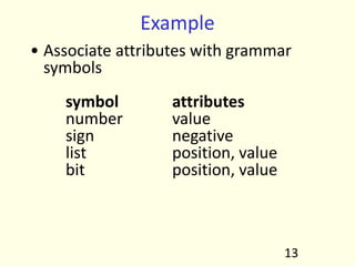
![Bootstrapping
• Compiler is a complex program and should not be
written in assembly language
• How to write compiler for a language in the same
language (first time!)?
• First time this experiment was done for Lisp
• Initially, Lisp was used as a notation for writing
functions.
• Functions were then hand translated into
assembly language and executed
• McCarthy wrote a function eval[e] in Lisp that
took a Lisp expression e as an argument
• The function was later hand translated and it
became an interpreter for Lisp
46](https://image.slidesharecdn.com/cs-321compilerdesignppt-250417035219-2e518472/85/CS-321-Compiler-Design-computer-engineering-PPT-pdf-72-320.jpg)


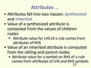
![Top down Parsing
• Following grammar generates types of
Pascal
type Æ simple
| n id
| array [ simple] of type
simple Æ integer
| char
| num dotdot num
1](https://image.slidesharecdn.com/cs-321compilerdesignppt-250417035219-2e518472/85/CS-321-Compiler-Design-computer-engineering-PPT-pdf-143-320.jpg)

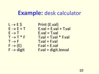
![• Parse
array [ num dotdot num ] of integer
• Cannot proceed as non terminal “simple” never generates
a string beginning with token “array”. Therefore, requires
back-tracking.
• Back-tracking is not desirable, therefore, take help of a
“look-ahead” token. The current token is treated as look-
ahead token. (restricts the class of grammars)
3
type
simple
Start symbol
Expanded using the
rule type Æ simple](https://image.slidesharecdn.com/cs-321compilerdesignppt-250417035219-2e518472/85/CS-321-Compiler-Design-computer-engineering-PPT-pdf-145-320.jpg)
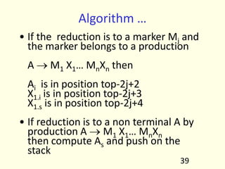
![4
array [ num dotdot num ] of integer
type
simple ] type
[
array
dotdot
num num simple
integer
look-ahead
of
Start symbol
Expand using the rule
type Æ array [ simple ] of type
Left most non terminal
Expand using the rule
Simple Æ num dotdot num
Left most non terminal
Expand using the rule
type Æ simple
Left most non terminal
Expand using the rule
simple Æ integer
all the tokens exhausted
Parsing completed](https://image.slidesharecdn.com/cs-321compilerdesignppt-250417035219-2e518472/85/CS-321-Compiler-Design-computer-engineering-PPT-pdf-146-320.jpg)

![Define a procedure for each non terminal
procedure type;
if lookahead in {integer, char, num}
then simple
else if lookahead = n
then begin match( n );
match(id)
end
else if lookahead = array
then begin match(array);
match([);
simple;
match(]);
match(of);
type
end
else error;
6](https://image.slidesharecdn.com/cs-321compilerdesignppt-250417035219-2e518472/85/CS-321-Compiler-Design-computer-engineering-PPT-pdf-148-320.jpg)


![Parsing algorithm
• The parser considers 'X' the symbol on top of stack, and 'a' the
current input symbol
• These two symbols determine the action to be taken by the parser
• Assume that '$' is a special token that is at the bottom of the stack
and terminates the input string
if X = a = $ then halt
if X = a ≠ $ then pop(x) and ip++
if X is a non terminal
then if M[X,a] = {X Æ UVW}
then begin pop(X); push(W,V,U)
end
else error
20](https://image.slidesharecdn.com/cs-321compilerdesignppt-250417035219-2e518472/85/CS-321-Compiler-Design-computer-engineering-PPT-pdf-162-320.jpg)


![Construction of parse table
• for each production A Æ α do
– for each terminal ‘a’ in first(α)
M[A,a] = A Æ α
– If Є is in First(α)
M[A,b] = A Æ α
for each terminal b in follow(A)
– If ε is in First(α) and $ is in follow(A)
M[A,$] = A Æ α
• A grammar whose parse table has no multiple entries is called LL(1)
28](https://image.slidesharecdn.com/cs-321compilerdesignppt-250417035219-2e518472/85/CS-321-Compiler-Design-computer-engineering-PPT-pdf-170-320.jpg)


![Error Recovery in LL(1) parser
• Error occurs when a parse table entry M[A,a] is empty
• Skip symbols in the input until a token in a selected set
(synch) appears
• Place symbols in follow(A) in synch set. Skip tokens until
an element in follow(A) is seen.
Pop(A) and continue parsing
• Add symbol in first(A) in synch set. Then it may be
possible to resume parsing according to A if a symbol in
first(A) appears in input.
36](https://image.slidesharecdn.com/cs-321compilerdesignppt-250417035219-2e518472/85/CS-321-Compiler-Design-computer-engineering-PPT-pdf-178-320.jpg)


![24
Actions in an LR (shift reduce) parser
• Assume Si is top of stack and ai is current
input symbol
• Action [Si,ai] can have four values
1. sj: shift ai to the stack, goto state Sj
2. rk: reduce by rule number k
3. acc: Accept
4. err: Error (empty cells in the table)](https://image.slidesharecdn.com/cs-321compilerdesignppt-250417035219-2e518472/85/CS-321-Compiler-Design-computer-engineering-PPT-pdf-203-320.jpg)
![25
Driving the LR parser
Stack: S0X1S1X2…XmSm Input: aiai+1…an$
• If action[Sm,ai] = shift S
Then the configuration becomes
Stack: S0X1S1……XmSmaiS Input: ai+1…an$
• If action[Sm,ai] = reduce AÆβ
Then the configuration becomes
Stack: S0X1S1…Xm-rSm-r AS Input: aiai+1…an$
Where r = |β| and S = goto[Sm-r,A]](https://image.slidesharecdn.com/cs-321compilerdesignppt-250417035219-2e518472/85/CS-321-Compiler-Design-computer-engineering-PPT-pdf-204-320.jpg)
![26
Driving the LR parser
Stack: S0X1S1X2…XmSm Input: aiai+1…an$
• If action[Sm,ai] = accept
Then parsing is completed. HALT
• If action[Sm,ai] = error (or empty cell)
Then invoke error recovery routine.](https://image.slidesharecdn.com/cs-321compilerdesignppt-250417035219-2e518472/85/CS-321-Compiler-Design-computer-engineering-PPT-pdf-205-320.jpg)


![29
LR parsing Algorithm
Initial state: Stack: S0 Input: w$
while (1) {
if (action[S,a] = shift S’) {
push(a); push(S’); ip++
} else if (action[S,a] = reduce AÆβ) {
pop (2*|β|) symbols;
push(A); push (goto*S’’,A+)
(S’’ is the state at stack top after popping symbols)
} else if (action[S,a] = accept) {
exit
} else { error }](https://image.slidesharecdn.com/cs-321compilerdesignppt-250417035219-2e518472/85/CS-321-Compiler-Design-computer-engineering-PPT-pdf-208-320.jpg)


![55
Construct SLR parse table
• Construct C={I0, …, In} the collection of
sets of LR(0) items
• If AÆα.aβ is in Ii and goto(Ii,a) = Ij
then action[i,a] = shift j
• If AÆα. is in Ii
then action[i,a] = reduce AÆα for all a in
follow(A)
• If S'ÆS. is in Ii then action[i,$] = accept
• If goto(Ii,A) = Ij
then goto[i,A]=j for all non terminals A
• All entries not defined are errors](https://image.slidesharecdn.com/cs-321compilerdesignppt-250417035219-2e518472/85/CS-321-Compiler-Design-computer-engineering-PPT-pdf-234-320.jpg)


![59
= * id $ S L R
0 s4 s5 1 2 3
1 acc
2 s6,r6 r6
3 r3
4 s4 s5 8 7
5 r5 r5
6 s4 s5 8 9
7 r4 r4
8 r6 r6
9 r2
SLR parse table for the grammar
The table has multiple entries in action[2,=]](https://image.slidesharecdn.com/cs-321compilerdesignppt-250417035219-2e518472/85/CS-321-Compiler-Design-computer-engineering-PPT-pdf-238-320.jpg)
![60
• There is both a shift and a reduce entry in
action[2,=]. Therefore state 2 has a shift-
reduce conflict on symbol “=“, However,
the grammar is not ambiguous.
• Parse id=id assuming reduce action is taken
in [2,=]
Stack input action
0 id=id shift 5
0 id 5 =id reduce by LÆid
0 L 2 =id reduce by RÆL
0 R 3 =id error](https://image.slidesharecdn.com/cs-321compilerdesignppt-250417035219-2e518472/85/CS-321-Compiler-Design-computer-engineering-PPT-pdf-239-320.jpg)
![61
• if shift action is taken in [2,=]
Stack input action
0 id=id$ shift 5
0 id 5 =id$ reduce by LÆid
0 L 2 =id$ shift 6
0 L 2 = 6 id$ shift 5
0 L 2 = 6 id 5 $ reduce by LÆid
0 L 2 = 6 L 8 $ reduce by RÆL
0 L 2 = 6 R 9 $ reduce by SÆL=R
0 S 1 $ ACCEPT](https://image.slidesharecdn.com/cs-321compilerdesignppt-250417035219-2e518472/85/CS-321-Compiler-Design-computer-engineering-PPT-pdf-240-320.jpg)
![62
Problems in SLR parsing
• No sentential form of this grammar can start with R=…
• However, the reduce action in action[2,=] generates a
sentential form starting with R=
• Therefore, the reduce action is incorrect
• In SLR parsing method state i calls for reduction on
symbol “a”, by rule AÆα if Ii contains [AÆα.+ and “a” is
in follow(A)
• However, when state I appears on the top of the stack,
the viable prefix βα on the stack may be such that βA
can not be followed by symbol “a” in any right
sentential form
• Thus, the reduction by the rule AÆα on symbol “a” is
invalid
• SLR parsers cannot remember the left context](https://image.slidesharecdn.com/cs-321compilerdesignppt-250417035219-2e518472/85/CS-321-Compiler-Design-computer-engineering-PPT-pdf-241-320.jpg)
![63
Canonical LR Parsing
• Carry extra information in the state so that
wrong reductions by A Æ α will be ruled out
• Redefine LR items to include a terminal
symbol as a second component (look ahead
symbol)
• The general form of the item becomes [A Æ
α.β, a] which is called LR(1) item.
• Item [A Æ α., a] calls for reduction only if
next input is a. The set of symbols “a”s will
be a subset of Follow(A).](https://image.slidesharecdn.com/cs-321compilerdesignppt-250417035219-2e518472/85/CS-321-Compiler-Design-computer-engineering-PPT-pdf-242-320.jpg)
![64
Closure(I)
repeat
for each item [A Æ α.Bβ, a] in I
for each production B Æ γ in G'
and for each terminal b in First(βa)
add item [B Æ .γ, b] to I
until no more additions to I](https://image.slidesharecdn.com/cs-321compilerdesignppt-250417035219-2e518472/85/CS-321-Compiler-Design-computer-engineering-PPT-pdf-243-320.jpg)
![65
Example
Consider the following grammar
S‘Æ S
S Æ CC
C Æ cC | d
Compute closure(I) where I=,*S’ Æ .S, $]}
S‘Æ .S, $
S Æ .CC, $
C Æ .cC, c
C Æ .cC, d
C Æ .d, c
C Æ .d, d](https://image.slidesharecdn.com/cs-321compilerdesignppt-250417035219-2e518472/85/CS-321-Compiler-Design-computer-engineering-PPT-pdf-244-320.jpg)

![67
Construction of Canonical LR
parse table
• Construct C={I0, …,In} the sets of LR(1) items.
• If [A Æ α.aβ, b] is in Ii and goto(Ii, a)=Ij
then action[i,a]=shift j
• If [A Æ α., a] is in Ii
then action[i,a] reduce A Æ α
• If [S′ Æ S., $] is in Ii
then action[i,$] = accept
• If goto(Ii, A) = Ij then goto[i,A] = j for all non terminals A](https://image.slidesharecdn.com/cs-321compilerdesignppt-250417035219-2e518472/85/CS-321-Compiler-Design-computer-engineering-PPT-pdf-246-320.jpg)


![74
Notes on LALR parse table…
• Merging items may result into conflicts in LALR parsers
which did not exist in LR parsers
• New conflicts can not be of shift reduce kind:
– Assume there is a shift reduce conflict in some state of LALR
parser with items
{[XÆα.,a],[YÆγ.aβ,b]}
– Then there must have been a state in the LR parser with the same
core
– Contradiction; because LR parser did not have conflicts
• LALR parser can have new reduce-reduce conflicts
– Assume states
{[XÆα., a], [YÆβ., b]} and {[XÆα., b], [YÆβ., a]}
– Merging the two states produces
{[XÆα., a/b], [YÆβ., a/b]}](https://image.slidesharecdn.com/cs-321compilerdesignppt-250417035219-2e518472/85/CS-321-Compiler-Design-computer-engineering-PPT-pdf-253-320.jpg)

![76
Error Recovery
• An error is detected when an entry in the action table is found to be
empty.
• Panic mode error recovery can be implemented as follows:
– scan down the stack until a state S with a goto on a particular
nonterminal A is found.
– discard zero or more input symbols until a symbol a is found that can
legitimately follow A.
– stack the state goto[S,A] and resume parsing.
• Choice of A: Normally these are non terminals representing major
program pieces such as an expression, statement or a block. For
example if A is the nonterminal stmt, a might be semicolon or end.](https://image.slidesharecdn.com/cs-321compilerdesignppt-250417035219-2e518472/85/CS-321-Compiler-Design-computer-engineering-PPT-pdf-255-320.jpg)


![Compiler needs to know?
• Whether a variable has been declared?
• Are there variables which have not been
declared?
• What is the type of the variable?
• Whether a variable is a scalar, an array, or a
function?
• What declaration of the variable does each
reference use?
• If an expression is type consistent?
• If an array use like A[i,j,k] is consistent with
the declaration? Does it have three
dimensions?
4](https://image.slidesharecdn.com/cs-321compilerdesignppt-250417035219-2e518472/85/CS-321-Compiler-Design-computer-engineering-PPT-pdf-262-320.jpg)


![E → E + T val(ntop) = val(top-2) + val(top)
In YACC
E → E + T $$ = $1 + $3
$$ maps to val[top – r + 1]
$k maps to val[top – r + k]
r=#symbols on RHS ( here 3)
$$ = $1 is the default action in YACC
YACC Terminology](https://image.slidesharecdn.com/cs-321compilerdesignppt-250417035219-2e518472/85/CS-321-Compiler-Design-computer-engineering-PPT-pdf-300-320.jpg)


![Example …
• Every time a reduction to L is made value of T
type is just below it
• Use the fact that T.val (type information) is at a
known place in the stack
• When production L o id is applied, id.entry is at
the top of the stack and T.type is just below it,
therefore,
addtype(id.entry,L.in) œ
addtype(val[top], val[top-1])
• Similarly when production L o L1 , id is applied
id.entry is at the top of the stack and T.type is
three places below it, therefore,
addtype(id.entry, L.in) œ
addtype(val[top],val[top-3])
33](https://image.slidesharecdn.com/cs-321compilerdesignppt-250417035219-2e518472/85/CS-321-Compiler-Design-computer-engineering-PPT-pdf-313-320.jpg)
![Example …
Therefore, the translation scheme becomes
D o T L
T o int val[top] =integer
T o real val[top] =real
L o L,id addtype(val[top], val[top-3])
L o id addtype(val[top], val[top-1])
34](https://image.slidesharecdn.com/cs-321compilerdesignppt-250417035219-2e518472/85/CS-321-Compiler-Design-computer-engineering-PPT-pdf-314-320.jpg)
![Simulating the evaluation of
inherited attributes
• The scheme works only if grammar allows
position of attribute to be predicted.
• Consider the grammar
S o aAC Ci = As
S o bABC Ci = As
C o c Cs = g(Ci)
• C inherits As
• there may or may not be a B between A
and C on the stack when reduction by rule
CÆc takes place
• When reduction by C o c is performed the
value of Ci is either in [top-1] or [top-2]
35](https://image.slidesharecdn.com/cs-321compilerdesignppt-250417035219-2e518472/85/CS-321-Compiler-Design-computer-engineering-PPT-pdf-315-320.jpg)
![Simulating the evaluation …
• Insert a marker M just before C in the
second rule and change rules to
S o aAC Ci = As
S o bABMC Mi = As; Ci = Ms
C o c Cs = g(Ci)
M o ε Ms = Mi
• When production M o ε is applied we have
Ms = Mi = As
• Therefore value of Ci is always at val[top-1]
36](https://image.slidesharecdn.com/cs-321compilerdesignppt-250417035219-2e518472/85/CS-321-Compiler-Design-computer-engineering-PPT-pdf-316-320.jpg)


![Example
• Consider following definition
D oT L L.in := T.type
T o real T.type := real
T o int T.type := int
L o L1,I L1.in :=L.in; I.in=L.in
L o I I.in = L.in
I o I1[num] I1.in=array(numeral, I.in)
I o id addtype(id.entry,I.in)
41](https://image.slidesharecdn.com/cs-321compilerdesignppt-250417035219-2e518472/85/CS-321-Compiler-Design-computer-engineering-PPT-pdf-321-320.jpg)
![Consider string int x[3], y[5]
its parse tree and dependence graph
42
D
T L
int L , I
I
I [ num ]
id
I [ num ]
id
3
5
x
y
1 2
3
4
5
6
7
8
9](https://image.slidesharecdn.com/cs-321compilerdesignppt-250417035219-2e518472/85/CS-321-Compiler-Design-computer-engineering-PPT-pdf-322-320.jpg)


![Type Constructors
• Array: if T is a type expression then array(I, T)
is a type expression denoting the type of an
array with elements of type T and index set I
int A[10];
A can have type expression array(0 .. 9, integer)
• C does not use this type, but uses
equivalent of int*
• Product: if T1 and T2 are type expressions
then their Cartesian product T1 * T2 is a type
expression
• Pair/tuple
7](https://image.slidesharecdn.com/cs-321compilerdesignppt-250417035219-2e518472/85/CS-321-Compiler-Design-computer-engineering-PPT-pdf-333-320.jpg)
![Type constructors …
• Records: it applies to a tuple formed from field
names and field types. Consider the declaration
type row = record
addr : integer;
lexeme : array [1 .. 15] of char
end;
var table: array [1 .. 10] of row;
• The type row has type expression
record ((addr * integer) * (lexeme * array(1 .. 15,
char)))
and type expression of table is array(1 .. 10, row)
8](https://image.slidesharecdn.com/cs-321compilerdesignppt-250417035219-2e518472/85/CS-321-Compiler-Design-computer-engineering-PPT-pdf-334-320.jpg)

![Specifications of a type checker
• Consider a language which consists
of a sequence of declarations
followed by a single expression
P → D ; E
D → D ; D | id : T
T → char | integer | T[num] | T*
E → literal | num | E%E | E [E] | *E
10](https://image.slidesharecdn.com/cs-321compilerdesignppt-250417035219-2e518472/85/CS-321-Compiler-Design-computer-engineering-PPT-pdf-336-320.jpg)
![Specifications of a type checker …
• A program generated by this grammar is
key : integer;
key %1999
• Assume following:
– basic types are char, int, type-error
– all arrays start at 0
– char[256] has type expression
array(0 .. 255, char)
11](https://image.slidesharecdn.com/cs-321compilerdesignppt-250417035219-2e518472/85/CS-321-Compiler-Design-computer-engineering-PPT-pdf-337-320.jpg)
![Rules for Symbol Table entry
D Æ id : T addtype(id.entry, T.type)
T Æ char T.type = char
T Æ integer T.type = int
T Æ T1* T.type = pointer(T1.type)
T Æ T1 [num] T.type = array(0..num-1, T1.type)
12](https://image.slidesharecdn.com/cs-321compilerdesignppt-250417035219-2e518472/85/CS-321-Compiler-Design-computer-engineering-PPT-pdf-338-320.jpg)

![Type checking for expressions
E → literal E.type = char
E → num E.type = integer
E → id E.type = lookup(id.entry)
E → E1 % E2 E.type = if E1.type == integer and E2.type==integer
then integer
else type_error
E → E1[E2] E.type = if E2.type==integer and E1.type==array(s,t)
then t
else type_error
E → *E1 E.type = if E1.type==pointer(t)
then t
else type_error
14](https://image.slidesharecdn.com/cs-321compilerdesignppt-250417035219-2e518472/85/CS-321-Compiler-Design-computer-engineering-PPT-pdf-340-320.jpg)
![Type checking for expressions
E → literal E.type = char
E → num E.type = integer
E → id E.type = lookup(id.entry)
E → E1 % E2 E.type = if E1.type == integer and E2.type==integer
then integer
else type_error
E → E1[E2] E.type = if E2.type==integer and E1.type==array(s,t)
then t
else type_error
E → *E1 E.type = if E1.type==pointer(t)
then t
else type_error
15](https://image.slidesharecdn.com/cs-321compilerdesignppt-250417035219-2e518472/85/CS-321-Compiler-Design-computer-engineering-PPT-pdf-341-320.jpg)


![Reading assignment
• Rest of Section 6.6 and Section 6.7 of Old
Dragonbook [Aho, Sethi and Ullman]
44](https://image.slidesharecdn.com/cs-321compilerdesignppt-250417035219-2e518472/85/CS-321-Compiler-Design-computer-engineering-PPT-pdf-370-320.jpg)


![float a[20][10];
use a[i][j+2]
HIR
t1Åa[i,j+2]
MIR
t1Å j+2
t2Å i*20
t3Å t1+t2
t4Å 4*t3
t5Å addr a
t6Å t4+t5
t7Å*t6
LIR
r1Å [fp-4]
r2Å r1+2
r3Å [fp-8]
r4Å r3*20
r5Å r4+r2
r6Å 4*r5
r7Åfp-216
f1Å [r7+r6]
7](https://image.slidesharecdn.com/cs-321compilerdesignppt-250417035219-2e518472/85/CS-321-Compiler-Design-computer-engineering-PPT-pdf-377-320.jpg)


![Three address instructions
• Assignment
– x = y op z
– x = op y
– x = y
• Jump
– goto L
– if x relop y goto L
• Indexed assignment
– x = y[i]
– x[i] = y
• Function
– param x
– call p,n
– return y
• Pointer
– x = &y
– x = *y
– *x = y
17](https://image.slidesharecdn.com/cs-321compilerdesignppt-250417035219-2e518472/85/CS-321-Compiler-Design-computer-engineering-PPT-pdf-385-320.jpg)


![Example
program sort;
var a : array[0..10] of integer;
procedure readarray;
var i :integer;
:
procedure exchange(i, j
:integer)
:
36
procedure quicksort (m, n :integer);
var i :integer;
function partition (y, z
:integer) :integer;
var i, j, x, v :integer;
:
i:= partition (m,n);
quicksort (m,i-1);
quicksort(i+1, n);
:
begin{main}
readarray;
quicksort(1,9)
end.](https://image.slidesharecdn.com/cs-321compilerdesignppt-250417035219-2e518472/85/CS-321-Compiler-Design-computer-engineering-PPT-pdf-399-320.jpg)


![Three address code
• Assignment
– x = y op z
– x = op y
– x = y
• Jump
– goto L
– if x relop y goto L
• Indexed assignment
– x = y[i]
– x[i] = y
• Function
– param x
– call p,n
– return y
• Pointer
– x = &y
– x = *y
– *x = y
4](https://image.slidesharecdn.com/cs-321compilerdesignppt-250417035219-2e518472/85/CS-321-Compiler-Design-computer-engineering-PPT-pdf-404-320.jpg)


![Declarations …
T → array [ num ] of T1
T.type = array(num.val, T1.type)
T.width = num.val x T1.width
T → ↑T1
T.type = pointer(T1.type)
T.width = 4
14](https://image.slidesharecdn.com/cs-321compilerdesignppt-250417035219-2e518472/85/CS-321-Compiler-Design-computer-engineering-PPT-pdf-414-320.jpg)

![Example
program sort;
var a : array[1..n] of integer;
x : integer;
procedure readarray;
var i : integer;
……
procedure exchange(i,j:integers);
……
procedure quicksort(m,n : integer);
var k,v : integer;
function partition(x,y:integer):integer;
var i,j: integer;
……
……
begin{main}
……
end.
16](https://image.slidesharecdn.com/cs-321compilerdesignppt-250417035219-2e518472/85/CS-321-Compiler-Design-computer-engineering-PPT-pdf-416-320.jpg)


![Example
program sort;
var a : array[0..10] of
integer;
procedure readarray;
var i :integer;
:
function partition (y, z
:integer)
:integer;
var i, j ,x, v :integer;
:
4
procedure quicksort (m, n
:integer);
var i :integer;
:
i:= partition (m,n);
quicksort (m,i-1);
quicksort(i+1, n);
:
begin{main}
readarray;
quicksort(1,9)
end.](https://image.slidesharecdn.com/cs-321compilerdesignppt-250417035219-2e518472/85/CS-321-Compiler-Design-computer-engineering-PPT-pdf-456-320.jpg)


![Scope with nested procedures
Program sort;
var a: array[1..n] of integer;
x: integer;
procedure readarray;
var i: integer;
begin
end;
procedure exchange(i,j:integer)
begin
end;
41
procedure quicksort(m,n:integer);
var k,v : integer;
function partition(y,z:integer): integer;
var i,j: integer;
begin
end;
begin
.
end;
begin
.
end.](https://image.slidesharecdn.com/cs-321compilerdesignppt-250417035219-2e518472/85/CS-321-Compiler-Design-computer-engineering-PPT-pdf-493-320.jpg)


![Displays
• Faster access to non
locals
• Uses an array of
pointers to
activation records
• Non locals at depth i
are in the activation
record pointed to by
d[i]
51
q(1,9)
saved d[2]
q(1,3)
saved d[2]
p(1,3)
saved d[3]
e(1,3)
saved d[2]
s
d[1]
d[2]
d[3]](https://image.slidesharecdn.com/cs-321compilerdesignppt-250417035219-2e518472/85/CS-321-Compiler-Design-computer-engineering-PPT-pdf-503-320.jpg)
![Setting up Displays
• When a new activation record for a
procedure at nesting depth i is set up:
• Save the value of d[i] in the new activation
record
• Set d[i] to point to the new activation
record
• Just before an activation ends, d[i] is reset
to the saved value
52](https://image.slidesharecdn.com/cs-321compilerdesignppt-250417035219-2e518472/85/CS-321-Compiler-Design-computer-engineering-PPT-pdf-504-320.jpg)
![Justification for Displays
• Suppose procedure at depth j calls procedure at
depth i
• Case j < i then i = j + 1
– called procedure is nested within the caller
– first j elements of display need not be changed
– old value of d[i] is saved and d[i] set to the new
activation record
• Case j ≥ i
– enclosing procedure at depths 1…i-1 are same and are
left un-disturbed
– old value of d[i] is saved and d[i] points to the new
record
– display is correct as first i-1 records are not disturbed
53](https://image.slidesharecdn.com/cs-321compilerdesignppt-250417035219-2e518472/85/CS-321-Compiler-Design-computer-engineering-PPT-pdf-505-320.jpg)


![Parameter Passing …
• Call by name (used in Algol)
–names are copied
–local names are different from
names of calling procedure
–Issue:
61
swap(x, y) {
temp = x
x = y
y = temp
}
swap(i,a[i]):
temp = i
i = a[i]
a[i] = temp](https://image.slidesharecdn.com/cs-321compilerdesignppt-250417035219-2e518472/85/CS-321-Compiler-Design-computer-engineering-PPT-pdf-513-320.jpg)


![DAG representation: example
1. t1 := 4 * i
2. t2 := a[t1]
3. t3 := 4 * i
4. t4 := b[t3]
5. t5 := t2 * t4
6. t6 := prod + t5
7. prod := t6
8. t7 := i + 1
9. i := t7
10. if i <= 20 goto (1)
21
+
prod0 *
[ ] [ ]
*
i0
4
b
a +
1
20
<=
t1
t4
t5
t6
t7
(1)
t3
t2
prod
i](https://image.slidesharecdn.com/cs-321compilerdesignppt-250417035219-2e518472/85/CS-321-Compiler-Design-computer-engineering-PPT-pdf-538-320.jpg)
![Code Generation from DAG
S1 = 4 * i
S2 = addr(A)-4
S3 = S2[S1]
S4 = 4 * i
S5 = addr(B)-4
S6 = S5[S4]
S7 = S3 * S6
S8 = prod+S7
prod = S8
S9 = I+1
I = S9
If I <= 20 goto (1)
22
S1 = 4 * i
S2 = addr(A)-4
S3 = S2[S1]
S5 = addr(B)-4
S6 = S5[S4]
S7 = S3 * S6
prod = prod + S7
I = I + 1
If I <= 20 goto (1)](https://image.slidesharecdn.com/cs-321compilerdesignppt-250417035219-2e518472/85/CS-321-Compiler-Design-computer-engineering-PPT-pdf-539-320.jpg)


![An Example
gencode(/)
SUB t1,r0
gencode(*)
MOVE r0,t1
[r0,r1]
[r0,r1]
gencode(-)
[r0,r1]
gencode(+)
MUL r1,r0
gencode(+)
DIV r1,r0
[r1]
[r1]
gencode(a)
gencode(c)
[r0]
[r0]
MOVE c,r0
MOVE a,r0
ADD e,r1
ADD c,r1
gencode(b)
gencode(d)
[r1]
[r1]
MOVE d,r1
MOVE b,r1](https://image.slidesharecdn.com/cs-321compilerdesignppt-250417035219-2e518472/85/CS-321-Compiler-Design-computer-engineering-PPT-pdf-627-320.jpg)


![An Example
gencode(/)
SUB t1,r0
gencode(*)
MOVE r0,t1
[r0,r1]
[r0,r1]
gencode(-)
[r0,r1]
gencode(+)
MUL r1,r0
gencode(+)
DIV r1,r0
[r1]
[r1]
gencode(a)
gencode(c)
[r0]
[r0]
MOVE c,r0
MOVE a,r0
ADD e,r1
ADD c,r1
gencode(b)
gencode(d)
[r1]
[r1]
MOVE d,r1
MOVE b,r1](https://image.slidesharecdn.com/cs-321compilerdesignppt-250417035219-2e518472/85/CS-321-Compiler-Design-computer-engineering-PPT-pdf-734-320.jpg)


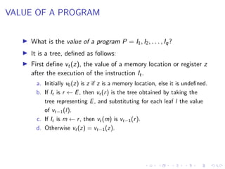
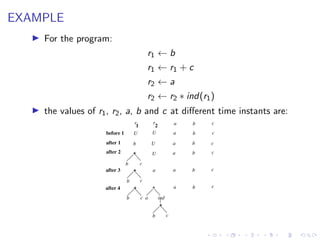
![MACHINE PROGRAM
! A machine program consists of a finite sequence of
instructions P = I1I2 . . . Iq.
! The machine program below evaluates a[i] + i ∗ b](https://image.slidesharecdn.com/cs-321compilerdesignppt-250417035219-2e518472/85/CS-321-Compiler-Design-computer-engineering-PPT-pdf-779-320.jpg)
![MACHINE PROGRAM
! A machine program consists of a finite sequence of
instructions P = I1I2 . . . Iq.
! The machine program below evaluates a[i] + i ∗ b](https://image.slidesharecdn.com/cs-321compilerdesignppt-250417035219-2e518472/85/CS-321-Compiler-Design-computer-engineering-PPT-pdf-780-320.jpg)
![MACHINE PROGRAM
! A machine program consists of a finite sequence of
instructions P = I1I2 . . . Iq.
! The machine program below evaluates a[i] + i ∗ b
r1 ← 4](https://image.slidesharecdn.com/cs-321compilerdesignppt-250417035219-2e518472/85/CS-321-Compiler-Design-computer-engineering-PPT-pdf-781-320.jpg)
![MACHINE PROGRAM
! A machine program consists of a finite sequence of
instructions P = I1I2 . . . Iq.
! The machine program below evaluates a[i] + i ∗ b
r1 ← 4
r1 ← r1 ∗ i](https://image.slidesharecdn.com/cs-321compilerdesignppt-250417035219-2e518472/85/CS-321-Compiler-Design-computer-engineering-PPT-pdf-782-320.jpg)
![MACHINE PROGRAM
! A machine program consists of a finite sequence of
instructions P = I1I2 . . . Iq.
! The machine program below evaluates a[i] + i ∗ b
r1 ← 4
r1 ← r1 ∗ i
r2 ← addr a](https://image.slidesharecdn.com/cs-321compilerdesignppt-250417035219-2e518472/85/CS-321-Compiler-Design-computer-engineering-PPT-pdf-783-320.jpg)
![MACHINE PROGRAM
! A machine program consists of a finite sequence of
instructions P = I1I2 . . . Iq.
! The machine program below evaluates a[i] + i ∗ b
r1 ← 4
r1 ← r1 ∗ i
r2 ← addr a
r2 ← r2 + r1](https://image.slidesharecdn.com/cs-321compilerdesignppt-250417035219-2e518472/85/CS-321-Compiler-Design-computer-engineering-PPT-pdf-784-320.jpg)
![MACHINE PROGRAM
! A machine program consists of a finite sequence of
instructions P = I1I2 . . . Iq.
! The machine program below evaluates a[i] + i ∗ b
r1 ← 4
r1 ← r1 ∗ i
r2 ← addr a
r2 ← r2 + r1
r2 ← ind(r2)](https://image.slidesharecdn.com/cs-321compilerdesignppt-250417035219-2e518472/85/CS-321-Compiler-Design-computer-engineering-PPT-pdf-785-320.jpg)
![MACHINE PROGRAM
! A machine program consists of a finite sequence of
instructions P = I1I2 . . . Iq.
! The machine program below evaluates a[i] + i ∗ b
r1 ← 4
r1 ← r1 ∗ i
r2 ← addr a
r2 ← r2 + r1
r2 ← ind(r2)
r3 ← i](https://image.slidesharecdn.com/cs-321compilerdesignppt-250417035219-2e518472/85/CS-321-Compiler-Design-computer-engineering-PPT-pdf-786-320.jpg)
![MACHINE PROGRAM
! A machine program consists of a finite sequence of
instructions P = I1I2 . . . Iq.
! The machine program below evaluates a[i] + i ∗ b
r1 ← 4
r1 ← r1 ∗ i
r2 ← addr a
r2 ← r2 + r1
r2 ← ind(r2)
r3 ← i
r3 ← r3 ∗ b](https://image.slidesharecdn.com/cs-321compilerdesignppt-250417035219-2e518472/85/CS-321-Compiler-Design-computer-engineering-PPT-pdf-787-320.jpg)
![MACHINE PROGRAM
! A machine program consists of a finite sequence of
instructions P = I1I2 . . . Iq.
! The machine program below evaluates a[i] + i ∗ b
r1 ← 4
r1 ← r1 ∗ i
r2 ← addr a
r2 ← r2 + r1
r2 ← ind(r2)
r3 ← i
r3 ← r3 ∗ b
r2 ← r2 + r3](https://image.slidesharecdn.com/cs-321compilerdesignppt-250417035219-2e518472/85/CS-321-Compiler-Design-computer-engineering-PPT-pdf-788-320.jpg)
![MACHINE PROGRAM
! A machine program consists of a finite sequence of
instructions P = I1I2 . . . Iq.
! The machine program below evaluates a[i] + i ∗ b
r1 ← 4
r1 ← r1 ∗ i
r2 ← addr a
r2 ← r2 + r1
r2 ← ind(r2)
r3 ← i
r3 ← r3 ∗ b
r2 ← r2 + r3](https://image.slidesharecdn.com/cs-321compilerdesignppt-250417035219-2e518472/85/CS-321-Compiler-Design-computer-engineering-PPT-pdf-789-320.jpg)


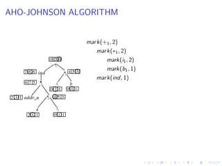
![AHO-JOHNSON ALGORITHM
Consider the subtree 4 ∗ i. For the leaf labeled 4,
1. C[1] = 1, load the constant into a register using the MOVE c,
m instruction.](https://image.slidesharecdn.com/cs-321compilerdesignppt-250417035219-2e518472/85/CS-321-Compiler-Design-computer-engineering-PPT-pdf-896-320.jpg)
![AHO-JOHNSON ALGORITHM
Consider the subtree 4 ∗ i. For the leaf labeled 4,
1. C[1] = 1, load the constant into a register using the MOVE c,
m instruction.
2. C[2] = 1, the extra register does not help.](https://image.slidesharecdn.com/cs-321compilerdesignppt-250417035219-2e518472/85/CS-321-Compiler-Design-computer-engineering-PPT-pdf-897-320.jpg)
![AHO-JOHNSON ALGORITHM
Consider the subtree 4 ∗ i. For the leaf labeled 4,
1. C[1] = 1, load the constant into a register using the MOVE c,
m instruction.
2. C[2] = 1, the extra register does not help.
3. C[0] = 2, load into a register, and then store in memory
location.](https://image.slidesharecdn.com/cs-321compilerdesignppt-250417035219-2e518472/85/CS-321-Compiler-Design-computer-engineering-PPT-pdf-898-320.jpg)
![AHO-JOHNSON ALGORITHM
Consider the subtree 4 ∗ i. For the leaf labeled 4,
1. C[1] = 1, load the constant into a register using the MOVE c,
m instruction.
2. C[2] = 1, the extra register does not help.
3. C[0] = 2, load into a register, and then store in memory
location.](https://image.slidesharecdn.com/cs-321compilerdesignppt-250417035219-2e518472/85/CS-321-Compiler-Design-computer-engineering-PPT-pdf-899-320.jpg)
![AHO-JOHNSON ALGORITHM
Consider the subtree 4 ∗ i. For the leaf labeled 4,
1. C[1] = 1, load the constant into a register using the MOVE c,
m instruction.
2. C[2] = 1, the extra register does not help.
3. C[0] = 2, load into a register, and then store in memory
location.
For the leaf labeled i,](https://image.slidesharecdn.com/cs-321compilerdesignppt-250417035219-2e518472/85/CS-321-Compiler-Design-computer-engineering-PPT-pdf-900-320.jpg)
![AHO-JOHNSON ALGORITHM
Consider the subtree 4 ∗ i. For the leaf labeled 4,
1. C[1] = 1, load the constant into a register using the MOVE c,
m instruction.
2. C[2] = 1, the extra register does not help.
3. C[0] = 2, load into a register, and then store in memory
location.
For the leaf labeled i,
1. C[1] = 1, load the variable into a register.](https://image.slidesharecdn.com/cs-321compilerdesignppt-250417035219-2e518472/85/CS-321-Compiler-Design-computer-engineering-PPT-pdf-901-320.jpg)
![AHO-JOHNSON ALGORITHM
Consider the subtree 4 ∗ i. For the leaf labeled 4,
1. C[1] = 1, load the constant into a register using the MOVE c,
m instruction.
2. C[2] = 1, the extra register does not help.
3. C[0] = 2, load into a register, and then store in memory
location.
For the leaf labeled i,
1. C[1] = 1, load the variable into a register.
2. C[2] = 1,](https://image.slidesharecdn.com/cs-321compilerdesignppt-250417035219-2e518472/85/CS-321-Compiler-Design-computer-engineering-PPT-pdf-902-320.jpg)
![AHO-JOHNSON ALGORITHM
Consider the subtree 4 ∗ i. For the leaf labeled 4,
1. C[1] = 1, load the constant into a register using the MOVE c,
m instruction.
2. C[2] = 1, the extra register does not help.
3. C[0] = 2, load into a register, and then store in memory
location.
For the leaf labeled i,
1. C[1] = 1, load the variable into a register.
2. C[2] = 1,
3. C[0] = 0, do nothing, i is already in a memory location.](https://image.slidesharecdn.com/cs-321compilerdesignppt-250417035219-2e518472/85/CS-321-Compiler-Design-computer-engineering-PPT-pdf-903-320.jpg)

![AHO-JOHNSON ALGORITHM
For the node labeled *,
1. C[2] = 3, evaluate each of the operands in registers and use
the op r1, r2 instruction.](https://image.slidesharecdn.com/cs-321compilerdesignppt-250417035219-2e518472/85/CS-321-Compiler-Design-computer-engineering-PPT-pdf-905-320.jpg)
![AHO-JOHNSON ALGORITHM
For the node labeled *,
1. C[2] = 3, evaluate each of the operands in registers and use
the op r1, r2 instruction.
2. C[0] = 4, evaluate the node using two registers as above and
store in a memory location.](https://image.slidesharecdn.com/cs-321compilerdesignppt-250417035219-2e518472/85/CS-321-Compiler-Design-computer-engineering-PPT-pdf-906-320.jpg)
![AHO-JOHNSON ALGORITHM
For the node labeled *,
1. C[2] = 3, evaluate each of the operands in registers and use
the op r1, r2 instruction.
2. C[0] = 4, evaluate the node using two registers as above and
store in a memory location.
3. C[1] =](https://image.slidesharecdn.com/cs-321compilerdesignppt-250417035219-2e518472/85/CS-321-Compiler-Design-computer-engineering-PPT-pdf-907-320.jpg)
![AHO-JOHNSON ALGORITHM
For the node labeled *,
1. C[2] = 3, evaluate each of the operands in registers and use
the op r1, r2 instruction.
2. C[0] = 4, evaluate the node using two registers as above and
store in a memory location.
3. C[1] =](https://image.slidesharecdn.com/cs-321compilerdesignppt-250417035219-2e518472/85/CS-321-Compiler-Design-computer-engineering-PPT-pdf-908-320.jpg)
![AHO-JOHNSON ALGORITHM
For the node labeled *,
1. C[2] = 3, evaluate each of the operands in registers and use
the op r1, r2 instruction.
2. C[0] = 4, evaluate the node using two registers as above and
store in a memory location.
3. C[1] = 5, notice that our machine has no op m, r instruction.
So we can use two registers to perform the operation and
store the result in a memory location releasing the registers.
When we want to use the result, we can load it in a register.
The cost in this case is C[0] + 1 = 5.](https://image.slidesharecdn.com/cs-321compilerdesignppt-250417035219-2e518472/85/CS-321-Compiler-Design-computer-engineering-PPT-pdf-909-320.jpg)


CS-321 Compiler Design computer engineering PPT.pdf
- 1. 3 Motivation • Language processing is an important component of programming • A large number of systems software and application programs require structured input – Operating Systems (command line processing) – Databases (Query language processing) – Type setting systems like Latex
- 2. 3 Motivation • Language processing is an important component of programming • A large number of systems software and application programs require structured input – Operating Systems (command line processing) – Databases (Query language processing) – Type setting systems like Latex • Software quality assurance and software testing
- 3. 4 • Where ever input has a structure one can think of language processing Motivation
- 4. 4 • Where ever input has a structure one can think of language processing • Why study compilers? – Compilers use the whole spectrum of language processing technology Motivation
- 5. 5 Expectations? • What will we learn in the course?
- 6. 6 What do we expect to achieve by the end of the course? • Knowledge to design, develop, understand, modify/enhance, and maintain compilers for (even complex!) programming languages
- 7. 6 What do we expect to achieve by the end of the course? • Knowledge to design, develop, understand, modify/enhance, and maintain compilers for (even complex!) programming languages • Confidence to use language processing technology for software development
- 8. 7 Organization of the course • Assignments 10% • Mid semester exam 20% • End semester exam 35% • Course Project 35% – Group of 2/3/4 (to be decided) • Tentative
- 9. 8 Bit of History • How are programming languages implemented? Two major strategies: – Interpreters (old and much less studied) – Compilers (very well understood with mathematical foundations)
- 10. 8 Bit of History • How are programming languages implemented? Two major strategies: – Interpreters (old and much less studied) – Compilers (very well understood with mathematical foundations) • Some environments provide both interpreter and compiler. Lisp, scheme etc. provide – Interpreter for development – Compiler for deployment –
- 11. 8 Bit of History • How are programming languages implemented? Two major strategies: – Interpreters (old and much less studied) – Compilers (very well understood with mathematical foundations) • Some environments provide both interpreter and compiler. Lisp, scheme etc. provide – Interpreter for development – Compiler for deployment • Java – Java compiler: Java to interpretable bytecode – Java JIT: bytecode to executable image
- 12. 9 Some early machines and implementations • IBM developed 704 in 1954. All programming was done in assembly language. Cost of software development far exceeded cost of hardware. Low productivity.
- 13. 9 Some early machines and implementations • IBM developed 704 in 1954. All programming was done in assembly language. Cost of software development far exceeded cost of hardware. Low productivity. • Speedcoding interpreter: programs ran about 10 times slower than hand written assembly code
- 14. 9 Some early machines and implementations • IBM developed 704 in 1954. All programming was done in assembly language. Cost of software development far exceeded cost of hardware. Low productivity. • Speedcoding interpreter: programs ran about 10 times slower than hand written assembly code • John Backus (in 1954): Proposed a program that translated high level expressions into native machine code. Skeptism all around. Most people thought it was impossible
- 15. 9 Some early machines and implementations • IBM developed 704 in 1954. All programming was done in assembly language. Cost of software development far exceeded cost of hardware. Low productivity. • Speedcoding interpreter: programs ran about 10 times slower than hand written assembly code • John Backus (in 1954): Proposed a program that translated high level expressions into native machine code. Skeptism all around. Most people thought it was impossible • Fortran I project (1954-1957): The first compiler was released
- 16. 10 Fortran I • The first compiler had a huge impact on the programming languages and computer science. The whole new field of compiler design was started
- 17. 10 Fortran I • The first compiler had a huge impact on the programming languages and computer science. The whole new field of compiler design was started • More than half the programmers were using Fortran by 1958
- 18. 10 Fortran I • The first compiler had a huge impact on the programming languages and computer science. The whole new field of compiler design was started • More than half the programmers were using Fortran by 1958 • The development time was cut down to half
- 19. 10 Fortran I • The first compiler had a huge impact on the programming languages and computer science. The whole new field of compiler design was started • More than half the programmers were using Fortran by 1958 • The development time was cut down to half • Led to enormous amount of theoretical work (lexical analysis, parsing, optimization, structured programming, code generation, error recovery etc.)
- 20. 10 Fortran I • The first compiler had a huge impact on the programming languages and computer science. The whole new field of compiler design was started • More than half the programmers were using Fortran by 1958 • The development time was cut down to half • Led to enormous amount of theoretical work (lexical analysis, parsing, optimization, structured programming, code generation, error recovery etc.) • Modern compilers preserve the basic structure of the Fortran I compiler !!!
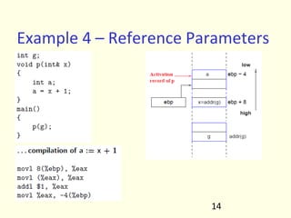
- 21. 11 The big picture • Compiler is part of program development environment • The other typical components of this environment are editor, assembler, linker, loader, debugger, profiler etc. • The compiler (and all other tools) must support each other for easy program development
- 26. 12 Editor Compiler Assembler Linker Loader Programmer Source Program Assembly code Machine Code Resolved Machine Code Executable Image Execution on the target machine
- 27. 12 Editor Compiler Assembler Linker Loader Programmer Source Program Assembly code Machine Code Resolved Machine Code Executable Image Execution on the target machine Normally end up with error
- 28. 12 Editor Compiler Assembler Linker Loader Debugger Programmer Source Program Assembly code Machine Code Resolved Machine Code Executable Image Debugging results Execution on the target machine Normally end up with error Execute under Control of debugger
- 29. 12 Editor Compiler Assembler Linker Loader Debugger Programmer Source Program Assembly code Machine Code Resolved Machine Code Executable Image Debugging results Programmer does manual correction of the code Execution on the target machine Normally end up with error Execute under Control of debugger
- 30. What are Compilers? • Translates from one representation of the program to another • Typically from high level source code to low level machine code or object code • Source code is normally optimized for human readability – Expressive: matches our notion of languages (and application?!) – Redundant to help avoid programming errors • Machine code is optimized for hardware – Redundancy is reduced – Information about the intent is lost 1
- 31. 2 Compiler as a Translator Compiler High level program Low level code
- 32. Goals of translation • Good compile time performance • Good performance for the generated code • Correctness – A very important issue. –Can compilers be proven to be correct? • Tedious even for toy compilers! Undecidable in general. –However, the correctness has an implication on the development cost 3
- 33. How to translate? • Direct translation is difficult. Why? • Source code and machine code mismatch in level of abstraction – Variables vs Memory locations/registers – Functions vs jump/return – Parameter passing – structs • Some languages are farther from machine code than others – For example, languages supporting Object Oriented Paradigm 4
- 34. How to translate easily? • Translate in steps. Each step handles a reasonably simple, logical, and well defined task • Design a series of program representations • Intermediate representations should be amenable to program manipulation of various kinds (type checking, optimization, code generation etc.) • Representations become more machine specific and less language specific as the translation proceeds 5
- 35. The first few steps • The first few steps can be understood by analogies to how humans comprehend a natural language • The first step is recognizing/knowing alphabets of a language. For example –English text consists of lower and upper case alphabets, digits, punctuations and white spaces –Written programs consist of characters from the ASCII characters set (normally 9-13, 32-126) 6
- 36. The first few steps • The next step to understand the sentence is recognizing words –How to recognize English words? –Words found in standard dictionaries –Dictionaries are updated regularly 7
- 37. The first few steps • How to recognize words in a programming language? –a dictionary (of keywords etc.) –rules for constructing words (identifiers, numbers etc.) • This is called lexical analysis • Recognizing words is not completely trivial. For example: w hat ist his se nte nce? 8
- 38. Lexical Analysis: Challenges • We must know what the word separators are • The language must define rules for breaking a sentence into a sequence of words. • Normally white spaces and punctuations are word separators in languages. 9
- 39. Lexical Analysis: Challenges • In programming languages a character from a different class may also be treated as word separator. • The lexical analyzer breaks a sentence into a sequence of words or tokens: –If a == b then a = 1 ; else a = 2 ; –Sequence of words (total 14 words) if a == b then a = 1 ; else a = 2 ; 10
- 40. The next step • Once the words are understood, the next step is to understand the structure of the sentence • The process is known as syntax checking or parsing I am going to play pronoun aux verb adverb subject verb adverb-phrase Sentence 11
- 41. Parsing • Parsing a program is exactly the same process as shown in previous slide. • Consider an expression if x == y then z = 1 else z = 2 if stmt predicate then-stmt else-stmt = = = = x y z 1 z 2 12
- 42. Understanding the meaning • Once the sentence structure is understood we try to understand the meaning of the sentence (semantic analysis) • A challenging task • Example: Prateek said Nitin left his assignment at home • What does his refer to? Prateek or Nitin? 13
- 43. Understanding the meaning • Worse case Amit said Amit left his assignment at home • Even worse Amit said Amit left Amit’s assignment at home • How many Amits are there? Which one left the assignment? Whose assignment got left? 14
- 44. Semantic Analysis • Too hard for compilers. They do not have capabilities similar to human understanding • However, compilers do perform analysis to understand the meaning and catch inconsistencies • Programming languages define strict rules to avoid such ambiguities { int Amit = 3; { int Amit = 4; cout << Amit; } } 15
- 45. More on Semantic Analysis • Compilers perform many other checks besides variable bindings • Type checking Amit left her work at home • There is a type mismatch between her and Amit. Presumably Amit is a male. And they are not the same person. 16
- 46. अश्वथामा हत: इतत नरो वा क ु ञ्जरो वा “Ashwathama hathaha iti, narova kunjarova” Ashwathama is dead. But, I am not certain whether it was a human or an elephant Example from Mahabharat
- 47. Compiler structure once again 18 Compiler Front End Lexical Analysis Syntax Analysis Semantic Analysis (Language specific) Token stream Abstract Syntax tree Unambiguous Program representation Source Program Target Program Back End
- 49. Code Optimization • No strong counter part with English, but is similar to editing/précis writing • Automatically modify programs so that they –Run faster –Use less resources (memory, registers, space, fewer fetches etc.) 23
- 50. Code Optimization • Some common optimizations –Common sub-expression elimination –Copy propagation –Dead code elimination –Code motion –Strength reduction –Constant folding • Example: x = 15 * 3 is transformed to x = 45 24
- 51. Example of Optimizations A : assignment M : multiplication D : division E : exponent PI = 3.14159 Area = 4 * PI * R^2 Volume = (4/3) * PI * R^3 3A+4M+1D+2E -------------------------------- X = 3.14159 * R * R Area = 4 * X Volume = 1.33 * X * R 3A+5M -------------------------------- Area = 4 * 3.14159 * R * R Volume = ( Area / 3 ) * R 2A+4M+1D -------------------------------- Area = 12.56636 * R * R Volume = ( Area /3 ) * R 2A+3M+1D -------------------------------- X = R * R Area = 12.56636 * X Volume = 4.18879 * X * R 3A+4M 25
- 52. Code Generation • Usually a two step process –Generate intermediate code from the semantic representation of the program –Generate machine code from the intermediate code • The advantage is that each phase is simple • Requires design of intermediate language 26
- 53. Code Generation • Most compilers perform translation between successive intermediate representations • Intermediate languages are generally ordered in decreasing level of abstraction from highest (source) to lowest (machine) 27
- 54. Code Generation • Abstractions at the source level identifiers, operators, expressions, statements, conditionals, iteration, functions (user defined, system defined or libraries) • Abstraction at the target level memory locations, registers, stack, opcodes, addressing modes, system libraries, interface to the operating systems • Code generation is mapping from source level abstractions to target machine abstractions 28
- 55. Code Generation • Map identifiers to locations (memory/storage allocation) • Explicate variable accesses (change identifier reference to relocatable/absolute address • Map source operators to opcodes or a sequence of opcodes 29
- 56. Code Generation • Convert conditionals and iterations to a test/jump or compare instructions • Layout parameter passing protocols: locations for parameters, return values, layout of activations frame etc. • Interface calls to library, runtime system, operating systems 30
- 57. Post translation Optimizations • Algebraic transformations and reordering –Remove/simplify operations like • Multiplication by 1 • Multiplication by 0 • Addition with 0 –Reorder instructions based on • Commutative properties of operators • For example x+y is same as y+x (always?) 31
- 58. Post translation Optimizations Instruction selection –Addressing mode selection –Opcode selection –Peephole optimization 32
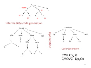
- 59. 33 if == = b 0 a b boolean int int int int int ; Intermediate code generation Optimization Code Generation CMP Cx, 0 CMOVZ Dx,Cx
- 60. Compiler structure 34 Compiler Front End Lexical Analysis Syntax Analysis Semantic Analysis (Language specific) Token stream Abstract Syntax tree Unambiguous Program representation Source Program Target Program Optimizer Optimized code Optional Phase IL code generator IL code Code generator Back End Machine specific
- 61. Something is missing • Information required about the program variables during compilation – Class of variable: keyword, identifier etc. – Type of variable: integer, float, array, function etc. – Amount of storage required – Address in the memory – Scope information • Location to store this information – Attributes with the variable (has obvious problems) – At a central repository and every phase refers to the repository whenever information is required • Normally the second approach is preferred – Use a data structure called symbol table 35
- 62. Final Compiler structure 36 Compiler Front End Lexical Analysis Syntax Analysis Semantic Analysis (Language specific) Token stream Abstract Syntax tree Unambiguous Program representation Source Program Target Program Optimizer Optimized code Optional Phase IL code generator IL code Code generator Back End Machine specific Symbol Table
- 63. Advantages of the model • Also known as Analysis-Synthesis model of compilation – Front end phases are known as analysis phases – Back end phases are known as synthesis phases • Each phase has a well defined work • Each phase handles a logical activity in the process of compilation 37
- 64. Advantages of the model … • Compiler is re-targetable • Source and machine independent code optimization is possible. • Optimization phase can be inserted after the front and back end phases have been developed and deployed 38
- 65. Issues in Compiler Design • Compilation appears to be very simple, but there are many pitfalls • How are erroneous programs handled? • Design of programming languages has a big impact on the complexity of the compiler • M*N vs. M+N problem – Compilers are required for all the languages and all the machines – For M languages and N machines we need to develop M*N compilers – However, there is lot of repetition of work because of similar activities in the front ends and back ends – Can we design only M front ends and N back ends, and some how link them to get all M*N compilers? 39
- 66. M*N vs M+N Problem 40 F1 F2 F3 FM B1 B2 B3 BN Requires M*N compilers F1 F2 F3 FM B1 B2 B3 BN Intermediate Language IL Requires M front ends And N back ends
- 67. Universal Intermediate Language • Impossible to design a single intermediate language to accommodate all programming languages – Mythical universal intermediate language sought since mid 1950s (Aho, Sethi, Ullman) • However, common IRs for similar languages, and similar machines have been designed, and are used for compiler development 41
- 68. How do we know compilers generate correct code? • Prove that the compiler is correct. • However, program proving techniques do not exist at a level where large and complex programs like compilers can be proven to be correct • In practice do a systematic testing to increase confidence level 42
- 69. • Regression testing – Maintain a suite of test programs – Expected behavior of each program is documented – All the test programs are compiled using the compiler and deviations are reported to the compiler writer • Design of test suite – Test programs should exercise every statement of the compiler at least once – Usually requires great ingenuity to design such a test suite – Exhaustive test suites have been constructed for some languages 43
- 70. How to reduce development and testing effort? • DO NOT WRITE COMPILERS • GENERATE compilers • A compiler generator should be able to “generate” compiler from the source language and target machine specifications 44 Compiler Compiler Generator Source Language Specification Target Machine Specification
- 71. Tool based Compiler Development 45 Lexical Analyzer Parser Semantic Analyzer Optimizer IL code generator Code generator Source Program Target Program Lexical Analyzer Generator Lexeme specs Parser Generator Parser specs Other phase Generators Phase Specifications Code Generator generator Machine specifications
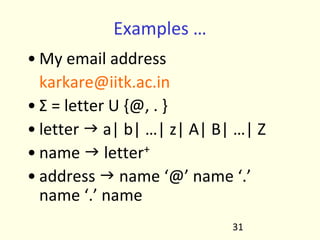
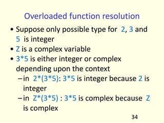
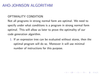
- 72. Bootstrapping • Compiler is a complex program and should not be written in assembly language • How to write compiler for a language in the same language (first time!)? • First time this experiment was done for Lisp • Initially, Lisp was used as a notation for writing functions. • Functions were then hand translated into assembly language and executed • McCarthy wrote a function eval[e] in Lisp that took a Lisp expression e as an argument • The function was later hand translated and it became an interpreter for Lisp 46
- 73. Bootstrap Image By: No machine-readable author provided. Tarquin~commonswiki assumed (based on copyright claims). - No machine-readable source provided. Own work assumed (based on copyright claims)., CC BY-SA 3.0, https://commons.wikimedia.org/w/index.php?curid=105468
- 74. Bootstrapping: Example • Lets solve a simpler problem first • Existing architecture and C compiler: –gcc-x86 compiles C language to x86 • New architecture: –x335 • How to develop cc-x335? –runs on x335, generates code for x335 48
- 75. Bootstrapping: Example • How to develop cc-x335? • Write a C compiler in C that emits x335 code • Compile using gcc-x86 on x86 machine • We have a C compiler that emits x335 code –But runs on x86, not x355 / 49
- 76. Bootstrapping: Example • We have cc-x86-x335 • Compiler runs on x86, generated code runs on x355 • Compile the source code of C compiler with cc-x86-x335 • There it is • the output is a binary that runs on x335 • this binary is the desired compiler : cc-x335
- 77. Bootstrapping … • A compiler can be characterized by three languages: the source language (S), the target language (T), and the implementation language (I) • The three language S, I, and T can be quite different. Such a compiler is called cross-compiler • This is represented by a T-diagram as: • In textual form this can be represented as SIT 51 S T I
- 78. • Write a cross compiler for a language L in implementation language S to generate code for machine N • Existing compiler for S runs on a different machine M and generates code for M • When Compiler LSN is run through SMM we get compiler LMN 52 S M M L S N L M N C PDP11 PDP11 EQN TROFF C EQN TROFF PDP11
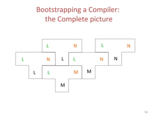
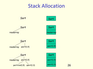
- 79. Bootstrapping a Compiler • Suppose LNN is to be developed on a machine M where LMM is available • Compile LLN second time using the generated compiler 53 L M M L L N L M N L L N L M N L N N
- 80. 54 L N L L L L L L N M M M N N N Bootstrapping a Compiler: the Complete picture
- 81. Compilers of the 21st Century • Overall structure of almost all the compilers is similar to the structure we have discussed • The proportions of the effort have changed since the early days of compilation • Earlier front end phases were the most complex and expensive parts. • Today back end phases and optimization dominate all other phases. Front end phases are typically a smaller fraction of the total time 55
- 82. Lexical Analysis • Recognize tokens and ignore white spaces, comments • Error reporting • Model using regular expressions • Recognize using Finite State Automata1 Generates token stream
- 83. Lexical Analysis • Sentences consist of string of tokens (a syntactic category) For example, number, identifier, keyword, string • Sequences of characters in a token is a lexeme for example, 100.01, counter, const, “How are you?” • Rule of description is a pattern for example, letter ( letter | digit )* • Task: Identify Tokens and corresponding Lexemes 2
- 84. Lexical Analysis • Examples • Construct constants: for example, convert a number to token num and pass the value as its attribute, – 31 becomes <num, 31> • Recognize keyword and identifiers – counter = counter + increment becomes id = id + id – check that id here is not a keyword • Discard whatever does not contribute to parsing – white spaces (blanks, tabs, newlines) and comments 3
- 85. Interface to other phases • Why do we need Push back? • Required due to look-ahead for example, to recognize >= and > • Typically implemented through a buffer – Keep input in a buffer – Move pointers over the input 4 Lexical Analyzer Syntax Analyzer Input Ask for token Token Read characters Push back Extra characters
- 86. Approaches to implementation • Use assembly language Most efficient but most difficult to implement • Use high level languages like C Efficient but difficult to implement • Use tools like lex, flex Easy to implement but not as efficient as the first two cases 5
- 87. Symbol Table • Stores information for subsequent phases • Interface to the symbol table –Insert(s,t): save lexeme s and token t and return pointer –Lookup(s): return index of entry for lexeme s or 0 if s is not found 9
- 88. Implementation of Symbol Table • Fixed amount of space to store lexemes. –Not advisable as it waste space. • Store lexemes in a separate array. –Each lexeme is separated by eos. –Symbol table has pointers to lexemes. 10
- 89. Fixed space for lexemes Other attributes Usually 32 bytes lexeme1 lexeme2 eos eos lexeme3 …… Other attributes Usually 4 bytes 11
- 90. How to handle keywords? • Consider token DIV and MOD with lexemes div and mod. • Initialize symbol table with insert( “div” , DIV ) and insert( “mod” , MOD). • Any subsequent insert fails (unguarded insert) • Any subsequent lookup returns the keyword value, therefore, these cannot be used as an identifier. 12
- 91. Difficulties in the design of lexical analyzers 13 Is it as simple as it sounds?
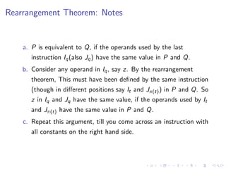
- 92. Lexical analyzer: Challenges • Lexemes in a fixed position. Fixed format vs. free format languages • FORTRAN Fixed Format – 80 columns per line – Column 1-5 for the statement number/label column – Column 6 for continuation mark (?) – Column 7-72 for the program statements – Column 73-80 Ignored (Used for other purpose) – Letter C in Column 1 meant the current line is a comment 14
- 93. Lexical analyzer: Challenges • Handling of blanks – in C, blanks separate identifiers – in FORTRAN, blanks are important only in literal strings – variable counter is same as count er – Another example DO 10 I = 1.25 DO 10 I = 1,25 15 DO10I=1.25 DO10I=1,25
- 94. • The first line is a variable assignment DO10I=1.25 • The second line is beginning of a Do loop • Reading from left to right one can not distinguish between the two until the “;” or “.” is reached 16
- 95. 17 Fortran white space and fixed format rules came into force due to punch cards and errors in punching
- 96. 18 Fortran white space and fixed format rules came into force due to punch cards and errors in punching
- 97. PL/1 Problems • Keywords are not reserved in PL/1 if then then then = else else else = then if if then then = then + 1 • PL/1 declarations Declare(arg1,arg2,arg3,…….,argn) • Cannot tell whether Declare is a keyword or array reference until after “)” • Requires arbitrary lookahead and very large buffers. – Worse, the buffers may have to be reloaded. 19
- 98. Problem continues even today!! • C++ template syntax: Foo<Bar> • C++ stream syntax: cin >> var; • Nested templates: Foo<Bar<Bazz>> • Can these problems be resolved by lexical analyzers alone? 20
- 99. How to specify tokens? • How to describe tokens 2.e0 20.e-01 2.000 • How to break text into token if (x==0) a = x << 1; if (x==0) a = x < 1; • How to break input into tokens efficiently – Tokens may have similar prefixes – Each character should be looked at only once 21
- 100. How to describe tokens? • Programming language tokens can be described by regular languages • Regular languages – Are easy to understand – There is a well understood and useful theory – They have efficient implementation • Regular languages have been discussed in great detail in the “Theory of Computation” course 22
- 101. How to specify tokens • Regular definitions – Let ri be a regular expression and di be a distinct name – Regular definition is a sequence of definitions of the form d1 J r1 d2 J r2 ….. dn J rn – Where each ri is a regular expression over Σ U {d1, d2, …, di-1} 29
- 102. Examples • My fax number 91-(512)-259-7586 • Σ = digit U {-, (, ) } • Country J digit+ • Area J ‘(‘ digit+ ‘)’ • Exchange J digit+ • Phone J digit+ • Number J country ‘-’ area ‘-’ exchange ‘-’ phone 30 digit2 digit3 digit3 digit4
- 103. Examples … • My email address [email protected] • Σ = letter U {@, . } • letter J a| b| …| z| A| B| …| Z • name J letter+ • address J name ‘@’ name ‘.’ name ‘.’ name 31
- 104. Examples … • Identifier letter J a| b| …|z| A| B| …| Z digit J 0| 1| …| 9 identifier J letter(letter|digit)* • Unsigned number in C digit J 0| 1| …|9 digits J digit+ fraction J ’.’ digits | є exponent J (E ( ‘+’ | ‘-’ | є) digits) | є number J digits fraction exponent 32
- 105. Regular expressions in specifications • Regular expressions describe many useful languages • Regular expressions are only specifications; implementation is still required • Given a string s and a regular expression R, does s Є L(R) ? • Solution to this problem is the basis of the lexical analyzers • However, just the yes/no answer is not sufficient • Goal: Partition the input into tokens 33
- 106. 1. Write a regular expression for lexemes of each token • number Æ digit+ • identifier Æ letter(letter|digit)+ 2. Construct R matching all lexemes of all tokens • R = R1 + R2 + R3 + ….. 3. Let input be x1…xn • for 1 ≤ i ≤ n check x1…xi Є L(R) 4. x1…xi Є L(R) B x1…xi Є L(Rj) for some j • smallest such j is token class of x1…xi 5. Remove x1…xi from input; go to (3) 34
- 107. • The algorithm gives priority to tokens listed earlier – Treats “if” as keyword and not identifier • How much input is used? What if – x1…xi Є L(R) – x1…xj Є L(R) – Pick up the longest possible string in L(R) – The principle of “maximal munch” • Regular expressions provide a concise and useful notation for string patterns • Good algorithms require a single pass over the input 35
- 108. How to break up text • Elsex=0 • Regular expressions alone are not enough • Normally the longest match wins • Ties are resolved by prioritizing tokens • Lexical definitions consist of regular definitions, priority rules and maximal munch principle 36 else x = 0 elsex = 0
- 109. Transition Diagrams • Regular expression are declarative specifications • Transition diagram is an implementation • A transition diagram consists of – An input alphabet belonging to Σ – A set of states S – A set of transitions statei →𝑖𝑛𝑝𝑢𝑡 statej – A set of final states F – A start state n • Transition s1 →𝑎 s2 is read: in state s1 on input 𝑎 go to state s2 • If end of input is reached in a final state then accept • Otherwise, reject 37
- 110. Pictorial notation • A state • A final state • Transition • Transition from state i to state j on an input a 38 i j a
- 111. How to recognize tokens • Consider relop Æ < | <= | = | <> | >= | > id Æ letter(letter|digit)* num Æ digit+ (‘.’ digit+)? (E(‘+’|’-’)? digit+)? delim Æ blank | tab | newline ws Æ delim+ • Construct an analyzer that will return <token, attribute> pairs 39
- 112. Transition diagram for relops > = other token is relop, lexeme is >= token is relop, lexeme is > * < > > = = = other other * * token is relop, lexeme is >= token is relop, lexeme is > token is relop, lexeme is < token is relop, lexeme is <> token is relop, lexeme is <= token is relop, lexeme is = 40
- 113. Transition diagram for identifier letter digit other delim letter other delim * * Transition diagram for white spaces 41
- 114. digit digit digit others * Transition diagram for unsigned numbers digit digit digit others * . digit digit digit digit digit digit digit . E E others * + - Integer number Real numbers 42
- 115. • The lexeme for a given token must be the longest possible • Assume input to be 12.34E56 • Starting in the third diagram the accept state will be reached after 12 • Therefore, the matching should always start with the first transition diagram • If failure occurs in one transition diagram then retract the forward pointer to the start state and activate the next diagram • If failure occurs in all diagrams then a lexical error has occurred 43
- 116. Implementation of transition diagrams Token nexttoken() { while(1) { switch (state) { …… case 10: c=nextchar(); if(isletter(c)) state=10; elseif (isdigit(c)) state=10; else state=11; break; …… } } } 44
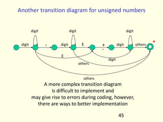
- 117. Another transition diagram for unsigned numbers digit digit digit digit digit digit digit . E E others * + - others others A more complex transition diagram is difficult to implement and may give rise to errors during coding, however, there are ways to better implementation 45
- 118. Lexical analyzer generator • Input to the generator – List of regular expressions in priority order – Associated actions for each of regular expression (generates kind of token and other book keeping information) • Output of the generator – Program that reads input character stream and breaks that into tokens – Reports lexical errors (unexpected characters), if any 46
- 119. LEX: A lexical analyzer generator 47 LEX C Compiler Lexical analyzer Token specifications lex.yy.c C code for Lexical analyzer Object code Input program tokens Refer to LEX User’s Manual
- 120. How does LEX work? • Regular expressions describe the languages that can be recognized by finite automata • Translate each token regular expression into a non deterministic finite automaton (NFA) • Convert the NFA into an equivalent DFA • Minimize the DFA to reduce number of states • Emit code driven by the DFA tables 48
- 121. Syntax Analysis • Check syntax and construct abstract syntax tree • Error reporting and recovery • Model using context free grammars • Recognize using Push down automata/Table Driven Parsers 1 if == = ; b 0 a b
- 122. Limitations of regular languages • How to describe language syntax precisely and conveniently. Can regular expressions be used? • Many languages are not regular, for example, string of balanced parentheses – ((((…)))) – { (i)i | i ≥ 0 } – There is no regular expression for this language • A finite automata may repeat states, however, it cannot remember the number of times it has been to a particular state • A more powerful language is needed to describe a valid string of tokens 2
- 123. Syntax definition • Context free grammars <T, N, P, S> – T: a set of tokens (terminal symbols) – N: a set of non terminal symbols – P: a set of productions of the form nonterminal →String of terminals & non terminals – S: a start symbol • A grammar derives strings by beginning with a start symbol and repeatedly replacing a non terminal by the right hand side of a production for that non terminal. • The strings that can be derived from the start symbol of a grammar G form the language L(G) defined by the grammar. 3
- 124. Examples • String of balanced parentheses S → ( S ) S | Є • Grammar list → list + digit | list – digit | digit digit → 0 | 1 | … | 9 Consists of the language which is a list of digit separated by + or -. 4
- 125. Derivation list Î list + digit Î list – digit + digit Î digit – digit + digit Î 9 – digit + digit Î 9 – 5 + digit Î 9 – 5 + 2 Therefore, the string 9-5+2 belongs to the language specified by the grammar The name context free comes from the fact that use of a production X Æ … does not depend on the context of X 5
- 126. Examples … • Simplified Grammar for C block block Æ ‘{‘ decls statements ‘}’ statements Æ stmt-list | Є stmt–list Æ stmt-list stmt ‘;’ | stmt ‘;’ decls Æ decls declaration | Є declaration Æ … 6
- 127. Syntax analyzers • Testing for membership whether w belongs to L(G) is just a “yes” or “no” answer • However the syntax analyzer – Must generate the parse tree – Handle errors gracefully if string is not in the language • Form of the grammar is important – Many grammars generate the same language – Tools are sensitive to the grammar 7
- 128. What syntax analysis cannot do! • To check whether variables are of types on which operations are allowed • To check whether a variable has been declared before use • To check whether a variable has been initialized • These issues will be handled in semantic analysis 8
- 129. Derivation • If there is a production A Æ α then we say that A derives α and is denoted by A B α • α A β B α γ β if A Æ γ is a production • If α1 B α2 B … B αn then α1 B αn • Given a grammar G and a string w of terminals in L(G) we can write S B w • If S B α where α is a string of terminals and non terminals of G then we say that α is a sentential form of G 9 + + *
- 130. Derivation … • If in a sentential form only the leftmost non terminal is replaced then it becomes leftmost derivation • Every leftmost step can be written as wAγ Blm* wδγ where w is a string of terminals and A Æ δ is a production • Similarly, right most derivation can be defined • An ambiguous grammar is one that produces more than one leftmost (rightmost) derivation of a sentence 10
- 131. Parse tree • shows how the start symbol of a grammar derives a string in the language • root is labeled by the start symbol • leaf nodes are labeled by tokens • Each internal node is labeled by a non terminal • if A is the label of anode and x1, x2, …xn are labels of the children of that node then A Æ x1 x2 … xn is a production in the grammar 11
- 132. Example Parse tree for 9-5+2 12 list list list digit digit + - digit 9 5 2
- 133. Ambiguity • A Grammar can have more than one parse tree for a string • Consider grammar list Æ list+ list | list – list | 0 | 1 | … | 9 • String 9-5+2 has two parse trees 13
- 134. 14 list + list - list list 9 list 2 5 list list - list 9 list + list 5 2
- 135. Ambiguity … • Ambiguity is problematic because meaning of the programs can be incorrect • Ambiguity can be handled in several ways – Enforce associativity and precedence – Rewrite the grammar (cleanest way) • There is no algorithm to convert automatically any ambiguous grammar to an unambiguous grammar accepting the same language • Worse, there are inherently ambiguous languages! 15
- 136. Ambiguity in Programming Lang. • Dangling else problem stmt o if expr stmt | if expr stmt else stmt • For this grammar, the string if e1 if e2 then s1 else s2 has two parse trees 16
- 137. 17 stmt if expr stmt else stmt expr stmt if e1 s2 e2 s1 stmt if expr stmt stmt else stmt expr if e1 e2 s1 s2 if e1 if e2 s1 else s2 if e1 if e2 s1 else s2
- 138. Resolving dangling else problem • General rule: match each else with the closest previous unmatched if. The grammar can be rewritten as stmt o matched-stmt | unmatched-stmt matched-stmt o if expr matched-stmt else matched-stmt | others unmatched-stmt o if expr stmt | if expr matched-stmt else unmatched-stmt 18
- 139. Associativity • If an operand has operator on both the sides, the side on which operator takes this operand is the associativity of that operator • In a+b+c b is taken by left + • +, -, *, / are left associative • ^, = are right associative • Grammar to generate strings with right associative operators right Æ letter = right | letter letter Æ a| b |…| z 19
- 140. Precedence • String a+5*2 has two possible interpretations because of two different parse trees corresponding to (a+5)*2 and a+(5*2) • Precedence determines the correct interpretation. • Next, an example of how precedence rules are encoded in a grammar 20
- 141. Precedence/Associativity in the Grammar for Arithmetic Expressions Ambiguous E Æ E + E | E * E | (E) | num | id 3 + 2 + 5 3 + 2 * 5 21 • Unambiguous, with precedence and associativity rules honored E Æ E + T | T T Æ T * F | F F Æ ( E ) | num | id
- 142. Parsing • Process of determination whether a string can be generated by a grammar • Parsing falls in two categories: – Top-down parsing: Construction of the parse tree starts at the root (from the start symbol) and proceeds towards leaves (token or terminals) – Bottom-up parsing: Construction of the parse tree starts from the leaf nodes (tokens or terminals of the grammar) and proceeds towards root (start symbol) 22
- 143. Top down Parsing • Following grammar generates types of Pascal type Æ simple | n id | array [ simple] of type simple Æ integer | char | num dotdot num 1
- 144. Example … • Construction of a parse tree is done by starting the root labeled by a start symbol • repeat following two steps – at a node labeled with non terminal A select one of the productions of A and construct children nodes – find the next node at which subtree is Constructed 2 (Which production?) (Which node?)
- 145. • Parse array [ num dotdot num ] of integer • Cannot proceed as non terminal “simple” never generates a string beginning with token “array”. Therefore, requires back-tracking. • Back-tracking is not desirable, therefore, take help of a “look-ahead” token. The current token is treated as look- ahead token. (restricts the class of grammars) 3 type simple Start symbol Expanded using the rule type Æ simple
- 146. 4 array [ num dotdot num ] of integer type simple ] type [ array dotdot num num simple integer look-ahead of Start symbol Expand using the rule type Æ array [ simple ] of type Left most non terminal Expand using the rule Simple Æ num dotdot num Left most non terminal Expand using the rule type Æ simple Left most non terminal Expand using the rule simple Æ integer all the tokens exhausted Parsing completed
- 147. Recursive descent parsing First set: Let there be a production A o D then First(D) is the set of tokens that appear as the first token in the strings generated from D For example : First(simple) = {integer, char, num} First(num dotdot num) = {num} 5
- 148. Define a procedure for each non terminal procedure type; if lookahead in {integer, char, num} then simple else if lookahead = n then begin match( n ); match(id) end else if lookahead = array then begin match(array); match([); simple; match(]); match(of); type end else error; 6
- 149. procedure simple; if lookahead = integer then match(integer) else if lookahead = char then match(char) else if lookahead = num then begin match(num); match(dotdot); match(num) end else error; procedure match(t:token); if lookahead = t then lookahead = next token else error; 7
- 150. Left recursion • A top down parser with production A o A D may loop forever • From the grammar A o A D | E left recursion may be eliminated by transforming the grammar to A o E R R o D R | H 8
- 151. 9 A A A β α α A R R β α Є Parse tree corresponding to a left recursive grammar Parse tree corresponding to the modified grammar Both the trees generate string βα*
- 152. Example • Consider grammar for arithmetic expressions E Æ E + T | T T Æ T * F | F F Æ ( E ) | id • After removal of left recursion the grammar becomes E Æ T E’ E’ Æ + T E’ | Є T Æ F T’ T’ Æ* F T’ | Є F Æ ( E ) | id 10
- 153. Removal of left recursion In general A Æ AD1 | AD2 | ….. |ADm |E1 | E2 | …… | En transforms to A Æ E1A' | E2A' | …..| EnA' A' Æ D1A' | D2A' |…..| DmA' | Є 11
- 154. Left recursion hidden due to many productions • Left recursion may also be introduced by two or more grammar rules. For example: S Æ Aa | b A Æ Ac | Sd | Є there is a left recursion because S o Aa o Sda • In such cases, left recursion is removed systematically – Starting from the first rule and replacing all the occurrences of the first non terminal symbol – Removing left recursion from the modified grammar 12
- 155. Removal of left recursion due to many productions … • After the first step (substitute S by its rhs in the rules) the grammar becomes S Æ Aa | b A Æ Ac | Aad | bd | Є • After the second step (removal of left recursion) the grammar becomes S Æ Aa | b A Æ bdA' | A' A' Æ cA' | adA' | Є 13
- 156. Left factoring • In top-down parsing when it is not clear which production to choose for expansion of a symbol defer the decision till we have seen enough input. In general if A Æ DE1 | DE2 defer decision by expanding A to DA' we can then expand A’ to E1 or E2 • Therefore A Æ D E1 | D E2 transforms to A Æ DA’ A’ Æ E1 | E2 14
- 157. Dangling else problem again Dangling else problem can be handled by left factoring stmt Æ if expr then stmt else stmt | if expr then stmt can be transformed to stmt Æ if expr then stmt S' S' Æ else stmt | Є 15
- 158. Predictive parsers • A non recursive top down parsing method • Parser “predicts” which production to use • It removes backtracking by fixing one production for every non-terminal and input token(s) • Predictive parsers accept LL(k) languages – First L stands for left to right scan of input – Second L stands for leftmost derivation – k stands for number of lookahead token • In practice LL(1) is used 16
- 159. Predictive parsing • Predictive parser can be implemented by maintaining an external stack 17 input stack parser Parse table output Parse table is a two dimensional array M*X,a+ where “X” is a non terminal and “a” is a terminal of the grammar
- 160. Example • Consider the grammar E Æ T E’ E' Æ +T E' | Є T Æ F T' T' Æ * F T' | Є F Æ ( E ) | id 18
- 161. Parse table for the grammar id + * ( ) $ E EÆTE’ EÆTE’ E’ E’Æ+TE’ E’ÆЄ E’ÆЄ T TÆFT’ TÆFT’ T’ T’ÆЄ T’Æ*FT’ T’ÆЄ T’ÆЄ F FÆid FÆ(E) 19 Blank entries are error states. For example E cannot derive a string starting with ‘+’
- 162. Parsing algorithm • The parser considers 'X' the symbol on top of stack, and 'a' the current input symbol • These two symbols determine the action to be taken by the parser • Assume that '$' is a special token that is at the bottom of the stack and terminates the input string if X = a = $ then halt if X = a ≠ $ then pop(x) and ip++ if X is a non terminal then if M[X,a] = {X Æ UVW} then begin pop(X); push(W,V,U) end else error 20
- 163. Example Stack input action $E id + id * id $ expand by EÆTE’ $E’T id + id * id $ expand by TÆFT’ $E’T’F id + id * id $ expand by FÆid $E’T’id id + id * id $ pop id and ip++ $E’T’ + id * id $ expand by T’ÆЄ $E’ + id * id $ expand by E’Æ+TE’ $E’T+ + id * id $ pop + and ip++ $E’T id * id $ expand by TÆFT’ 21
- 164. Example … Stack input action $E’T’F id * id $ expand by FÆid $E’T’id id * id $ pop id and ip++ $E’T’ * id $ expand by T’Æ*FT’ $E’T’F* * id $ pop * and ip++ $E’T’F id $ expand by FÆid $E’T’id id $ pop id and ip++ $E’T’ $ expand by T’ÆЄ $E’ $ expand by E’ÆЄ $ $ halt 22
- 165. Constructing parse table • Table can be constructed if for every non terminal, every lookahead symbol can be handled by at most one production • First(α) for a string of terminals and non terminals α is – Set of symbols that might begin the fully expanded (made of only tokens) version of α • Follow(X) for a non terminal X is – set of symbols that might follow the derivation of X in the input stream 23 first follow X
- 166. Compute first sets • If X is a terminal symbol then First(X) = {X} • If X Æ Є is a production then Є is in First(X) • If X is a non terminal and X Æ YlY2 … Yk is a production then if for some i, a is in First(Yi) and Є is in all of First(Yj) (such that j<i) then a is in First(X) • If Є is in First (Y1) … First(Yk) then Є is in First(X) 24
- 167. Example • For the expression grammar E Æ T E’ E' Æ +T E' | Є T Æ F T' T' Æ * F T' | Є F Æ ( E ) | id First(E) = First(T) = First(F) = { (, id } First(E') = {+, Є} First(T') = { *, Є} 25
- 168. Compute follow sets 1. Place $ in follow(S) 2. If there is a production A → αBβ then everything in first(β) (except ε) is in follow(B) 3. If there is a production A → αB then everything in follow(A) is in follow(B) 4. If there is a production A → αBβ and First(β) contains ε then everything in follow(A) is in follow(B) Since follow sets are defined in terms of follow sets last two steps have to be repeated until follow sets converge 26
- 169. Example • For the expression grammar E Æ T E’ E' Æ + T E' | Є T Æ F T' T' Æ * F T' | Є F Æ ( E ) | id follow(E) = follow(E’) = , $, ) - follow(T) = follow(T’) = , $, ), + - follow(F) = { $, ), +, *} 27
- 170. Construction of parse table • for each production A Æ α do – for each terminal ‘a’ in first(α) M[A,a] = A Æ α – If Є is in First(α) M[A,b] = A Æ α for each terminal b in follow(A) – If ε is in First(α) and $ is in follow(A) M[A,$] = A Æ α • A grammar whose parse table has no multiple entries is called LL(1) 28
- 171. Practice Assignment • Construct LL(1) parse table for the expression grammar bexpr Æ bexpr or bterm | bterm bterm Æ bterm and bfactor | bfactor bfactor Æ not bfactor | ( bexpr ) | true | false • Steps to be followed – Remove left recursion – Compute first sets – Compute follow sets – Construct the parse table 29
- 172. Error handling • Stop at the first error and print a message – Compiler writer friendly – But not user friendly • Every reasonable compiler must recover from errors and identify as many errors as possible • However, multiple error messages due to a single fault must be avoided • Error recovery methods – Panic mode – Phrase level recovery – Error productions – Global correction 30
- 173. Panic mode • Simplest and the most popular method • Most tools provide for specifying panic mode recovery in the grammar • When an error is detected – Discard tokens one at a time until a set of tokens is found whose role is clear – Skip to the next token that can be placed reliably in the parse tree 31
- 174. Panic mode … • Consider following code begin a = b + c; x = p r ; h = x < 0; end; • The second expression has syntax error • Panic mode recovery for begin-end block skip ahead to next ‘;’ and try to parse the next expression • It discards one expression and tries to continue parsing • May fail if no further ‘;’ is found 32
- 175. Phrase level recovery • Make local correction to the input • Works only in limited situations – A common programming error which is easily detected – For example insert a “;” after closing “-” of a class definition • Does not work very well! 33
- 176. Error productions • Add erroneous constructs as productions in the grammar • Works only for most common mistakes which can be easily identified • Essentially makes common errors as part of the grammar • Complicates the grammar and does not work very well 34
- 177. Global corrections • Considering the program as a whole find a correct “nearby” program • Nearness may be measured using certain metric • PL/C compiler implemented this scheme: anything could be compiled! • It is complicated and not a very good idea! 35
- 178. Error Recovery in LL(1) parser • Error occurs when a parse table entry M[A,a] is empty • Skip symbols in the input until a token in a selected set (synch) appears • Place symbols in follow(A) in synch set. Skip tokens until an element in follow(A) is seen. Pop(A) and continue parsing • Add symbol in first(A) in synch set. Then it may be possible to resume parsing according to A if a symbol in first(A) appears in input. 36
- 179. Practice Assignment • Reading assignment: Read about error recovery in LL(1) parsers • Assignment to be submitted: – introduce synch symbols (using both follow and first sets) in the parse table created for the boolean expression grammar in the previous assignment – Parse “not (true and or false)” and show how error recovery works 37
- 180. 1 Bottom up parsing • Construct a parse tree for an input string beginning at leaves and going towards root OR • Reduce a string w of input to start symbol of grammar Consider a grammar S Æ aABe A Æ Abc | b B Æ d And reduction of a string a b b c d e a A b c d e a A d e a A B e S The sentential forms happen to be a right most derivation in the reverse order. S Î a A B e Î a A d e Î a A b c d e Î a b b c d e
- 181. 2 • Split string being parsed into two parts – Two parts are separated by a special character “.” – Left part is a string of terminals and non terminals – Right part is a string of terminals • Initially the input is .w Shift reduce parsing
- 182. 3 Shift reduce parsing … • Bottom up parsing has two actions • Shift: move terminal symbol from right string to left string if string before shift is α.pqr then string after shift is αp.qr
- 183. 4 Shift reduce parsing … • Reduce: immediately on the left of “.” identify a string same as RHS of a production and replace it by LHS if string before reduce action is αβ.pqr and AÆβ is a production then string after reduction is αA.pqr
- 184. 5 Example Assume grammar is E Æ E+E | E*E | id Parse id*id+id Assume an oracle tells you when to shift / when to reduce String action (by oracle) .id*id+id shift id.*id+id reduce EÆid E.*id+id shift E*.id+id shift E*id.+id reduce EÆid E*E.+id reduce EÆE*E E.+id shift E+.id shift E+id. Reduce EÆid E+E. Reduce EÆE+E E. ACCEPT
- 185. 6 Shift reduce parsing … • Symbols on the left of “.” are kept on a stack – Top of the stack is at “.” – Shift pushes a terminal on the stack – Reduce pops symbols (rhs of production) and pushes a non terminal (lhs of production) onto the stack • The most important issue: when to shift and when to reduce • Reduce action should be taken only if the result can be reduced to the start symbol
- 186. 7 Issues in bottom up parsing • How do we know which action to take –whether to shift or reduce –Which production to use for reduction? • Sometimes parser can reduce but it should not: XÆЄ can always be used for reduction!
- 187. 8 Issues in bottom up parsing • Sometimes parser can reduce in different ways! • Given stack δ and input symbol a, should the parser –Shift a onto stack (making it δa) –Reduce by some production AÆβ assuming that stack has form αβ (making it αA) –Stack can have many combinations of αβ –How to keep track of length of β?
- 188. Handles • The basic steps of a bottom-up parser are – to identify a substring within a rightmost sentential form which matches the RHS of a rule. – when this substring is replaced by the LHS of the matching rule, it must produce the previous rightmost-sentential form. • Such a substring is called a handle
- 189. 10 Handle • A handle of a right sentential form γ is – a production rule A→ β, and – an occurrence of a sub-string β in γ such that • when the occurrence of β is replaced by A in γ, we get the previous right sentential form in a rightmost derivation of γ.
- 190. 11 Handle Formally, if S Îrm* αAw Îrm αβw, then • β in the position following α, • and the corresponding production AÆ β is a handle of αβw. • The string w consists of only terminal symbols
- 191. 12 Handle • We only want to reduce handle and not any RHS • Handle pruning: If β is a handle and A Æ β is a production then replace β by A • A right most derivation in reverse can be obtained by handle pruning.
- 192. 13 Handle: Observation • Only terminal symbols can appear to the right of a handle in a rightmost sentential form. • Why?
- 193. 14 Handle: Observation Is this scenario possible: • 𝛼𝛽𝛾 is the content of the stack • 𝐴 → 𝛾 is a handle • The stack content reduces to 𝛼𝛽𝐴 • Now B → 𝛽 is the handle In other words, handle is not on top, but buried inside stack Not Possible! Why?
- 194. 15 Handles … • Consider two cases of right most derivation to understand the fact that handle appears on the top of the stack 𝑆 → 𝛼𝐴𝑧 → 𝛼𝛽𝐵𝑦𝑧 → 𝛼𝛽𝛾𝑦𝑧 𝑆 → 𝛼𝐵𝑥𝐴𝑧 → 𝛼𝐵𝑥𝑦𝑧 → 𝛼𝛾𝑥𝑦𝑧
- 195. 16 Handle always appears on the top Case I: 𝑆 → 𝛼𝐴𝑧 → 𝛼𝛽𝐵𝑦𝑧 → 𝛼𝛽𝛾𝑦𝑧 stack input action αβγ yz reduce by BÆγ αβB yz shift y αβBy z reduce by AÆ βBy αA z Case II: 𝑆 → 𝛼𝐵𝑥𝐴𝑧 → 𝛼𝐵𝑥𝑦𝑧 → 𝛼𝛾𝑥𝑦𝑧 stack input action αγ xyz reduce by BÆγ αB xyz shift x αBx yz shift y αBxy z reduce AÆy αBxA z
- 196. 17 Shift Reduce Parsers • The general shift-reduce technique is: – if there is no handle on the stack then shift – If there is a handle then reduce • Bottom up parsing is essentially the process of detecting handles and reducing them. • Different bottom-up parsers differ in the way they detect handles.
- 197. 18 Conflicts • What happens when there is a choice –What action to take in case both shift and reduce are valid? shift-reduce conflict –Which rule to use for reduction if reduction is possible by more than one rule? reduce-reduce conflict
- 198. 19 Conflicts • Conflicts come either because of ambiguous grammars or parsing method is not powerful enough
- 199. 20 Shift reduce conflict stack input action E+E *id reduce by EÆE+E E *id shift E* id shift E*id reduce by EÆid E*E reduce byEÆE*E E stack input action E+E *id shift E+E* id shift E+E*id reduce by EÆid E+E*E reduce by EÆE*E E+E reduce by EÆE+E E Consider the grammar E Æ E+E | E*E | id and the input id+id*id
- 200. 21 Reduce reduce conflict Consider the grammar M Æ R+R | R+c | R R Æ c and the input c+c Stack input action c+c shift c +c reduce by RÆc R +c shift R+ c shift R+c reduce by RÆc R+R reduce by MÆR+R M Stack input action c+c shift c +c reduce by RÆc R +c shift R+ c shift R+c reduce by MÆR+c M
- 201. 22 LR parsing • Input buffer contains the input string. • Stack contains a string of the form S0X1S1X2……XnSn where each Xi is a grammar symbol and each Si is a state. • Table contains action and goto parts. • action table is indexed by state and terminal symbols. • goto table is indexed by state and non terminal symbols. input stack parser driver Parse table action goto output
- 202. 23 Example E Æ E + T | T T Æ T * F | F F Æ ( E ) | id State id + * ( ) $ E T F 0 s5 s4 1 2 3 1 s6 acc 2 r2 s7 r2 r2 3 r4 r4 r4 r4 4 s5 s4 8 2 3 5 r6 r6 r6 r6 6 s5 s4 9 3 7 s5 s4 10 8 s6 s11 9 r1 s7 r1 r1 10 r3 r3 r3 r3 11 r5 r5 r5 r5 Consider a grammar and its parse table goto action
- 203. 24 Actions in an LR (shift reduce) parser • Assume Si is top of stack and ai is current input symbol • Action [Si,ai] can have four values 1. sj: shift ai to the stack, goto state Sj 2. rk: reduce by rule number k 3. acc: Accept 4. err: Error (empty cells in the table)
- 204. 25 Driving the LR parser Stack: S0X1S1X2…XmSm Input: aiai+1…an$ • If action[Sm,ai] = shift S Then the configuration becomes Stack: S0X1S1……XmSmaiS Input: ai+1…an$ • If action[Sm,ai] = reduce AÆβ Then the configuration becomes Stack: S0X1S1…Xm-rSm-r AS Input: aiai+1…an$ Where r = |β| and S = goto[Sm-r,A]
- 205. 26 Driving the LR parser Stack: S0X1S1X2…XmSm Input: aiai+1…an$ • If action[Sm,ai] = accept Then parsing is completed. HALT • If action[Sm,ai] = error (or empty cell) Then invoke error recovery routine.
- 206. 27 Parse id + id * id Stack Input Action 0 id+id*id$ shift 5 0 id 5 +id*id$ reduce by FÆid 0 F 3 +id*id$ reduce by TÆF 0 T 2 +id*id$ reduce by EÆT 0 E 1 +id*id$ shift 6 0 E 1 + 6 id*id$ shift 5 0 E 1 + 6 id 5 *id$ reduce by FÆid 0 E 1 + 6 F 3 *id$ reduce by TÆF 0 E 1 + 6 T 9 *id$ shift 7 0 E 1 + 6 T 9 * 7 id$ shift 5 0 E 1 + 6 T 9 * 7 id 5 $ reduce by FÆid 0 E 1 + 6 T 9 * 7 F 10 $ reduce by TÆT*F 0 E 1 + 6 T 9 $ reduce by EÆE+T 0 E 1 $ ACCEPT
- 207. 28 Configuration of a LR parser • The tuple <Stack Contents, Remaining Input> defines a configuration of a LR parser • Initially the configuration is <S0 , a0a1…an$ > • Typical final configuration on a successful parse is < S0X1Si , $>
- 208. 29 LR parsing Algorithm Initial state: Stack: S0 Input: w$ while (1) { if (action[S,a] = shift S’) { push(a); push(S’); ip++ } else if (action[S,a] = reduce AÆβ) { pop (2*|β|) symbols; push(A); push (goto*S’’,A+) (S’’ is the state at stack top after popping symbols) } else if (action[S,a] = accept) { exit } else { error }
- 209. 30 Constructing parse table Augment the grammar • G is a grammar with start symbol S • The augmented grammar G’ for G has a new start symbol S’ and an additional production S’ Æ S • When the parser reduces by this rule it will stop with accept
- 210. Production to Use for Reduction • How do we know which production to apply in a given configuration • We can guess! – May require backtracking • Keep track of “ALL” possible rules that can apply at a given point in the input string – But in general, there is no upper bound on the length of the input string – Is there a bound on number of applicable rules?
- 211. Some hands on! • 𝐸′ → 𝐸 • 𝐸 → 𝐸 + 𝑇 • 𝐸 → 𝑇 • 𝑇 → 𝑇 ∗ 𝐹 • 𝑇 → 𝐹 • 𝐹 → (𝐸) • 𝐹 → 𝑖𝑑 Strings to Parse • id + id + id + id • id * id * id * id • id * id + id * id • id * (id + id) * id
- 212. 33 Parser states • Goal is to know the valid reductions at any given point • Summarize all possible stack prefixes α as a parser state • Parser state is defined by a DFA state that reads in the stack α • Accept states of DFA are unique reductions
- 213. 34 Viable prefixes • α is a viable prefix of the grammar if – ∃w such that αw is a right sentential form – <α,w> is a configuration of the parser • As long as the parser has viable prefixes on the stack no parser error has been seen • The set of viable prefixes is a regular language • We can construct an automaton that accepts viable prefixes
- 214. 35 LR(0) items • An LR(0) item of a grammar G is a production of G with a special symbol “.” at some position of the right side • Thus production A→XYZ gives four LR(0) items A Æ .XYZ A Æ X.YZ A Æ XY.Z A Æ XYZ.
- 215. 36 LR(0) items • An item indicates how much of a production has been seen at a point in the process of parsing – Symbols on the left of “.” are already on the stacks – Symbols on the right of “.” are expected in the input
- 216. 37 Start state • Start state of DFA is an empty stack corresponding to S’Æ.S item • This means no input has been seen • The parser expects to see a string derived from S
- 217. 38 Closure of a state • Closure of a state adds items for all productions whose LHS occurs in an item in the state, just after “.” –Set of possible productions to be reduced next –Added items have “.” located at the beginning –No symbol of these items is on the stack as yet
- 218. 39 Closure operation • Let I be a set of items for a grammar G • closure(I) is a set constructed as follows: – Every item in I is in closure (I) – If A Æ α.Bβ is in closure(I) and B Æ γ is a production then B Æ .γ is in closure(I) • Intuitively A Æα.Bβ indicates that we expect a string derivable from Bβ in input • If B Æ γ is a production then we might see a string derivable from γ at this point
- 219. 40 Example For the grammar E’ Æ E E Æ E + T | T T Æ T * F | F F → ( E ) | id If I is , E’ Æ .E } then closure(I) is E’ Æ .E E Æ .E + T E Æ .T T Æ .T * F T Æ .F F Æ .id F Æ .(E)
- 220. 41 Goto operation • Goto(I,X) , where I is a set of items and X is a grammar symbol, –is closure of set of item A ÆαX.β –such that A → α.Xβ is in I • Intuitively if I is a set of items for some valid prefix α then goto(I,X) is set of valid items for prefix αX
- 221. 42 Goto operation If I is , E’ÆE. , EÆE. + T } then goto(I,+) is E Æ E + .T T Æ .T * F T Æ .F F Æ .(E) F Æ .id
- 222. 43 Sets of items C : Collection of sets of LR(0) items for grammar G’ C = , closure ( , S’ Æ .S } ) } repeat for each set of items I in C for each grammar symbol X if goto (I,X) is not empty and not in C ADD goto(I,X) to C until no more additions to C
- 223. 44 Example Grammar: E’ Æ E E Æ E+T | T T Æ T*F | F F Æ (E) | id I0: closure(E’Æ.E) E′ Æ .E E Æ .E + T E Æ .T T Æ .T * F T Æ .F F Æ .(E) F Æ .id I1: goto(I0,E) E′ Æ E. E Æ E. + T I2: goto(I0,T) E Æ T. T Æ T. *F I3: goto(I0,F) T Æ F. I4: goto( I0,( ) F Æ (.E) E Æ .E + T E Æ .T T Æ .T * F T Æ .F F Æ .(E) F Æ .id I5: goto(I0,id) F Æ id.
- 224. 45 I6: goto(I1,+) E Æ E + .T T Æ .T * F T Æ .F F Æ .(E) F Æ .id I7: goto(I2,*) T Æ T * .F F Æ.(E) F Æ .id I8: goto(I4,E) F Æ (E.) E Æ E. + T goto(I4,T) is I2 goto(I4,F) is I3 goto(I4,( ) is I4 goto(I4,id) is I5 I9: goto(I6,T) E Æ E + T. T Æ T. * F goto(I6,F) is I3 goto(I6,( ) is I4 goto(I6,id) is I5 I10: goto(I7,F) T Æ T * F. goto(I7,( ) is I4 goto(I7,id) is I5 I11: goto(I8,) ) F Æ (E). goto(I8,+) is I6 goto(I9,*) is I7
- 225. 46 I0 I4 I8 I11 I2 I7 I10 I3 I1 I6 I5 I9 + + * * ( ( ( ( id id id id )
- 226. 47 I0 I4 I8 I11 I2 I7 I10 I3 I1 I6 I5 I9 E E T T T F F F F
- 227. 48 I0 I4 I8 I11 I2 I7 I10 I3 I1 I6 I5 I9 E E + + T T T * * F F F F ( ( ( ( id id id id )
- 228. LR(0) (?) Parse Table • The information is still not sufficient to help us resolve shift-reduce conflict. For example the state: I1: E′ Æ E. E Æ E. + T • We need some more information to make decisions.
- 229. 50 Constructing parse table • First(α) for a string of terminals and non terminals α is – Set of symbols that might begin the fully expanded (made of only tokens) version of α • Follow(X) for a non terminal X is – set of symbols that might follow the derivation of X in the input stream first follow X
- 230. 51 Compute first sets • If X is a terminal symbol then first(X) = {X} • If X Æ Є is a production then Є is in first(X) • If X is a non terminal and X Æ YlY2 … Yk is a production, then if for some i, a is in first(Yi) and Є is in all of first(Yj) (such that j<i) then a is in first(X) • If Є is in first (Y1) … first(Yk) then Є is in first(X) • Now generalize to a string 𝛼 of terminals and non-terminals
- 231. 52 Example • For the expression grammar E Æ T E‘ E' Æ +T E' | Є T Æ F T' T' Æ * F T' | Є F Æ ( E ) | id First(E) = First(T) = First(F) = { (, id } First(E') = {+, Є} First(T') = { *, Є}
- 232. 53 Compute follow sets 1. Place $ in follow(S) // S is the start symbol 2. If there is a production A → αBβ then everything in first(β) (except ε) is in follow(B) 3. If there is a production A → αBβ and first(β) contains ε then everything in follow(A) is in follow(B) 4. If there is a production A → αB then everything in follow(A) is in follow(B) Last two steps have to be repeated until the follow sets converge.
- 233. 54 Example • For the expression grammar E Æ T E’ E' Æ + T E' | Є T Æ F T' T' Æ * F T' | Є F Æ ( E ) | id follow(E) = follow(E’) = , $, ) - follow(T) = follow(T’) = , $, ), + - follow(F) = { $, ), +, *}
- 234. 55 Construct SLR parse table • Construct C={I0, …, In} the collection of sets of LR(0) items • If AÆα.aβ is in Ii and goto(Ii,a) = Ij then action[i,a] = shift j • If AÆα. is in Ii then action[i,a] = reduce AÆα for all a in follow(A) • If S'ÆS. is in Ii then action[i,$] = accept • If goto(Ii,A) = Ij then goto[i,A]=j for all non terminals A • All entries not defined are errors
- 235. 56 Notes • This method of parsing is called SLR (Simple LR) • LR parsers accept LR(k) languages – L stands for left to right scan of input – R stands for rightmost derivation – k stands for number of lookahead token • SLR is the simplest of the LR parsing methods. SLR is too weak to handle most languages! • If an SLR parse table for a grammar does not have multiple entries in any cell then the grammar is unambiguous • All SLR grammars are unambiguous • Are all unambiguous grammars in SLR?
- 236. 57 Practice Assignment Construct SLR parse table for following grammar E Æ E + E | E - E | E * E | E / E | ( E ) | digit Show steps in parsing of string 9*5+(2+3*7) • Steps to be followed – Augment the grammar – Construct set of LR(0) items – Construct the parse table – Show states of parser as the given string is parsed
- 237. 58 Example • Consider following grammar and its SLR parse table: S’ Æ S S Æ L = R S Æ R L Æ *R L Æ id R Æ L I0: S’ Æ .S S Æ .L=R S Æ .R L Æ .*R L Æ .id R Æ .L I1: goto(I0, S) S’ Æ S. I2: goto(I0, L) S Æ L.=R R Æ L. Assignment (not to be submitted): Construct rest of the items and the parse table.
- 238. 59 = * id $ S L R 0 s4 s5 1 2 3 1 acc 2 s6,r6 r6 3 r3 4 s4 s5 8 7 5 r5 r5 6 s4 s5 8 9 7 r4 r4 8 r6 r6 9 r2 SLR parse table for the grammar The table has multiple entries in action[2,=]
- 239. 60 • There is both a shift and a reduce entry in action[2,=]. Therefore state 2 has a shift- reduce conflict on symbol “=“, However, the grammar is not ambiguous. • Parse id=id assuming reduce action is taken in [2,=] Stack input action 0 id=id shift 5 0 id 5 =id reduce by LÆid 0 L 2 =id reduce by RÆL 0 R 3 =id error
- 240. 61 • if shift action is taken in [2,=] Stack input action 0 id=id$ shift 5 0 id 5 =id$ reduce by LÆid 0 L 2 =id$ shift 6 0 L 2 = 6 id$ shift 5 0 L 2 = 6 id 5 $ reduce by LÆid 0 L 2 = 6 L 8 $ reduce by RÆL 0 L 2 = 6 R 9 $ reduce by SÆL=R 0 S 1 $ ACCEPT
- 241. 62 Problems in SLR parsing • No sentential form of this grammar can start with R=… • However, the reduce action in action[2,=] generates a sentential form starting with R= • Therefore, the reduce action is incorrect • In SLR parsing method state i calls for reduction on symbol “a”, by rule AÆα if Ii contains [AÆα.+ and “a” is in follow(A) • However, when state I appears on the top of the stack, the viable prefix βα on the stack may be such that βA can not be followed by symbol “a” in any right sentential form • Thus, the reduction by the rule AÆα on symbol “a” is invalid • SLR parsers cannot remember the left context
- 242. 63 Canonical LR Parsing • Carry extra information in the state so that wrong reductions by A Æ α will be ruled out • Redefine LR items to include a terminal symbol as a second component (look ahead symbol) • The general form of the item becomes [A Æ α.β, a] which is called LR(1) item. • Item [A Æ α., a] calls for reduction only if next input is a. The set of symbols “a”s will be a subset of Follow(A).
- 243. 64 Closure(I) repeat for each item [A Æ α.Bβ, a] in I for each production B Æ γ in G' and for each terminal b in First(βa) add item [B Æ .γ, b] to I until no more additions to I
- 244. 65 Example Consider the following grammar S‘Æ S S Æ CC C Æ cC | d Compute closure(I) where I=,*S’ Æ .S, $]} S‘Æ .S, $ S Æ .CC, $ C Æ .cC, c C Æ .cC, d C Æ .d, c C Æ .d, d
- 245. 66 Example Construct sets of LR(1) items for the grammar on previous slide I0: S′ Æ .S, $ S Æ .CC, $ C Æ .cC, c/d C Æ .d, c/d I1: goto(I0,S) S′ Æ S., $ I2: goto(I0,C) S Æ C.C, $ C Æ .cC, $ C Æ .d, $ I3: goto(I0,c) C Æ c.C, c/d C Æ .cC, c/d C Æ .d, c/d I4: goto(I0,d) C Æ d., c/d I5: goto(I2,C) S Æ CC., $ I6: goto(I2,c) C Æ c.C, $ C Æ .cC, $ C Æ .d, $ I7: goto(I2,d) C Æ d., $ I8: goto(I3,C) C Æ cC., c/d I9: goto(I6,C) C Æ cC., $
- 246. 67 Construction of Canonical LR parse table • Construct C={I0, …,In} the sets of LR(1) items. • If [A Æ α.aβ, b] is in Ii and goto(Ii, a)=Ij then action[i,a]=shift j • If [A Æ α., a] is in Ii then action[i,a] reduce A Æ α • If [S′ Æ S., $] is in Ii then action[i,$] = accept • If goto(Ii, A) = Ij then goto[i,A] = j for all non terminals A
- 247. 68 Parse table State c d $ S C 0 s3 s4 1 2 1 acc 2 s6 s7 5 3 s3 s4 8 4 r3 r3 5 r1 6 s6 s7 9 7 r3 8 r2 r2 9 r2
- 248. 69 Notes on Canonical LR Parser • Consider the grammar discussed in the previous two slides. The language specified by the grammar is c*dc*d. • When reading input cc…dcc…d the parser shifts cs into stack and then goes into state 4 after reading d. It then calls for reduction by CÆd if following symbol is c or d. • IF $ follows the first d then input string is c*d which is not in the language; parser declares an error • On an error canonical LR parser never makes a wrong shift/reduce move. It immediately declares an error • Problem: Canonical LR parse table has a large number of states
- 249. 70 LALR Parse table • Look Ahead LR parsers • Consider a pair of similar looking states (same kernel and different lookaheads) in the set of LR(1) items I4: C Æ d. , c/d I7: C Æ d., $ • Replace I4 and I7 by a new state I47 consisting of (C Æ d., c/d/$) • Similarly I3 & I6 and I8 & I9 form pairs • Merge LR(1) items having the same core
- 250. 71 Construct LALR parse table • Construct C={I0,……,In} set of LR(1) items • For each core present in LR(1) items find all sets having the same core and replace these sets by their union • Let C' = {J0,…….,Jm} be the resulting set of items • Construct action table as was done earlier • Let J = I1 U I2…….U Ik since I1 , I2……., Ik have same core, goto(J,X) will have he same core Let K=goto(I1,X) U goto(I2,X)……goto(Ik,X) the goto(J,X)=K
- 251. 72 LALR parse table … State c d $ S C 0 s36 s47 1 2 1 acc 2 s36 s47 5 36 s36 s47 89 47 r3 r3 r3 5 r1 89 r2 r2 r2
- 252. 73 Notes on LALR parse table • Modified parser behaves as original except that it will reduce CÆd on inputs like ccd. The error will eventually be caught before any more symbols are shifted. • In general core is a set of LR(0) items and LR(1) grammar may produce more than one set of items with the same core. • Merging items never produces shift/reduce conflicts but may produce reduce/reduce conflicts. • SLR and LALR parse tables have same number of states.
- 253. 74 Notes on LALR parse table… • Merging items may result into conflicts in LALR parsers which did not exist in LR parsers • New conflicts can not be of shift reduce kind: – Assume there is a shift reduce conflict in some state of LALR parser with items {[XÆα.,a],[YÆγ.aβ,b]} – Then there must have been a state in the LR parser with the same core – Contradiction; because LR parser did not have conflicts • LALR parser can have new reduce-reduce conflicts – Assume states {[XÆα., a], [YÆβ., b]} and {[XÆα., b], [YÆβ., a]} – Merging the two states produces {[XÆα., a/b], [YÆβ., a/b]}
- 254. 75 Notes on LALR parse table… • LALR parsers are not built by first making canonical LR parse tables • There are direct, complicated but efficient algorithms to develop LALR parsers • Relative power of various classes – SLR(1) ≤ LALR(1) ≤ LR(1) – SLR(k) ≤ LALR(k) ≤ LR(k) – LL(k) ≤ LR(k)
- 255. 76 Error Recovery • An error is detected when an entry in the action table is found to be empty. • Panic mode error recovery can be implemented as follows: – scan down the stack until a state S with a goto on a particular nonterminal A is found. – discard zero or more input symbols until a symbol a is found that can legitimately follow A. – stack the state goto[S,A] and resume parsing. • Choice of A: Normally these are non terminals representing major program pieces such as an expression, statement or a block. For example if A is the nonterminal stmt, a might be semicolon or end.
- 256. 77 Parser Generator • Some common parser generators – YACC: Yet Another Compiler Compiler – Bison: GNU Software – ANTLR: ANother Tool for Language Recognition • Yacc/Bison source program specification (accept LALR grammars) declaration %% translation rules %% supporting C routines
- 257. 78 Yacc and Lex schema Lex Yacc y.tab.c C Compiler Parser Token specifications Grammar specifications Lex.yy.c C code for parser Object code Input program Abstract Syntax tree C code for lexical analyzer Refer to YACC Manual
- 258. 79 Bottom up parsing … • A more powerful parsing technique • LR grammars – more expensive than LL • Can handle left recursive grammars • Can handle virtually all the programming languages • Natural expression of programming language syntax • Automatic generation of parsers (Yacc, Bison etc.) • Detects errors as soon as possible • Allows better error recovery
- 259. Semantic Analysis • Static checking – Type checking – Control flow checking – Uniqueness checking – Name checks • Disambiguate overloaded operators • Type coercion • Error reporting 1
- 260. Beyond syntax analysis • Parser cannot catch all the program errors • There is a level of correctness that is deeper than syntax analysis • Some language features cannot be modeled using context free grammar formalism – Whether an identifier has been declared before use – This problem is of identifying a language {wαw | w є Σ*} – This language is not context free 2
- 261. Beyond syntax … • Examples string x; int y; y = x + 3 the use of x could be a type error int a, b; a = b + c c is not declared • An identifier may refer to different variables in different parts of the program • An identifier may be usable in one part of the program but not another 3
- 262. Compiler needs to know? • Whether a variable has been declared? • Are there variables which have not been declared? • What is the type of the variable? • Whether a variable is a scalar, an array, or a function? • What declaration of the variable does each reference use? • If an expression is type consistent? • If an array use like A[i,j,k] is consistent with the declaration? Does it have three dimensions? 4
- 263. • How many arguments does a function take? • Are all invocations of a function consistent with the declaration? • If an operator/function is overloaded, which function is being invoked? • Inheritance relationship • Classes not multiply defined • Methods in a class are not multiply defined • The exact requirements depend upon the language 5
- 264. How to answer these questions? • These issues are part of semantic analysis phase • Answers to these questions depend upon values like type information, number of parameters etc. • Compiler will have to do some computation to arrive at answers • The information required by computations may be non local in some cases 6
- 265. How to … ? • Use formal methods – Context sensitive grammars – Extended attribute grammars • Use ad-hoc techniques – Symbol table – Ad-hoc code • Something in between !!! – Use attributes – Do analysis along with parsing – Use code for attribute value computation – However, code is developed systematically 7
- 266. Why attributes ? • For lexical analysis and syntax analysis formal techniques were used. • However, we still had code in form of actions along with regular expressions and context free grammar • The attribute grammar formalism is important – However, it is very difficult to implement – But makes many points clear – Makes “ad-hoc” code more organized – Helps in doing non local computations 8
- 267. Attribute Grammar Framework • Generalization of CFG where each grammar symbol has an associated set of attributes • Values of attributes are computed by semantic rules 9
- 268. Attribute Grammar Framework • Two notations for associating semantic rules with productions • Syntax directed definition •high level specifications •hides implementation details •explicit order of evaluation is not specified •Translation scheme •indicate order in which semantic rules are to be evaluated •allow some implementation details to be shown 10
- 269. • Conceptually both: – parse input token stream – build parse tree – traverse the parse tree to evaluate the semantic rules at the parse tree nodes • Evaluation may: – save information in the symbol table – issue error messages – generate code – perform any other activity 11 Attribute Grammar Framework
- 270. Example • Consider a grammar for signed binary numbers number Æ sign list sign Æ + | - list Æ list bit | bit bit Æ 0 | 1 • Build attribute grammar that annotates number with the value it represents 12
- 271. Example • Associate attributes with grammar symbols symbol attributes number value sign negative list position, value bit position, value 13
- 272. production Attribute rule number Æ sign list list.position Å 0 if sign.negative number.value Å -list.value else number.value Å list.value sign Æ + sign.negative Å false sign Æ - sign.negative Å true 14 symbol attributes number value sign negative list position, value bit position, value
- 273. production Attribute rule list Æ bit bit.position Å list.position list.value Å bit.value list0 Æ list1 bit list1.position Å list0.position + 1 bit.position Å list0.position list0.value Å list1.value + bit.value bit Æ 0 bit.value Å 0 bit Æ 1 bit.value Å 2bit.position 15 symbol attributes number value sign negative list position, value bit position, value
- 274. 16 Number sign list list bit list bit bit - 1 0 1 neg=true Pos=0 Pos=1 Pos=1 Pos=2 Pos=2 Pos=0 Val=4 Val=0 Val=4 Val=4 Val=1 Val=5 Val=-5 Parse tree and the dependence graph
- 275. Attributes … • Attributes fall into two classes: Synthesized and Inherited • Value of a synthesized attribute is computed from the values of children nodes ƒ Attribute value for LHS of a rule comes from attributes of RHS • Value of an inherited attribute is computed from the sibling and parent nodes • Attribute value for a symbol on RHS of a rule comes from attributes of LHS and RHS symbols 17
- 276. Attributes … • Each grammar production A → α has associated with it a set of semantic rules of the form b = f (c1, c2, ..., ck) where f is a function, and x – Either b is a synthesized attribute of A – OR b is an inherited attribute of one of the grammar symbols on the right • Attribute b depends on attributes c1, c2, ..., ck 18
- 277. Synthesized Attributes • a syntax directed definition that uses only synthesized attributes is said to be an S- attributed definition • A parse tree for an S-attributed definition can be annotated by evaluating semantic rules for attributes 19
- 278. Syntax Directed Definitions for a desk calculator program L o E $ Print (E.val) E o E + T E.val = E.val + T.val E o T E.val = T.val T o T * F T.val = T.val * F.val T o F T.val = F.val F o (E) F.val = E.val F o digit F.val = digit.lexval • terminals are assumed to have only synthesized attribute values of which are supplied by lexical analyzer • start symbol does not have any inherited attribute 20
- 279. 21 Parse tree for 3 * 4 + 5 n L E $ + T E * T T F F F id id id Print 17 Val=3 Val=3 Val=4 Val=12 Val=5 Val=12 Val=5 Val=17
- 280. Inherited Attributes • an inherited attribute is one whose value is defined in terms of attributes at the parent and/or siblings • Used for finding out the context in which it appears • possible to use only S-attributes but more natural to use inherited attributes 22
- 281. Inherited Attributes D o T L L.in = T.type T o real T.type = real T int T.type = int L o L1, id L1.in = L.in; addtype(id.entry, L.in) L o id addtype (id.entry,L.in) 23
- 282. Parse tree for real x, y, z 24 D T L real L , z , y L x type=real in=real in=real in=real addtype(x,real) addtype(y,real) addtype(z,real)
- 283. Dependence Graph • If an attribute b depends on an attribute c then the semantic rule for b must be evaluated after the semantic rule for c • The dependencies among the nodes can be depicted by a directed graph called dependency graph 25
- 284. Algorithm to construct dependency graph for each node n in the parse tree do for each attribute a of the grammar symbol do construct a node in the dependency graph for a for each node n in the parse tree do for each semantic rule b = f (c1, c2 , ..., ck) { associated with production at n } do for i = 1 to k do construct an edge from ci to b 26
- 285. Example • Suppose A.a = f(X.x , Y.y) is a semantic rule for A o X Y • If production A o X Y has the semantic rule X.x = g(A.a, Y.y) 27 A X Y A.a X.x Y.y A X Y A.a X.x Y.y
- 286. Example • Whenever following production is used in a parse tree Eo E1 + E2 E.val = E1.val + E2.val we create a dependency graph 28 E.val E1.val E2.val
- 287. Example • dependency graph for real id1, id2, id3 • put a dummy node for a semantic rule that consists of a procedure call 29 D T L real L , z , y L x type=real in=real in=real in=real addtype(x,real) addtype(y,real) addtype(z,real) id.x id.y id.z Type_lexeme
- 288. Evaluation Order • Any topological sort of dependency graph gives a valid order in which semantic rules must be evaluated a4 = real a5 = a4 addtype(id3.entry, a5) a7 = a5 addtype(id2.entry, a7 ) a9 := a7 addtype(id1.entry, a9 ) 30 D T L real L , z , y L x type=real in=real in=real in=real addtype(x,real) addtype(y,real) addtype(z,real) id.x id.y id.z Type_lexeme
- 289. Abstract Syntax Tree • Condensed form of parse tree, • useful for representing language constructs. • The production S → if B then s1 else s2 may appear as 1 if-then-else s1 s2 B
- 290. Abstract Syntax tree … • Chain of single productions may be collapsed, and operators move to the parent nodes 2 E + T E * T T F F F id3 id2 id1 + id3 * id2 id1
- 291. Constructing Abstract Syntax Tree for expression • Each node can be represented as a record • operators: one field for operator, remaining fields ptrs to operands mknode(op,left,right ) • identifier: one field with label id and another ptr to symbol table mkleaf(id,entry) • number: one field with label num and another to keep the value of the number mkleaf(num,val) 3
- 292. Example the following sequence of function calls creates a parse tree for a- 4 + c P1 = mkleaf(id, entry.a) P2 = mkleaf(num, 4) P3 = mknode(-, P1, P2) P4 = mkleaf(id, entry.c) P5 = mknode(+, P3, P4) 4 entry of c id id num - + P1 P2 P3 P4 P5 entry of a 4
- 293. A syntax directed definition for constructing syntax tree E → E1 + T E.ptr = mknode(+, E1.ptr, T.ptr) E → T E.ptr = T.ptr T → T1 * F T.ptr := mknode(*, T1.ptr, F.ptr) T → F T.ptr := F.ptr F → (E) F.ptr := E.ptr F → id F.ptr := mkleaf(id, entry.id) F → num F.ptr := mkleaf(num,val) 5
- 294. DAG for Expressions Expression a + a * ( b – c ) + ( b - c ) * d make a leaf or node if not present, otherwise return pointer to the existing node 6 P1 = makeleaf(id,a) P2 = makeleaf(id,a) P3 = makeleaf(id,b) P4 = makeleaf(id,c) P5 = makenode(-,P3,P4) P6 = makenode(*,P2,P5) P7 = makenode(+,P1,P6) P8 = makeleaf(id,b) P9 = makeleaf(id,c) P10 = makenode(-,P8,P9) P11 = makeleaf(id,d) P12 = makenode(*,P10,P11) P13 = makenode(+,P7,P12) a - * b c d * + + P1 P2 P3 P9 P5 P6 P7 P8 P4 P10 P11 P12 P13
- 295. Bottom-up evaluation of S-attributed definitions • Can be evaluated while parsing • Whenever reduction is made, value of new synthesized attribute is computed from the attributes on the stack • Extend stack to hold the values also • The current top of stack is indicated by top pointer 7 state stack value stack top
- 296. • Suppose semantic rule A.a = f(X.x, Y.y, Z.z) is associated with production A → XYZ • Before reducing XYZ to A, value of Z is in val(top), value of Y is in val(top-1) and value of X is in val(top-2) • If symbol has no attribute then the entry is undefined • After the reduction, top is decremented by 2 and state covering A is put in val(top) 8 Bottom-up evaluation of S-attributed definitions
- 297. L o E $ Print (E.val) E o E + T E.val = E.val + T.val E o T E.val = T.val T o T * F T.val = T.val * F.val T o F T.val = F.val F o (E) F.val = E.val F o digit F.val = digit.lexval 10 Example: desk calculator
- 298. Example: desk calculator L → E$ print(val(top)) E → E + T val(ntop) = val(top-2) + val(top) E → T T → T * F val(ntop) = val(top-2) * val(top) T → F F → (E) val(ntop) = val(top-1) F → digit Before reduction ntop = top - r +1 After code reduction top = ntop r is the #symbols on RHS 11
- 299. INPUT STATE Val PROD 3*5+4$ *5+4$ digit 3 *5+4$ F 3 F → digit *5+4$ T 3 T → F 5+4$ T* 3 □ +4$ T*digit 3 □ 5 +4$ T*F 3 □ 5 F → digit +4$ T 15 T → T * F +4$ E 15 E → T 4$ E+ 15 □ $ E+digit 15 □ 4 $ E+F 15 □ 4 F → digit $ E+T 15 □ 4 T → F $ E 19 E → E +T 12
- 300. E → E + T val(ntop) = val(top-2) + val(top) In YACC E → E + T $$ = $1 + $3 $$ maps to val[top – r + 1] $k maps to val[top – r + k] r=#symbols on RHS ( here 3) $$ = $1 is the default action in YACC YACC Terminology
- 301. L-attributed definitions • When translation takes place during parsing, order of evaluation is linked to the order in which nodes are created • In S-attributed definitions parent’s attribute evaluated after child’s. • A natural order in both top-down and bottom-up parsing is depth first-order • L-attributed definition: where attributes can be evaluated in depth-first order 14
- 302. L attributed definitions … • A syntax directed definition is L- attributed if each inherited attribute of Xj (1 ≤ j ≤ n) at the right hand side of A→X1 X2…Xn depends only on –Attributes of symbols X1 X2…Xj-1 and –Inherited attribute of A • Examples (i inherited, s synthesized) 15 A → LM L.i = f1(A.i) M.i = f2(L.s) A.s = f3(M.s) A → QR R.i = f4(A.i) Q.i = f5(R.s) A.s = f6(Q.s)
- 303. Translation schemes • A CFG where semantic actions occur within the rhs of production • Example: A translation scheme to map infix to postfix E→ T R R→ addop T {print(addop)} R | ε T→ num {print(num)} addop → + | – 16 Exercise: Create Parse Tree for 9 – 5 + 2 R → addop T R | ε
- 304. Parse tree for 9-5+2 17 E T R num (9) print(num) addop (-) T Print(addop) R num (5) print(num) addop (+) T print(addop) R num (2) print(num) Є
- 305. • Assume actions are terminal symbols • Perform depth first order traversal to obtain 9 5 – 2 + • When designing translation scheme, ensure attribute value is available when referred to • In case of synthesized attribute it is trivial (why ?) 18 Evaluation of Translation Schemes
- 306. • An inherited attribute for a symbol on RHS of a production must be computed in an action before that symbol S → A1 A2 {A1.in = 1,A2.in = 2} A → a {print(A.in)} depth first order traversal gives error (undef) • A synthesized attribute for the non terminal on the LHS can be computed after all attributes it references, have been computed. The action normally should be placed at the end of RHS. 19 S A1 A2 A1.in=1 A2.in=2 a print(A1.in) a print(A2.in)
- 307. Bottom up evaluation of inherited attributes • Remove embedded actions from translation scheme • Make transformation so that embedded actions occur only at the ends of their productions • Replace each action by a distinct marker non terminal M and attach action at end of M → ε 27
- 308. E Æ T R R Æ + T {print (+)} R R Æ - T {print (-)} R R Æ Є T Æ num {print(num.val)} transforms to E → T R R → + T M R R → - T N R R → Є T → num {print(num.val)} M → Є {print(+)} N → Є {print(-)} 28
- 309. Inheriting attribute on parser stacks • bottom up parser reduces rhs of A → XY by removing XY from stack and putting A on the stack • synthesized attributes of Xs can be inherited by Y by using the copy rule Y.i=X.s 29
- 310. Inherited Attributes: SDD D o T L L.in = T.type T o real T.type = real T int T.type = int L o L1, id L1.in = L.in; addtype(id.entry, L.in) L o id addtype (id.entry,L.in) 30 Exercise: Convert to Translation Scheme
- 311. D Æ T {L.in = T.type} L T Æ int {T.type = integer} T Æreal {T.type = real} L → {L1.in =L.in} L1,id {addtype(id.entry,Lin)} L → id {addtype(id.entry,Lin)} Example: take string real p,q,r 31 Inherited Attributes: Translation Scheme
- 312. State stack INPUT PRODUCTION real p,q,r real p,q,r T p,q,r T → real Tp ,q,r TL ,q,r L → id TL, q,r TL,q ,r TL ,r L → L,id TL, r TL,r - TL - L → L,id D - D →TL Every time a string is reduced to L, T.val is just below it on the stack 32
- 313. Example … • Every time a reduction to L is made value of T type is just below it • Use the fact that T.val (type information) is at a known place in the stack • When production L o id is applied, id.entry is at the top of the stack and T.type is just below it, therefore, addtype(id.entry,L.in) œ addtype(val[top], val[top-1]) • Similarly when production L o L1 , id is applied id.entry is at the top of the stack and T.type is three places below it, therefore, addtype(id.entry, L.in) œ addtype(val[top],val[top-3]) 33
- 314. Example … Therefore, the translation scheme becomes D o T L T o int val[top] =integer T o real val[top] =real L o L,id addtype(val[top], val[top-3]) L o id addtype(val[top], val[top-1]) 34
- 315. Simulating the evaluation of inherited attributes • The scheme works only if grammar allows position of attribute to be predicted. • Consider the grammar S o aAC Ci = As S o bABC Ci = As C o c Cs = g(Ci) • C inherits As • there may or may not be a B between A and C on the stack when reduction by rule CÆc takes place • When reduction by C o c is performed the value of Ci is either in [top-1] or [top-2] 35
- 316. Simulating the evaluation … • Insert a marker M just before C in the second rule and change rules to S o aAC Ci = As S o bABMC Mi = As; Ci = Ms C o c Cs = g(Ci) M o ε Ms = Mi • When production M o ε is applied we have Ms = Mi = As • Therefore value of Ci is always at val[top-1] 36
- 317. Simulating the evaluation … • Markers can also be used to simulate rules that are not copy rules S o aAC Ci = f(A.s) • using a marker S o aANC Ni= As; Ci = Ns N o ε Ns = f(Ni) 37
- 318. General algorithm • Algorithm: Bottom up parsing and translation with inherited attributes • Input: L attributed definitions • Output: A bottom up parser • Assume every non terminal has one inherited attribute and every grammar symbol has a synthesized attribute • For every production A o X1… Xn introduce n markers M1….Mn and replace the production by A Æ M1 X1 ….. Mn Xn M1 … Mn Æ Є • Synthesized attribute Xj,s goes into the value entry of Xj • Inherited attribute Xj,i goes into the value entry of Mj 38
- 319. Algorithm … • If the reduction is to a marker Mj and the marker belongs to a production A o M1 X1… MnXn then Ai is in position top-2j+2 X1.i is in position top-2j+3 X1.s is in position top-2j+4 • If reduction is to a non terminal A by production A o M1 X1… MnXn then compute As and push on the stack 39
- 320. Space for attributes at compile time • Lifetime of an attribute begins when it is first computed • Lifetime of an attribute ends when all the attributes depending on it, have been computed • Space can be conserved by assigning space for an attribute only during its lifetime 40
- 321. Example • Consider following definition D oT L L.in := T.type T o real T.type := real T o int T.type := int L o L1,I L1.in :=L.in; I.in=L.in L o I I.in = L.in I o I1[num] I1.in=array(numeral, I.in) I o id addtype(id.entry,I.in) 41
- 322. Consider string int x[3], y[5] its parse tree and dependence graph 42 D T L int L , I I I [ num ] id I [ num ] id 3 5 x y 1 2 3 4 5 6 7 8 9
- 323. Resource requirement 43 1 2 3 4 5 6 7 8 9 Allocate resources using life time information R1 R1 R1 R1 R2 R3 R2 R2 R1 Allocate resources using life time and copy information R1 =R1 =R1 R2 R2 =R1 =R1 R2 R1
- 324. Space for attributes at compiler Construction time • Attributes can be held on a single stack. However, lot of attributes are copies of other attributes • For a rule like A oB C stack grows up to a height of five (assuming each symbol has one inherited and one synthesized attribute) • Just before reduction by the rule A oB C the stack contains I(A) I(B) S(B) I (C) S(C) • After reduction the stack contains I(A) S(A) • 44
- 325. Example • Consider rule B oB1 B2 with inherited attribute ps and synthesized attribute ht • The parse tree for this string and a snapshot of the stack at each node appears as 45 B B1 B2 B.ht B.ps B.ps B.ps B.ps B.ps B.ps B1.ps B1.ps B1.ps B1.ps B2.ps B2.ps B2.ht B1.ht B1.ht B1.ht
- 326. Example … • However, if different stacks are maintained for the inherited and synthesized attributes, the stacks will normally be smaller 46 B B1 B2 B2.ht B.ps B.ps B.ps B.ps B.ps B.ps B.ht B1.ht B1.ht B1.ht
- 327. Type system • A type is a set of values and operations on those values • A language’s type system specifies which operations are valid for a type • The aim of type checking is to ensure that operations are used on the variable/expressions of the correct types 1
- 328. Type system … • Languages can be divided into three categories with respect to the type: – “untyped” •No type checking needs to be done •Assembly languages – Statically typed •All type checking is done at compile time •Algol class of languages •Also, called strongly typed – Dynamically typed •Type checking is done at run time •Mostly functional languages like Lisp, Scheme etc. 2
- 329. Type systems … • Static typing – Catches most common programming errors at compile time – Avoids runtime overhead – May be restrictive in some situations – Rapid prototyping may be difficult • Most code is written using static types languages • In fact, developers for large/critical system insist that code be strongly type checked at compile time even if language is not strongly typed (use of Lint for C code, code compliance checkers) 3
- 330. Type System • A type system is a collection of rules for assigning type expressions to various parts of a program • Different type systems may be used by different compilers for the same language • In Pascal type of an array includes the index set. Therefore, a function with an array parameter can only be applied to arrays with that index set • Many Pascal compilers allow index set to be left unspecified when an array is passed as a parameter 4
- 331. Type system and type checking • If both the operands of arithmetic operators +, -, x are integers then the result is of type integer • The result of unary & operator is a pointer to the object referred to by the operand. – If the type of operand is X the type of result is pointer to X • Basic types: integer, char, float, boolean • Sub range type: 1 … 100 • Enumerated type: (violet, indigo, red) • Constructed type: array, record, pointers, functions 5
- 332. Type expression • Type of a language construct is denoted by a type expression • It is either a basic type OR • it is formed by applying operators called type constructor to other type expressions • A basic type is a type expression. There are two special basic types: – type error: error during type checking – void: no type value • A type constructor applied to a type expression is a type expression 6
- 333. Type Constructors • Array: if T is a type expression then array(I, T) is a type expression denoting the type of an array with elements of type T and index set I int A[10]; A can have type expression array(0 .. 9, integer) • C does not use this type, but uses equivalent of int* • Product: if T1 and T2 are type expressions then their Cartesian product T1 * T2 is a type expression • Pair/tuple 7
- 334. Type constructors … • Records: it applies to a tuple formed from field names and field types. Consider the declaration type row = record addr : integer; lexeme : array [1 .. 15] of char end; var table: array [1 .. 10] of row; • The type row has type expression record ((addr * integer) * (lexeme * array(1 .. 15, char))) and type expression of table is array(1 .. 10, row) 8
- 335. Type constructors … • Pointer: if T is a type expression then pointer(T) is a type expression denoting type pointer to an object of type T • Function: function maps domain set to range set. It is denoted by type expression D → R – For example % has type expression int * int → int – The type of function int* f(char a, char b) is denoted by char * char Æ pointer(int) 9
- 336. Specifications of a type checker • Consider a language which consists of a sequence of declarations followed by a single expression P → D ; E D → D ; D | id : T T → char | integer | T[num] | T* E → literal | num | E%E | E [E] | *E 10
- 337. Specifications of a type checker … • A program generated by this grammar is key : integer; key %1999 • Assume following: – basic types are char, int, type-error – all arrays start at 0 – char[256] has type expression array(0 .. 255, char) 11
- 338. Rules for Symbol Table entry D Æ id : T addtype(id.entry, T.type) T Æ char T.type = char T Æ integer T.type = int T Æ T1* T.type = pointer(T1.type) T Æ T1 [num] T.type = array(0..num-1, T1.type) 12
- 339. 13 Type checking of functions E. type = (E1.type == s → t and E2.type == s) ? t : type-error E Æ E1 (E2)
- 340. Type checking for expressions E → literal E.type = char E → num E.type = integer E → id E.type = lookup(id.entry) E → E1 % E2 E.type = if E1.type == integer and E2.type==integer then integer else type_error E → E1[E2] E.type = if E2.type==integer and E1.type==array(s,t) then t else type_error E → *E1 E.type = if E1.type==pointer(t) then t else type_error 14
- 341. Type checking for expressions E → literal E.type = char E → num E.type = integer E → id E.type = lookup(id.entry) E → E1 % E2 E.type = if E1.type == integer and E2.type==integer then integer else type_error E → E1[E2] E.type = if E2.type==integer and E1.type==array(s,t) then t else type_error E → *E1 E.type = if E1.type==pointer(t) then t else type_error 15
- 342. Type checking for statements • Statements typically do not have values. Special basic type void can be assigned to them. S → id := E S.Type = if id.type == E.type then void else type_error S → if E then S1 S.Type = if E.type == boolean then S1.type else type_error S → while E do S1 S.Type = if E.type == boolean then S1.type else type_error S → S1 ; S2 S.Type = if S1.type == void and S2.type == void then void else type_error 16
- 343. Type checking for statements • Statements typically do not have values. Special basic type void can be assigned to them. S → id := E S.Type = if id.type == E.type then void else type_error S → if E then S1 S.Type = if E.type == boolean then S1.type else type_error S → while E do S1 S.Type = if E.type == boolean then S1.type else type_error S → S1 ; S2 S.Type = if S1.type == void and S2.type == void then void else type_error 17
- 344. Equivalence of Type expression • Structural equivalence: Two type expressions are equivalent if • either these are same basic types • or these are formed by applying same constructor to equivalent types • Name equivalence: types can be given names • Two type expressions are equivalent if they have the same name 18
- 345. Function to test structural equivalence boolean sequiv(type s, type t) : If s and t are same basic types then return true elseif s == array(s1, s2) and t == array(t1, t2) then return sequiv(s1, t1) && sequiv(s2, t2) elseif s == s1 * s2 and t == t1 * t2 then return sequiv(s1, t1) && sequiv(s2, t2) elseif s == pointer(s1) and t == pointer(t1) then return sequiv(s1, t1) elseif s == s1Æs2 and t == t1Æt2 then return sequiv(s1,t1) && sequiv(s2,t2) else return false; 19
- 346. Efficient implementation • Bit vectors can be used to represent type expressions. Refer to: A Tour Through the Portable C Compiler: S. C. Johnson, 1979. Basic type Encoding Boolean 0000 Char 0001 Integer 0010 real 0011 Type constructor encoding pointer 01 array 10 function 11 20
- 347. Efficient implementation … Type expression encoding char 000000 0001 function( char ) 000011 0001 pointer( function( char ) ) 000111 0001 array( pointer( function( char) ) ) 100111 0001 This representation saves space and keeps track of constructors 21 Basic type Encoding Boolean 0000 Char 0001 Integer 0010 real 0011 Type constructor Encoding pointer 01 array 10 function 11
- 348. Checking name equivalence • Consider following declarations typedef cell* link; link next, last; cell *p, *q, *r; • Do the variables next, last, p, q and r have identical types ? • Type expressions have names and names appear in type expressions. • Name equivalence views each type name as a distinct type 22
- 349. Name equivalence … variable type expression next link last link p pointer(cell) q pointer(cell) r pointer(cell) • Under name equivalence next = last and p = q = r , however, next ≠ p • Under structural equivalence all the variables are of the same type 23
- 350. Name equivalence … • Some compilers allow type expressions to have names. • However, some compilers assign implicit type names. • A fresh implicit name is created every time a type name appears in declarations. • Consider type link = ^ cell; var next : link; last : link; p, q : ^ cell; r : ^ cell; • In this case type expression of q and r are given different implicit names and therefore, those are not of the same type 24
- 351. Name equivalence … The previous code is equivalent to type link = ^ cell; np = ^ cell; nr = ^ cell; var next : link; last : link; p, q: np; r : nr; 25
- 352. Cycles in representation of types • Data structures like linked lists are defined recursively • Implemented through structures which contain pointers to structure • Consider following code type link = ^ cell; cell = record info : integer; next : link end; • The type name cell is defined in terms of link and link is defined in terms of cell (recursive definitions) 26
- 353. Cycles in representation of … • Recursively defined type names can be substituted by definitions • However, it introduces cycles into the type graph 27 record X X info integer next pointer record X X info integer next pointer cell link = ^ cell; cell = record info : integer; next : link end;
- 354. Cycles in representation of … • C uses structural equivalence for all types except records (struct) • It uses the acyclic structure of the type graph • Type names must be declared before they are used – However, allow pointers to undeclared record types – All potential cycles are due to pointers to records • Name of a record is part of its type – Testing for structural equivalence stops when a record constructor is reached 28
- 355. Type conversion • Consider expression like x + i where x is of type real and i is of type integer • Internal representations of integers and reals are different in a computer – different machine instructions are used for operations on integers and reals • The compiler has to convert both the operands to the same type • Language definition specifies what conversions are necessary. 29
- 356. Type conversion … • Usually conversion is to the type of the left hand side • Type checker is used to insert conversion operations: x + i B x real+ inttoreal(i) • Type conversion is called implicit/coercion if done by compiler. • It is limited to the situations where no information is lost • Conversions are explicit if programmer has to write something to cause conversion 30
- 357. Type checking for expressions E → num E.type = int E → num.num E.type = real E → id E.type = lookup( id.entry ) E → E1 op E2 E.type = if E1.type == int && E2.type == int then int elif E1.type == int && E2.type == real then real elif E1.type == real && E2.type == int then real elif E1.type == real && E2.type==real then real 31
- 358. Overloaded functions and operators • Overloaded symbol has different meaning depending upon the context • In math, + is overloaded; used for integer, real, complex, matrices • In Ada, () is overloaded; used for array, function call, type conversion • Overloading is resolved when a unique meaning for an occurrence of a symbol is determined 32
- 359. Overloaded functions and operators • In Ada standard interpretation of * is multiplication of integers • However, it may be overloaded by saying function “*” (i, j: integer) return complex; function “*” (i, j: complex) return complex; • Possible type expression for “ * ” include: integer x integer → integer integer x integer → complex complex x complex → complex 33
- 360. Overloaded function resolution • Suppose only possible type for 2, 3 and 5 is integer • Z is a complex variable • 3*5 is either integer or complex depending upon the context –in 2*(3*5): 3*5 is integer because 2 is integer –in Z*(3*5) : 3*5 is complex because Z is complex 34
- 361. Type resolution • Try all possible types of each overloaded function (possible but brute force method!) • Keep track of all possible types • Discard invalid possibilities • At the end, check if there is a single unique type • Overloading can be resolved in two passes: – Bottom up: compute set of all possible types for each expression – Top down: narrow set of possible types based on what could be used in an expression 35
- 362. Determining set of possible types E’ Æ E E’.types = E.types E Æ id E.types = lookup(id) E Æ E1(E2) E.types = {t |∃s in E2.types && sÆt is in E1.types} 36 E * E E 3 5 {ixiÆi ixiÆc cxcÆc} {i} {i} {i} {i} {i,c}
- 363. Narrowing the set of possible types • Ada requires a complete expression to have a unique type • Given a unique type from the context we can narrow down the type choices for each expression • If this process does not result in a unique type for each sub expression then a type error is declared for the expression 37
- 364. Narrowing the set of … E’ Æ E E’.types = E.types E.unique = if E’.types=={t} then t else type_error E Æ id E.types = lookup(id) E Æ E1(E2) E.types = { t | ∃s in E2.types && sÆt is in E1.types} t = E.unique S = {s | s∈E2.types and (sÆt)∈E1.types} E2.unique = if S=={s} then s else type_error E1.unique = if S=={s} then sÆt else type_error 38
- 365. Narrowing the set of … E’ Æ E E’.types = E.types E.unique = if E’.types=={t} then t else type_error E Æ id E.types = lookup(id) E Æ E1(E2) E.types = { t | ∃s in E2.types && sÆt is in E1.types} t = E.unique S = {s | s∈E2.types and (sÆt)∈E1.types} E2.unique = if S=={s} then s else type_error E1.unique = if S=={s} then sÆt else type_error 39
- 366. Polymorphic functions • A function can be invoked with arguments of different types • Built in operators for indexing arrays, applying functions, and manipulating pointers are usually polymorphic • Extend type expressions to include expressions with type variables • Facilitate the implementation of algorithms that manipulate data structures (regardless of types of elements) – Determine length of the list without knowing types of the elements 40
- 367. Polymorphic functions … • Strongly typed languages can make programming very tedious • Consider identity function written in a language like Pascal function identity (x: integer): integer; • This function is the identity on integers: int Æ int • If we want to write identity function on char then we must write function identity (x: char): char; • This is the same code; only types have changed. However, in Pascal a new identity function must be written for each type • Templates solve this problem somewhat, for end- users • For compiler, multiple definitions still present! 41
- 368. Type variables • Variables can be used in type expressions to represent unknown types • Important use: check consistent use of an identifier in a language that does not require identifiers to be declared • An inconsistent use is reported as an error • If the variable is always used as of the same type then the use is consistent and has lead to type inference • Type inference: determine the type of a variable/language construct from the way it is used – Infer type of a function from its body 42
- 369. function deref(p) { return *p; } • Initially, nothing is known about type of p – Represent it by a type variable • Operator * takes pointer to an object and returns the object • Therefore, p must be pointer to an object of unknown type α – If type of p is represented by β then β=pointer(α) – Expression *p has type α • Type expression for function deref is for any type α: pointer(α) Æ α • For identity function, the type expression is for any type α: α Æ α 43
- 370. Reading assignment • Rest of Section 6.6 and Section 6.7 of Old Dragonbook [Aho, Sethi and Ullman] 44
- 371. Principles of Compiler Design Intermediate Representation Compiler Front End Lexical Analysis Syntax Analysis Semantic Analysis (Language specific) Token stream Abstract Syntax tree Unambiguous Program representation Source Program Target Program Back End
- 372. Intermediate Representation Design • More of a wizardry rather than science • Compiler commonly use 2-3 IRs • HIR (high level IR) preserves loop structure and array bounds • MIR (medium level IR) reflects range of features in a set of source languages – language independent – good for code generation for one or more architectures – appropriate for most optimizations • LIR (low level IR) low level similar to the machines 2
- 373. • Compiler writers have tried to define Universal IRs and have failed. (UNCOL in 1958) • There is no standard Intermediate Representation. IR is a step in expressing a source program so that machine understands it • As the translation takes place, IR is repeatedly analyzed and transformed • Compiler users want analysis and translation to be fast and correct • Compiler writers want optimizations to be simple to write, easy to understand and easy to extend 3
- 374. Issues in IR Design • source language and target language • porting cost or reuse of existing design • whether appropriate for optimizations • U-code IR used on PA-RISC and Mips. Suitable for expression evaluation on stacks but less suited for load-store architectures • both compilers translate U-code to another form – HP translates to very low level representation – Mips translates to MIR and translates back to U-code for code generator 4
- 375. Issues in new IR Design • how much machine dependent • expressiveness: how many languages are covered • appropriateness for code optimization • appropriateness for code generation • Use more than one IR (like in PA-RISC) Front end Optimizer ucode SLLIC Used by HP3000 As these were stack machines Spectrum Low Level Intermediate code 5
- 376. Issues in new IR Design … • Use more than one IR for more than one optimization • represent subscripts by list of subscripts: suitable for dependence analysis • make addresses explicit in linearized form: – suitable for constant folding, strength reduction, loop invariant code motion, other basic optimizations 6
- 377. float a[20][10]; use a[i][j+2] HIR t1Åa[i,j+2] MIR t1Å j+2 t2Å i*20 t3Å t1+t2 t4Å 4*t3 t5Å addr a t6Å t4+t5 t7Å*t6 LIR r1Å [fp-4] r2Å r1+2 r3Å [fp-8] r4Å r3*20 r5Å r4+r2 r6Å 4*r5 r7Åfp-216 f1Å [r7+r6] 7
- 378. High level IR int f(int a, int b) { int c; c = a + 2; print(b, c); } • Abstract syntax tree – keeps enough information to reconstruct source form – keeps information about symbol table 8
- 379. function ident f paramlist body ident a paramlist ident b end declist ident c end stmtlist = ident c + ident a const 2 stmtlist call ident print arglist ident b arglist ident c end end Identifiers are actually Pointers to the Symbol table entries 9
- 380. • Medium level IR – reflects range of features in a set of source languages – language independent – good for code generation for a number of architectures – appropriate for most of the optimizations – normally three address code • Low level IR – corresponds one to one to target machine instructions – architecture dependent • Multi-level IR – has features of MIR and LIR – may also have some features of HIR 10
- 381. Abstract Syntax Tree/DAG • Condensed form of a parse tree • useful for representing language constructs • Depicts the natural hierarchical structure of the source program – Each internal node represents an operator – Children of the nodes represent operands – Leaf nodes represent operands • DAG is more compact than abstract syntax tree because common sub expressions are eliminated 11
- 382. a := b * -c + b * -c assign a + * * b uminus b uminus c c assign a + * b uminus c Abstract syntax tree Directed Acyclic Graph 12
- 383. Three address code • A linearized representation of a syntax tree where explicit names correspond to the interior nodes of the graph • Sequence of statements of the general form X := Y op Z – X, Y or Z are names, constants or compiler generated temporaries – op stands for any operator such as a fixed- or floating-point arithmetic operator, or a logical operator – Extensions to handle arrays, function call 15
- 384. Three address code … • Only one operator on the right hand side is allowed • Source expression like x + y * z might be translated into t1 := y * z t2 := x + t1 where t1 and t2 are compiler generated temporary names • Unraveling of complicated arithmetic expressions and of control flow makes 3-address code desirable for code generation and optimization • The use of names for intermediate values allows 3-address code to be easily rearranged 16
- 385. Three address instructions • Assignment – x = y op z – x = op y – x = y • Jump – goto L – if x relop y goto L • Indexed assignment – x = y[i] – x[i] = y • Function – param x – call p,n – return y • Pointer – x = &y – x = *y – *x = y 17
- 386. Other IRs • SSA: Single Static Assignment • RTL: Register transfer language • Stack machines: P-code • CFG: Control Flow Graph • Dominator Trees • DJ-graph: dominator tree augmented with join edges • PDG: Program Dependence Graph • VDG: Value Dependence Graph • GURRR: Global unified resource requirement representation. Combines PDG with resource requirements • Java intermediate bytecodes • The list goes on ...... 18
- 387. Symbol Table • Compiler uses symbol table to keep track of scope and binding information about names • changes to table occur – if a new name is discovered – if new information about an existing name is discovered • Symbol table must have mechanism to: – add new entries – find existing information efficiently 19
- 388. Symbol Table • Two common mechanism: – linear lists • simple to implement, poor performance – hash tables • greater programming/space overhead, good performance • Compiler should be able to grow symbol table dynamically – If size is fixed, it must be large enough for the largest program 20
- 389. Data Structures for SymTab • List data structure – simplest to implement – use a single array to store names and information – search for a name is linear – entry and lookup are independent operations – cost of entry and search operations are very high and lot of time goes into book keeping • Hash table – The advantages are obvious 21
- 390. Symbol Table Entries • each entry corresponds to a declaration of a name • format need not be uniform because information depends upon the usage of the name • each entry is a record consisting of consecutive words – If uniform records are desired, some entries may be kept outside the symbol table (e.g. variable length strings) 22
- 391. Symbol Table Entries • information is entered into symbol table at various times – keywords are entered initially – identifier lexemes are entered by lexical analyzer – attribute values are filled in as information is available • a name may denote several objects in the same block int x; struct x {float y, z; } – lexical analyzer returns the name itself and not pointer to symbol table entry – record in the symbol table is created when role of the name becomes clear – in this case two symbol table entries will be created 23
- 392. • attributes of a name are entered in response to declarations • labels are often identified by colon (:) • syntax of procedure/function specifies that certain identifiers are formals • there is a distinction between token id, lexeme and attributes of the names – it is difficult to work with lexemes – if there is modest upper bound on length then lexemes can be stored in symbol table – if limit is large store lexemes separately 24
- 393. Storage Allocation Information • information about storage locations is kept in the symbol table – if target is assembly code then assembler can take care of storage for various names • compiler needs to generate data definitions to be appended to assembly code • if target is machine code then compiler does the allocation • for names whose storage is allocated at runtime no storage allocation is done – compiler plans out activation records 25
- 394. Representing Scope Information • entries are declarations of names • when a lookup is done, entry for appropriate declaration must be returned • scope rules determine which entry is appropriate • maintain separate table for each scope • symbol table for a procedure or scope is compile time equivalent an activation record • information about non local is found by scanning symbol table for the enclosing procedures • symbol table can be attached to abstract syntax of the procedure (integrated into intermediate representation) 26
- 395. Symbol attributes and symbol table entries • Symbols have associated attributes • typical attributes are name, type, scope, size, addressing mode etc. • a symbol table entry collects together attributes such that they can be easily set and retrieved • example of typical names in symbol table Name Type name character string class enumeration size integer type enumeration 29
- 396. Nesting structure of an example Pascal program program e; var a, b, c: integer; procedure f; var a, b, c: integer; begin a := b+c end; procedure g; var a, b: integer; procedure h; var c, d: integer; begin c := a+d end; procedure i; var b, d: integer; begin b:= a+c end; begin …. end procedure j; var b, d: integer; begin b := a+d end; begin a := b+c end. 33 e:a,b,c f:a,b,c g:a,b h:c,d i:b,d j:b,d
- 397. Global Symbol table structure • scope and visibility rules determine the structure of global symbol table • for Algol class of languages scoping rules structure the symbol table as tree of local tables – global scope as root – tables for nested scope as children of the table for the scope they are nested in 34
- 398. Global Symbol table structure e( ) ‘s symtab Integer a Integer b Integer c g( ) ‘s symtab Integer a Integer b f( ) ‘s symtab Integer a Integer b Integer c j( ) ‘s symtab Integer b Integer d h( ) ‘s symtab Integer c Integer d i( ) ‘s symtab Integer b Integer d 35 e:a,b,c f:a,b,c g:a,b h:c,d i:b,d j:b,d
- 399. Example program sort; var a : array[0..10] of integer; procedure readarray; var i :integer; : procedure exchange(i, j :integer) : 36 procedure quicksort (m, n :integer); var i :integer; function partition (y, z :integer) :integer; var i, j, x, v :integer; : i:= partition (m,n); quicksort (m,i-1); quicksort(i+1, n); : begin{main} readarray; quicksort(1,9) end.
- 400. 37
- 401. Principles of Compiler Design Intermediate Representation Compiler Front End Lexical Analysis Syntax Analysis Semantic Analysis (Language specific) Token stream Abstract Syntax tree Intermediate Code Source Program Target Program Back End 1
- 402. Intermediate Code Generation • Code generation is a mapping from source level abstractions to target machine abstractions • Abstraction at the source level identifiers, operators, expressions, statements, conditionals, iteration, functions (user defined, system defined or libraries) • Abstraction at the target level memory locations, registers, stack, opcodes, addressing modes, system libraries, interface to the operating systems 2
- 403. Intermediate Code Generation ... • Front end translates a source program into an intermediate representation • Back end generates target code from intermediate representation • Benefits – Retargeting is possible – Machine independent code optimization is possible 3 Front end Intermediate Code generator Machine Code generator
- 404. Three address code • Assignment – x = y op z – x = op y – x = y • Jump – goto L – if x relop y goto L • Indexed assignment – x = y[i] – x[i] = y • Function – param x – call p,n – return y • Pointer – x = &y – x = *y – *x = y 4
- 405. Syntax directed translation of expression into 3-address code • Two attributes • E.place, a name that will hold the value of E, and • E.code, the sequence of three-address statements evaluating E. • A function gen(…) to produce sequence of three address statements – The statements themselves are kept in some data structure, e.g. list – SDD operations described using pseudo code 5
- 406. Syntax directed translation of expression into 3-address code S → id := E S.code := E.code || gen(id.place:= E.place) E → E1 + E2 E.place:= newtmp E.code:= E1.code || E2.code || gen(E.place := E1.place + E2.place) E → E1 * E2 E.place:= newtmp E.code := E1.code || E2.code || gen(E.place := E1.place * E2.place) 6
- 407. Syntax directed translation of expression … E → -E1 E.place := newtmp E.code := E1.code || gen(E.place := - E1.place) E → (E1) E.place := E1.place E.code := E1.code E → id E.place := id.place E.code := ‘ ‘ 7
- 408. Example For a = b * -c + b * -c following code is generated t1 = -c t2 = b * t1 t3 = -c t4 = b * t3 t5 = t2 + t4 a = t5 8
- 409. Flow of Control S → while E do S1 Desired Translation is S. begin : E.code if E.place = 0 goto S.after S1.code goto S.begin S.after : 9 S.begin := newlabel S.after := newlabel S.code := gen(S.begin:) || E.code || gen(if E.place = 0 goto S.after) || S1.code || gen(goto S.begin) || gen(S.after:)
- 410. Flow of Control … S → if E then S1 else S2 E.code if E.place = 0 goto S.else S1.code goto S.after S.else: S2.code S.after: 10 S.else := newlabel S.after := newlabel S.code = E.code || gen(if E.place = 0 goto S.else) || S1.code || gen(goto S.after) || gen(S.else :) || S2.code || gen(S.after :)
- 411. Declarations P → D D → D ; D D → id : T T → integer T → real 11
- 412. Declarations For each name create symbol table entry with information like type and relative address P → {offset=0} D D → D ; D D → id : T enter(id.name, T.type, offset); offset = offset + T.width T → integer T.type = integer; T.width = 4 T → real T.type = real; T.width = 8 12
- 413. Declarations For each name create symbol table entry with information like type and relative address P → {offset=0} D D → D ; D D → id : T enter(id.name, T.type, offset); offset = offset + T.width T → integer T.type = integer; T.width = 4 T → real T.type = real; T.width = 8 13
- 414. Declarations … T → array [ num ] of T1 T.type = array(num.val, T1.type) T.width = num.val x T1.width T → ↑T1 T.type = pointer(T1.type) T.width = 4 14
- 415. Keeping track of local information • when a nested procedure is seen, processing of declaration in enclosing procedure is temporarily suspended • assume following language P → D D → D ;D | id : T | proc id ;D ; S • a new symbol table is created when procedure declaration D → proc id ; D1 ; S is seen • entries for D1 are created in the new symbol table • the name represented by id is local to the enclosing procedure 15
- 416. Example program sort; var a : array[1..n] of integer; x : integer; procedure readarray; var i : integer; …… procedure exchange(i,j:integers); …… procedure quicksort(m,n : integer); var k,v : integer; function partition(x,y:integer):integer; var i,j: integer; …… …… begin{main} …… end. 16
- 417. 17 nil header a x readarray exchange quicksort readarray exchange quicksort header header header header i k v i j partition to readarray to exchange partition sort
- 418. Creating symbol table: Interface • mktable (previous) create a new symbol table and return a pointer to the new table. The argument previous points to the enclosing procedure • enter (table, name, type, offset) creates a new entry • addwidth (table, width) records cumulative width of all the entries in a table • enterproc (table, name, newtable) creates a new entry for procedure name. newtable points to the symbol table of the new procedure • Maintain two stacks: (1) symbol tables and (2) offsets • Standard stack operations: push, pop, top 18
- 419. Creating symbol table … D → proc id; {t = mktable(top(tblptr)); push(t, tblptr); push(0, offset)} D1; S {t = top(tblptr); addwidth(t, top(offset)); pop(tblptr); pop(offset); enterproc(top(tblptr), id.name, t)} D → id: T {enter(top(tblptr), id.name, T.type, top(offset)); top(offset) = top (offset) + T.width} 19
- 420. Creating symbol table … P → {t=mktable(nil); push(t,tblptr); push(0,offset)} D {addwidth(top(tblptr),top(offset)); pop(tblptr); // save it somewhere! pop(offset)} D → D ; D 20
- 421. Field names in records T → record {t = mktable(nil); push(t, tblptr); push(0, offset)} D end {T.type = record(top(tblptr)); T.width = top(offset); pop(tblptr); pop(offset)} 21
- 422. Names in the Symbol table S → id := E {p = lookup(id.place); if p <> nil then emit(p := E.place) else error} E → id {p = lookup(id.name); if p <> nil then E.place = p else error} 22 emit is like gen, but instead of returning code, it generates code as a side effect in a list of three address instructions.
- 423. Type conversion within assignments E → E1+ E2 E.place= newtmp; if E1.type = integer and E2.type = integer then emit(E.place ':=' E1.place 'int+' E2.place); E.type = integer; … similar code if both E1.type and E2.type are real … else if E1.type = int and E2.type = real then u = newtmp; emit(u ':=' inttoreal E1.place); emit(E.place ':=' u 'real+' E2.place); E.type = real; … similar code if E1.type is real and E2.type is integer 26
- 424. Example real x, y; int i, j; x = y + i * j generates code t1 = i int* j t2 = inttoreal t1 t3 = y real+ t2 x = t3 27
- 425. Boolean Expressions • compute logical values • change the flow of control • boolean operators are: and or not E → E or E | E and E | not E | (E) | id relop id | true | false 28
- 426. Methods of translation • Evaluate similar to arithmetic expressions – Normally use 1 for true and 0 for false • implement by flow of control – given expression E1 or E2 if E1 evaluates to true then E1 or E2 evaluates to true without evaluating E2 29
- 427. Numerical representation • a or b and not c t1 = not c t2 = b and t1 t3 = a or t2 • relational expression a < b is equivalent to if a < b then 1 else 0 1. if a < b goto 4. 2. t = 0 3. goto 5 4. t = 1 5. 30
- 428. Syntax directed translation of boolean expressions E → E1 or E2 E.place := newtmp emit(E.place ':=' E1.place 'or' E2.place) E → E1 and E2 E.place:= newtmp emit(E.place ':=' E1.place 'and' E2.place) E → not E1 E.place := newtmp emit(E.place ':=' 'not' E1.place) E → (E1) E.place = E1.place 31
- 429. Syntax directed translation of boolean expressions E → id1 relop id2 E.place := newtmp emit(if id1.place relop id2.place goto nextstat+3) emit(E.place = 0) emit(goto nextstat+2) emit(E.place = 1) E → true E.place := newtmp emit(E.place = '1') E → false E.place := newtmp emit(E.place = '0') 32 “nextstat” is a global variable; a pointer to the statement to be emitted. emit also updates the nextstat as a side-effect.
- 430. Example: Code for a < b or c < d and e < f 100: if a < b goto 103 101: tl = 0 102: goto 104 103: tl = 1 104: if c < d goto 107 105: t2 = 0 106: goto 108 107: t2 = 1 108: 33 if e < f goto 111 109: t3 = 0 110: goto 112 111: t3 = 1 112: t4 = t2 and t3 113: t5 = tl or t4
- 431. Short Circuit Evaluation of boolean expressions • Translate boolean expressions without: – generating code for boolean operators – evaluating the entire expression • Flow of control statements S → if E then S1 | if E then S1 else S2 | while E do S1 34 Each Boolean expression E has two attributes, true and false. These attributes hold the label of the target stmt to jump to.
- 432. Control flow translation of boolean expression if E is of the form: a < b then code is of the form: if a < b goto E.true goto E.false E → id1 relop id2 E.code = gen( if id1 relop id2 goto E.true) || gen(goto E.false) E → true E.code = gen(goto E.true) E → false E.code = gen(goto E.false) 35
- 433. S → if E then S1 E.true = newlabel E.false = S.next S1.next = S.next S.code = E.code || gen(E.true ':') || S1.code 36 E.true E.true E.false E.false E.code S1.code
- 434. S → if E then S1 else S2 E.true = newlabel E.false = newlabel S1.next = S.next S2.next = S.next S.code = E.code || gen(E.true ':') || S1.code || gen(goto S.next) || gen(E.false ':') || S2.code 37 S2.code E.true E.true E.false E.false S.next E.code S1.code goto S.next
- 435. S → while E do S1 S.begin = newlabel E.true = newlabel E.false = S.next S1.next = S.begin S.code = gen(S.begin ':') || E.code || gen(E.true ':') || S1.code || gen(goto S.begin) 38 E.true E.true E.false E.false S.begin E.code S1.code goto S.begin
- 436. Control flow translation of boolean expression E → E1 or E2 E1.true := E.true E1.false := newlabel E2.true := E.true E2.false := E.false E.code := E1.code || gen(E1.false) || E2.code E → E1 and E2 E1.true := newlabel E1 false := E.false E2.true := E.true E2 false := E.false E.code := E1.code || gen(E1.true) || E2.code 39
- 437. Control flow translation of boolean expression … E → not E1 E1.true := E.false E1.false := E.true E.code := E1.code E → (E1) E1.true := E.true E1.false := E.false E.code := E1.code 40
- 438. Example Code for a < b or c < d and e < f if a < b goto Ltrue goto L1 L1: if c < d goto L2 goto Lfalse L2: if e < f goto Ltrue goto Lfalse Ltrue: Lfalse: 41
- 439. Example … Code for while a < b do if c<d then x=y+z else x=y-z L1: if a < b goto L2 goto Lnext L2: if c < d goto L3 goto L4 L3: t1 = Y + Z X= t1 goto L1 L4: t1 = Y - Z X= t1 goto L1 Lnext: 42
- 440. Case Statement • switch expression begin case value: statement case value: statement …. case value: statement default: statement end • evaluate the expression • find which value in the list of cases is the same as the value of the expression. – Default value matches the expression if none of the values explicitly mentioned in the cases matches the expression • execute the statement associated with the value found 43
- 441. Translation code to evaluate E into t if t <> V1 goto L1 code for S1 goto next L1 if t <> V2 goto L2 code for S2 goto next L2: …… Ln-2 if t <> Vn-l goto Ln-l code for Sn-l goto next Ln-1: code for Sn next: 44 code to evaluate E into t goto test L1: code for S1 goto next L2: code for S2 goto next …… Ln: code for Sn goto next test: if t = V1 goto L1 if t = V2 goto L2 …. if t = Vn-1 goto Ln-1 goto Ln next: Efficient for n-way branch
- 442. BackPatching • way to implement boolean expressions and flow of control statements in one pass • code is generated as quadruples into an array • labels are indices into this array • makelist(i): create a newlist containing only i, return a pointer to the list. • merge(p1,p2): merge lists pointed to by p1 and p2 and return a pointer to the concatenated list • backpatch(p,i): insert i as the target label for the statements in the list pointed to by p 45
- 443. Boolean Expressions E → E1 or E2 | E1 and E2 | not E1 | (E1) | id1 relop id2 | true | false • Insert a marker non terminal M into the grammar to pick up index of next quadruple. • attributes truelist and falselist are used to generate jump code for boolean expressions • incomplete jumps are placed on lists pointed to by E.truelist and E.falselist 46 M M M → Є
- 444. Boolean expressions … • Consider E → E1 and M E2 –if E1 is false then E is also false so statements in E1.falselist become part of E.falselist –if E1 is true then E2 must be tested so target of E1.truelist is beginning of E2 –target is obtained by marker M –attribute M.quad records the number of the first statement of E2.code 47
- 445. E → E1 or M E2 backpatch(E1.falselist, M.quad) E.truelist = merge(E1.truelist, E2.truelist) E.falselist = E2.falselist E → E1 and M E2 backpatch(E1.truelist, M.quad) E.truelist = E2.truelist E.falselist = merge(E1.falselist, E2.falselist) E → not E1 E.truelist = E1 falselist E.falselist = E1.truelist E → ( E1 ) E.truelist = E1.truelist E.falselist = E1.falselist 48
- 446. E → id1 relop id2 E.truelist = makelist(nextquad) E.falselist = makelist(nextquad+ 1) emit(if id1 relop id2 goto --- ) emit(goto ---) E → true E.truelist = makelist(nextquad) emit(goto ---) E → false E.falselist = makelist(nextquad) emit(goto ---) M → Є M.quad = nextquad 49
- 447. Generate code for a < b or c < d and e < f 50 E.t={100,104} E.f={103,105} E.t={100} E.f={101} E.t={104} E.f={103,105} or M.q=102 Є E.t={102} E.f={103} and M.q=104 E.t ={104} E.f={105} c d < a < b Є e < f Initialize nextquad to 100 100: if a < b goto - 101: goto - 102: if c < d goto - 103: goto - 104: if e < f goto - 105 goto – backpatch(102,104) 104 backpatch(101,102) 102
- 448. Flow of Control Statements S o if E then S1 | if E then S1 else S2 | while E do S1 | begin L end | A L o L ; S | S S : Statement A : Assignment L : Statement list 51
- 449. Scheme to implement translation • E has attributes truelist and falselist • L and S have a list of unfilled quadruples to be filled by backpatching • S o while E do S1 requires labels S.begin and E.true – markers M1 and M2 record these labels S o while M1 E do M2 S1 – when while. .. is reduced to S backpatch S1.nextlist to make target of all the statements to M1.quad – E.truelist is backpatched to go to the beginning of S1 (M2.quad) 52
- 450. Scheme to implement translation … S o if E then M S1 backpatch(E.truelist, M.quad) S.nextlist = merge(E.falselist, S1.nextlist) S o if E them M1 S1 N else M2 S2 backpatch(E.truelist, M1.quad) backpatch(E.falselist, M2.quad ) S.next = merge(S1.nextlist, N.nextlist, S2.nextlist) 53
- 451. Scheme to implement translation … S o while M1 E do M2 S1 backpatch(S1.nextlist, M1.quad) backpatch(E.truelist, M2.quad) S.nextlist = E.falselist emit(goto M1.quad) 54
- 452. Scheme to implement translation … S o begin L end S.nextlist = L.nextlist S o A S.nextlist = makelist() L o L1 ; M S backpatch(L1.nextlist, M.quad) L.nextlist = S.nextlist L o S L.nextlist = S.nextlist N o N.nextlist = makelist(nextquad) emit(goto ---) M o M.quad = nextquad 55
- 453. Runtime Environment • Relationship between names and data objects (of target machine) • Allocation & de-allocation is managed by run time support package • Each execution of a procedure is an activation of the procedure. If procedure is recursive, several activations may be alive at the same time. • If a and b are activations of two procedures then their lifetime is either non overlapping or nested • A procedure is recursive if an activation can begin before an earlier activation of the same procedure has ended 1
- 454. Procedure • A procedure definition is a declaration that associates an identifier with a statement (procedure body) • When a procedure name appears in an executable statement, it is called at that point • Formal parameters are the one that appear in declaration. Actual Parameters are the one that appear in when a procedure is called 2
- 455. Activation tree • Control flows sequentially • Execution of a procedure starts at the beginning of body • It returns control to place where procedure was called from • A tree can be used, called an activation tree, to depict the way control enters and leaves activations • The root represents the activation of main program • Each node represents an activation of procedure • The node a is parent of b if control flows from a to b • The node a is to the left of node b if lifetime of a occurs before b 3
- 456. Example program sort; var a : array[0..10] of integer; procedure readarray; var i :integer; : function partition (y, z :integer) :integer; var i, j ,x, v :integer; : 4 procedure quicksort (m, n :integer); var i :integer; : i:= partition (m,n); quicksort (m,i-1); quicksort(i+1, n); : begin{main} readarray; quicksort(1,9) end.
- 457. 5 Sort r q(1,9) p(1,9) q(1,3) q(5,9) p(1,3) q(1,0) q(2,3) p(2,3) q(2,1) q(3,3) p(5,9) q(5,5) q(7,9) p(7,9) q(7,7) q(9,9) Activation Tree returns 8 returns 4 returns 1 returns 2 returns 6
- 458. Control stack • Flow of control in program corresponds to depth first traversal of activation tree • Use a stack called control stack to keep track of live procedure activations • Push the node when activation begins and pop the node when activation ends • When the node n is at the top of the stack the stack contains the nodes along the path from n to the root 6
- 459. Scope of declaration • A declaration is a syntactic construct associating information with a name – Explicit declaration :Pascal (Algol class of languages) var i : integer – Implicit declaration: Fortran i is assumed to be integer • There may be independent declarations of same name in a program. • Scope rules determine which declaration applies to a name • Name binding name storage value 7 environment state
- 460. Storage organization • The runtime storage might be subdivided into – Target code – Data objects – Stack to keep track of procedure activation – Heap to keep all other information 8 code static data stack heap
- 461. Activation Record • temporaries: used in expression evaluation • local data: field for local data • saved machine status: holds info about machine status before procedure call • access link : to access non local data • control link :points to activation record of caller • actual parameters: field to hold actual parameters • returned value: field for holding value to be returned Temporaries local data machine status Access links Control links Parameters Return value 9
- 462. Activation Records: Examples • Examples on the next few slides by Prof Amitabha Sanyal, IIT Bombay • C/C++ programs with gcc extensions • Compiled on x86_64 10
- 463. Example 1 – Vanilla Program in C 11
- 464. Example 2 – Function with Local Variables 12
- 465. Example 3 – Function with Parameters 13
- 466. Example 4 – Reference Parameters 14
- 467. Example 5 – Global Variables 15
- 468. Example 6 – Recursive Functions 16
- 469. Example 7 – Array Access 17
- 470. Example 8 – Records and Pointers 18
- 471. Example 9 – Dynamically Created Data 19
- 472. Issues to be addressed • Can procedures be recursive? • What happens to locals when procedures return from an activation? • Can procedure refer to non local names? • How to pass parameters? • Can procedure be parameter? • Can procedure be returned? • Can storage be dynamically allocated? • Can storage be de-allocated? 20
- 473. Layout of local data • Assume byte is the smallest unit • Multi-byte objects are stored in consecutive bytes and given address of first byte • The amount of storage needed is determined by its type • Memory allocation is done as the declarations are processed – Keep a count of memory locations allocated for previous declarations – From the count relative address of the storage for a local can be determined – As an offset from some fixed position 21
- 474. Layout of local data • Data may have to be aligned (in a word) padding is done to have alignment. • When space is important – Complier may pack the data so no padding is left – Additional instructions may be required to execute packed data – Tradeoff between space and execution time 22
- 475. Storage Allocation Strategies • Static allocation: lays out storage at compile time for all data objects • Stack allocation: manages the runtime storage as a stack • Heap allocation :allocates and de- allocates storage as needed at runtime from heap 23
- 476. Static allocation • Names are bound to storage as the program is compiled • No runtime support is required • Bindings do not change at run time • On every invocation of procedure names are bound to the same storage • Values of local names are retained across activations of a procedure 24
- 477. • Type of a name determines the amount of storage to be set aside • Address of a storage consists of an offset from the end of an activation record • Compiler decides location of each activation • All the addresses can be filled at compile time • Constraints – Size of all data objects must be known at compile time – Recursive procedures are not allowed – Data structures cannot be created dynamically 25
- 479. Calling Sequence • A call sequence allocates an activation record and enters information into its field • A return sequence restores the state of the machine so that calling procedure can continue execution 27 Caller’s Activation record Callee’s Activation record Parameter and Return value Parameter and Return value Control link Links and saved values Space for temporaries And local data Space for temporaries And local data Control link Links and saved values Caller’s responsibility Callee’s responsibility
- 480. Call Sequence • Caller evaluates the actual parameters • Caller stores return address and other values (control link) into callee’s activation record • Callee saves register values and other status information • Callee initializes its local data and begins execution 28
- 481. Return Sequence • Callee places a return value next to activation record of caller • Restores registers using information in status field • Branch to return address • Caller copies return value into its own activation record 29
- 482. Long/Unknown Length Data 30 array B activation of P ptr to C ptr to B ptr to A array A array C activation of Q arrays of Q Long length data activation of Q Called by P
- 483. Dangling references Referring to locations which have been deallocated main() { int *p; p = dangle(); /* dangling reference */ } int *dangle() { int i=23; return &i; } 31
- 484. Heap Allocation • Stack allocation cannot be used if: – The values of the local variables must be retained when an activation ends – A called activation outlives the caller • In such a case de-allocation of activation record cannot occur in last-in first-out fashion • Heap allocation gives out pieces of contiguous storage for activation records 32
- 485. Heap Allocation … • Pieces may be de-allocated in any order • Over time the heap will consist of alternate areas that are free and in use • Heap manager is supposed to make use of the free space • For efficiency reasons it may be helpful to handle small activations as a special case 33
- 486. Heap Allocation … • For each size of interest keep a linked list of free blocks of that size • Fill a request of size s with block of size s′ where s′ is the smallest size greater than or equal to s. • When the block is deallocated, return it to the corresponding list 34
- 487. Heap Allocation … • For large blocks of storage use heap manager • For large amount of storage computation may take some time to use up memory – time taken by the manager may be negligible compared to the computation time 35
- 488. Access to non-local names • Scope rules determine the treatment of non-local names • A common rule is lexical scoping or static scoping (most languages use lexical scoping) – Most closely nested declaration • Alternative is dynamic scoping – Most closely nested activation 36
- 489. Block • Statement containing its own data declarations • Blocks can be nested – also referred to as block structured • Scope of the declaration is given by most closely nested rule – The scope of a declaration in block B includes B – If X is not declared in B then an occurrence of X in B is in the scope of declaration of X in B′ such that •B′ has a declaration of X •B′ is most closely nested around B 37
- 490. Example main() { BEGINNING of B0 int a=0 int b=0 { BEGINNING of B1 int b=1 { BEGINNING of B2 int a=2 print a, b } END of B2 { BEGINNING of B3 int b=3 print a, b } END of B3 print a, b } END of B1 print a, b } END of B0 38 Scope B0, B1, B3 Scope B0 Scope B1, B2 Scope B2 Scope B3
- 491. Blocks … • Blocks are simpler to handle than procedures • Blocks can be treated as parameter less procedures • Either use stack for memory allocation • OR allocate space for complete procedure body at one time 39 a0 b0 b1 a2 b3 { // a0 { // b0 { // b1 { // a2 } { //b3 } } } }
- 492. Lexical scope without nested procedures • A procedure definition cannot occur within another • Therefore, all non local references are global and can be allocated at compile time • Any name non-local to one procedure is non-local to all procedures • In absence of nested procedures use stack allocation • Storage for non locals is allocated statically – Any other name must be local to the top of the stack • Static allocation of non local has advantage: – Procedures can be passed/returned as parameters 40
- 493. Scope with nested procedures Program sort; var a: array[1..n] of integer; x: integer; procedure readarray; var i: integer; begin end; procedure exchange(i,j:integer) begin end; 41 procedure quicksort(m,n:integer); var k,v : integer; function partition(y,z:integer): integer; var i,j: integer; begin end; begin . end; begin . end.
- 494. Nesting Depth • Main procedure is at depth 1 • Add 1 to depth as we go from enclosing to enclosed procedure 42 Access to non-local names • Include a field ‘access link’ in the activation record • If p is nested in q then access link of p points to the access link in most recent activation of q
- 496. Access to non local names … • Suppose procedure p at depth np refers to a non-local a at depth na (na ≤ np), then storage for a can be found as – follow (np-na) access links from the record at the top of the stack – after following (np-na) links we reach procedure for which a is local • Therefore, address of a non local a in p can be stored in symbol table as –(np-na, offset of a in record of activation having a ) 44
- 497. How to setup access links? • Code to setup access links is part of the calling sequence. • suppose procedure p at depth np calls procedure x at depth nx. • The code for setting up access links depends upon whether or not the called procedure is nested within the caller. 45
- 498. How to setup access links? np < nx • Called procedure x is nested more deeply than p. • Therefore, x must be declared in p. • The access link in x must point to the access link of the activation record of the caller just below it in the stack 46
- 499. How to setup access links? np ≥ nx • From scoping rules enclosing procedure at the depth 1,2,… ,nx-1 must be same. • Follow np-(nx-1) links from the caller. • We reach the most recent activation of the procedure that statically encloses both p and x most closely. • The access link reached is the one to which access link in x must point. • np-(nx-1) can be computed at compile time. 47
- 500. Procedure Parameters program param (input,output); procedure b( function h(n:integer): integer); begin print (h(2)) end; procedure c; var m: integer; function f(n: integer): integer; begin return m + n end; begin m :=0; b(f) end; begin c end. 48
- 501. Procedure Parameters … • Scope of m does not include procedure b • within b, call h(2) activates f • how is access link for activation of f is set up? • a nested procedure must take its access link along with it • when c passes f: – it determines access link for f as if it were calling f – this link is passed along with f to b • When f is activated, this passed access link is used to set up the activation record of f 49
- 503. Displays • Faster access to non locals • Uses an array of pointers to activation records • Non locals at depth i are in the activation record pointed to by d[i] 51 q(1,9) saved d[2] q(1,3) saved d[2] p(1,3) saved d[3] e(1,3) saved d[2] s d[1] d[2] d[3]
- 504. Setting up Displays • When a new activation record for a procedure at nesting depth i is set up: • Save the value of d[i] in the new activation record • Set d[i] to point to the new activation record • Just before an activation ends, d[i] is reset to the saved value 52
- 505. Justification for Displays • Suppose procedure at depth j calls procedure at depth i • Case j < i then i = j + 1 – called procedure is nested within the caller – first j elements of display need not be changed – old value of d[i] is saved and d[i] set to the new activation record • Case j ≥ i – enclosing procedure at depths 1…i-1 are same and are left un-disturbed – old value of d[i] is saved and d[i] points to the new record – display is correct as first i-1 records are not disturbed 53
- 506. Dynamic Scoping: Example • Consider the following program program dynamic (input, output); var r: real; procedure show; begin write(r) end; procedure small; var r: real; begin r := 0.125; show end; begin r := 0.25; show; small; writeln; show; small; writeln; end. 54 // writeln prints a newline character
- 507. Example … • Output under lexical scoping 0.250 0.250 0.250 0.250 • Output under dynamic scoping 0.250 0.125 0.250 0.125 55
- 508. Dynamic Scope • Binding of non local names to storage do not change when new activation is set up • A non local name x in the called activation refers to same storage that it did in the calling activation 56
- 509. Implementing Dynamic Scope • Deep Access – Dispense with access links – use control links to search into the stack – term deep access comes from the fact that search may go deep into the stack • Shallow Access – hold current value of each name in static memory – when a new activation of p occurs a local name n in p takes over the storage for n – previous value of n is saved in the activation record of p 57
- 510. Parameter Passing • Call by value – actual parameters are evaluated and their r-values are passed to the called procedure – used in Pascal and C – formal is treated just like a local name – caller evaluates the actual parameters and places rvalue in the storage for formals – call has no effect on the activation record of caller 58
- 511. Parameter Passing … • Call by reference (call by address) – the caller passes a pointer to each location of actual parameters – if actual parameter is a name then l-value is passed – if actual parameter is an expression then it is evaluated in a new location and the address of that location is passed 59
- 512. Parameter Passing … • Copy restore (copy-in copy-out, call by value result) – actual parameters are evaluated, rvalues are passed by call by value, lvalues are determined before the call – when control returns, the current rvalues of the formals are copied into lvalues of the locals 60
- 513. Parameter Passing … • Call by name (used in Algol) –names are copied –local names are different from names of calling procedure –Issue: 61 swap(x, y) { temp = x x = y y = temp } swap(i,a[i]): temp = i i = a[i] a[i] = temp
- 514. 3AC for Procedure Calls S o call id ( Elist ) Elist o Elist , E Elist o E • Calling sequence – allocate space for activation record – evaluate arguments – establish environment pointers – save status and return address – jump to the beginning of the procedure 81
- 515. Procedure Calls … Example • parameters are passed by reference • storage is statically allocated • use param statement as place holder for the arguments • called procedure is passed a pointer to the first parameter • pointers to any argument can be obtained by using proper offsets 82
- 516. Procedue Calls • Generate three address code needed to evaluate arguments which are expressions • Generate a list of param three address statements • Store arguments in a list S o call id ( Elist ) for each item p on queue do emit('param' p) emit('call' id.place) Elist o Elist , E append E.place to the end of queue Elist o E initialize queue to contain E.place 83
- 517. Procedure Calls • Practice Exercise: How to generate intermediate code for parameters passed by value? Passed by reference? 84
- 518. Principles of Compiler Design Code Generation 1 Compiler Front End Lexical Analysis Syntax Analysis Semantic Analysis (Language specific) Token stream Abstract Syntax tree Source Program Target Program Back End Code Generation Intermediate Code
- 519. Code generation and Instruction Selection Requirements • output code must be correct • output code must be of high quality • code generator should run efficiently 2 Symbol table input output Front end Intermediate Code generator Code generator
- 520. Design of code generator: Issues • Input: Intermediate representation with symbol table – assume that input has been validated by the front end • Target programs : – absolute machine language fast for small programs – relocatable machine code requires linker and loader – assembly code requires assembler, linker, and loader 3
- 521. More Issues… • Instruction selection – Uniformity – Completeness – Instruction speed, power consumption • Register allocation – Instructions with register operands are faster – store long life time and counters in registers – temporary locations – Even odd register pairs • Evaluation order 4
- 522. Instruction Selection • straight forward code if efficiency is not an issue a=b+c Mov b, R0 d=a+e Add c, R0 Mov R0, a Mov a, R0 can be eliminated Add e, R0 Mov R0, d a=a+1 Mov a, R0 Inc a Add #1, R0 Mov R0, a 5
- 523. Example Target Machine • Byte addressable with 4 bytes per word • n registers R0, R1, ..., Rn-l • Two address instructions of the form opcode source, destination • Usual opcodes like move, add, sub etc. • Addressing modes MODE FORM ADDRESS Absolute M M register R R index c(R) c+content(R) indirect register *R content(R) indirect index *c(R) content(c+content(R)) literal #c c 6
- 524. Flow Graph • Graph representation of three address code • Useful for understanding code generation (and for optimization) • Nodes represent computation • Edges represent flow of control 7
- 525. Basic blocks • (maximum) sequence of consecutive statements in which flow of control enters at the beginning and leaves at the end Algorithm to identify basic blocks • determine leader – first statement is a leader – any target of a goto statement is a leader – any statement that follows a goto statement is a leader • for each leader its basic block consists of the leader and all statements up to next leader 8
- 526. Flow graphs • add control flow information to basic blocks • nodes are the basic blocks • there is a directed edge from B1 to B2 if B2 can follow B1 in some execution sequence – there is a jump from the last statement of B1 to the first statement of B2 – B2 follows B1 in natural order of execution • initial node: block with first statement as leader 9
- 527. Next use information • for register and temporary allocation • remove variables from registers if not used • statement X = Y op Z defines X and uses Y and Z • scan each basic blocks backwards • assume all temporaries are dead on exit and all user variables are live on exit 10
- 528. Computing next use information Suppose we are scanning i : X := Y op Z in backward scan 1. attach to statement i, information in symbol table about X, Y, Z 2. set X to “not live” and “no next use” in symbol table 3. set Y and Z to be “live” and next use as i in symbol table 11
- 529. Example 1: t1 = a * a 2: t2 = a * b 3: t3 = 2 * t2 4: t4 = t1 + t3 5: t5 = b * b 6: t6 = t4 + t5 7: X = t6 12
- 530. Example 7: no temporary is live 6: t6:use(7), t4 t5 not live 5: t5:use(6) 4: t4:use(6), t1 t3 not live 3: t3:use(4), t2 not live 2: t2:use(3) 1: t1:use(4) t1 t2 t3 t4 t5 t6 13 Symbol Table dead dead dead dead dead dead Use in 7 Use in 6 Use in 6 Use in 4 Use in 4 Use in 3 STATEMENT 1: t1 = a * a 2: t2 = a * b 3: t3 = 2 * t2 4: t4 = t1 + t3 5: t5 = b * b 6: t6 = t4 + t5 7: X = t6
- 531. Example … 1: t1 = a * a 2: t2 = a * b 3: t2 = 2 * t2 4: t1 = t1 + t2 5: t2 = b * b 6: t1 = t1 + t2 7: X = t1 14 1 2 3 4 5 6 7 t1 t2 t3 t4 t5 t6 STATEMENT 1: t1 = a * a 2: t2 = a * b 3: t3 = 2 * t2 4: t4 = t1 + t3 5: t5 = b * b 6: t6 = t4 + t5 7: X = t6
- 532. Code Generator • consider each statement • remember if operands are in registers • Register descriptor – Keep track of what is currently in each register. – Initially all the registers are empty • Address descriptor – Keep track of location where current value of the name can be found at runtime – The location might be a register, stack, memory address or a set of those 15
- 533. Code Generation Algorithm for each X = Y op Z do • invoke a function getreg to determine location L where X must be stored. Usually L is a register. • Consult address descriptor of Y to determine Y'. Prefer a register for Y'. If value of Y not already in L generate Mov Y', L 16
- 534. Code Generation Algorithm • Generate op Z', L Again prefer a register for Z. Update address descriptor of X to indicate X is in L. • If L is a register, update its descriptor to indicate that it contains X and remove X from all other register descriptors. • If current value of Y and/or Z have no next use and are dead on exit from block and are in registers, change register descriptor to indicate that they no longer contain Y and/or Z. 17
- 535. Function getreg 1. If Y is in register (that holds no other values) and Y is not live and has no next use after X = Y op Z then return register of Y for L. 2. Failing (1) return an empty register 3. Failing (2) if X has a next use in the block or op requires register then get a register R, store its content into M (by Mov R, M) and use it. 4. else select memory location X as L 18
- 536. Example Stmt code reg desc addr desc t1=a-b mov a,R0 sub b,R0 R0 contains t1 t1 in R0 t2=a-c mov a,R1 R0 contains t1 t1 in R0 sub c,R1 R1 contains t2 t2 in R1 t3=t1+t2 add R1,R0 R0 contains t3 t3 in R0 R1 contains t2 t2 in R1 d=t3+t2 add R1,R0 R0 contains d d in R0 mov R0,d d in R0 and memory 19 t1=a-b t2=a-c t3=t1+t2 d=t3+t2
- 537. DAG representation of basic blocks • useful data structures for implementing transformations on basic blocks • gives a picture of how value computed by a statement is used in subsequent statements • good way of determining common sub- expressions • A dag for a basic block has following labels on the nodes – leaves are labeled by unique identifiers, either variable names or constants – interior nodes are labeled by an operator symbol – nodes are also optionally given a sequence of identifiers for labels 20
- 538. DAG representation: example 1. t1 := 4 * i 2. t2 := a[t1] 3. t3 := 4 * i 4. t4 := b[t3] 5. t5 := t2 * t4 6. t6 := prod + t5 7. prod := t6 8. t7 := i + 1 9. i := t7 10. if i <= 20 goto (1) 21 + prod0 * [ ] [ ] * i0 4 b a + 1 20 <= t1 t4 t5 t6 t7 (1) t3 t2 prod i
- 539. Code Generation from DAG S1 = 4 * i S2 = addr(A)-4 S3 = S2[S1] S4 = 4 * i S5 = addr(B)-4 S6 = S5[S4] S7 = S3 * S6 S8 = prod+S7 prod = S8 S9 = I+1 I = S9 If I <= 20 goto (1) 22 S1 = 4 * i S2 = addr(A)-4 S3 = S2[S1] S5 = addr(B)-4 S6 = S5[S4] S7 = S3 * S6 prod = prod + S7 I = I + 1 If I <= 20 goto (1)
- 540. Rearranging order of the code • Consider following basic block t1 = a + b t2 = c + d t3 = e –t2 X = t1 –t3 and its DAG 23 - + a b - e + c d X t3 t2 t1
- 541. Rearranging order … Three adress code for the DAG (assuming only two registers are available) MOV a, R0 ADD b, R0 MOV c, R1 ADD d, R1 MOV R0, t1 MOV e, R0 SUB R1, R0 MOV t1, R1 SUB R0, R1 MOV R1, X 24 Rearranging the code as t2 = c + d t3 = e –t2 t1 = a + b X = t1 –t3 gives MOV c, R0 ADD d, R0 MOV e, R1 SUB R0, R1 MOV a, R0 ADD b, R0 SUB R1, R0 MOV R1, X Register spilling Register reloading
- 542. Code Generation: Sethi Ullman Algorithm Amey Karkare [email protected] March 28, 2019
- 543. Sethi-Ullman Algorithm – Introduction I Generates code for expression trees (not dags).
- 544. Sethi-Ullman Algorithm – Introduction I Generates code for expression trees (not dags). I Target machine model is simple. Has
- 545. Sethi-Ullman Algorithm – Introduction I Generates code for expression trees (not dags). I Target machine model is simple. Has I a load instruction,
- 546. Sethi-Ullman Algorithm – Introduction I Generates code for expression trees (not dags). I Target machine model is simple. Has I a load instruction, I a store instruction, and
- 547. Sethi-Ullman Algorithm – Introduction I Generates code for expression trees (not dags). I Target machine model is simple. Has I a load instruction, I a store instruction, and I binary operations involving either a register and a memory, or two registers.
- 548. Sethi-Ullman Algorithm – Introduction I Generates code for expression trees (not dags). I Target machine model is simple. Has I a load instruction, I a store instruction, and I binary operations involving either a register and a memory, or two registers. I Does not use algebraic properties of operators. If a ⇤ b has to be evaluated using r1 r1 ⇤ r2, then a and b have to be necessarily loaded in r1 and r2 respectively.
- 549. Sethi-Ullman Algorithm – Introduction I Generates code for expression trees (not dags). I Target machine model is simple. Has I a load instruction, I a store instruction, and I binary operations involving either a register and a memory, or two registers. I Does not use algebraic properties of operators. If a ⇤ b has to be evaluated using r1 r1 ⇤ r2, then a and b have to be necessarily loaded in r1 and r2 respectively. I Extensions to take into account algebraic properties of operators.
- 550. Sethi-Ullman Algorithm – Introduction I Generates code for expression trees (not dags). I Target machine model is simple. Has I a load instruction, I a store instruction, and I binary operations involving either a register and a memory, or two registers. I Does not use algebraic properties of operators. If a ⇤ b has to be evaluated using r1 r1 ⇤ r2, then a and b have to be necessarily loaded in r1 and r2 respectively. I Extensions to take into account algebraic properties of operators. I Generates optimal code – i.e. code with least number of instructions. There may be other notions of optimality.
- 551. Sethi-Ullman Algorithm – Introduction I Generates code for expression trees (not dags). I Target machine model is simple. Has I a load instruction, I a store instruction, and I binary operations involving either a register and a memory, or two registers. I Does not use algebraic properties of operators. If a ⇤ b has to be evaluated using r1 r1 ⇤ r2, then a and b have to be necessarily loaded in r1 and r2 respectively. I Extensions to take into account algebraic properties of operators. I Generates optimal code – i.e. code with least number of instructions. There may be other notions of optimality. I Complexity is linear in the size of the expression tree. Reasonably efficient.
- 552. Expression Trees I Here is the expression a/(b + c) c ⇤ (d + e) represented as a tree:
- 553. Expression Trees I Here is the expression a/(b + c) c ⇤ (d + e) represented as a tree:
- 554. Expression Trees I Here is the expression a/(b + c) c ⇤ (d + e) represented as a tree: / * + + a b c c d e _
- 555. Expression Trees I We have not identified common sub-expressions; else we would have a directed acyclic graph (DAG): / * + + a b c d e _
- 556. Expression Trees I Let ⌃ be a countable set of variable names, and ⇥ be a finite set of binary operators. Then,
- 557. Expression Trees I Let ⌃ be a countable set of variable names, and ⇥ be a finite set of binary operators. Then, 1. A single vertex labeled by a name from ⌃ is an expression tree.
- 558. Expression Trees I Let ⌃ be a countable set of variable names, and ⇥ be a finite set of binary operators. Then, 1. A single vertex labeled by a name from ⌃ is an expression tree. 2. If T1 and T2 are expression trees and ✓ is a operator in ⇥, then T T 1 2 θ is an expression tree.
- 559. Expression Trees I Let ⌃ be a countable set of variable names, and ⇥ be a finite set of binary operators. Then, 1. A single vertex labeled by a name from ⌃ is an expression tree. 2. If T1 and T2 are expression trees and ✓ is a operator in ⇥, then T T 1 2 θ is an expression tree. I In this example ⌃ = {a, b, c, d, e, . . . }, and ⇥ = {+, , ⇤, /, . . . }
- 560. Target Machine Model I We assume a machine with finite set of registers r0, r1, . . ., rk, countable set of memory locations, and instructions of the form:
- 561. Target Machine Model I We assume a machine with finite set of registers r0, r1, . . ., rk, countable set of memory locations, and instructions of the form: 1. m r (store instruction)
- 562. Target Machine Model I We assume a machine with finite set of registers r0, r1, . . ., rk, countable set of memory locations, and instructions of the form: 1. m r (store instruction) 2. r m (load instruction)
- 563. Target Machine Model I We assume a machine with finite set of registers r0, r1, . . ., rk, countable set of memory locations, and instructions of the form: 1. m r (store instruction) 2. r m (load instruction) 3. r r op m (the result of r op m is stored in r)
- 564. Target Machine Model I We assume a machine with finite set of registers r0, r1, . . ., rk, countable set of memory locations, and instructions of the form: 1. m r (store instruction) 2. r m (load instruction) 3. r r op m (the result of r op m is stored in r) 4. r2 r2 op r1 (the result of r2 op r1 is stored in r2)
- 565. Target Machine Model I We assume a machine with finite set of registers r0, r1, . . ., rk, countable set of memory locations, and instructions of the form: 1. m r (store instruction) 2. r m (load instruction) 3. r r op m (the result of r op m is stored in r) 4. r2 r2 op r1 (the result of r2 op r1 is stored in r2) I Note:
- 566. Target Machine Model I We assume a machine with finite set of registers r0, r1, . . ., rk, countable set of memory locations, and instructions of the form: 1. m r (store instruction) 2. r m (load instruction) 3. r r op m (the result of r op m is stored in r) 4. r2 r2 op r1 (the result of r2 op r1 is stored in r2) I Note: 1. In instruction 3, the memory location is the right operand.
- 567. Target Machine Model I We assume a machine with finite set of registers r0, r1, . . ., rk, countable set of memory locations, and instructions of the form: 1. m r (store instruction) 2. r m (load instruction) 3. r r op m (the result of r op m is stored in r) 4. r2 r2 op r1 (the result of r2 op r1 is stored in r2) I Note: 1. In instruction 3, the memory location is the right operand. 2. In instruction 4, the destination register is the same as the left operand register.
- 568. Key Idea I Determines an evaluation order of the subtrees which requires minimum number of registers.
- 569. Key Idea I Determines an evaluation order of the subtrees which requires minimum number of registers. I If the left and right subtrees require l1, and l2 (l1 < l2) registers respectively, what should be the order of evaluation? op l2 l1
- 570. Key Idea I Choice 1
- 571. Key Idea I Choice 1 1. Evaluate left subtree first, leaving result in a register. This requires upto l1 registers.
- 572. Key Idea I Choice 1 1. Evaluate left subtree first, leaving result in a register. This requires upto l1 registers. 2. Evaluate the right subtree. During this we might require upto l2 + 1 registers (l2 registers for evaluating the right subtree and one register to hold the value of the left subtree.)
- 573. Key Idea I Choice 1 1. Evaluate left subtree first, leaving result in a register. This requires upto l1 registers. 2. Evaluate the right subtree. During this we might require upto l2 + 1 registers (l2 registers for evaluating the right subtree and one register to hold the value of the left subtree.) I The maximum register requirement in this case is max(l1, l2 + 1) = l2 + 1.
- 574. Key Idea I Choice 2
- 575. Key Idea I Choice 2 1. Evaluate the right subtree first, leaving the result in a register. During this evaluation we shall require upto l2 registers.
- 576. Key Idea I Choice 2 1. Evaluate the right subtree first, leaving the result in a register. During this evaluation we shall require upto l2 registers. 2. Evaluate the left subtree. During this, we might require upto l1 + 1 registers.
- 577. Key Idea I Choice 2 1. Evaluate the right subtree first, leaving the result in a register. During this evaluation we shall require upto l2 registers. 2. Evaluate the left subtree. During this, we might require upto l1 + 1 registers. I The maximum register requirement over the whole tree is max(l1 + 1, l2) = l2
- 578. Key Idea I Choice 2 1. Evaluate the right subtree first, leaving the result in a register. During this evaluation we shall require upto l2 registers. 2. Evaluate the left subtree. During this, we might require upto l1 + 1 registers. I The maximum register requirement over the whole tree is max(l1 + 1, l2) = l2
- 579. Key Idea I Choice 2 1. Evaluate the right subtree first, leaving the result in a register. During this evaluation we shall require upto l2 registers. 2. Evaluate the left subtree. During this, we might require upto l1 + 1 registers. I The maximum register requirement over the whole tree is max(l1 + 1, l2) = l2 Therefore the subtree requiring more registers should be evaluated first.
- 580. Labeling the Expression Tree I Label each node by the number of registers required to evaluate it in a store free manner.
- 581. Labeling the Expression Tree I Label each node by the number of registers required to evaluate it in a store free manner.
- 582. Labeling the Expression Tree I Label each node by the number of registers required to evaluate it in a store free manner. / * + + a b c c d e 2 3 2 1 1 0 1 0 1 1 1 _
- 583. Labeling the Expression Tree I Label each node by the number of registers required to evaluate it in a store free manner. / * + + a b c c d e 2 3 2 1 1 0 1 0 1 1 1 _ I Left and the right leaves are labeled 1 and 0 respectively, because the left leaf must necessarily be in a register, whereas the right leaf can reside in memory.
- 584. Labeling the Expression Tree I Visit the tree in post-order. For every node visited do:
- 585. Labeling the Expression Tree I Visit the tree in post-order. For every node visited do: 1. Label each left leaf by 1 and each right leaf by 0.
- 586. Labeling the Expression Tree I Visit the tree in post-order. For every node visited do: 1. Label each left leaf by 1 and each right leaf by 0. 2. If the labels of the children of a node n are l1 and l2 respectively, then label(n) = max(l1, l2), if l1 6= l2 = l1 + 1, otherwise
- 587. Assumptions and Notational Conventions 1. The code generation algorithm is represented as a function gencode(n), which produces code to evaluate the node labeled n.
- 588. Assumptions and Notational Conventions 1. The code generation algorithm is represented as a function gencode(n), which produces code to evaluate the node labeled n. 2. Register allocation is done from a stack of register names rstack, initially containing r0, r1, . . . , rk (with r0 on top of the stack).
- 589. Assumptions and Notational Conventions 1. The code generation algorithm is represented as a function gencode(n), which produces code to evaluate the node labeled n. 2. Register allocation is done from a stack of register names rstack, initially containing r0, r1, . . . , rk (with r0 on top of the stack). 3. gencode(n) evaluates n in the register on the top of the stack.
- 590. Assumptions and Notational Conventions 1. The code generation algorithm is represented as a function gencode(n), which produces code to evaluate the node labeled n. 2. Register allocation is done from a stack of register names rstack, initially containing r0, r1, . . . , rk (with r0 on top of the stack). 3. gencode(n) evaluates n in the register on the top of the stack. 4. Temporary allocation is done from a stack of temporary names tstack, initially containing t0, t1, . . . , tk (with t0 on top of the stack).
- 591. Assumptions and Notational Conventions 1. The code generation algorithm is represented as a function gencode(n), which produces code to evaluate the node labeled n. 2. Register allocation is done from a stack of register names rstack, initially containing r0, r1, . . . , rk (with r0 on top of the stack). 3. gencode(n) evaluates n in the register on the top of the stack. 4. Temporary allocation is done from a stack of temporary names tstack, initially containing t0, t1, . . . , tk (with t0 on top of the stack). 5. swap(rstack) swaps the top two registers on the stack.
- 592. The Algorithm I gencode(n) described by case analysis on the type of the node n.
- 593. The Algorithm I gencode(n) described by case analysis on the type of the node n. 1. n is a left leaf: n name
- 594. The Algorithm I gencode(n) described by case analysis on the type of the node n. 1. n is a left leaf: n name
- 595. The Algorithm I gencode(n) described by case analysis on the type of the node n. 1. n is a left leaf: n name gen(top(rstack) name) Comments: n is named by a variable say name. Code is generated to load name into a register.
- 596. The Algorithm 2. n’s right child is a leaf: name n n n1 2 op
- 597. The Algorithm 2. n’s right child is a leaf: name n n n1 2 op
- 598. The Algorithm 2. n’s right child is a leaf: name n n n1 2 op gencode(n1 ) gen(top(rstack) top(rstack) op name) Comments: n1 is first evaluated in the register on the top of the stack, followed by the operation op leaving the result in the same register.
- 599. The Algorithm 3. The left child of n requires lesser number of registers. This requirement is strictly less than the available number of registers n 1 n 2 n op
- 600. The Algorithm 3. The left child of n requires lesser number of registers. This requirement is strictly less than the available number of registers n 1 n 2 n op
- 601. The Algorithm 3. The left child of n requires lesser number of registers. This requirement is strictly less than the available number of registers n 1 n 2 n op swap(rstack); Right child goes into next to top register
- 602. The Algorithm 3. The left child of n requires lesser number of registers. This requirement is strictly less than the available number of registers n 1 n 2 n op swap(rstack); Right child goes into next to top register gencode(n2); Evaluate right child
- 603. The Algorithm 3. The left child of n requires lesser number of registers. This requirement is strictly less than the available number of registers n 1 n 2 n op swap(rstack); Right child goes into next to top register gencode(n2); Evaluate right child R := pop(rstack);
- 604. The Algorithm 3. The left child of n requires lesser number of registers. This requirement is strictly less than the available number of registers n 1 n 2 n op swap(rstack); Right child goes into next to top register gencode(n2); Evaluate right child R := pop(rstack); gencode(n1); Evaluate left child
- 605. The Algorithm 3. The left child of n requires lesser number of registers. This requirement is strictly less than the available number of registers n 1 n 2 n op swap(rstack); Right child goes into next to top register gencode(n2); Evaluate right child R := pop(rstack); gencode(n1); Evaluate left child gen(top(rstack) top(rstack) op R); Issue op
- 606. The Algorithm 3. The left child of n requires lesser number of registers. This requirement is strictly less than the available number of registers n 1 n 2 n op swap(rstack); Right child goes into next to top register gencode(n2); Evaluate right child R := pop(rstack); gencode(n1); Evaluate left child gen(top(rstack) top(rstack) op R); Issue op push(rstack, R);
- 607. The Algorithm 3. The left child of n requires lesser number of registers. This requirement is strictly less than the available number of registers n 1 n 2 n op swap(rstack); Right child goes into next to top register gencode(n2); Evaluate right child R := pop(rstack); gencode(n1); Evaluate left child gen(top(rstack) top(rstack) op R); Issue op push(rstack, R); swap(rstack) Restore register stack
- 608. The Algorithm 4. The right child of n requires lesser (or the same) number of registers than the left child, and this requirement is strictly less than the available number of registers n 1 n 2 n op
- 609. The Algorithm 4. The right child of n requires lesser (or the same) number of registers than the left child, and this requirement is strictly less than the available number of registers n 1 n 2 n op
- 610. The Algorithm 4. The right child of n requires lesser (or the same) number of registers than the left child, and this requirement is strictly less than the available number of registers n 1 n 2 n op gencode(n1);
- 611. The Algorithm 4. The right child of n requires lesser (or the same) number of registers than the left child, and this requirement is strictly less than the available number of registers n 1 n 2 n op gencode(n1); R := pop(rstack);
- 612. The Algorithm 4. The right child of n requires lesser (or the same) number of registers than the left child, and this requirement is strictly less than the available number of registers n 1 n 2 n op gencode(n1); R := pop(rstack); gencode(n2);
- 613. The Algorithm 4. The right child of n requires lesser (or the same) number of registers than the left child, and this requirement is strictly less than the available number of registers n 1 n 2 n op gencode(n1); R := pop(rstack); gencode(n2); gen(R R op top(rstack));
- 614. The Algorithm 4. The right child of n requires lesser (or the same) number of registers than the left child, and this requirement is strictly less than the available number of registers n 1 n 2 n op gencode(n1); R := pop(rstack); gencode(n2); gen(R R op top(rstack)); push(rstack, R)
- 615. The Algorithm 4. The right child of n requires lesser (or the same) number of registers than the left child, and this requirement is strictly less than the available number of registers n 1 n 2 n op gencode(n1); R := pop(rstack); gencode(n2); gen(R R op top(rstack)); push(rstack, R) Comments: Same as case 3, except that the left sub-tree is evaluated first.
- 616. The Algorithm 5. Both the children of n require registers greater or equal to the available number of registers. n 1 n 2 n op
- 617. The Algorithm 5. Both the children of n require registers greater or equal to the available number of registers. n 1 n 2 n op
- 618. The Algorithm 5. Both the children of n require registers greater or equal to the available number of registers. n 1 n 2 n op gencode(n2);
- 619. The Algorithm 5. Both the children of n require registers greater or equal to the available number of registers. n 1 n 2 n op gencode(n2); T := pop(tstack);
- 620. The Algorithm 5. Both the children of n require registers greater or equal to the available number of registers. n 1 n 2 n op gencode(n2); T := pop(tstack); gen(T top(rstack));
- 621. The Algorithm 5. Both the children of n require registers greater or equal to the available number of registers. n 1 n 2 n op gencode(n2); T := pop(tstack); gen(T top(rstack)); gencode(n1);
- 622. The Algorithm 5. Both the children of n require registers greater or equal to the available number of registers. n 1 n 2 n op gencode(n2); T := pop(tstack); gen(T top(rstack)); gencode(n1); push(tstack, T);
- 623. The Algorithm 5. Both the children of n require registers greater or equal to the available number of registers. n 1 n 2 n op gencode(n2); T := pop(tstack); gen(T top(rstack)); gencode(n1); push(tstack, T); gen(top(rstack) top(rstack) op T);
- 624. The Algorithm 5. Both the children of n require registers greater or equal to the available number of registers. n 1 n 2 n op gencode(n2); T := pop(tstack); gen(T top(rstack)); gencode(n1); push(tstack, T); gen(top(rstack) top(rstack) op T); Comments: In this case the right sub-tree is first evaluated into a temporary. This is followed by the evaluations of the left sub-tree and n into the register on the top of the stack.
- 625. An Example For the example: / * + + a b c c d e 2 3 2 1 1 0 1 0 1 1 1 _
- 626. An Example For the example: / * + + a b c c d e 2 3 2 1 1 0 1 0 1 1 1 _ assuming two available registers r0 and r1, the calls to gencode and the generated code are shown on the next slide.
- 627. An Example gencode(/) SUB t1,r0 gencode(*) MOVE r0,t1 [r0,r1] [r0,r1] gencode(-) [r0,r1] gencode(+) MUL r1,r0 gencode(+) DIV r1,r0 [r1] [r1] gencode(a) gencode(c) [r0] [r0] MOVE c,r0 MOVE a,r0 ADD e,r1 ADD c,r1 gencode(b) gencode(d) [r1] [r1] MOVE d,r1 MOVE b,r1
- 628. SETHI-ULLMAN ALGORITHM: OPTIMALITY I The algorithm is optimal because
- 629. SETHI-ULLMAN ALGORITHM: OPTIMALITY I The algorithm is optimal because 1. The number of load instructions generated is optimal.
- 630. SETHI-ULLMAN ALGORITHM: OPTIMALITY I The algorithm is optimal because 1. The number of load instructions generated is optimal. 2. Each binary operation specified in the expression tree is performed only once.
- 631. SETHI-ULLMAN ALGORITHM: OPTIMALITY I The algorithm is optimal because 1. The number of load instructions generated is optimal. 2. Each binary operation specified in the expression tree is performed only once. 3. The number of stores is optimal.
- 632. SETHI-ULLMAN ALGORITHM: OPTIMALITY I The algorithm is optimal because 1. The number of load instructions generated is optimal. 2. Each binary operation specified in the expression tree is performed only once. 3. The number of stores is optimal. I We shall now elaborate on each of these.
- 633. SETHI-ULLMAN ALGORITHM: OPTIMALITY 1. It is easy to verify that the number of loads required by any program computing an expression tree is at least equal to the number of left leaves. This algorithm generates no more loads than this.
- 634. SETHI-ULLMAN ALGORITHM: OPTIMALITY 1. It is easy to verify that the number of loads required by any program computing an expression tree is at least equal to the number of left leaves. This algorithm generates no more loads than this. 2. Each node of the expression tree is visited exactly once. If this node specifies a binary operation, then the algorithm branches into steps 2,3,4 or 5, and at each of these places code is generated to perform this operation exactly once.
- 635. SETHI-ULLMAN ALGORITHM: OPTIMALITY 3. The number of stores is optimal: this is harder to show.
- 636. SETHI-ULLMAN ALGORITHM: OPTIMALITY 3. The number of stores is optimal: this is harder to show. I Define a major node as a node, each of whose children has a label at least equal to the number of available registers.
- 637. SETHI-ULLMAN ALGORITHM: OPTIMALITY 3. The number of stores is optimal: this is harder to show. I Define a major node as a node, each of whose children has a label at least equal to the number of available registers. I If we can show that the number of stores required by any program computing an expression tree is at least equal the number of major nodes, then our algorithm produces minimal number of stores (Why?)
- 638. SETHI-ULLMAN ALGORITHM I To see this, consider an expression tree and the code generated by any optimal algorithm for this tree.
- 639. SETHI-ULLMAN ALGORITHM I To see this, consider an expression tree and the code generated by any optimal algorithm for this tree. I Assume that the tree has M major nodes.
- 640. SETHI-ULLMAN ALGORITHM I To see this, consider an expression tree and the code generated by any optimal algorithm for this tree. I Assume that the tree has M major nodes. I Now consider a tree formed by replacing the subtree S evaluated by the first store, with a leaf labeled by a name l.
- 641. SETHI-ULLMAN ALGORITHM I To see this, consider an expression tree and the code generated by any optimal algorithm for this tree. I Assume that the tree has M major nodes. I Now consider a tree formed by replacing the subtree S evaluated by the first store, with a leaf labeled by a name l.
- 642. SETHI-ULLMAN ALGORITHM I To see this, consider an expression tree and the code generated by any optimal algorithm for this tree. I Assume that the tree has M major nodes. I Now consider a tree formed by replacing the subtree S evaluated by the first store, with a leaf labeled by a name l. 2 S n n l 1 n I Let n be the major node in the original tree, just above S, and n1 and n2 be its immediate descendants (n1 could be l itself).
- 643. SETHI-ULLMAN ALGORITHM 1. In the modified tree, the (modified) label of n1 might have decreased but the label of n2 remains una↵ected ( k, the available number of registers).
- 644. SETHI-ULLMAN ALGORITHM 1. In the modified tree, the (modified) label of n1 might have decreased but the label of n2 remains una↵ected ( k, the available number of registers). 2. The label of n is k.
- 645. SETHI-ULLMAN ALGORITHM 1. In the modified tree, the (modified) label of n1 might have decreased but the label of n2 remains una↵ected ( k, the available number of registers). 2. The label of n is k. 3. The node n may no longer be a major node but all other major nodes in the original tree continue to be major nodes in the modified tree.
- 646. SETHI-ULLMAN ALGORITHM 1. In the modified tree, the (modified) label of n1 might have decreased but the label of n2 remains una↵ected ( k, the available number of registers). 2. The label of n is k. 3. The node n may no longer be a major node but all other major nodes in the original tree continue to be major nodes in the modified tree. 4. Therefore the number of major nodes in the modified tree is M 1.
- 647. SETHI-ULLMAN ALGORITHM 1. In the modified tree, the (modified) label of n1 might have decreased but the label of n2 remains una↵ected ( k, the available number of registers). 2. The label of n is k. 3. The node n may no longer be a major node but all other major nodes in the original tree continue to be major nodes in the modified tree. 4. Therefore the number of major nodes in the modified tree is M 1. 5. If we assume as induction hypothesis that the number of stores for the modified tree is at least M 1, then the number of stores for the original tree is at least M.
- 648. SETHI-ULLMAN ALGORITHM: COMPLEXITY Since the algorithm visits every node of the expression tree twice – once during labeling, and once during code generation, the complexity of the algorithm is O(n).
- 649. Code Generation: Sethi Ullman Algorithm Amey Karkare [email protected] March 28, 2019
- 650. Sethi-Ullman Algorithm – Introduction I Generates code for expression trees (not dags).
- 651. Sethi-Ullman Algorithm – Introduction I Generates code for expression trees (not dags). I Target machine model is simple. Has
- 652. Sethi-Ullman Algorithm – Introduction I Generates code for expression trees (not dags). I Target machine model is simple. Has I a load instruction,
- 653. Sethi-Ullman Algorithm – Introduction I Generates code for expression trees (not dags). I Target machine model is simple. Has I a load instruction, I a store instruction, and
- 654. Sethi-Ullman Algorithm – Introduction I Generates code for expression trees (not dags). I Target machine model is simple. Has I a load instruction, I a store instruction, and I binary operations involving either a register and a memory, or two registers.
- 655. Sethi-Ullman Algorithm – Introduction I Generates code for expression trees (not dags). I Target machine model is simple. Has I a load instruction, I a store instruction, and I binary operations involving either a register and a memory, or two registers. I Does not use algebraic properties of operators. If a ⇤ b has to be evaluated using r1 r1 ⇤ r2, then a and b have to be necessarily loaded in r1 and r2 respectively.
- 656. Sethi-Ullman Algorithm – Introduction I Generates code for expression trees (not dags). I Target machine model is simple. Has I a load instruction, I a store instruction, and I binary operations involving either a register and a memory, or two registers. I Does not use algebraic properties of operators. If a ⇤ b has to be evaluated using r1 r1 ⇤ r2, then a and b have to be necessarily loaded in r1 and r2 respectively. I Extensions to take into account algebraic properties of operators.
- 657. Sethi-Ullman Algorithm – Introduction I Generates code for expression trees (not dags). I Target machine model is simple. Has I a load instruction, I a store instruction, and I binary operations involving either a register and a memory, or two registers. I Does not use algebraic properties of operators. If a ⇤ b has to be evaluated using r1 r1 ⇤ r2, then a and b have to be necessarily loaded in r1 and r2 respectively. I Extensions to take into account algebraic properties of operators. I Generates optimal code – i.e. code with least number of instructions. There may be other notions of optimality.
- 658. Sethi-Ullman Algorithm – Introduction I Generates code for expression trees (not dags). I Target machine model is simple. Has I a load instruction, I a store instruction, and I binary operations involving either a register and a memory, or two registers. I Does not use algebraic properties of operators. If a ⇤ b has to be evaluated using r1 r1 ⇤ r2, then a and b have to be necessarily loaded in r1 and r2 respectively. I Extensions to take into account algebraic properties of operators. I Generates optimal code – i.e. code with least number of instructions. There may be other notions of optimality. I Complexity is linear in the size of the expression tree. Reasonably efficient.
- 659. Expression Trees I Here is the expression a/(b + c) c ⇤ (d + e) represented as a tree:
- 660. Expression Trees I Here is the expression a/(b + c) c ⇤ (d + e) represented as a tree:
- 661. Expression Trees I Here is the expression a/(b + c) c ⇤ (d + e) represented as a tree: / * + + a b c c d e _
- 662. Expression Trees I We have not identified common sub-expressions; else we would have a directed acyclic graph (DAG): / * + + a b c d e _
- 663. Expression Trees I Let ⌃ be a countable set of variable names, and ⇥ be a finite set of binary operators. Then,
- 664. Expression Trees I Let ⌃ be a countable set of variable names, and ⇥ be a finite set of binary operators. Then, 1. A single vertex labeled by a name from ⌃ is an expression tree.
- 665. Expression Trees I Let ⌃ be a countable set of variable names, and ⇥ be a finite set of binary operators. Then, 1. A single vertex labeled by a name from ⌃ is an expression tree. 2. If T1 and T2 are expression trees and ✓ is a operator in ⇥, then T T 1 2 θ is an expression tree.
- 666. Expression Trees I Let ⌃ be a countable set of variable names, and ⇥ be a finite set of binary operators. Then, 1. A single vertex labeled by a name from ⌃ is an expression tree. 2. If T1 and T2 are expression trees and ✓ is a operator in ⇥, then T T 1 2 θ is an expression tree. I In this example ⌃ = {a, b, c, d, e, . . . }, and ⇥ = {+, , ⇤, /, . . . }
- 667. Target Machine Model I We assume a machine with finite set of registers r0, r1, . . ., rk, countable set of memory locations, and instructions of the form:
- 668. Target Machine Model I We assume a machine with finite set of registers r0, r1, . . ., rk, countable set of memory locations, and instructions of the form: 1. m r (store instruction)
- 669. Target Machine Model I We assume a machine with finite set of registers r0, r1, . . ., rk, countable set of memory locations, and instructions of the form: 1. m r (store instruction) 2. r m (load instruction)
- 670. Target Machine Model I We assume a machine with finite set of registers r0, r1, . . ., rk, countable set of memory locations, and instructions of the form: 1. m r (store instruction) 2. r m (load instruction) 3. r r op m (the result of r op m is stored in r)
- 671. Target Machine Model I We assume a machine with finite set of registers r0, r1, . . ., rk, countable set of memory locations, and instructions of the form: 1. m r (store instruction) 2. r m (load instruction) 3. r r op m (the result of r op m is stored in r) 4. r2 r2 op r1 (the result of r2 op r1 is stored in r2)
- 672. Target Machine Model I We assume a machine with finite set of registers r0, r1, . . ., rk, countable set of memory locations, and instructions of the form: 1. m r (store instruction) 2. r m (load instruction) 3. r r op m (the result of r op m is stored in r) 4. r2 r2 op r1 (the result of r2 op r1 is stored in r2) I Note:
- 673. Target Machine Model I We assume a machine with finite set of registers r0, r1, . . ., rk, countable set of memory locations, and instructions of the form: 1. m r (store instruction) 2. r m (load instruction) 3. r r op m (the result of r op m is stored in r) 4. r2 r2 op r1 (the result of r2 op r1 is stored in r2) I Note: 1. In instruction 3, the memory location is the right operand.
- 674. Target Machine Model I We assume a machine with finite set of registers r0, r1, . . ., rk, countable set of memory locations, and instructions of the form: 1. m r (store instruction) 2. r m (load instruction) 3. r r op m (the result of r op m is stored in r) 4. r2 r2 op r1 (the result of r2 op r1 is stored in r2) I Note: 1. In instruction 3, the memory location is the right operand. 2. In instruction 4, the destination register is the same as the left operand register.
- 675. Key Idea I Determines an evaluation order of the subtrees which requires minimum number of registers.
- 676. Key Idea I Determines an evaluation order of the subtrees which requires minimum number of registers. I If the left and right subtrees require l1, and l2 (l1 < l2) registers respectively, what should be the order of evaluation? op l2 l1
- 677. Key Idea I Choice 1
- 678. Key Idea I Choice 1 1. Evaluate left subtree first, leaving result in a register. This requires upto l1 registers.
- 679. Key Idea I Choice 1 1. Evaluate left subtree first, leaving result in a register. This requires upto l1 registers. 2. Evaluate the right subtree. During this we might require upto l2 + 1 registers (l2 registers for evaluating the right subtree and one register to hold the value of the left subtree.)
- 680. Key Idea I Choice 1 1. Evaluate left subtree first, leaving result in a register. This requires upto l1 registers. 2. Evaluate the right subtree. During this we might require upto l2 + 1 registers (l2 registers for evaluating the right subtree and one register to hold the value of the left subtree.) I The maximum register requirement in this case is max(l1, l2 + 1) = l2 + 1.
- 681. Key Idea I Choice 2
- 682. Key Idea I Choice 2 1. Evaluate the right subtree first, leaving the result in a register. During this evaluation we shall require upto l2 registers.
- 683. Key Idea I Choice 2 1. Evaluate the right subtree first, leaving the result in a register. During this evaluation we shall require upto l2 registers. 2. Evaluate the left subtree. During this, we might require upto l1 + 1 registers.
- 684. Key Idea I Choice 2 1. Evaluate the right subtree first, leaving the result in a register. During this evaluation we shall require upto l2 registers. 2. Evaluate the left subtree. During this, we might require upto l1 + 1 registers. I The maximum register requirement over the whole tree is max(l1 + 1, l2) = l2
- 685. Key Idea I Choice 2 1. Evaluate the right subtree first, leaving the result in a register. During this evaluation we shall require upto l2 registers. 2. Evaluate the left subtree. During this, we might require upto l1 + 1 registers. I The maximum register requirement over the whole tree is max(l1 + 1, l2) = l2
- 686. Key Idea I Choice 2 1. Evaluate the right subtree first, leaving the result in a register. During this evaluation we shall require upto l2 registers. 2. Evaluate the left subtree. During this, we might require upto l1 + 1 registers. I The maximum register requirement over the whole tree is max(l1 + 1, l2) = l2 Therefore the subtree requiring more registers should be evaluated first.
- 687. Labeling the Expression Tree I Label each node by the number of registers required to evaluate it in a store free manner.
- 688. Labeling the Expression Tree I Label each node by the number of registers required to evaluate it in a store free manner.
- 689. Labeling the Expression Tree I Label each node by the number of registers required to evaluate it in a store free manner. / * + + a b c c d e 2 3 2 1 1 0 1 0 1 1 1 _
- 690. Labeling the Expression Tree I Label each node by the number of registers required to evaluate it in a store free manner. / * + + a b c c d e 2 3 2 1 1 0 1 0 1 1 1 _ I Left and the right leaves are labeled 1 and 0 respectively, because the left leaf must necessarily be in a register, whereas the right leaf can reside in memory.
- 691. Labeling the Expression Tree I Visit the tree in post-order. For every node visited do:
- 692. Labeling the Expression Tree I Visit the tree in post-order. For every node visited do: 1. Label each left leaf by 1 and each right leaf by 0.
- 693. Labeling the Expression Tree I Visit the tree in post-order. For every node visited do: 1. Label each left leaf by 1 and each right leaf by 0. 2. If the labels of the children of a node n are l1 and l2 respectively, then label(n) = max(l1, l2), if l1 6= l2 = l1 + 1, otherwise
- 694. Assumptions and Notational Conventions 1. The code generation algorithm is represented as a function gencode(n), which produces code to evaluate the node labeled n.
- 695. Assumptions and Notational Conventions 1. The code generation algorithm is represented as a function gencode(n), which produces code to evaluate the node labeled n. 2. Register allocation is done from a stack of register names rstack, initially containing r0, r1, . . . , rk (with r0 on top of the stack).
- 696. Assumptions and Notational Conventions 1. The code generation algorithm is represented as a function gencode(n), which produces code to evaluate the node labeled n. 2. Register allocation is done from a stack of register names rstack, initially containing r0, r1, . . . , rk (with r0 on top of the stack). 3. gencode(n) evaluates n in the register on the top of the stack.
- 697. Assumptions and Notational Conventions 1. The code generation algorithm is represented as a function gencode(n), which produces code to evaluate the node labeled n. 2. Register allocation is done from a stack of register names rstack, initially containing r0, r1, . . . , rk (with r0 on top of the stack). 3. gencode(n) evaluates n in the register on the top of the stack. 4. Temporary allocation is done from a stack of temporary names tstack, initially containing t0, t1, . . . , tk (with t0 on top of the stack).
- 698. Assumptions and Notational Conventions 1. The code generation algorithm is represented as a function gencode(n), which produces code to evaluate the node labeled n. 2. Register allocation is done from a stack of register names rstack, initially containing r0, r1, . . . , rk (with r0 on top of the stack). 3. gencode(n) evaluates n in the register on the top of the stack. 4. Temporary allocation is done from a stack of temporary names tstack, initially containing t0, t1, . . . , tk (with t0 on top of the stack). 5. swap(rstack) swaps the top two registers on the stack.
- 699. The Algorithm I gencode(n) described by case analysis on the type of the node n.
- 700. The Algorithm I gencode(n) described by case analysis on the type of the node n. 1. n is a left leaf: n name
- 701. The Algorithm I gencode(n) described by case analysis on the type of the node n. 1. n is a left leaf: n name
- 702. The Algorithm I gencode(n) described by case analysis on the type of the node n. 1. n is a left leaf: n name gen(top(rstack) name) Comments: n is named by a variable say name. Code is generated to load name into a register.
- 703. The Algorithm 2. n’s right child is a leaf: name n n n1 2 op
- 704. The Algorithm 2. n’s right child is a leaf: name n n n1 2 op
- 705. The Algorithm 2. n’s right child is a leaf: name n n n1 2 op gencode(n1 ) gen(top(rstack) top(rstack) op name) Comments: n1 is first evaluated in the register on the top of the stack, followed by the operation op leaving the result in the same register.
- 706. The Algorithm 3. The left child of n requires lesser number of registers. This requirement is strictly less than the available number of registers n 1 n 2 n op
- 707. The Algorithm 3. The left child of n requires lesser number of registers. This requirement is strictly less than the available number of registers n 1 n 2 n op
- 708. The Algorithm 3. The left child of n requires lesser number of registers. This requirement is strictly less than the available number of registers n 1 n 2 n op swap(rstack); Right child goes into next to top register
- 709. The Algorithm 3. The left child of n requires lesser number of registers. This requirement is strictly less than the available number of registers n 1 n 2 n op swap(rstack); Right child goes into next to top register gencode(n2); Evaluate right child
- 710. The Algorithm 3. The left child of n requires lesser number of registers. This requirement is strictly less than the available number of registers n 1 n 2 n op swap(rstack); Right child goes into next to top register gencode(n2); Evaluate right child R := pop(rstack);
- 711. The Algorithm 3. The left child of n requires lesser number of registers. This requirement is strictly less than the available number of registers n 1 n 2 n op swap(rstack); Right child goes into next to top register gencode(n2); Evaluate right child R := pop(rstack); gencode(n1); Evaluate left child
- 712. The Algorithm 3. The left child of n requires lesser number of registers. This requirement is strictly less than the available number of registers n 1 n 2 n op swap(rstack); Right child goes into next to top register gencode(n2); Evaluate right child R := pop(rstack); gencode(n1); Evaluate left child gen(top(rstack) top(rstack) op R); Issue op
- 713. The Algorithm 3. The left child of n requires lesser number of registers. This requirement is strictly less than the available number of registers n 1 n 2 n op swap(rstack); Right child goes into next to top register gencode(n2); Evaluate right child R := pop(rstack); gencode(n1); Evaluate left child gen(top(rstack) top(rstack) op R); Issue op push(rstack, R);
- 714. The Algorithm 3. The left child of n requires lesser number of registers. This requirement is strictly less than the available number of registers n 1 n 2 n op swap(rstack); Right child goes into next to top register gencode(n2); Evaluate right child R := pop(rstack); gencode(n1); Evaluate left child gen(top(rstack) top(rstack) op R); Issue op push(rstack, R); swap(rstack) Restore register stack
- 715. The Algorithm 4. The right child of n requires lesser (or the same) number of registers than the left child, and this requirement is strictly less than the available number of registers n 1 n 2 n op
- 716. The Algorithm 4. The right child of n requires lesser (or the same) number of registers than the left child, and this requirement is strictly less than the available number of registers n 1 n 2 n op
- 717. The Algorithm 4. The right child of n requires lesser (or the same) number of registers than the left child, and this requirement is strictly less than the available number of registers n 1 n 2 n op gencode(n1);
- 718. The Algorithm 4. The right child of n requires lesser (or the same) number of registers than the left child, and this requirement is strictly less than the available number of registers n 1 n 2 n op gencode(n1); R := pop(rstack);
- 719. The Algorithm 4. The right child of n requires lesser (or the same) number of registers than the left child, and this requirement is strictly less than the available number of registers n 1 n 2 n op gencode(n1); R := pop(rstack); gencode(n2);
- 720. The Algorithm 4. The right child of n requires lesser (or the same) number of registers than the left child, and this requirement is strictly less than the available number of registers n 1 n 2 n op gencode(n1); R := pop(rstack); gencode(n2); gen(R R op top(rstack));
- 721. The Algorithm 4. The right child of n requires lesser (or the same) number of registers than the left child, and this requirement is strictly less than the available number of registers n 1 n 2 n op gencode(n1); R := pop(rstack); gencode(n2); gen(R R op top(rstack)); push(rstack, R)
- 722. The Algorithm 4. The right child of n requires lesser (or the same) number of registers than the left child, and this requirement is strictly less than the available number of registers n 1 n 2 n op gencode(n1); R := pop(rstack); gencode(n2); gen(R R op top(rstack)); push(rstack, R) Comments: Same as case 3, except that the left sub-tree is evaluated first.
- 723. The Algorithm 5. Both the children of n require registers greater or equal to the available number of registers. n 1 n 2 n op
- 724. The Algorithm 5. Both the children of n require registers greater or equal to the available number of registers. n 1 n 2 n op
- 725. The Algorithm 5. Both the children of n require registers greater or equal to the available number of registers. n 1 n 2 n op gencode(n2);
- 726. The Algorithm 5. Both the children of n require registers greater or equal to the available number of registers. n 1 n 2 n op gencode(n2); T := pop(tstack);
- 727. The Algorithm 5. Both the children of n require registers greater or equal to the available number of registers. n 1 n 2 n op gencode(n2); T := pop(tstack); gen(T top(rstack));
- 728. The Algorithm 5. Both the children of n require registers greater or equal to the available number of registers. n 1 n 2 n op gencode(n2); T := pop(tstack); gen(T top(rstack)); gencode(n1);
- 729. The Algorithm 5. Both the children of n require registers greater or equal to the available number of registers. n 1 n 2 n op gencode(n2); T := pop(tstack); gen(T top(rstack)); gencode(n1); push(tstack, T);
- 730. The Algorithm 5. Both the children of n require registers greater or equal to the available number of registers. n 1 n 2 n op gencode(n2); T := pop(tstack); gen(T top(rstack)); gencode(n1); push(tstack, T); gen(top(rstack) top(rstack) op T);
- 731. The Algorithm 5. Both the children of n require registers greater or equal to the available number of registers. n 1 n 2 n op gencode(n2); T := pop(tstack); gen(T top(rstack)); gencode(n1); push(tstack, T); gen(top(rstack) top(rstack) op T); Comments: In this case the right sub-tree is first evaluated into a temporary. This is followed by the evaluations of the left sub-tree and n into the register on the top of the stack.
- 732. An Example For the example: / * + + a b c c d e 2 3 2 1 1 0 1 0 1 1 1 _
- 733. An Example For the example: / * + + a b c c d e 2 3 2 1 1 0 1 0 1 1 1 _ assuming two available registers r0 and r1, the calls to gencode and the generated code are shown on the next slide.
- 734. An Example gencode(/) SUB t1,r0 gencode(*) MOVE r0,t1 [r0,r1] [r0,r1] gencode(-) [r0,r1] gencode(+) MUL r1,r0 gencode(+) DIV r1,r0 [r1] [r1] gencode(a) gencode(c) [r0] [r0] MOVE c,r0 MOVE a,r0 ADD e,r1 ADD c,r1 gencode(b) gencode(d) [r1] [r1] MOVE d,r1 MOVE b,r1
- 735. SETHI-ULLMAN ALGORITHM: OPTIMALITY I The algorithm is optimal because
- 736. SETHI-ULLMAN ALGORITHM: OPTIMALITY I The algorithm is optimal because 1. The number of load instructions generated is optimal.
- 737. SETHI-ULLMAN ALGORITHM: OPTIMALITY I The algorithm is optimal because 1. The number of load instructions generated is optimal. 2. Each binary operation specified in the expression tree is performed only once.
- 738. SETHI-ULLMAN ALGORITHM: OPTIMALITY I The algorithm is optimal because 1. The number of load instructions generated is optimal. 2. Each binary operation specified in the expression tree is performed only once. 3. The number of stores is optimal.
- 739. SETHI-ULLMAN ALGORITHM: OPTIMALITY I The algorithm is optimal because 1. The number of load instructions generated is optimal. 2. Each binary operation specified in the expression tree is performed only once. 3. The number of stores is optimal. I We shall now elaborate on each of these.
- 740. SETHI-ULLMAN ALGORITHM: OPTIMALITY 1. It is easy to verify that the number of loads required by any program computing an expression tree is at least equal to the number of left leaves. This algorithm generates no more loads than this.
- 741. SETHI-ULLMAN ALGORITHM: OPTIMALITY 1. It is easy to verify that the number of loads required by any program computing an expression tree is at least equal to the number of left leaves. This algorithm generates no more loads than this. 2. Each node of the expression tree is visited exactly once. If this node specifies a binary operation, then the algorithm branches into steps 2,3,4 or 5, and at each of these places code is generated to perform this operation exactly once.
- 742. SETHI-ULLMAN ALGORITHM: OPTIMALITY 3. The number of stores is optimal: this is harder to show.
- 743. SETHI-ULLMAN ALGORITHM: OPTIMALITY 3. The number of stores is optimal: this is harder to show. I Define a major node as a node, each of whose children has a label at least equal to the number of available registers.
- 744. SETHI-ULLMAN ALGORITHM: OPTIMALITY 3. The number of stores is optimal: this is harder to show. I Define a major node as a node, each of whose children has a label at least equal to the number of available registers. I If we can show that the number of stores required by any program computing an expression tree is at least equal the number of major nodes, then our algorithm produces minimal number of stores (Why?)
- 745. SETHI-ULLMAN ALGORITHM I To see this, consider an expression tree and the code generated by any optimal algorithm for this tree.
- 746. SETHI-ULLMAN ALGORITHM I To see this, consider an expression tree and the code generated by any optimal algorithm for this tree. I Assume that the tree has M major nodes.
- 747. SETHI-ULLMAN ALGORITHM I To see this, consider an expression tree and the code generated by any optimal algorithm for this tree. I Assume that the tree has M major nodes. I Now consider a tree formed by replacing the subtree S evaluated by the first store, with a leaf labeled by a name l.
- 748. SETHI-ULLMAN ALGORITHM I To see this, consider an expression tree and the code generated by any optimal algorithm for this tree. I Assume that the tree has M major nodes. I Now consider a tree formed by replacing the subtree S evaluated by the first store, with a leaf labeled by a name l.
- 749. SETHI-ULLMAN ALGORITHM I To see this, consider an expression tree and the code generated by any optimal algorithm for this tree. I Assume that the tree has M major nodes. I Now consider a tree formed by replacing the subtree S evaluated by the first store, with a leaf labeled by a name l. 2 S n n l 1 n I Let n be the major node in the original tree, just above S, and n1 and n2 be its immediate descendants (n1 could be l itself).
- 750. SETHI-ULLMAN ALGORITHM 1. In the modified tree, the (modified) label of n1 might have decreased but the label of n2 remains una↵ected ( k, the available number of registers).
- 751. SETHI-ULLMAN ALGORITHM 1. In the modified tree, the (modified) label of n1 might have decreased but the label of n2 remains una↵ected ( k, the available number of registers). 2. The label of n is k.
- 752. SETHI-ULLMAN ALGORITHM 1. In the modified tree, the (modified) label of n1 might have decreased but the label of n2 remains una↵ected ( k, the available number of registers). 2. The label of n is k. 3. The node n may no longer be a major node but all other major nodes in the original tree continue to be major nodes in the modified tree.
- 753. SETHI-ULLMAN ALGORITHM 1. In the modified tree, the (modified) label of n1 might have decreased but the label of n2 remains una↵ected ( k, the available number of registers). 2. The label of n is k. 3. The node n may no longer be a major node but all other major nodes in the original tree continue to be major nodes in the modified tree. 4. Therefore the number of major nodes in the modified tree is M 1.
- 754. SETHI-ULLMAN ALGORITHM 1. In the modified tree, the (modified) label of n1 might have decreased but the label of n2 remains una↵ected ( k, the available number of registers). 2. The label of n is k. 3. The node n may no longer be a major node but all other major nodes in the original tree continue to be major nodes in the modified tree. 4. Therefore the number of major nodes in the modified tree is M 1. 5. If we assume as induction hypothesis that the number of stores for the modified tree is at least M 1, then the number of stores for the original tree is at least M.
- 755. SETHI-ULLMAN ALGORITHM: COMPLEXITY Since the algorithm visits every node of the expression tree twice – once during labeling, and once during code generation, the complexity of the algorithm is O(n).
- 756. Code Generation: Aho Johnson Algorithm Amey Karkare [email protected] April 5, 2019
- 758. Characteristics of the Algorithm ! Considers expression trees.
- 759. Characteristics of the Algorithm ! Considers expression trees. ! The target machine model is general enough to generate code for a large class of machines.
- 760. Characteristics of the Algorithm ! Considers expression trees. ! The target machine model is general enough to generate code for a large class of machines. ! Represented as a tree, an instruction
- 761. Characteristics of the Algorithm ! Considers expression trees. ! The target machine model is general enough to generate code for a large class of machines. ! Represented as a tree, an instruction ! can have a root of any arity.
- 762. Characteristics of the Algorithm ! Considers expression trees. ! The target machine model is general enough to generate code for a large class of machines. ! Represented as a tree, an instruction ! can have a root of any arity. ! can have as leaves registers or memory locations appearing in any order.
- 763. Characteristics of the Algorithm ! Considers expression trees. ! The target machine model is general enough to generate code for a large class of machines. ! Represented as a tree, an instruction ! can have a root of any arity. ! can have as leaves registers or memory locations appearing in any order. ! can be of of any height
- 764. Characteristics of the Algorithm ! Considers expression trees. ! The target machine model is general enough to generate code for a large class of machines. ! Represented as a tree, an instruction ! can have a root of any arity. ! can have as leaves registers or memory locations appearing in any order. ! can be of of any height ! Does not use algebraic properties of operators.
- 765. Characteristics of the Algorithm ! Considers expression trees. ! The target machine model is general enough to generate code for a large class of machines. ! Represented as a tree, an instruction ! can have a root of any arity. ! can have as leaves registers or memory locations appearing in any order. ! can be of of any height ! Does not use algebraic properties of operators. ! Generates optimal code, where, once again, the cost measure is the number of instructions in the code.
- 766. Characteristics of the Algorithm ! Considers expression trees. ! The target machine model is general enough to generate code for a large class of machines. ! Represented as a tree, an instruction ! can have a root of any arity. ! can have as leaves registers or memory locations appearing in any order. ! can be of of any height ! Does not use algebraic properties of operators. ! Generates optimal code, where, once again, the cost measure is the number of instructions in the code. ! Complexity is linear in the size of the expression tree.
- 767. Expression Trees Defined ! Let Σ be a countable set of operands, and Θ be a finite set of operators. Then,
- 768. Expression Trees Defined ! Let Σ be a countable set of operands, and Θ be a finite set of operators. Then, 1. A single vertex labeled by a name from Σ is an expression tree.
- 769. Expression Trees Defined ! Let Σ be a countable set of operands, and Θ be a finite set of operators. Then, 1. A single vertex labeled by a name from Σ is an expression tree. 2. If T1, T2, . . . , Tk are expression trees whose leaves all have distinct labels and θ is a k-ary operator in Θ, then Θ T T 1 2 k T is an expression tree.
- 770. Example ! An example of an expression tree is + * + ind addr_a i b * 4 i
- 771. Example ! An example of an expression tree is + * + ind addr_a i b * 4 i ! Notation: If T is an expression tree, and S is a subtree of T, then T/S is the the tree obtained by replacing S in T by a single leaf labeled by a distinct name from Σ.
- 772. The Machine Model 1. The machine has n general purpose registers (no special registers).
- 773. The Machine Model 1. The machine has n general purpose registers (no special registers). 2. Countable sequence of memory locations.
- 774. The Machine Model 1. The machine has n general purpose registers (no special registers). 2. Countable sequence of memory locations. 3. Instructions are of the form:
- 775. The Machine Model 1. The machine has n general purpose registers (no special registers). 2. Countable sequence of memory locations. 3. Instructions are of the form: a. r ← E, r is a register and E is an expression tree whose operators are from Θ and operands are registers, memory locations or constants. Further, r should be one of the register names occurring (if any) in E.
- 776. The Machine Model 1. The machine has n general purpose registers (no special registers). 2. Countable sequence of memory locations. 3. Instructions are of the form: a. r ← E, r is a register and E is an expression tree whose operators are from Θ and operands are registers, memory locations or constants. Further, r should be one of the register names occurring (if any) in E. b. m ← r, a store instruction.
- 777. Example Of A Machine + {MOV r, m} {MOV m(r), r} {op r , r } 1 2 {MOV m, r} {MOV #c, r} r c r m m r r ind r m r op r r 1 1 2
- 778. MACHINE PROGRAM ! A machine program consists of a finite sequence of instructions P = I1I2 . . . Iq.
- 779. MACHINE PROGRAM ! A machine program consists of a finite sequence of instructions P = I1I2 . . . Iq. ! The machine program below evaluates a[i] + i ∗ b
- 780. MACHINE PROGRAM ! A machine program consists of a finite sequence of instructions P = I1I2 . . . Iq. ! The machine program below evaluates a[i] + i ∗ b
- 781. MACHINE PROGRAM ! A machine program consists of a finite sequence of instructions P = I1I2 . . . Iq. ! The machine program below evaluates a[i] + i ∗ b r1 ← 4
- 782. MACHINE PROGRAM ! A machine program consists of a finite sequence of instructions P = I1I2 . . . Iq. ! The machine program below evaluates a[i] + i ∗ b r1 ← 4 r1 ← r1 ∗ i
- 783. MACHINE PROGRAM ! A machine program consists of a finite sequence of instructions P = I1I2 . . . Iq. ! The machine program below evaluates a[i] + i ∗ b r1 ← 4 r1 ← r1 ∗ i r2 ← addr a
- 784. MACHINE PROGRAM ! A machine program consists of a finite sequence of instructions P = I1I2 . . . Iq. ! The machine program below evaluates a[i] + i ∗ b r1 ← 4 r1 ← r1 ∗ i r2 ← addr a r2 ← r2 + r1
- 785. MACHINE PROGRAM ! A machine program consists of a finite sequence of instructions P = I1I2 . . . Iq. ! The machine program below evaluates a[i] + i ∗ b r1 ← 4 r1 ← r1 ∗ i r2 ← addr a r2 ← r2 + r1 r2 ← ind(r2)
- 786. MACHINE PROGRAM ! A machine program consists of a finite sequence of instructions P = I1I2 . . . Iq. ! The machine program below evaluates a[i] + i ∗ b r1 ← 4 r1 ← r1 ∗ i r2 ← addr a r2 ← r2 + r1 r2 ← ind(r2) r3 ← i
- 787. MACHINE PROGRAM ! A machine program consists of a finite sequence of instructions P = I1I2 . . . Iq. ! The machine program below evaluates a[i] + i ∗ b r1 ← 4 r1 ← r1 ∗ i r2 ← addr a r2 ← r2 + r1 r2 ← ind(r2) r3 ← i r3 ← r3 ∗ b
- 788. MACHINE PROGRAM ! A machine program consists of a finite sequence of instructions P = I1I2 . . . Iq. ! The machine program below evaluates a[i] + i ∗ b r1 ← 4 r1 ← r1 ∗ i r2 ← addr a r2 ← r2 + r1 r2 ← ind(r2) r3 ← i r3 ← r3 ∗ b r2 ← r2 + r3
- 789. MACHINE PROGRAM ! A machine program consists of a finite sequence of instructions P = I1I2 . . . Iq. ! The machine program below evaluates a[i] + i ∗ b r1 ← 4 r1 ← r1 ∗ i r2 ← addr a r2 ← r2 + r1 r2 ← ind(r2) r3 ← i r3 ← r3 ∗ b r2 ← r2 + r3
- 790. VALUE OF A PROGRAM ! We need to define the value v(P) computed by a program P.
- 791. VALUE OF A PROGRAM ! We need to define the value v(P) computed by a program P. 1. We want to specify what it means to say that a program P computes an expression tree T. This is when the value of the program v(P) is the same as T.
- 792. VALUE OF A PROGRAM ! We need to define the value v(P) computed by a program P. 1. We want to specify what it means to say that a program P computes an expression tree T. This is when the value of the program v(P) is the same as T. 2. We also want to talk of equivalence of two programs P1 and P2. This is true when v(P1) = v(P2).
- 793. VALUE OF A PROGRAM ! What is the value of a program P = I1, I2, . . . , Iq?
- 794. VALUE OF A PROGRAM ! What is the value of a program P = I1, I2, . . . , Iq? ! It is a tree, defined as follows:
- 795. VALUE OF A PROGRAM ! What is the value of a program P = I1, I2, . . . , Iq? ! It is a tree, defined as follows: ! First define vt(z), the value of a memory location or register z after the execution of the instruction It.
- 796. VALUE OF A PROGRAM ! What is the value of a program P = I1, I2, . . . , Iq? ! It is a tree, defined as follows: ! First define vt(z), the value of a memory location or register z after the execution of the instruction It. a. Initially v0(z) is z if z is a memory location, else it is undefined.
- 797. VALUE OF A PROGRAM ! What is the value of a program P = I1, I2, . . . , Iq? ! It is a tree, defined as follows: ! First define vt(z), the value of a memory location or register z after the execution of the instruction It. a. Initially v0(z) is z if z is a memory location, else it is undefined. b. If It is r ← E, then vt(r) is the tree obtained by taking the tree representing E, and substituting for each leaf l the value of vt−1(l).
- 798. VALUE OF A PROGRAM ! What is the value of a program P = I1, I2, . . . , Iq? ! It is a tree, defined as follows: ! First define vt(z), the value of a memory location or register z after the execution of the instruction It. a. Initially v0(z) is z if z is a memory location, else it is undefined. b. If It is r ← E, then vt(r) is the tree obtained by taking the tree representing E, and substituting for each leaf l the value of vt−1(l). c. If It is m ← r, then vt(m) is vt−1(r).
- 799. VALUE OF A PROGRAM ! What is the value of a program P = I1, I2, . . . , Iq? ! It is a tree, defined as follows: ! First define vt(z), the value of a memory location or register z after the execution of the instruction It. a. Initially v0(z) is z if z is a memory location, else it is undefined. b. If It is r ← E, then vt(r) is the tree obtained by taking the tree representing E, and substituting for each leaf l the value of vt−1(l). c. If It is m ← r, then vt(m) is vt−1(r). d. Otherwise vt(z) = vt−1(z).
- 800. VALUE OF A PROGRAM ! What is the value of a program P = I1, I2, . . . , Iq? ! It is a tree, defined as follows: ! First define vt(z), the value of a memory location or register z after the execution of the instruction It. a. Initially v0(z) is z if z is a memory location, else it is undefined. b. If It is r ← E, then vt(r) is the tree obtained by taking the tree representing E, and substituting for each leaf l the value of vt−1(l). c. If It is m ← r, then vt(m) is vt−1(r). d. Otherwise vt(z) = vt−1(z). ! If Iq is z ← E, then the value of P is vq(z).
- 801. EXAMPLE ! For the program: r1 ← b r1 ← r1 + c r2 ← a r2 ← r2 ∗ ind(r1)
- 802. EXAMPLE ! For the program: r1 ← b r1 ← r1 + c r2 ← a r2 ← r2 ∗ ind(r1) ! the values of r1, r2, a, b and c at different time instants are: 1 2 before 1 after 1 after 2 after 3 after 4 + + + + * U U a b b U a b b c U a b a a b b c b c a ind a b b c c c c c c r r a b c
- 803. EXAMPLE ! For the program: r1 ← b r1 ← r1 + c r2 ← a r2 ← r2 ∗ ind(r1) ! The values of of the program is + * a ind b c
- 804. USELESS INSTRUCTIONS ! An instruction It in a program P is said to be useless, if the program P1 formed by removing It from P is equivalent to P.
- 805. USELESS INSTRUCTIONS ! An instruction It in a program P is said to be useless, if the program P1 formed by removing It from P is equivalent to P. ! NOTE: We shall assume that our programs do not have any useless instructions.
- 806. SCOPE OF INSTRUCTIONS ! The scope of an instruction It in a program P = I1I2 . . . Iq is the sequence of instructions It+1, . . . , Is, where s is the largest index such that
- 807. SCOPE OF INSTRUCTIONS ! The scope of an instruction It in a program P = I1I2 . . . Iq is the sequence of instructions It+1, . . . , Is, where s is the largest index such that a. The register or memory location defined by It is used by Is, and
- 808. SCOPE OF INSTRUCTIONS ! The scope of an instruction It in a program P = I1I2 . . . Iq is the sequence of instructions It+1, . . . , Is, where s is the largest index such that a. The register or memory location defined by It is used by Is, and b. This register/memory location is not redefined by the instructions between It and Is.
- 809. SCOPE OF INSTRUCTIONS ! The scope of an instruction It in a program P = I1I2 . . . Iq is the sequence of instructions It+1, . . . , Is, where s is the largest index such that a. The register or memory location defined by It is used by Is, and b. This register/memory location is not redefined by the instructions between It and Is. ! The relation between Is and It is expressed by saying that Is is the last use of It, and is denoted by s = Up(t).
- 810. REARRANGABILITY OF PROGRAMS ! We shall show that each program can be rearranged to obtain an equivalent program (of the same length) in strong normal form.
- 811. REARRANGABILITY OF PROGRAMS ! We shall show that each program can be rearranged to obtain an equivalent program (of the same length) in strong normal form. ! Why is this result important? This is because our algorithm considers programs which are in strong normal form only. The above result assures us that by doing so, we shall not miss out an optimal solution.
- 812. REARRANGABILITY OF PROGRAMS ! We shall show that each program can be rearranged to obtain an equivalent program (of the same length) in strong normal form. ! Why is this result important? This is because our algorithm considers programs which are in strong normal form only. The above result assures us that by doing so, we shall not miss out an optimal solution. ! To show the above result, we shall have to consider the kinds of rearrangements which retain program equivalence.
- 813. Rearrangement Theorem ! Let P = I1, I2, . . . , Iq be a program which computes an expression tree.
- 814. Rearrangement Theorem ! Let P = I1, I2, . . . , Iq be a program which computes an expression tree. ! Let π be a permutation on {1 . . . q } with π(q) = q.
- 815. Rearrangement Theorem ! Let P = I1, I2, . . . , Iq be a program which computes an expression tree. ! Let π be a permutation on {1 . . . q } with π(q) = q. ! π induces a rearranged program Q = J1, J2, . . . , Jq with Ii in P becoming Jπ(i) in Q.
- 816. Rearrangement Theorem ! Let P = I1, I2, . . . , Iq be a program which computes an expression tree. ! Let π be a permutation on {1 . . . q } with π(q) = q. ! π induces a rearranged program Q = J1, J2, . . . , Jq with Ii in P becoming Jπ(i) in Q. ! Then Q is equivalent to P if π(UP(t)) = UQ(π(t)).
- 817. Rearrangement Theorem: Notes ! The rearrangement theorem merely states that a rearrangement retains program equivalence, if any variable defined by an instruction in the original program is last used by the same instructions in both the original and rearranged program.
- 818. Rearrangement Theorem: Notes ! The rearrangement theorem merely states that a rearrangement retains program equivalence, if any variable defined by an instruction in the original program is last used by the same instructions in both the original and rearranged program. ! To see why the statement of the theorem is true, reason as follows.
- 819. Rearrangement Theorem: Notes a. P is equivalent to Q, if the operands used by the last instruction Iq(also Jq) have the same value in P and Q.
- 820. Rearrangement Theorem: Notes a. P is equivalent to Q, if the operands used by the last instruction Iq(also Jq) have the same value in P and Q. b. Consider any operand in Iq, say z. By the rearrangement theorem, This must have been defined by the same instruction (though in different positions say It and Jπ(t)) in P and Q. So z in Iq and Jq have the same value, if the operands used by It and Jπ(t) have the same value in P and Q.
- 821. Rearrangement Theorem: Notes a. P is equivalent to Q, if the operands used by the last instruction Iq(also Jq) have the same value in P and Q. b. Consider any operand in Iq, say z. By the rearrangement theorem, This must have been defined by the same instruction (though in different positions say It and Jπ(t)) in P and Q. So z in Iq and Jq have the same value, if the operands used by It and Jπ(t) have the same value in P and Q. c. Repeat this argument, till you come across an instruction with all constants on the right hand side.
- 822. Rearrangement Theorem: Notes P Q z I J It r r q q z.. ..... .. z.. .. z ..... : : : J t π( ) :
- 823. WIDTH ! The width of a program is a measure of the minimum number of registers required to execute the program.
- 824. WIDTH ! The width of a program is a measure of the minimum number of registers required to execute the program. ! Formally, if P is a program, then the width of an instruction It is the number of distinct j, 1 ≤ j ≤ t, with UP(j) > t, and Ij not a store instruction.
- 825. WIDTH ! The width of a program is a measure of the minimum number of registers required to execute the program. ! Formally, if P is a program, then the width of an instruction It is the number of distinct j, 1 ≤ j ≤ t, with UP(j) > t, and Ij not a store instruction.
- 826. WIDTH ! The width of a program is a measure of the minimum number of registers required to execute the program. ! Formally, if P is a program, then the width of an instruction It is the number of distinct j, 1 ≤ j ≤ t, with UP(j) > t, and Ij not a store instruction. r1 ← r2 ← It : Width = 2 ← r1 ← r2
- 827. WIDTH ! The width of a program is a measure of the minimum number of registers required to execute the program. ! Formally, if P is a program, then the width of an instruction It is the number of distinct j, 1 ≤ j ≤ t, with UP(j) > t, and Ij not a store instruction. r1 ← r2 ← It : Width = 2 ← r1 ← r2 ! The width of a program P is the maximum width over all instructions in P.
- 828. WIDTH ! A program of width w (but possibly using more than w registers) can be rearranged into an equivalent program using exactly w registers.
- 829. WIDTH ! A program of width w (but possibly using more than w registers) can be rearranged into an equivalent program using exactly w registers. ! EXAMPLE: r1 ← a r2 ← b r1 ← r1 + r2 r3 ← c r3 ← r3 + d r1 ← r1 ∗ r3
- 830. WIDTH ! A program of width w (but possibly using more than w registers) can be rearranged into an equivalent program using exactly w registers. ! EXAMPLE: r1 ← a r2 ← b r1 ← r1 + r2 r3 ← c r3 ← r3 + d r1 ← r1 ∗ r3 r1 ← a r2 ← b r1 ← r1 + r2 r2 ← c r2 ← r2 + d r1 ← r1 ∗ r2
- 831. WIDTH ! A program of width w (but possibly using more than w registers) can be rearranged into an equivalent program using exactly w registers. ! EXAMPLE: r1 ← a r2 ← b r1 ← r1 + r2 r3 ← c r3 ← r3 + d r1 ← r1 ∗ r3 r1 ← a r2 ← b r1 ← r1 + r2 r2 ← c r2 ← r2 + d r1 ← r1 ∗ r2 ! In the example above, the first program has width 2 but uses 3 registers. By suitable renaming, the number of registers in the second program has been brought down to 2.
- 832. LEMMA Let P be a program of width w, and let R be a set of w distinct registers. Then, by renaming the registers used by P, we may construct an equivalent program P′, with the same length as P, which uses only registers in R.
- 833. PROOF OUTLINE 1. The relabeling algorithm should be consistent, that is, when a variable which is defined is relabeled, its use should also be relabeled.
- 834. PROOF OUTLINE 1. The relabeling algorithm should be consistent, that is, when a variable which is defined is relabeled, its use should also be relabeled. 2. Assume that we are renaming the registers in the instructions in order starting from the first instruction. At which points will there be a question of a choice of registers?
- 835. PROOF OUTLINE 1. The relabeling algorithm should be consistent, that is, when a variable which is defined is relabeled, its use should also be relabeled. 2. Assume that we are renaming the registers in the instructions in order starting from the first instruction. At which points will there be a question of a choice of registers? a. There is no question of choice for the registers on the RHS of an instruction. These had been decided at the point of their definitions (consistent relabeling).
- 836. PROOF OUTLINE 1. The relabeling algorithm should be consistent, that is, when a variable which is defined is relabeled, its use should also be relabeled. 2. Assume that we are renaming the registers in the instructions in order starting from the first instruction. At which points will there be a question of a choice of registers? a. There is no question of choice for the registers on the RHS of an instruction. These had been decided at the point of their definitions (consistent relabeling). b. There is no question of choice for the register r in the instruction r ← E, where E has some register operands. r has to be one of the registers occurring in E.
- 837. PROOF OUTLINE 1. The relabeling algorithm should be consistent, that is, when a variable which is defined is relabeled, its use should also be relabeled. 2. Assume that we are renaming the registers in the instructions in order starting from the first instruction. At which points will there be a question of a choice of registers? a. There is no question of choice for the registers on the RHS of an instruction. These had been decided at the point of their definitions (consistent relabeling). b. There is no question of choice for the register r in the instruction r ← E, where E has some register operands. r has to be one of the registers occurring in E. c. The only instructions involving a choice of registers are instructions of the form r ← E, where E has no register operands.
- 838. PROOF OUTLINE 3. Since the width of P is w, the width of the instruction just before r ← E is at most w − 1. (Why?)
- 839. PROOF OUTLINE 3. Since the width of P is w, the width of the instruction just before r ← E is at most w − 1. (Why?) 4. Therefore a register can always be found for r in the rearranged program P′.
- 840. CONTIGUITY AND STRONG CONTIGUITY ! Can one decrease the width of a program?
- 841. CONTIGUITY AND STRONG CONTIGUITY ! Can one decrease the width of a program? ! For storeless programs, there is an arrangement which has minimum width.
- 842. CONTIGUITY AND STRONG CONTIGUITY ! Can one decrease the width of a program? ! For storeless programs, there is an arrangement which has minimum width. ! EXAMPLE: All the three programs P1, P2, and P3 compute the expression tree shown below: * + / + * a b c d e f
- 843. P1 P2 P3 r1 ← a r1 ← a r1 ← a r2 ← b r2 ← b r2 ← b r3 ← c r3 ← c r1 ← r1 + r2 r4 ← d r4 ← d r2 ← c r5 ← e r1 ← r1 + r2 r3 ← d r6 ← f r3 ← r3 ∗ r4 r2 ← r2 ∗ r3 r5 ← r5/r6 r1 ← r1 + r3 r1 ← r1 + r2 r3 ← r3 ∗ r4 r2 ← e r2 ← e r1 ← r1 + r2 r3 ← f r3 ← f r1 ← r1 + r3 r2 ← r2/r3 r2 ← r2/r3 r1 ← r1 ∗ r5 r1 ← r1 ∗ r2 r1 ← r1 ∗ r2
- 844. P1 P2 P3 r1 ← a r1 ← a r1 ← a r2 ← b r2 ← b r2 ← b r3 ← c r3 ← c r1 ← r1 + r2 r4 ← d r4 ← d r2 ← c r5 ← e r1 ← r1 + r2 r3 ← d r6 ← f r3 ← r3 ∗ r4 r2 ← r2 ∗ r3 r5 ← r5/r6 r1 ← r1 + r3 r1 ← r1 + r2 r3 ← r3 ∗ r4 r2 ← e r2 ← e r1 ← r1 + r2 r3 ← f r3 ← f r1 ← r1 + r3 r2 ← r2/r3 r2 ← r2/r3 r1 ← r1 ∗ r5 r1 ← r1 ∗ r2 r1 ← r1 ∗ r2 The program P2 has a width less than P1, whereas P3 has the least width of all three programs. P2 is a contiguous program whereas P3 is a strongly contiguous program.
- 845. CONTIGUITY AND STRONG CONTIGUITY op A T 1 2 k k 2 1 T T A A ....
- 846. CONTIGUITY AND STRONG CONTIGUITY THEOREM: Let P = I1, I2, . . . , Iq be a program of width w with no stores. Iq uses k registers whose values at time q − 1 are A1, . . . , Ak. Then there exists an equivalent program Q = J1, J2, . . . , Jq, and a permutation π on {1, . . . , k} such that i. Q has width at most w. ii. Q can be written as P1 . . . PkJq where v(Pi ) = Aπ(i) for 1 ≤ i ≤ k, and the width of Pi , by itself, is at most w − i + 1.
- 847. CONTIGUITY AND STRONG CONTIGUITY Consider an evaluation of the expression tree:. op A T 1 2 k k 2 1 T T A A .... This tree can be evaluated in the order mentioned below:
- 848. CONTIGUOUS AND STRONG CONTIGUOUS EVALUATION 1. Q computes the entire subtree T1 first using P1. In the process all the w registers could be used. 2. After computing T1 all registers except one are freed. Therefore T2 is free to use w − 1 registers and its width is at most w − 1. T2 is computed by P2. 3. T3 is similarly computed by P3, whose width is w − 2. Of course A1, . . . , A3 need not necessarily be computed in this order. This is what brings the permutation π in the statement of the theorem.
- 849. CONTIGUOUS AND STRONG CONTIGUOUS EVALUATION A program in the form P1 . . . PkJq is said to be in contiguous form. If each of the Pi s is, in turn, contiguous, then the program is said to be in strong contiguous form. THEOREM: Every program without stores can be transformed into strongly contiguous form. PROOF OUTLINE: Apply the technique in the previous theorem recursively to each of the Pi s.
- 850. AHO-JOHNSON ALGORITHM STRONG NORMAL FORM PROGRAMS A program requires stores if there are not enough registers to hold intermediate values or if an instruction requires some of its operands to be in memory locations. Such programs can also be cast in a certain form called strong normal form.
- 851. AHO-JOHNSON ALGORITHM Consider the following evaluation of tree shown, in which the marked nodes require stores. op T1 T2 T3 1. Compute T1 using program P1. Store the value in memory location m1. 2. Compute T2 using program P2. Store the value in memory location m2. 3. Compute T3 using program P3. Store the value in memory location m3. 4. Compute the tree shown below using a storeless program P4.
- 852. AHO-JOHNSON ALGORITHM op m1 m2 m3 A program in such a form is called a normal form program.
- 853. AHO-JOHNSON ALGORITHM Let P = I1 . . . Iq be a machine program. We say P is in normal form, if it can be written as P = P1J1P2J2 . . . Ps−1Js−1Ps, such that 1. Each Ji is a store instruction and no Pi contains a store instruction. 2. No registers are active immediately after a store instruction. Further, P is in strong normal form, if each Pi is strongly contiguous.
- 854. AHO-JOHNSON ALGORITHM LEMMA: Let P be an optimal program which computes an expression tree. Then there exists a permutation of P, which computes the same value and is in normal form.
- 855. AHO-JOHNSON ALGORITHM LEMMA: Let P be an optimal program which computes an expression tree. Then there exists a permutation of P, which computes the same value and is in normal form. PROOF OUTLINE: 1. Let If be the first store instruction of P.
- 856. AHO-JOHNSON ALGORITHM LEMMA: Let P be an optimal program which computes an expression tree. Then there exists a permutation of P, which computes the same value and is in normal form. PROOF OUTLINE: 1. Let If be the first store instruction of P. 2. Identify the instructions between I1 and If −1 which do not contribute towards the computation of the value of If .
- 857. AHO-JOHNSON ALGORITHM LEMMA: Let P be an optimal program which computes an expression tree. Then there exists a permutation of P, which computes the same value and is in normal form. PROOF OUTLINE: 1. Let If be the first store instruction of P. 2. Identify the instructions between I1 and If −1 which do not contribute towards the computation of the value of If . 3. Shift these instructions, in order, after If .
- 858. AHO-JOHNSON ALGORITHM LEMMA: Let P be an optimal program which computes an expression tree. Then there exists a permutation of P, which computes the same value and is in normal form. PROOF OUTLINE: 1. Let If be the first store instruction of P. 2. Identify the instructions between I1 and If −1 which do not contribute towards the computation of the value of If . 3. Shift these instructions, in order, after If . 4. We now have a program P1J1Q, where P1 is storeless, J1 is the first store instruction (previously denoted by If ), and no registers are active after J1.
- 859. AHO-JOHNSON ALGORITHM LEMMA: Let P be an optimal program which computes an expression tree. Then there exists a permutation of P, which computes the same value and is in normal form. PROOF OUTLINE: 1. Let If be the first store instruction of P. 2. Identify the instructions between I1 and If −1 which do not contribute towards the computation of the value of If . 3. Shift these instructions, in order, after If . 4. We now have a program P1J1Q, where P1 is storeless, J1 is the first store instruction (previously denoted by If ), and no registers are active after J1. 5. Repeat this for the program Q.
- 860. AHO-JOHNSON ALGORITHM THEOREM: Let P be an optimal program of width w. We can transform P into an equivalent program Q such that:
- 861. AHO-JOHNSON ALGORITHM THEOREM: Let P be an optimal program of width w. We can transform P into an equivalent program Q such that: 1. P and Q have the same length.
- 862. AHO-JOHNSON ALGORITHM THEOREM: Let P be an optimal program of width w. We can transform P into an equivalent program Q such that: 1. P and Q have the same length. 2. Q has width at most w, and
- 863. AHO-JOHNSON ALGORITHM THEOREM: Let P be an optimal program of width w. We can transform P into an equivalent program Q such that: 1. P and Q have the same length. 2. Q has width at most w, and 3. Q is in strong normal form.
- 864. AHO-JOHNSON ALGORITHM THEOREM: Let P be an optimal program of width w. We can transform P into an equivalent program Q such that: 1. P and Q have the same length. 2. Q has width at most w, and 3. Q is in strong normal form.
- 865. AHO-JOHNSON ALGORITHM THEOREM: Let P be an optimal program of width w. We can transform P into an equivalent program Q such that: 1. P and Q have the same length. 2. Q has width at most w, and 3. Q is in strong normal form. PROOF OUTLINE: 1. Given a program, first apply the previous lemma to get a program in normal form.
- 866. AHO-JOHNSON ALGORITHM THEOREM: Let P be an optimal program of width w. We can transform P into an equivalent program Q such that: 1. P and Q have the same length. 2. Q has width at most w, and 3. Q is in strong normal form. PROOF OUTLINE: 1. Given a program, first apply the previous lemma to get a program in normal form. 2. Convert each Pi to strongly contiguous form.
- 867. AHO-JOHNSON ALGORITHM THEOREM: Let P be an optimal program of width w. We can transform P into an equivalent program Q such that: 1. P and Q have the same length. 2. Q has width at most w, and 3. Q is in strong normal form. PROOF OUTLINE: 1. Given a program, first apply the previous lemma to get a program in normal form. 2. Convert each Pi to strongly contiguous form. 3. None of the above transformations increase the width or length of the program.
- 868. AHO-JOHNSON ALGORITHM OPTIMALITY CONDITION Not all programs in strong normal form are optimal. We need to specify under what conditions is a program in strong normal form optimal. This will allow us later to prove the optimality of our code generation algorithm.
- 869. AHO-JOHNSON ALGORITHM OPTIMALITY CONDITION Not all programs in strong normal form are optimal. We need to specify under what conditions is a program in strong normal form optimal. This will allow us later to prove the optimality of our code generation algorithm. 1. If an expression tree can be evaluated without stores, then the optimal program will do so. Moreover it will use minimal number of instructions for this purpose.
- 870. AHO-JOHNSON ALGORITHM OPTIMALITY CONDITION Not all programs in strong normal form are optimal. We need to specify under what conditions is a program in strong normal form optimal. This will allow us later to prove the optimality of our code generation algorithm. 1. If an expression tree can be evaluated without stores, then the optimal program will do so. Moreover it will use minimal number of instructions for this purpose. 2. Now assume that a program necessarily requires stores at certain points of the tree, as shown next. For simplicity, assume that this is the only store required to evaluate the tree.
- 871. AHO-JOHNSON ALGORITHM OPTIMALITY CONDITION T S 3. then the optimal program should
- 872. AHO-JOHNSON ALGORITHM OPTIMALITY CONDITION T S 3. then the optimal program should a. Evaluate S (optimally, by condition 1).
- 873. AHO-JOHNSON ALGORITHM OPTIMALITY CONDITION T S 3. then the optimal program should a. Evaluate S (optimally, by condition 1). b. Store the value in a memory location.
- 874. AHO-JOHNSON ALGORITHM OPTIMALITY CONDITION T S 3. then the optimal program should a. Evaluate S (optimally, by condition 1). b. Store the value in a memory location. c. Evaluate the rest of the (storeless) tree T/S (once again optimally, due to condition 1).
- 875. AHO-JOHNSON ALGORITHM THE ALGORITHM The algorithm makes three passes over the expression tree. Pass 1 Computes an array of costs for each node. This helps to select an instruction to evaluate the node, and the evaluation order to evaluate the subtrees of the node.
- 876. AHO-JOHNSON ALGORITHM THE ALGORITHM The algorithm makes three passes over the expression tree. Pass 1 Computes an array of costs for each node. This helps to select an instruction to evaluate the node, and the evaluation order to evaluate the subtrees of the node. Pass 2 Identifies the subtrees which must be evaluated in memory locations.
- 877. AHO-JOHNSON ALGORITHM THE ALGORITHM The algorithm makes three passes over the expression tree. Pass 1 Computes an array of costs for each node. This helps to select an instruction to evaluate the node, and the evaluation order to evaluate the subtrees of the node. Pass 2 Identifies the subtrees which must be evaluated in memory locations. Pass 3 Actually generates code.
- 878. AHO-JOHNSON ALGORITHM: COVER ! An instruction covers a node in an expression tree, if it can be used to evaluate the node.
- 879. AHO-JOHNSON ALGORITHM: COVER ! An instruction covers a node in an expression tree, if it can be used to evaluate the node. ! The algorithm which decides whether an instruction covers a node also provides a related information
- 880. AHO-JOHNSON ALGORITHM: COVER ! An instruction covers a node in an expression tree, if it can be used to evaluate the node. ! The algorithm which decides whether an instruction covers a node also provides a related information ! which of the subtrees of the node should be evaluated in registers (regset)
- 881. AHO-JOHNSON ALGORITHM: COVER ! An instruction covers a node in an expression tree, if it can be used to evaluate the node. ! The algorithm which decides whether an instruction covers a node also provides a related information ! which of the subtrees of the node should be evaluated in registers (regset) ! which should be evaluated in memory locations (memset).
- 883. EXAMPLE + a ind * 4 i Instruction: + r m + r ind r r 2 1 1 regset ={a, } memset = { } regset ={a} * + r r r 1 1 2 regset ={a, } memset = { } ind memset = { } ind 4 * 4 i 4 i * i r
- 884. ALGORITHM FOR COVER function cover(E, S); (* decides whether z ← E covers the expression tree S. If so, then regset and memset will contain the subtrees of S to be evaluated in register and memory *)
- 885. ALGORITHM FOR COVER function cover(E, S); (* decides whether z ← E covers the expression tree S. If so, then regset and memset will contain the subtrees of S to be evaluated in register and memory *) 1. If E is a single register node, add S to regset and return true.
- 886. ALGORITHM FOR COVER function cover(E, S); (* decides whether z ← E covers the expression tree S. If so, then regset and memset will contain the subtrees of S to be evaluated in register and memory *) 1. If E is a single register node, add S to regset and return true. 2. If E is a single memory node, add S to memset and return true.
- 887. ALGORITHM FOR COVER 3. If E has the form E E 1 s θ E2 ... then, if the root of S is not θ, return false. Else, write S as S S 1 s θ S 2 ... For all i from 1 to s do cover(Ei ,Si ). Return true, only if all invocations return true.
- 888. AHO-JOHNSON ALGORITHM Calculates an array of costs Cj (S) for every subtree S of T, whose meaning is to be interpreted as follows:
- 889. AHO-JOHNSON ALGORITHM Calculates an array of costs Cj (S) for every subtree S of T, whose meaning is to be interpreted as follows: ! C0(S) : cost of evaluating S in a memory location.
- 890. AHO-JOHNSON ALGORITHM Calculates an array of costs Cj (S) for every subtree S of T, whose meaning is to be interpreted as follows: ! C0(S) : cost of evaluating S in a memory location. ! Cj (S), j ̸ = 0 is the minimum cost of evaluating S using j registers.
- 891. EXAMPLE Consider a machine with the instructions shown below. + {MOV r, m} {MOV m(r), r} {op r , r } 1 2 {MOV m, r} {MOV #c, r} r c r m m r r ind r m r op r r 1 1 2 Note that there are no instructions of the form op m, r OR op r, m.
- 892. AHO-JOHNSON ALGORITHM Cost computation with 2 registers for the expression tree + * + ind addr_a i b * 4 i Assume that 4, being a literal, does not reside in memory.
- 893. AHO-JOHNSON ALGORITHM + * + * ind addr_a i b 4 i 1 1 1 1 1 1 1 1 1 1 1 1 1 2 2 0 0 0 6 6 7 5 7 6 1 2 4 5 3 4 5 3 2 registers 1 register 0 register 0
- 894. AHO-JOHNSON ALGORITHM + * + * ind addr_a i b 4 i 1 1 1 1 1 1 1 1 1 1 1 1 1 2 2 0 0 0 6 6 7 5 7 6 1 2 4 5 3 4 5 3 2 registers 1 register 0 register 0 In this example, we assume that 4, being a literal, does not reside in memory. The circles around the costs indicate the choices at the children which resulted in the circled cost of the parent. The next slide explains how to calculate the cost at each node.
- 895. AHO-JOHNSON ALGORITHM Consider the subtree 4 ∗ i. For the leaf labeled 4,
- 896. AHO-JOHNSON ALGORITHM Consider the subtree 4 ∗ i. For the leaf labeled 4, 1. C[1] = 1, load the constant into a register using the MOVE c, m instruction.
- 897. AHO-JOHNSON ALGORITHM Consider the subtree 4 ∗ i. For the leaf labeled 4, 1. C[1] = 1, load the constant into a register using the MOVE c, m instruction. 2. C[2] = 1, the extra register does not help.
- 898. AHO-JOHNSON ALGORITHM Consider the subtree 4 ∗ i. For the leaf labeled 4, 1. C[1] = 1, load the constant into a register using the MOVE c, m instruction. 2. C[2] = 1, the extra register does not help. 3. C[0] = 2, load into a register, and then store in memory location.
- 899. AHO-JOHNSON ALGORITHM Consider the subtree 4 ∗ i. For the leaf labeled 4, 1. C[1] = 1, load the constant into a register using the MOVE c, m instruction. 2. C[2] = 1, the extra register does not help. 3. C[0] = 2, load into a register, and then store in memory location.
- 900. AHO-JOHNSON ALGORITHM Consider the subtree 4 ∗ i. For the leaf labeled 4, 1. C[1] = 1, load the constant into a register using the MOVE c, m instruction. 2. C[2] = 1, the extra register does not help. 3. C[0] = 2, load into a register, and then store in memory location. For the leaf labeled i,
- 901. AHO-JOHNSON ALGORITHM Consider the subtree 4 ∗ i. For the leaf labeled 4, 1. C[1] = 1, load the constant into a register using the MOVE c, m instruction. 2. C[2] = 1, the extra register does not help. 3. C[0] = 2, load into a register, and then store in memory location. For the leaf labeled i, 1. C[1] = 1, load the variable into a register.
- 902. AHO-JOHNSON ALGORITHM Consider the subtree 4 ∗ i. For the leaf labeled 4, 1. C[1] = 1, load the constant into a register using the MOVE c, m instruction. 2. C[2] = 1, the extra register does not help. 3. C[0] = 2, load into a register, and then store in memory location. For the leaf labeled i, 1. C[1] = 1, load the variable into a register. 2. C[2] = 1,
- 903. AHO-JOHNSON ALGORITHM Consider the subtree 4 ∗ i. For the leaf labeled 4, 1. C[1] = 1, load the constant into a register using the MOVE c, m instruction. 2. C[2] = 1, the extra register does not help. 3. C[0] = 2, load into a register, and then store in memory location. For the leaf labeled i, 1. C[1] = 1, load the variable into a register. 2. C[2] = 1, 3. C[0] = 0, do nothing, i is already in a memory location.
- 904. AHO-JOHNSON ALGORITHM For the node labeled *,
- 905. AHO-JOHNSON ALGORITHM For the node labeled *, 1. C[2] = 3, evaluate each of the operands in registers and use the op r1, r2 instruction.
- 906. AHO-JOHNSON ALGORITHM For the node labeled *, 1. C[2] = 3, evaluate each of the operands in registers and use the op r1, r2 instruction. 2. C[0] = 4, evaluate the node using two registers as above and store in a memory location.
- 907. AHO-JOHNSON ALGORITHM For the node labeled *, 1. C[2] = 3, evaluate each of the operands in registers and use the op r1, r2 instruction. 2. C[0] = 4, evaluate the node using two registers as above and store in a memory location. 3. C[1] =
- 908. AHO-JOHNSON ALGORITHM For the node labeled *, 1. C[2] = 3, evaluate each of the operands in registers and use the op r1, r2 instruction. 2. C[0] = 4, evaluate the node using two registers as above and store in a memory location. 3. C[1] =
- 909. AHO-JOHNSON ALGORITHM For the node labeled *, 1. C[2] = 3, evaluate each of the operands in registers and use the op r1, r2 instruction. 2. C[0] = 4, evaluate the node using two registers as above and store in a memory location. 3. C[1] = 5, notice that our machine has no op m, r instruction. So we can use two registers to perform the operation and store the result in a memory location releasing the registers. When we want to use the result, we can load it in a register. The cost in this case is C[0] + 1 = 5.
- 910. AHO-JOHNSON ALGORITHM 0. Let n denote the max number of available registers. Set Cj (s) = ∞ for all subtrees S of T and for all j, 0 ≤ j ≤ n. Visit the tree in postorder. For each node S in the tree do steps 1–3.
- 911. AHO-JOHNSON ALGORITHM 0. Let n denote the max number of available registers. Set Cj (s) = ∞ for all subtrees S of T and for all j, 0 ≤ j ≤ n. Visit the tree in postorder. For each node S in the tree do steps 1–3. 1. If S is a leaf (variable), set C0(S) = 0.
- 912. AHO-JOHNSON ALGORITHM 0. Let n denote the max number of available registers. Set Cj (s) = ∞ for all subtrees S of T and for all j, 0 ≤ j ≤ n. Visit the tree in postorder. For each node S in the tree do steps 1–3. 1. If S is a leaf (variable), set C0(S) = 0. 2. Consider each instruction r ← E which covers S. For each instruction obtain the regset {S1, . . . , Sk} and memset {T1, . . . , Tl }. Then for each permutation π of {1, . . . , k} and for all j, k ≤ j ≤ n, compute Cj (S) = min(Cj (S), Σk i=1Cj−i+1(Sπ(i)) + Σl i=1C0(Ti ) + 1) Remember the π that gives minimum Cj (S).
- 913. AHO-JOHNSON ALGORITHM 0. Let n denote the max number of available registers. Set Cj (s) = ∞ for all subtrees S of T and for all j, 0 ≤ j ≤ n. Visit the tree in postorder. For each node S in the tree do steps 1–3. 1. If S is a leaf (variable), set C0(S) = 0. 2. Consider each instruction r ← E which covers S. For each instruction obtain the regset {S1, . . . , Sk} and memset {T1, . . . , Tl }. Then for each permutation π of {1, . . . , k} and for all j, k ≤ j ≤ n, compute Cj (S) = min(Cj (S), Σk i=1Cj−i+1(Sπ(i)) + Σl i=1C0(Ti ) + 1) Remember the π that gives minimum Cj (S). 3. Set C0(S) = min(C0(S), Cn(S) + 1), and Cj (S) = min(Cj (S), C0(S) + 1).
- 914. AHO-JOHNSON ALGORITHM: NOTES 1. In step 2, ! Σk i=1Cj−i+1(Sπ(i)) is the cost of computing the subtrees Si in registers, ! Σl i=1C0(Ti ) is the cost of computing the subtrees Ti in memory, ! 1 is the cost of the instruction at the root. 2. C0(S) = min(C0(S), Cn(S) + 1) is the cost of evaluating a node in memory location by first using n registers and then storing it.
- 915. AHO-JOHNSON ALGORITHM: NOTES 3. Cj (S) = min(Cj (S), C0(S) + 1) is the cost of evaluating a node by first evaluating it in a memory location and then loading it. 4. The algorithm also records at each node, the minimum cost, and a. The instruction which resulted in the minimum cost. b. The permutation which resulted in the minimum cost.
- 916. AHO-JOHNSON ALGORITHM: PASS2 ! This pass marks the nodes which have to be evaluated into memory. ! The algorithm is initially invoked as mark(T, n), where T is the given expression tree and n the number of registers supported by the machine. ! It returns a sequence of nodes x1, . . . , xs−1, where x1, . . . , xs−1 represent the nodes to be evaluated in memory. For purely technical reasons, after mark returns, xs is set to T itself.
- 917. function mark(S, j) 1. Let z ← E be the optimal instruction associated with Cj (S), and π be the optimal permutation. Invoke cover(E, S) to obtain regset {S1, . . . , Sk} and memset {T1, . . . , Tl } of S. 2. For all i from 1 to k do mark(Sπ(i), j − i + 1). 3. For all i from 1 to l do mark(Ti , n). 4. If j is n and the instruction z ← E is a store, increment s and set xs to the root of S. 5. Return.
- 918. AHO-JOHNSON ALGORITHM + * + * ind addr_a i b 4 i 1 1 1 1 1 1 1 1 1 1 1 1 1 2 0 2 0 0 0 6 6 7 5 7 6 1 2 4 5 3 4 5 3 2 2 2 1 1 1 mark(+1, 2)
- 919. AHO-JOHNSON ALGORITHM + * + * ind addr_a i b 4 i 1 1 1 1 1 1 1 1 1 1 1 1 1 2 0 2 0 0 0 6 6 7 5 7 6 1 2 4 5 3 4 5 3 2 2 2 1 1 1 mark(+1, 2) mark(∗1, 2)
- 920. AHO-JOHNSON ALGORITHM + * + * ind addr_a i b 4 i 1 1 1 1 1 1 1 1 1 1 1 1 1 2 0 2 0 0 0 6 6 7 5 7 6 1 2 4 5 3 4 5 3 2 2 2 1 1 1 mark(+1, 2) mark(∗1, 2) mark(i1, 2)
- 921. AHO-JOHNSON ALGORITHM + * + * ind addr_a i b 4 i 1 1 1 1 1 1 1 1 1 1 1 1 1 2 0 2 0 0 0 6 6 7 5 7 6 1 2 4 5 3 4 5 3 2 2 2 1 1 1 mark(+1, 2) mark(∗1, 2) mark(i1, 2) mark(b1, 1)
- 922. AHO-JOHNSON ALGORITHM + * + * ind addr_a i b 4 i 1 1 1 1 1 1 1 1 1 1 1 1 1 2 0 2 0 0 0 6 6 7 5 7 6 1 2 4 5 3 4 5 3 2 2 2 1 1 1 mark(+1, 2) mark(∗1, 2) mark(i1, 2) mark(b1, 1) mark(ind, 1)
- 923. AHO-JOHNSON ALGORITHM + * + * ind addr_a i b 4 i 1 1 1 1 1 1 1 1 1 1 1 1 1 2 0 2 0 0 0 6 6 7 5 7 6 1 2 4 5 3 4 5 3 2 2 2 1 1 1 mark(+1, 2) mark(∗1, 2) mark(i1, 2) mark(b1, 1) mark(ind, 1) mark(+2, 1)
- 924. AHO-JOHNSON ALGORITHM + * + * ind addr_a i b 4 i 1 1 1 1 1 1 1 1 1 1 1 1 1 2 0 2 0 0 0 6 6 7 5 7 6 1 2 4 5 3 4 5 3 2 2 2 1 1 1 mark(+1, 2) mark(∗1, 2) mark(i1, 2) mark(b1, 1) mark(ind, 1) mark(+2, 1) mark(addra, 1)
- 925. AHO-JOHNSON ALGORITHM + * + * ind addr_a i b 4 i 1 1 1 1 1 1 1 1 1 1 1 1 1 2 0 2 0 0 0 6 6 7 5 7 6 1 2 4 5 3 4 5 3 2 2 2 1 1 1 mark(+1, 2) mark(∗1, 2) mark(i1, 2) mark(b1, 1) mark(ind, 1) mark(+2, 1) mark(addra, 1) mark(∗2, 2) //the covering //instruction is m ← . . .
- 926. AHO-JOHNSON ALGORITHM + * + * ind addr_a i b 4 i 1 1 1 1 1 1 1 1 1 1 1 1 1 2 0 2 0 0 0 6 6 7 5 7 6 1 2 4 5 3 4 5 3 2 2 2 1 1 1 mark(+1, 2) mark(∗1, 2) mark(i1, 2) mark(b1, 1) mark(ind, 1) mark(+2, 1) mark(addra, 1) mark(∗2, 2) //the covering //instruction is m ← . . . mark(4, 2)
- 927. AHO-JOHNSON ALGORITHM + * + * ind addr_a i b 4 i 1 1 1 1 1 1 1 1 1 1 1 1 1 2 0 2 0 0 0 6 6 7 5 7 6 1 2 4 5 3 4 5 3 2 2 2 1 1 1 mark(+1, 2) mark(∗1, 2) mark(i1, 2) mark(b1, 1) mark(ind, 1) mark(+2, 1) mark(addra, 1) mark(∗2, 2) //the covering //instruction is m ← . . . mark(4, 2) mark(i2, 1)
- 928. AHO-JOHNSON ALGORITHM + * + * ind addr_a i b 4 i 1 1 1 1 1 1 1 1 1 1 1 1 1 2 0 2 0 0 0 6 6 7 5 7 6 1 2 4 5 3 4 5 3 2 2 2 1 1 1 mark(+1, 2) mark(∗1, 2) mark(i1, 2) mark(b1, 1) mark(ind, 1) mark(+2, 1) mark(addra, 1) mark(∗2, 2) //the covering //instruction is m ← . . . mark(4, 2) mark(i2, 1) x1 = ∗2 // ∗2 needs to be stored
- 929. AHO-JOHNSON ALGORITHM: PASS 3 ! The algorithm generates code for the subtrees rooted at x1, . . . xs, in that order.
- 930. AHO-JOHNSON ALGORITHM: PASS 3 ! The algorithm generates code for the subtrees rooted at x1, . . . xs, in that order. ! After generating code for xi , the algorithm replaces the node with a distinct memory location mi .
- 931. AHO-JOHNSON ALGORITHM: PASS 3 ! The algorithm generates code for the subtrees rooted at x1, . . . xs, in that order. ! After generating code for xi , the algorithm replaces the node with a distinct memory location mi . ! The algorithm uses the following unspecified routines
- 932. AHO-JOHNSON ALGORITHM: PASS 3 ! The algorithm generates code for the subtrees rooted at x1, . . . xs, in that order. ! After generating code for xi , the algorithm replaces the node with a distinct memory location mi . ! The algorithm uses the following unspecified routines ! alloc {*allocates a register*}
- 933. AHO-JOHNSON ALGORITHM: PASS 3 ! The algorithm generates code for the subtrees rooted at x1, . . . xs, in that order. ! After generating code for xi , the algorithm replaces the node with a distinct memory location mi . ! The algorithm uses the following unspecified routines ! alloc {*allocates a register*} ! free {*frees a register*}
- 934. AHO-JOHNSON ALGORITHM The main program is: 1. Set i = 1 and invoke code(xi , n). Let α be the register returned. Issue the instruction mi ← α, invoke free(α), and rewrite xi to represent mi . Repeat this step for i = 2, . . . , s − 1.
- 935. AHO-JOHNSON ALGORITHM The main program is: 1. Set i = 1 and invoke code(xi , n). Let α be the register returned. Issue the instruction mi ← α, invoke free(α), and rewrite xi to represent mi . Repeat this step for i = 2, . . . , s − 1. 2. Invoke code(xs, n).
- 936. AHO-JOHNSON ALGORITHM The main program is: 1. Set i = 1 and invoke code(xi , n). Let α be the register returned. Issue the instruction mi ← α, invoke free(α), and rewrite xi to represent mi . Repeat this step for i = 2, . . . , s − 1. 2. Invoke code(xs, n).
- 937. AHO-JOHNSON ALGORITHM The main program is: 1. Set i = 1 and invoke code(xi , n). Let α be the register returned. Issue the instruction mi ← α, invoke free(α), and rewrite xi to represent mi . Repeat this step for i = 2, . . . , s − 1. 2. Invoke code(xs, n). This uses the function code(S, j) which generates code for the tree S using j registers, and also returns the register in which the code was evaluated. This is described in the following slide.
- 938. function code(S, j) 1. Let z ← E be the optimal instruction for Cj (S), and π be the optimal permutation. Invoke cover(E, S) to obtain the regset {S1, . . . , Sk}.
- 939. function code(S, j) 1. Let z ← E be the optimal instruction for Cj (S), and π be the optimal permutation. Invoke cover(E, S) to obtain the regset {S1, . . . , Sk}. 2. For i = 1 to k, do code(Sπ(i), j − i + 1). Let α1, . . . , αk be the registers returned.
- 940. function code(S, j) 1. Let z ← E be the optimal instruction for Cj (S), and π be the optimal permutation. Invoke cover(E, S) to obtain the regset {S1, . . . , Sk}. 2. For i = 1 to k, do code(Sπ(i), j − i + 1). Let α1, . . . , αk be the registers returned. 3. If k = 0, call alloc to obtain an unused register to return.
- 941. function code(S, j) 1. Let z ← E be the optimal instruction for Cj (S), and π be the optimal permutation. Invoke cover(E, S) to obtain the regset {S1, . . . , Sk}. 2. For i = 1 to k, do code(Sπ(i), j − i + 1). Let α1, . . . , αk be the registers returned. 3. If k = 0, call alloc to obtain an unused register to return. 4. Issue α ← E with α1, . . . αk substituted for the registers of E. Memory locations of E are substituted by some mi or leaves of T.
- 942. function code(S, j) 1. Let z ← E be the optimal instruction for Cj (S), and π be the optimal permutation. Invoke cover(E, S) to obtain the regset {S1, . . . , Sk}. 2. For i = 1 to k, do code(Sπ(i), j − i + 1). Let α1, . . . , αk be the registers returned. 3. If k = 0, call alloc to obtain an unused register to return. 4. Issue α ← E with α1, . . . αk substituted for the registers of E. Memory locations of E are substituted by some mi or leaves of T. 5. Call free on α1, . . . αk except α. Return α as the register for code(S, j).
- 943. AHO-JOHNSON ALGORITHM EXAMPLE: For the expression tree shown below, the code generated will be: + * + * ind addr_a i b 4 i 1 1 1 1 1 1 1 1 1 1 1 1 1 2 0 2 0 0 0 6 6 7 5 7 6 1 2 4 5 3 4 5 3 2 2 2 1 1 1
- 944. AHO-JOHNSON ALGORITHM EXAMPLE: For the expression tree shown below, the code generated will be: + * + * ind addr_a i b 4 i 1 1 1 1 1 1 1 1 1 1 1 1 1 2 0 2 0 0 0 6 6 7 5 7 6 1 2 4 5 3 4 5 3 2 2 2 1 1 1 MOVE #4, r1 (evaluate 4 ∗ i first, since MOVE i, r2 this node has to be stored) MUL r2, r1
- 945. AHO-JOHNSON ALGORITHM EXAMPLE: For the expression tree shown below, the code generated will be: + * + * ind addr_a i b 4 i 1 1 1 1 1 1 1 1 1 1 1 1 1 2 0 2 0 0 0 6 6 7 5 7 6 1 2 4 5 3 4 5 3 2 2 2 1 1 1 MOVE #4, r1 (evaluate 4 ∗ i first, since MOVE i, r2 this node has to be stored) MUL r2, r1 MOVE r1, m1
- 946. AHO-JOHNSON ALGORITHM EXAMPLE: For the expression tree shown below, the code generated will be: + * + * ind addr_a i b 4 i 1 1 1 1 1 1 1 1 1 1 1 1 1 2 0 2 0 0 0 6 6 7 5 7 6 1 2 4 5 3 4 5 3 2 2 2 1 1 1 MOVE #4, r1 (evaluate 4 ∗ i first, since MOVE i, r2 this node has to be stored) MUL r2, r1 MOVE r1, m1 MOVE i, r1 (evaluate i ∗ b next, since this MOVE b, r2 requires 2 registers) MUL r2, r1
- 947. AHO-JOHNSON ALGORITHM EXAMPLE: For the expression tree shown below, the code generated will be: + * + * ind addr_a i b 4 i 1 1 1 1 1 1 1 1 1 1 1 1 1 2 0 2 0 0 0 6 6 7 5 7 6 1 2 4 5 3 4 5 3 2 2 2 1 1 1 MOVE #4, r1 (evaluate 4 ∗ i first, since MOVE i, r2 this node has to be stored) MUL r2, r1 MOVE r1, m1 MOVE i, r1 (evaluate i ∗ b next, since this MOVE b, r2 requires 2 registers) MUL r2, r1 MOVE #addr a, r1 MOVE m1(r1), r1 (evaluate the ind node) ADD r1, r2 (evaluate the root)
- 948. PROOF OF OPTIMALITY THEOREM: Cj (T) is the minimal cost over all strong normal form programs P1J1 . . . Ps−1Js−1Ps which compute T such that the width of Ps is at most j. S S T1 2 1 T2 store store T ! Consider an optimal program P1J1P2J2PI in strong normal form. ! Now P is a strongly contiguous program which evaluates in registers values required by I. So P might be written as a sequence of contiguous programs, say P3P4. ! For instance, P3 could be the program computing the portion of S1 in figure the figure which is not shaded, using j registers, and P4 could be computing S2 using j − 1 registers. Also P1J1 and P2J2 must be computing the shaded subtrees T1 and T2.
- 949. AHO-JOHNSON ALGORITHM Now let us calculate the cost of this program. ! P1J1P3 is a program in strong normal form, evaluating the subtree S1. Since the width of P3 is j, as induction hypothesis we can assume that the cost of P1J1P3 is atleast Cj (S1). ! P4 is also a program in strong normal form, evaluating S2 and the width of P4 is j − 1. Once again, as induction hypothesis, we can assume that the cost of P4 is atleast Cj−1(S2). ! Finally P2J2 is a program which computes the subtree T2 and stores it in memory. The cost of this is no more than C0(T2). Therefore the cost of this optimal program is 1 + Cj (S1) + Cj−1(S2) + C0(T2). The program generated by our algorithm is no costlier than this (Pass 1, step 2), and is therefore optimal.
- 950. AHO-JOHNSON ALGORITHM COMPLEXITY OF THE ALGORITHM 1. The time required by Pass 1 is an, where a is a constant depending ! linearly on the size of the instruction set ! exponentially on the arity of the machine, and ! linearly on the number of registers in the machine and n is the number of nodes in the expression tree. 2. Time required by Passes 2 and 3 is proportional to n Therefore the complexity of the algorithm is O(n).