SlideShare a Scribd company logo
Data Clustering with R 
Yanchang Zhao 
http://www.RDataMining.com 
30 September 2014 
1 / 30
Outline 
Introduction 
The k-Means Clustering 
The k-Medoids Clustering 
Hierarchical Clustering 
Density-based Clustering 
Online Resources 
2 / 30
Data Clustering with R 1 
I k-means clustering with kmeans() 
I k-medoids clustering with pam() and pamk() 
I hierarchical clustering 
I density-based clustering with DBSCAN 
1Chapter 6: Clustering, in book R and Data Mining: Examples and Case 
Studies. http://www.rdatamining.com/docs/RDataMining.pdf 
3 / 30
Outline 
Introduction 
The k-Means Clustering 
The k-Medoids Clustering 
Hierarchical Clustering 
Density-based Clustering 
Online Resources 
4 / 30
k-means clustering 
set.seed(8953) 
iris2 <- iris 
iris2$Species <- NULL 
(kmeans.result <- kmeans(iris2, 3)) 
## K-means clustering with 3 clusters of sizes 38, 50, 62 
## 
## Cluster means: 
## Sepal.Length Sepal.Width Petal.Length Petal.Width 
## 1 6.850 3.074 5.742 2.071 
## 2 5.006 3.428 1.462 0.246 
## 3 5.902 2.748 4.394 1.434 
## 
## Clustering vector: 
## [1] 2 2 2 2 2 2 2 2 2 2 2 2 2 2 2 2 2 2 2 2 2 2 2 2 2 2 2... 
## [31] 2 2 2 2 2 2 2 2 2 2 2 2 2 2 2 2 2 2 2 2 3 3 1 3 3 3 3... 
## [61] 3 3 3 3 3 3 3 3 3 3 3 3 3 3 3 3 3 1 3 3 3 3 3 3 3 3 3... 
## [91] 3 3 3 3 3 3 3 3 3 3 1 3 1 1 1 1 3 1 1 1 1 1 1 3 3 1 1... 
## [121] 1 3 1 3 1 1 3 3 1 1 1 1 1 3 1 1 1 1 3 1 1 1 3 1 1 1 3... 
## 
## Within cluster sum of squares by cluster: 
## [1] 23.88 15.15 39.82 
5 / 30
Results of k-Means Clustering 
Check clustering result against class labels (Species) 
table(iris$Species, kmeans.result$cluster) 
## 
## 1 2 3 
## setosa 0 50 0 
## versicolor 2 0 48 
## virginica 36 0 14 
I Class setosa" can be easily separated from the other clusters 
I Classes versicolor" and virginica" are to a small degree 
overlapped with each other. 
6 / 30
plot(iris2[c("Sepal.Length", "Sepal.Width")], col = kmeans.result$cluster) 
points(kmeans.result$centers[, c("Sepal.Length", "Sepal.Width")], 
col = 1:3, pch = 8, cex = 2) # plot cluster centers 
4.5 5.0 5.5 6.0 6.5 7.0 7.5 8.0 
2.0 2.5 3.0 3.5 4.0 
Sepal.Length 
Sepal.Width 
7 / 30
Outline 
Introduction 
The k-Means Clustering 
The k-Medoids Clustering 
Hierarchical Clustering 
Density-based Clustering 
Online Resources 
8 / 30
The k-Medoids Clustering 
I Dierence from k-means: a cluster is represented with its 
center in the k-means algorithm, but with the object closest 
to the center of the cluster in the k-medoids clustering. 
I more robust than k-means in presence of outliers 
I PAM (Partitioning Around Medoids) is a classic algorithm for 
k-medoids clustering. 
I The CLARA algorithm is an enhanced technique of PAM by 
drawing multiple samples of data, applying PAM on each 
sample and then returning the best clustering. It performs 
better than PAM on larger data. 
I Functions pam() and clara() in package cluster 
I Function pamk() in package fpc does not require a user to 
choose k. 
9 / 30
Clustering with pamk() 
library(fpc) 
pamk.result - pamk(iris2) 
# number of clusters 
pamk.result$nc 
## [1] 2 
# check clustering against actual species 
table(pamk.result$pamobject$clustering, iris$Species) 
## 
## setosa versicolor virginica 
## 1 50 1 0 
## 2 0 49 50 
Two clusters: 
I setosa 
I a mixture of versicolor and virginica 
10 / 30
layout(matrix(c(1, 2), 1, 2)) # 2 graphs per page 
plot(pamk.result$pamobject) 
clusplot(pam(x = sdata, k = k, diss = diss)) 
−3 −1 0 1 2 3 4 
−2 −1 0 1 2 3 
Component 1 Component 2 
Silhouette plot of pam(x = sdata, k = n = 150 2  clusters  Cj 
Average silhouette width : 0.69 
0.0 0.2 0.4 0.6 0.8 1.0 
Silhouette width si 
These two components explain 95.81 % of the point variability. 
j : nj | aveiÎCj  si 
1 : 51 | 0.81 
2 : 99 | 0.62 
layout(matrix(1)) # change back to one graph per page 11 / 30
I The left chart is a 2-dimensional clusplot (clustering plot) 
of the two clusters and the lines show the distance between 
clusters. 
I The right chart shows their silhouettes. A large si (almost 1) 
suggests that the corresponding observations are very well 
clustered, a small si (around 0) means that the observation 
lies between two clusters, and observations with a negative si 
are probably placed in the wrong cluster. 
I Since the average Si are respectively 0.81 and 0.62 in the 
above silhouette, the identi
ed two clusters are well clustered. 
12 / 30
Clustering with pam() 
# group into 3 clusters 
pam.result - pam(iris2, 3) 
table(pam.result$clustering, iris$Species) 
## 
## setosa versicolor virginica 
## 1 50 0 0 
## 2 0 48 14 
## 3 0 2 36 
Three clusters: 
I Cluster 1 is species setosa and is well separated from the 
other two. 
I Cluster 2 is mainly composed of versicolor, plus some cases 
from virginica. 
I The majority of cluster 3 are virginica, with two cases from 
versicolor. 
13 / 30
layout(matrix(c(1, 2), 1, 2)) # 2 graphs per page 
plot(pam.result) 
clusplot(pam(x = iris2, k = 3)) 
−3 −2 −1 0 1 2 3 
−3 −2 −1 0 1 2 
Component 1 Component 2 
Silhouette plot of pam(x = iris2, k = 3) 
n = 150 3  clusters  Cj 
j : nj | aveiÎCj  si 
1 : 50 | 0.80 
2 : 62 | 0.42 
3 : 38 | 0.45 
0.0 0.2 0.4 0.6 0.8 1.0 
Silhouette width si 
These two components explain 95.81 % of the point variability. 
Average silhouette width : 0.55 
layout(matrix(1)) # change back to one graph per page 14 / 30
Results of Clustering 
I In this example, the result of pam() seems better, because it 
identi
es three clusters, corresponding to three species. 
I Note that we cheated by setting k = 3 when using pam(), 
which is already known to us as the number of species. 
15 / 30
Outline 
Introduction 
The k-Means Clustering 
The k-Medoids Clustering 
Hierarchical Clustering 
Density-based Clustering 
Online Resources 
16 / 30
Hierarchical Clustering of the iris Data 
set.seed(2835) 
# draw a sample of 40 records from the iris data, so that the 
# clustering plot will not be over crowded 
idx - sample(1:dim(iris)[1], 40) 
irisSample - iris[idx, ] 
# remove class label 
irisSample$Species - NULL 
# hierarchical clustering 
hc - hclust(dist(irisSample), method = ave) 
# plot clusters 
plot(hc, hang = -1, labels = iris$Species[idx]) 
# cut tree into 3 clusters 
rect.hclust(hc, k = 3) 
# get cluster IDs 
groups - cutree(hc, k = 3) 
17 / 30
setosa 
setosa 
setosa 
setosa 
setosa 
setosa 
setosa 
setosa 
setosa 
setosa 
setosa 
setosa 
setosa 
setosa 
versicolor 
versicolor 
versicolor 
virginica 
virginica 
versicolor 
versicolor 
versicolor 
versicolor 
versicolor 
versicolor 
versicolor 
versicolor 
versicolor 
versicolor 
versicolor 
versicolor 
versicolor 
virginica 
virginica 
virginica 
virginica 
virginica 
virginica 
virginica 
virginica 
0 1 2 3 4 
Cluster Dendrogram 
hclust (*, average) 
dist(irisSample) 
Height 
18 / 30
Outline 
Introduction 
The k-Means Clustering 
The k-Medoids Clustering 
Hierarchical Clustering 
Density-based Clustering 
Online Resources 
19 / 30
Density-based Clustering 
I Group objects into one cluster if they are connected to one 
another by densely populated area 
I The DBSCAN algorithm from package fpc provides a 
density-based clustering for numeric data. 
I Two key parameters in DBSCAN: 
I eps: reachability distance, which de
nes the size of 
neighborhood; and 
I MinPts: minimum number of points. 
I If the number of points in the neighborhood of point  is no 
less than MinPts, then  is a dense point. All the points in its 
neighborhood are density-reachable from  and are put into 
the same cluster as . 
I Can discover clusters with various shapes and sizes 
I Insensitive to noise 
I The k-means algorithm tends to
nd clusters with sphere 
shape and with similar sizes. 
20 / 30
Density-based Clustering of the iris data 
library(fpc) 
iris2 - iris[-5] # remove class tags 
ds - dbscan(iris2, eps = 0.42, MinPts = 5) 
# compare clusters with original class labels 
table(ds$cluster, iris$Species) 
## 
## setosa versicolor virginica 
## 0 2 10 17 
## 1 48 0 0 
## 2 0 37 0 
## 3 0 3 33 
I 1 to 3: identi
ed clusters 
I 0: noises or outliers, i.e., objects that are not assigned to any 
clusters 
21 / 30
plot(ds, iris2) 
Sepal.Length 
2.0 2.5 3.0 3.5 4.0 0.5 1.0 1.5 2.0 2.5 
4.5 5.5 6.5 7.5 
2.0 2.5 3.0 3.5 4.0 
Sepal.Width 
Petal.Length 
1 2 3 4 5 6 7 
4.5 5.5 6.5 7.5 
0.5 1.0 1.5 2.0 2.5 
1 2 3 4 5 6 7 
Petal.Width 
22 / 30
plot(ds, iris2[c(1, 4)]) 
4.5 5.0 5.5 6.0 6.5 7.0 7.5 8.0 
0.5 1.0 1.5 2.0 2.5 
Sepal.Length 
Petal.Width 
23 / 30
plotcluster(iris2, ds$cluster) 
0 1 
1 
1 
1 
1 1 
1 1 
1 
1 
1 
1 
1 
1 
1 
1 
1 
1 
1 
1 
1 
1 
1 
1 
1 
1 
1 
1 
1 
1 
1 
1 
11 
1 
1 
1 
1 
1 
1 
0 
1 
1 
1 
1 
1 
1 
1 
1 
2 
2 
2 2 
2 
2 
2 
2 2 
2 
2 
0 
2 
2 
2 
0 
2 
0 
2 
0 
2 
2 
2 
3 3 
0 
2 
3 
2 
0 
3 
2 
2 
2 
2 
2 
0 
2 
2 
3 
2 
0 
2 
0 
2 
2 
2 
2 
0 
0 
2 
0 
3 
3 
3 
3 
3 
3 
0 
0 
0 
0 
0 
3 
3 
3 
0 
3 
3 
0 
0 
33 
0 
3 
0 
3 
3 
3 
0 
0 
0 
3 
3 
0 
0 
3 
3 
3 
3 
3 
3 
3 
3 
3 
−8 −6 −4 −2 0 2 
−2 −1 0 1 2 3 
dc 1 
dc 2 
24 / 30
Prediction with Clustering Model 
I Label new data, based on their similarity with the clusters 
I Draw a sample of 10 objects from iris and add small noises 
to them to make a new dataset for labeling 
I Random noises are generated with a uniform distribution 
using function runif(). 
# create a new dataset for labeling 
set.seed(435) 
idx - sample(1:nrow(iris), 10) 
# remove class labels 
new.data - iris[idx,-5] 
# add random noise 
new.data - new.data + matrix(runif(10*4, min=0, max=0.2), 
nrow=10, ncol=4) 
# label new data 
pred - predict(ds, iris2, new.data) 
25 / 30
Results of Prediction 
table(pred, iris$Species[idx]) # check cluster labels 
## 
## pred setosa versicolor virginica 
## 0 0 0 1 
## 1 3 0 0 
## 2 0 3 0 
## 3 0 1 2 
26 / 30

More Related Content

What's hot (20)

PPTX
Decision Tree Learning
Milind Gokhale
 
PDF
Linear Regression With R
Edureka!
 
PDF
Evaluation metrics: Precision, Recall, F-Measure, ROC
Big Data Engineering, Faculty of Engineering, Dhurakij Pundit University
 
PPT
Data Preprocessing
Object-Frontier Software Pvt. Ltd
 
PPTX
Association rule mining.pptx
maha797959
 
PDF
Characterization
Aiswaryadevi Jaganmohan
 
PPTX
Classification in data mining
Sulman Ahmed
 
PDF
Classification in Data Mining
Rashmi Bhat
 
PPT
Data preprocessing
Jason Rodrigues
 
PPTX
Maximum likelihood estimation
zihad164
 
PPT
2.2 decision tree
Krish_ver2
 
PPTX
Lect6 Association rule & Apriori algorithm
hktripathy
 
PPT
K mean-clustering algorithm
parry prabhu
 
PDF
Linear Regression vs Logistic Regression | Edureka
Edureka!
 
PPT
13. Query Processing in DBMS
koolkampus
 
PDF
Statistics and Data Mining
R A Akerkar
 
PPTX
Data mining: Classification and prediction
DataminingTools Inc
 
PPTX
05 Clustering in Data Mining
Valerii Klymchuk
 
PPT
Data Mining: Concepts and Techniques (3rd ed.) - Chapter 3 preprocessing
Salah Amean
 
PPTX
Data Mining: Outlier analysis
DataminingTools Inc
 
Decision Tree Learning
Milind Gokhale
 
Linear Regression With R
Edureka!
 
Evaluation metrics: Precision, Recall, F-Measure, ROC
Big Data Engineering, Faculty of Engineering, Dhurakij Pundit University
 
Association rule mining.pptx
maha797959
 
Characterization
Aiswaryadevi Jaganmohan
 
Classification in data mining
Sulman Ahmed
 
Classification in Data Mining
Rashmi Bhat
 
Data preprocessing
Jason Rodrigues
 
Maximum likelihood estimation
zihad164
 
2.2 decision tree
Krish_ver2
 
Lect6 Association rule & Apriori algorithm
hktripathy
 
K mean-clustering algorithm
parry prabhu
 
Linear Regression vs Logistic Regression | Edureka
Edureka!
 
13. Query Processing in DBMS
koolkampus
 
Statistics and Data Mining
R A Akerkar
 
Data mining: Classification and prediction
DataminingTools Inc
 
05 Clustering in Data Mining
Valerii Klymchuk
 
Data Mining: Concepts and Techniques (3rd ed.) - Chapter 3 preprocessing
Salah Amean
 
Data Mining: Outlier analysis
DataminingTools Inc
 

Viewers also liked (20)

PDF
Iris data analysis example in R
Duyen Do
 
PDF
Text Mining with R -- an Analysis of Twitter Data
Yanchang Zhao
 
PDF
An Introduction to Data Mining with R
Yanchang Zhao
 
PDF
Regression and Classification with R
Yanchang Zhao
 
PDF
R Reference Card for Data Mining
Yanchang Zhao
 
PDF
Time Series Analysis and Mining with R
Yanchang Zhao
 
PDF
Data Exploration and Visualization with R
Yanchang Zhao
 
PPTX
Data analysis with R
ShareThis
 
PDF
R refcard-data-mining
ARIJ BenHarrath
 
PDF
Time series-mining-slides
Yanchang Zhao
 
PDF
Introduction to Data Mining with R and Data Import/Export in R
Yanchang Zhao
 
PPTX
hands on: Text Mining With R
Jahnab Kumar Deka
 
PDF
Introduction to R for Data Mining (Feb 2013)
Revolution Analytics
 
PPT
K means Clustering Algorithm
Kasun Ranga Wijeweera
 
PDF
R de Hadoop (Oracle R Advanced Analytics for Hadoopご説明資料)
オラクルエンジニア通信
 
PPTX
time series analysis
SACHIN AWASTHI
 
PPT
DIstinguish between Parametric vs nonparametric test
sai prakash
 
PPT
Data mining slides
smj
 
PPTX
Data mining
Akannsha Totewar
 
PDF
Review of "The anatomy of a large scale hyper textual web search engine"
Sai Malleswar
 
Iris data analysis example in R
Duyen Do
 
Text Mining with R -- an Analysis of Twitter Data
Yanchang Zhao
 
An Introduction to Data Mining with R
Yanchang Zhao
 
Regression and Classification with R
Yanchang Zhao
 
R Reference Card for Data Mining
Yanchang Zhao
 
Time Series Analysis and Mining with R
Yanchang Zhao
 
Data Exploration and Visualization with R
Yanchang Zhao
 
Data analysis with R
ShareThis
 
R refcard-data-mining
ARIJ BenHarrath
 
Time series-mining-slides
Yanchang Zhao
 
Introduction to Data Mining with R and Data Import/Export in R
Yanchang Zhao
 
hands on: Text Mining With R
Jahnab Kumar Deka
 
Introduction to R for Data Mining (Feb 2013)
Revolution Analytics
 
K means Clustering Algorithm
Kasun Ranga Wijeweera
 
R de Hadoop (Oracle R Advanced Analytics for Hadoopご説明資料)
オラクルエンジニア通信
 
time series analysis
SACHIN AWASTHI
 
DIstinguish between Parametric vs nonparametric test
sai prakash
 
Data mining slides
smj
 
Data mining
Akannsha Totewar
 
Review of "The anatomy of a large scale hyper textual web search engine"
Sai Malleswar
 
Ad

Similar to Data Clustering with R (20)

PDF
RDataMining slides-clustering-with-r
Yanchang Zhao
 
PDF
TAO Fayan_Report on Top 10 data mining algorithms applications with R
Fayan TAO
 
PDF
Irisdataanalysiswithr 140801203600-phpapp02
Pawan Pandey
 
PPTX
Advanced database and data mining & clustering concepts
NithyananthSengottai
 
PPT
2002_Spring_CS525_Lggggggfdtfffdfgecture_2.ppt
fetnbadani
 
PDF
RDataMining slides-data-exploration-visualisation
Yanchang Zhao
 
PPT
ClusetrigBasic.ppt
ChaitanyaKulkarni451137
 
PDF
Clustering techniques data mining book ....
ShaimaaMohamedGalal
 
PDF
Case Study: Prediction on Iris Dataset Using KNN Algorithm
IRJET Journal
 
PDF
MLSD18. Unsupervised Learning
BigML, Inc
 
PPTX
Data mining techniques unit v
malathieswaran29
 
PPT
10 clusbasic
engrasi
 
PDF
Clustering
Paul Gardner
 
PPT
data mining cocepts and techniques chapter
NaveenKumar5162
 
PPT
Data Mining Concepts and Techniques, Chapter 10. Cluster Analysis: Basic Conc...
Salah Amean
 
PPTX
Classification Aalgorithms KNN and Protype-based classifiers.pptx
DrMTayyabChaudhry1
 
PPT
Data mining concepts and techniques Chapter 10
mqasimsheikh5
 
PPT
3.2 partitioning methods
Krish_ver2
 
PDF
10 clusbasic
JoonyoungJayGwak
 
PPTX
Cluster Analysis.pptx
Rvishnupriya2
 
RDataMining slides-clustering-with-r
Yanchang Zhao
 
TAO Fayan_Report on Top 10 data mining algorithms applications with R
Fayan TAO
 
Irisdataanalysiswithr 140801203600-phpapp02
Pawan Pandey
 
Advanced database and data mining & clustering concepts
NithyananthSengottai
 
2002_Spring_CS525_Lggggggfdtfffdfgecture_2.ppt
fetnbadani
 
RDataMining slides-data-exploration-visualisation
Yanchang Zhao
 
ClusetrigBasic.ppt
ChaitanyaKulkarni451137
 
Clustering techniques data mining book ....
ShaimaaMohamedGalal
 
Case Study: Prediction on Iris Dataset Using KNN Algorithm
IRJET Journal
 
MLSD18. Unsupervised Learning
BigML, Inc
 
Data mining techniques unit v
malathieswaran29
 
10 clusbasic
engrasi
 
Clustering
Paul Gardner
 
data mining cocepts and techniques chapter
NaveenKumar5162
 
Data Mining Concepts and Techniques, Chapter 10. Cluster Analysis: Basic Conc...
Salah Amean
 
Classification Aalgorithms KNN and Protype-based classifiers.pptx
DrMTayyabChaudhry1
 
Data mining concepts and techniques Chapter 10
mqasimsheikh5
 
3.2 partitioning methods
Krish_ver2
 
10 clusbasic
JoonyoungJayGwak
 
Cluster Analysis.pptx
Rvishnupriya2
 
Ad

More from Yanchang Zhao (7)

PDF
RDataMining slides-time-series-analysis
Yanchang Zhao
 
PDF
RDataMining slides-text-mining-with-r
Yanchang Zhao
 
PDF
RDataMining slides-regression-classification
Yanchang Zhao
 
PDF
RDataMining slides-r-programming
Yanchang Zhao
 
PDF
RDataMining slides-network-analysis-with-r
Yanchang Zhao
 
PDF
RDataMining slides-association-rule-mining-with-r
Yanchang Zhao
 
PDF
RDataMining-reference-card
Yanchang Zhao
 
RDataMining slides-time-series-analysis
Yanchang Zhao
 
RDataMining slides-text-mining-with-r
Yanchang Zhao
 
RDataMining slides-regression-classification
Yanchang Zhao
 
RDataMining slides-r-programming
Yanchang Zhao
 
RDataMining slides-network-analysis-with-r
Yanchang Zhao
 
RDataMining slides-association-rule-mining-with-r
Yanchang Zhao
 
RDataMining-reference-card
Yanchang Zhao
 

Recently uploaded (20)

PDF
Transforming Utility Networks: Large-scale Data Migrations with FME
Safe Software
 
PPTX
From Sci-Fi to Reality: Exploring AI Evolution
Svetlana Meissner
 
PDF
Transcript: Book industry state of the nation 2025 - Tech Forum 2025
BookNet Canada
 
PPTX
Agentforce World Tour Toronto '25 - Supercharge MuleSoft Development with Mod...
Alexandra N. Martinez
 
DOCX
Python coding for beginners !! Start now!#
Rajni Bhardwaj Grover
 
PDF
Go Concurrency Real-World Patterns, Pitfalls, and Playground Battles.pdf
Emily Achieng
 
DOCX
Cryptography Quiz: test your knowledge of this important security concept.
Rajni Bhardwaj Grover
 
PDF
Staying Human in a Machine- Accelerated World
Catalin Jora
 
PPTX
New ThousandEyes Product Innovations: Cisco Live June 2025
ThousandEyes
 
PDF
Newgen 2022-Forrester Newgen TEI_13 05 2022-The-Total-Economic-Impact-Newgen-...
darshakparmar
 
PDF
Future-Proof or Fall Behind? 10 Tech Trends You Can’t Afford to Ignore in 2025
DIGITALCONFEX
 
PDF
Bitcoin for Millennials podcast with Bram, Power Laws of Bitcoin
Stephen Perrenod
 
PDF
The Rise of AI and IoT in Mobile App Tech.pdf
IMG Global Infotech
 
PPTX
COMPARISON OF RASTER ANALYSIS TOOLS OF QGIS AND ARCGIS
Sharanya Sarkar
 
PDF
AI Agents in the Cloud: The Rise of Agentic Cloud Architecture
Lilly Gracia
 
PDF
Peak of Data & AI Encore AI-Enhanced Workflows for the Real World
Safe Software
 
PDF
“NPU IP Hardware Shaped Through Software and Use-case Analysis,” a Presentati...
Edge AI and Vision Alliance
 
PDF
Automating Feature Enrichment and Station Creation in Natural Gas Utility Net...
Safe Software
 
PDF
Mastering Financial Management in Direct Selling
Epixel MLM Software
 
PDF
“Voice Interfaces on a Budget: Building Real-time Speech Recognition on Low-c...
Edge AI and Vision Alliance
 
Transforming Utility Networks: Large-scale Data Migrations with FME
Safe Software
 
From Sci-Fi to Reality: Exploring AI Evolution
Svetlana Meissner
 
Transcript: Book industry state of the nation 2025 - Tech Forum 2025
BookNet Canada
 
Agentforce World Tour Toronto '25 - Supercharge MuleSoft Development with Mod...
Alexandra N. Martinez
 
Python coding for beginners !! Start now!#
Rajni Bhardwaj Grover
 
Go Concurrency Real-World Patterns, Pitfalls, and Playground Battles.pdf
Emily Achieng
 
Cryptography Quiz: test your knowledge of this important security concept.
Rajni Bhardwaj Grover
 
Staying Human in a Machine- Accelerated World
Catalin Jora
 
New ThousandEyes Product Innovations: Cisco Live June 2025
ThousandEyes
 
Newgen 2022-Forrester Newgen TEI_13 05 2022-The-Total-Economic-Impact-Newgen-...
darshakparmar
 
Future-Proof or Fall Behind? 10 Tech Trends You Can’t Afford to Ignore in 2025
DIGITALCONFEX
 
Bitcoin for Millennials podcast with Bram, Power Laws of Bitcoin
Stephen Perrenod
 
The Rise of AI and IoT in Mobile App Tech.pdf
IMG Global Infotech
 
COMPARISON OF RASTER ANALYSIS TOOLS OF QGIS AND ARCGIS
Sharanya Sarkar
 
AI Agents in the Cloud: The Rise of Agentic Cloud Architecture
Lilly Gracia
 
Peak of Data & AI Encore AI-Enhanced Workflows for the Real World
Safe Software
 
“NPU IP Hardware Shaped Through Software and Use-case Analysis,” a Presentati...
Edge AI and Vision Alliance
 
Automating Feature Enrichment and Station Creation in Natural Gas Utility Net...
Safe Software
 
Mastering Financial Management in Direct Selling
Epixel MLM Software
 
“Voice Interfaces on a Budget: Building Real-time Speech Recognition on Low-c...
Edge AI and Vision Alliance
 

Data Clustering with R

  • 1. Data Clustering with R Yanchang Zhao http://www.RDataMining.com 30 September 2014 1 / 30
  • 2. Outline Introduction The k-Means Clustering The k-Medoids Clustering Hierarchical Clustering Density-based Clustering Online Resources 2 / 30
  • 3. Data Clustering with R 1 I k-means clustering with kmeans() I k-medoids clustering with pam() and pamk() I hierarchical clustering I density-based clustering with DBSCAN 1Chapter 6: Clustering, in book R and Data Mining: Examples and Case Studies. http://www.rdatamining.com/docs/RDataMining.pdf 3 / 30
  • 4. Outline Introduction The k-Means Clustering The k-Medoids Clustering Hierarchical Clustering Density-based Clustering Online Resources 4 / 30
  • 5. k-means clustering set.seed(8953) iris2 <- iris iris2$Species <- NULL (kmeans.result <- kmeans(iris2, 3)) ## K-means clustering with 3 clusters of sizes 38, 50, 62 ## ## Cluster means: ## Sepal.Length Sepal.Width Petal.Length Petal.Width ## 1 6.850 3.074 5.742 2.071 ## 2 5.006 3.428 1.462 0.246 ## 3 5.902 2.748 4.394 1.434 ## ## Clustering vector: ## [1] 2 2 2 2 2 2 2 2 2 2 2 2 2 2 2 2 2 2 2 2 2 2 2 2 2 2 2... ## [31] 2 2 2 2 2 2 2 2 2 2 2 2 2 2 2 2 2 2 2 2 3 3 1 3 3 3 3... ## [61] 3 3 3 3 3 3 3 3 3 3 3 3 3 3 3 3 3 1 3 3 3 3 3 3 3 3 3... ## [91] 3 3 3 3 3 3 3 3 3 3 1 3 1 1 1 1 3 1 1 1 1 1 1 3 3 1 1... ## [121] 1 3 1 3 1 1 3 3 1 1 1 1 1 3 1 1 1 1 3 1 1 1 3 1 1 1 3... ## ## Within cluster sum of squares by cluster: ## [1] 23.88 15.15 39.82 5 / 30
  • 6. Results of k-Means Clustering Check clustering result against class labels (Species) table(iris$Species, kmeans.result$cluster) ## ## 1 2 3 ## setosa 0 50 0 ## versicolor 2 0 48 ## virginica 36 0 14 I Class setosa" can be easily separated from the other clusters I Classes versicolor" and virginica" are to a small degree overlapped with each other. 6 / 30
  • 7. plot(iris2[c("Sepal.Length", "Sepal.Width")], col = kmeans.result$cluster) points(kmeans.result$centers[, c("Sepal.Length", "Sepal.Width")], col = 1:3, pch = 8, cex = 2) # plot cluster centers 4.5 5.0 5.5 6.0 6.5 7.0 7.5 8.0 2.0 2.5 3.0 3.5 4.0 Sepal.Length Sepal.Width 7 / 30
  • 8. Outline Introduction The k-Means Clustering The k-Medoids Clustering Hierarchical Clustering Density-based Clustering Online Resources 8 / 30
  • 9. The k-Medoids Clustering I Dierence from k-means: a cluster is represented with its center in the k-means algorithm, but with the object closest to the center of the cluster in the k-medoids clustering. I more robust than k-means in presence of outliers I PAM (Partitioning Around Medoids) is a classic algorithm for k-medoids clustering. I The CLARA algorithm is an enhanced technique of PAM by drawing multiple samples of data, applying PAM on each sample and then returning the best clustering. It performs better than PAM on larger data. I Functions pam() and clara() in package cluster I Function pamk() in package fpc does not require a user to choose k. 9 / 30
  • 10. Clustering with pamk() library(fpc) pamk.result - pamk(iris2) # number of clusters pamk.result$nc ## [1] 2 # check clustering against actual species table(pamk.result$pamobject$clustering, iris$Species) ## ## setosa versicolor virginica ## 1 50 1 0 ## 2 0 49 50 Two clusters: I setosa I a mixture of versicolor and virginica 10 / 30
  • 11. layout(matrix(c(1, 2), 1, 2)) # 2 graphs per page plot(pamk.result$pamobject) clusplot(pam(x = sdata, k = k, diss = diss)) −3 −1 0 1 2 3 4 −2 −1 0 1 2 3 Component 1 Component 2 Silhouette plot of pam(x = sdata, k = n = 150 2 clusters Cj Average silhouette width : 0.69 0.0 0.2 0.4 0.6 0.8 1.0 Silhouette width si These two components explain 95.81 % of the point variability. j : nj | aveiÎCj si 1 : 51 | 0.81 2 : 99 | 0.62 layout(matrix(1)) # change back to one graph per page 11 / 30
  • 12. I The left chart is a 2-dimensional clusplot (clustering plot) of the two clusters and the lines show the distance between clusters. I The right chart shows their silhouettes. A large si (almost 1) suggests that the corresponding observations are very well clustered, a small si (around 0) means that the observation lies between two clusters, and observations with a negative si are probably placed in the wrong cluster. I Since the average Si are respectively 0.81 and 0.62 in the above silhouette, the identi
  • 13. ed two clusters are well clustered. 12 / 30
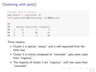
  • 14. Clustering with pam() # group into 3 clusters pam.result - pam(iris2, 3) table(pam.result$clustering, iris$Species) ## ## setosa versicolor virginica ## 1 50 0 0 ## 2 0 48 14 ## 3 0 2 36 Three clusters: I Cluster 1 is species setosa and is well separated from the other two. I Cluster 2 is mainly composed of versicolor, plus some cases from virginica. I The majority of cluster 3 are virginica, with two cases from versicolor. 13 / 30
  • 15. layout(matrix(c(1, 2), 1, 2)) # 2 graphs per page plot(pam.result) clusplot(pam(x = iris2, k = 3)) −3 −2 −1 0 1 2 3 −3 −2 −1 0 1 2 Component 1 Component 2 Silhouette plot of pam(x = iris2, k = 3) n = 150 3 clusters Cj j : nj | aveiÎCj si 1 : 50 | 0.80 2 : 62 | 0.42 3 : 38 | 0.45 0.0 0.2 0.4 0.6 0.8 1.0 Silhouette width si These two components explain 95.81 % of the point variability. Average silhouette width : 0.55 layout(matrix(1)) # change back to one graph per page 14 / 30
  • 16. Results of Clustering I In this example, the result of pam() seems better, because it identi
  • 17. es three clusters, corresponding to three species. I Note that we cheated by setting k = 3 when using pam(), which is already known to us as the number of species. 15 / 30
  • 18. Outline Introduction The k-Means Clustering The k-Medoids Clustering Hierarchical Clustering Density-based Clustering Online Resources 16 / 30
  • 19. Hierarchical Clustering of the iris Data set.seed(2835) # draw a sample of 40 records from the iris data, so that the # clustering plot will not be over crowded idx - sample(1:dim(iris)[1], 40) irisSample - iris[idx, ] # remove class label irisSample$Species - NULL # hierarchical clustering hc - hclust(dist(irisSample), method = ave) # plot clusters plot(hc, hang = -1, labels = iris$Species[idx]) # cut tree into 3 clusters rect.hclust(hc, k = 3) # get cluster IDs groups - cutree(hc, k = 3) 17 / 30
  • 20. setosa setosa setosa setosa setosa setosa setosa setosa setosa setosa setosa setosa setosa setosa versicolor versicolor versicolor virginica virginica versicolor versicolor versicolor versicolor versicolor versicolor versicolor versicolor versicolor versicolor versicolor versicolor versicolor virginica virginica virginica virginica virginica virginica virginica virginica 0 1 2 3 4 Cluster Dendrogram hclust (*, average) dist(irisSample) Height 18 / 30
  • 21. Outline Introduction The k-Means Clustering The k-Medoids Clustering Hierarchical Clustering Density-based Clustering Online Resources 19 / 30
  • 22. Density-based Clustering I Group objects into one cluster if they are connected to one another by densely populated area I The DBSCAN algorithm from package fpc provides a density-based clustering for numeric data. I Two key parameters in DBSCAN: I eps: reachability distance, which de
  • 23. nes the size of neighborhood; and I MinPts: minimum number of points. I If the number of points in the neighborhood of point is no less than MinPts, then is a dense point. All the points in its neighborhood are density-reachable from and are put into the same cluster as . I Can discover clusters with various shapes and sizes I Insensitive to noise I The k-means algorithm tends to
  • 24. nd clusters with sphere shape and with similar sizes. 20 / 30
  • 25. Density-based Clustering of the iris data library(fpc) iris2 - iris[-5] # remove class tags ds - dbscan(iris2, eps = 0.42, MinPts = 5) # compare clusters with original class labels table(ds$cluster, iris$Species) ## ## setosa versicolor virginica ## 0 2 10 17 ## 1 48 0 0 ## 2 0 37 0 ## 3 0 3 33 I 1 to 3: identi
  • 26. ed clusters I 0: noises or outliers, i.e., objects that are not assigned to any clusters 21 / 30
  • 27. plot(ds, iris2) Sepal.Length 2.0 2.5 3.0 3.5 4.0 0.5 1.0 1.5 2.0 2.5 4.5 5.5 6.5 7.5 2.0 2.5 3.0 3.5 4.0 Sepal.Width Petal.Length 1 2 3 4 5 6 7 4.5 5.5 6.5 7.5 0.5 1.0 1.5 2.0 2.5 1 2 3 4 5 6 7 Petal.Width 22 / 30
  • 28. plot(ds, iris2[c(1, 4)]) 4.5 5.0 5.5 6.0 6.5 7.0 7.5 8.0 0.5 1.0 1.5 2.0 2.5 Sepal.Length Petal.Width 23 / 30
  • 29. plotcluster(iris2, ds$cluster) 0 1 1 1 1 1 1 1 1 1 1 1 1 1 1 1 1 1 1 1 1 1 1 1 1 1 1 1 1 1 1 1 1 11 1 1 1 1 1 1 0 1 1 1 1 1 1 1 1 2 2 2 2 2 2 2 2 2 2 2 0 2 2 2 0 2 0 2 0 2 2 2 3 3 0 2 3 2 0 3 2 2 2 2 2 0 2 2 3 2 0 2 0 2 2 2 2 0 0 2 0 3 3 3 3 3 3 0 0 0 0 0 3 3 3 0 3 3 0 0 33 0 3 0 3 3 3 0 0 0 3 3 0 0 3 3 3 3 3 3 3 3 3 −8 −6 −4 −2 0 2 −2 −1 0 1 2 3 dc 1 dc 2 24 / 30
  • 30. Prediction with Clustering Model I Label new data, based on their similarity with the clusters I Draw a sample of 10 objects from iris and add small noises to them to make a new dataset for labeling I Random noises are generated with a uniform distribution using function runif(). # create a new dataset for labeling set.seed(435) idx - sample(1:nrow(iris), 10) # remove class labels new.data - iris[idx,-5] # add random noise new.data - new.data + matrix(runif(10*4, min=0, max=0.2), nrow=10, ncol=4) # label new data pred - predict(ds, iris2, new.data) 25 / 30
  • 31. Results of Prediction table(pred, iris$Species[idx]) # check cluster labels ## ## pred setosa versicolor virginica ## 0 0 0 1 ## 1 3 0 0 ## 2 0 3 0 ## 3 0 1 2 26 / 30
  • 32. Results of Prediction table(pred, iris$Species[idx]) # check cluster labels ## ## pred setosa versicolor virginica ## 0 0 0 1 ## 1 3 0 0 ## 2 0 3 0 ## 3 0 1 2 Eight(=3+3+2) out of 10 objects are assigned with correct class labels. 26 / 30
  • 33. plot(iris2[c(1, 4)], col = 1 + ds$cluster) points(new.data[c(1, 4)], pch = +, col = 1 + pred, cex = 3) + 4.5 5.0 5.5 6.0 6.5 7.0 7.5 8.0 0.5 1.0 1.5 2.0 2.5 Sepal.Length Petal.Width + + + + + + + + + 27 / 30
  • 34. Outline Introduction The k-Means Clustering The k-Medoids Clustering Hierarchical Clustering Density-based Clustering Online Resources 28 / 30
  • 35. Online Resources I Chapter 6: Clustering, in book R and Data Mining: Examples and Case Studies http://www.rdatamining.com/docs/RDataMining.pdf I R Reference Card for Data Mining http://www.rdatamining.com/docs/R-refcard-data-mining.pdf I Free online courses and documents http://www.rdatamining.com/resources/ I RDataMining Group on LinkedIn (7,000+ members) http://group.rdatamining.com I RDataMining on Twitter (1,700+ followers) @RDataMining 29 / 30
  • 36. The End Thanks! Email: yanchang(at)rdatamining.com 30 / 30