Data structure and algorithm using java
Download as PPTX, PDF6 likes6,439 views

This presentation created for people who like to go back to basics of data structure and its implementation. This presentation mostly helps B.Tech , Bsc Computer science students as well as all programmer who wants to develop software in core areas.


![Role Of Algorithm ( contd.)
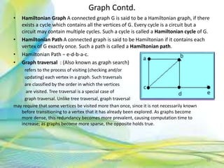
• Let us explain with an example. Consider the simplest problem of finding the G.C.D (H.C.F) of two
positive integer number m and n where n < m
• .
• E1. [Find remainder.] Divide m by n and let r be the remainder. ( 0<=r<n)
• E2. [Is it zero?] If r = 0 , the algorithm terminates; n is the answer.
• E3. [Reduce] Set m =n , n = r . go back to step E1.
• The algorithm is terminating after finite number of steps. [Finiteness]. All three steps are precisely
defined. [Definiteness]The actions carrying out are rigorous and unambiguous. It has two [ Input]
and one [Output]. Also the algorithm is effective in the sense that its operations can be done in
finite length of time.[Effectiveness]
8Neofour.com](https://image.slidesharecdn.com/datastructureandalgorithmusingjava-180530092810/85/Data-structure-and-algorithm-using-java-8-320.jpg)


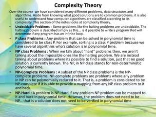
![Arrays
• Array is a fixed-size sequenced collection of variables belonging to the same data
types. The array has adjacent memory locations to store values.
• 0 (zero-based indexing): The first element of the array is indexed by subscript of 0.
• 1 (one-based indexing): The first element of the array is indexed by subscript of 1
• n (n-based indexing): The base index of an array can be freely chosen. Usually
programming languages allowing n-based indexing also allow negative index values
and other scalar data types like enumerations, or characters may be used as an
array index.
• Array Declaration /;data type Arrayname[sizeofArray]; Arrayname[row][column];
• Operations: Traversing , Inserting , Deleting , Searching , Updating
• Some language allows resizing array.
• Advantages:
– Convenient , implement linked list, stack , queue , tree , graph etc, space savings ,
• Disadvantage
o Static , Partially full , insertion , deletion in middle is costly , Bound checking require
17Neofour.com](https://image.slidesharecdn.com/datastructureandalgorithmusingjava-180530092810/85/Data-structure-and-algorithm-using-java-17-320.jpg)


![Multiple Queues
• Method 1 (Divide the array in slots of size n/k)
A simple way to implement k queues is to divide the array in k slots of size n/k each,
and fix the slots for different queues, i.e., use arr[0] to arr[n/k-1] for first queue, and
arr[n/k] to arr[2n/k-1] for queue2 where arr[] is the array to be used to implement two
queues and size of array be n.
• The problem with this method is inefficient use of array space. An enqueue operation
may result in overflow even if there is space available in arr[]. For example, consider k
as 2 and array size n as 6. Let us enqueue 3 elements to first and do not enqueue
anything to second queue. When we enqueue 4th element to first queue, there will be
overflow even if we have space for 3 more elements in array.
• Method 2 (A space efficient implementation)
The idea is similar to the stack post, here we need to use three extra arrays. In stack
post, we needed to extra arrays, one more array is required because in queues,
enqueue() and dequeue() operations are done at different ends.
• Following are the three extra arrays are used:
1) front[]: This is of size k and stores indexes of front elements in all queues.
2) rear[]: This is of size k and stores indexes of rear elements in all queues.
2) next[]: This is of size n and stores indexes of next item for all items in array arr[].
• Here arr[] is actual array that stores k stacks.
• Together with k queues, a stack of free slots in arr[] is also maintained. The top of this
stack is stored in a variable ‘free’.
• All entries in front[] are initialized as -1 to indicate that all queues are empty. All entries
next[i] are initialized as i+1 because all slots are free initially and pointing to next slot.
Top of free stack, ‘free’ is initialized as 0.
23Neofour.com](https://image.slidesharecdn.com/datastructureandalgorithmusingjava-180530092810/85/Data-structure-and-algorithm-using-java-23-320.jpg)


![Bubble Sort
32Neofour.com
for(int k = 0; k< n-1; k++) {
for(int i = 0; i < n-k-1; i++) {
if(A[ i ] > A[ i+1] ) { swap( A[i] ,
A[I + 1]}
}
}
Complexity:
Worst and Average Case Time Complexity: O(n*n). Worst case occurs when array is
reverse sorted.
Best Case Time Complexity: O(n). Best case occurs when array is already sorted.
Auxiliary Space: O(1)
Boundary Cases: Bubble sort takes minimum time (Order of n) when elements are
already sorted.
Sorting In Place: Yes
Stable: Yes](https://image.slidesharecdn.com/datastructureandalgorithmusingjava-180530092810/85/Data-structure-and-algorithm-using-java-32-320.jpg)


![Searching
• A search algorithm is any algorithm which solves the Search problem,
namely, to retrieve information stored within some data structure.
Examples of such structures include but are not limited to a Linked List,
an Array data structure, or a Search tree. Searching also encompasses
algorithms that query the data structure, such as the SQL SELECT
command.
• Linear Search
– A simple approach is to do linear search, i.e. Start from the leftmost element of arr[] and
one by one compare x with each element of arr[]
– If x matches with an element, return the index.
– If x doesn’t match with any of elements, return -1.
• Binary Search
– Compare x with the middle element.
– If x matches with middle element, we return the mid index.
– Else If x is greater than the mid element, then x can only lie in right half subarray after
the mid element. So we recur for right half.
– Else (x is smaller) recur for the left half.
41Neofour.com](https://image.slidesharecdn.com/datastructureandalgorithmusingjava-180530092810/85/Data-structure-and-algorithm-using-java-41-320.jpg)

![Search contd.
• Interpolation Search : The Interpolation Search is an improvement over Binary
Search for instances, where the values in a sorted array are uniformly distributed.
Binary Search always goes to middle element to check. On the other hand
interpolation search may go to different locations according the value of key being
searched. For example if the value of key is closer to the last element,
interpolation search is likely to start search toward the end side.
– pos = lo + [ (x-arr[lo])*(hi-lo) / (arr[hi]-arr[Lo]) ] arr[]
– ==> Array where elements need to be searched
– x ==> Element to be searched
– lo ==> Starting index in arr[]
– hi ==> Ending index in arr[]
• Step1: In a loop, calculate the value of “pos” using the probe position formula.
Step2: If it is a match, return the index of the item, and exit.
Step3: If the item is less than arr[pos], calculate the probe position of the left
sub-array. Otherwise calculate the same in the right sub-array.
Step4: Repeat until a match is found or the sub-array reduces to zero.
• Time Complexity : If elements are uniformly distributed, then O (log log n)). In
worst case it can take up to O(n).
Auxiliary Space : O(1)
43Neofour.com](https://image.slidesharecdn.com/datastructureandalgorithmusingjava-180530092810/85/Data-structure-and-algorithm-using-java-43-320.jpg)


![Search contd.
• Fibonacci Search
• Given a sorted array arr[] of size n and an element x to be searched in it.
Return index of x if it is present in array else return -1.
Examples: Input: arr[] = {2, 3, 4, 10, 40}, x = 10 , Output: 3 , Element x is
present at index 3.
• Input: arr[] = {2, 3, 4, 10, 40}, x = 11 , Output: -1 Element x is not present.
• Fibonacci Search is a comparison-based technique that uses Fibonacci
numbers to search an element in a sorted array.
• Similarities with Binary Search:
– Works for sorted arrays
– A Divide and Conquer Algorithm.
– Has Log n time complexity.
• Differences with Binary Search:
– Fibonacci Search divides given array in unequal parts
– Binary Search uses division operator to divide range. Fibonacci Search doesn’t use /, but
uses + and -
46Neofour.com](https://image.slidesharecdn.com/datastructureandalgorithmusingjava-180530092810/85/Data-structure-and-algorithm-using-java-46-320.jpg)
![Fibonacci Search contd.
• Algorithm:
• Let arr[0..n-1] be th input array and element to be searched be x.
• Find the smallest Fibonacci Number greater than or equal n. Let this number
be fibM [math Fibonacci Number]. Let the two Fibonacci numbers preceding it
be fibMm1 [(m-1)’th Fibonacci Number] and fibMm2 [(m-2)’th Fibonacci
Number].
• While the array has elements to be inspected:
• Compare x with the last element of the range covered by fibMm2
• If x matches, return index
• Else If x is less than the element, move the three Fibonacci variables two
Fibonacci down, indicating elimination of approximately rear two-third of the
remaining array.
• Else x is greater than the element, move the three Fibonacci variables one
Fibonacci down. Reset offset to index. Together these indicate elimination of
approximately front one-third of the remaining array.
• Since there might be a single element remaining for comparison, check if
fibMm1 is 1. If Yes, compare x with that remaining element. If match, return
index.
47Neofour.com](https://image.slidesharecdn.com/datastructureandalgorithmusingjava-180530092810/85/Data-structure-and-algorithm-using-java-47-320.jpg)


![B Trees (or general m-way search trees)
• Search tree called B-Tree in which a node can store more than one value (key) and
it can have more than two children. B-Tree was developed in the year of 1972
by Bayer and McCreight with the name Height Balanced m-way Search Tree. Later
it was named as B-Tree.
B-Tree is a self-balanced search tree with multiple keys in every node and more
than two children for every node.
• B-Tree of Order m has the following properties...
• Property #1 - All the leaf nodes must be at same level.
• Property #2 - All nodes except root must have at least [m/2]-1 keys and maximum
of m-1 keys.
• Property #3 - All non leaf nodes except root (i.e. all internal nodes) must have at
least m/2 children.
• Property #4 - If the root node is a non leaf node, then it must have at least
2 children.
• Property #5 - A non leaf node with n-1 keys must have n number of children.
• Property #6 - All the key values within a node must be in Ascending Order.
• For example, B-Tree of Order 4 contains maximum 3 key values in a node and
maximum 4 children for a node.
62Neofour.com](https://image.slidesharecdn.com/datastructureandalgorithmusingjava-180530092810/85/Data-structure-and-algorithm-using-java-62-320.jpg)


![Java Map Interface program
import java.util.*;
public class MapInterfaceExample {
public static void main(String args[] ) {
HashMap <Integer,String> map = new HashMap <Integer,String> ();
map.put(100,"Amit");
map.put(101,"Vijay");
map.put(102,"Rahul");
map.put(101, "narayan");
for(HashMap.Entry m:map.entrySet()){
System.out.println(m.getKey()+" "+m.getValue());
}
}
}
75Neofour.com](https://image.slidesharecdn.com/datastructureandalgorithmusingjava-180530092810/85/Data-structure-and-algorithm-using-java-75-320.jpg)


![Graph Representation
• Adjacency Matrix is a 2D array of size V x V where V is the number of vertices in a graph.
Let the 2D array be adj[][], a slot adj[i][j] = 1 indicates that there is an edge from vertex i to
vertex j. Adjacency matrix for undirected graph is always symmetric. Adjacency Matrix is also
used to represent weighted graphs. If adj[i][j] = w, then there is an edge from vertex i to
vertex j with weight w.
• The adjacency matrix for the graph is:
– Pros: Representation is easier to implement and follow. Removing an edge takes O(1) time. Queries
like whether there is an edge from vertex ‘u’ to vertex ‘v’ are efficient and can be done O(1).
– Cons: Consumes more space O(V^2). Even if the graph is sparse(contains less number of edges), it
consumes the same space. Adding a vertex is O(V^2) time.
• Adjacency List : An array of linked lists is used. Size of the array
is equal to number of vertices. Let the array be array[]. An entry array[i]
represents the linked list of vertices adjacent to the ith vertex. This
representation can also be used to represent a weighted graph. The
weights of edges can be stored in nodes of linked lists. Following is
adjacency list representation of the above graph.
80Neofour.com](https://image.slidesharecdn.com/datastructureandalgorithmusingjava-180530092810/85/Data-structure-and-algorithm-using-java-80-320.jpg)


Ad
More Related Content
What's hot (20)
Similar to Data structure and algorithm using java (20)


Ad
Recently uploaded (20)


Ad
Data structure and algorithm using java
- 1. Data Structure and Algorithm Using Java Narayan Sau 1Neofour.com
- 2. Syllabus • Role of Algorithm • Role of Data Structure • Algorithm Design • Types of Data Structure • Algorithm Analysis • Random Access Machine model • Abstract Data Type • Primitive data types • Array & Structure • Stack operations • Evaluation expression • Infix , postfix , prefix • Queue operations • Stack , Queue implementation using Array , Link list • Circular Queue Neofour.com 2
- 3. Syllabus • Priority Queue • Application of Queue, Stack • Singly , Doubly , Circular link list and operations • Link List implementation using ADT and Interface in Java. • Advantage and Disadvantages of link list • Polynomial Implementation • Sorting & Searching • Sorting Algorithm ( Bubble, Selection , Merge , Quick , Heap, radix sorts ) • Searching algorithm ( Linear , binary , Jump , Interpolation , Exponential , Fibonacci) • Trees ( example , Terminology) • Types of Tree ( binary , BST , AVL , B tree , B+ tree, 2-3 tree, Red Back tree) Neofour.com 3
- 4. Syllabus • Link list , Heap implementation of tree. • Huffman tree presentation • Tree traversal ( pre, in , post order) • MAP • Hash 4Neofour.com
- 5. Syllabus • Graph introduction , terminology • Representation – Adjacency matrix , Adjacency list • Traversing graph • Connectivity • DFS , BFS • Spanning tree • Kirchoff’s , Prim , Kruskal , Greedy algorithm • Complexity Theory 5Neofour.com
- 6. Role Of Algorithm • An algorithm is a procedure to solve a problem in mathematical terms. • It is the mathematical counterpart to programs. • The Essential concept to build efficient systems in space and time complexity and develop ones problem solving skills. • Provides the right set of techniques for data handling 6Neofour.com
- 7. Role Of Algorithm ( contd.) • Finiteness. An algorithm must always terminate after a finite number of steps. • Definiteness. Each step of an algorithm must be precisely defined down to the last detail. The action to be carried out must be rigorously and unambiguously specified for each case. • Input. An algorithm has zero or more inputs. • Output. An algorithm has one or more outputs. • Effectiveness. An algorithm is also generally expected to be effective, in the sense that its operations must all be sufficiently basic that they can in principle be done exactly and in a finite length of time by someone using pencil and paper. 7Neofour.com
- 8. Role Of Algorithm ( contd.) • Let us explain with an example. Consider the simplest problem of finding the G.C.D (H.C.F) of two positive integer number m and n where n < m • . • E1. [Find remainder.] Divide m by n and let r be the remainder. ( 0<=r<n) • E2. [Is it zero?] If r = 0 , the algorithm terminates; n is the answer. • E3. [Reduce] Set m =n , n = r . go back to step E1. • The algorithm is terminating after finite number of steps. [Finiteness]. All three steps are precisely defined. [Definiteness]The actions carrying out are rigorous and unambiguous. It has two [ Input] and one [Output]. Also the algorithm is effective in the sense that its operations can be done in finite length of time.[Effectiveness] 8Neofour.com
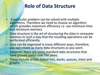
- 9. Role of Data Structure • A particular problem can be solved with multiple algorithms. Therefore we need to choose an algorithm which provides maximum efficiency i.e. use minimum time and minimum memory • Data structure is the art of structuring the data in computer memory in such a way that the resulting operations can be performed efficiently. • Data can be organized in many different ways; therefore, you can create as many data structures as you want. • However, there are some standard data structures that have proved useful over the years. • These include arrays, linked lists, stacks, queues, trees and graphs. 9Neofour.com
- 10. Algorithm Design • To solve our real world problem we need real world solution. • Brute Force • Greedy Algorithms "take what you can get now“ strategy • Divide-and-Conquer , Decrease-and-Conquer • Dynamic Programming • Transform-and-Conquer • Back tracking and branch -and-bound 10Neofour.com
- 11. Types of Data Structure • Primitive types Boolean , Character Floating-point, Real, Double , Integer, String, Reference , Enumerated type • Composite types or Non-primitive type Array , record • Abstract data types Container ,List, Associative array , Set , Stack, Queue, Double-ended queue , Tree , Graph 11Neofour.com
- 12. Algorithm Analysis • Time and Space complexity – Time Factor − Time is measured by counting the number of key operations such as comparisons in the sorting algorithm. – Space Factor − Space is measured by counting the maximum memory space required by the algorithm • A Priori Analysis – This is a theoretical analysis of an algorithm. Efficiency of an algorithm is measured by assuming that all other factors, for example, processor speed, are constant and have no effect on the implementation. • A Posterior Analysis – This is an empirical analysis of an algorithm. The selected algorithm is implemented using programming language. This is then executed on target computer machine. In this analysis, actual statistics like running time and space required, are collected. 12Neofour.com
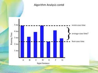
- 14. Asymptotic notations • Big Oh Notation, Ο – The notation Ο(n) is the formal way to express the upper bound of an algorithm's running time. It measures the worst case time. Let f(n) and g(n) be functions mapping non negative integers to real numbers. We say that f(n) is O(g(n)) if there is a real constant c >0 and an integer constant n0 >= 1 such that f(n) <=cg(n) , for n > n0. Then f(n) is big-Oh of g(n). • Omega Notation, Ω – The notation Ω(n) is the formal way to express the lower bound of an algorithm's running time. It measures the best case time complexity or the best amount of time an algorithm can possibly take to complete. If f(n) >= c.g(n) for c = constant and n > n0. Then we say f(n) is Ω(g(n)) • Theta Notation, θ – Theta, commonly written as Θ, is an Asymptotic Notation to denote the asymptotically tight bound on the growth rate of runtime of an algorithm. f(n) is Θ(g(n)), if for some real constants c1, c2 and n0 (c1 > 0, c2 > 0, n0 > 0), c1 g(n) is < f(n) is < c2 g(n) for every input size n (n > n0). f(n) is Θ(g(n)) implies f(n) is O(g(n)) as well as f(n) is Ω(g(n)). The notation θ(n) is the formal way to express both the lower bound and the upper bound of an algorithm's running time. It is represented as follows − 14Neofour.com
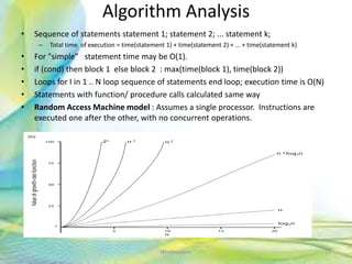
- 15. Algorithm Analysis • Sequence of statements statement 1; statement 2; ... statement k; – Total time of execution = time(statement 1) + time(statement 2) + ... + time(statement k) • For "simple" statement time may be O(1). • if (cond) then block 1 else block 2 : max(time(block 1), time(block 2)) • Loops for I in 1 .. N loop sequence of statements end loop; execution time is O(N) • Statements with function/ procedure calls calculated same way • Random Access Machine model : Assumes a single processor. Instructions are executed one after the other, with no concurrent operations. 15Neofour.com
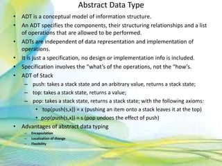
- 16. Abstract Data Type • ADT is a conceptual model of information structure. • An ADT specifies the components, their structuring relationships and a list of operations that are allowed to be performed. • ADTs are independent of data representation and implementation of operations. • It is just a specification, no design or implementation info is included. • Specification involves the “what’s of the operations, not the “how’s. • ADT of Stack – push: takes a stack state and an arbitrary value, returns a stack state; – top: takes a stack state, returns a value; – pop: takes a stack state, returns a stack state; with the following axioms: • top(push(s,x)) = x (pushing an item onto a stack leaves it at the top) • pop(push(s,x)) = s (pop undoes the effect of push) • Advantages of abstract data typing – Encapsulation – Localization of change – Flexibility 16Neofour.com
- 17. Arrays • Array is a fixed-size sequenced collection of variables belonging to the same data types. The array has adjacent memory locations to store values. • 0 (zero-based indexing): The first element of the array is indexed by subscript of 0. • 1 (one-based indexing): The first element of the array is indexed by subscript of 1 • n (n-based indexing): The base index of an array can be freely chosen. Usually programming languages allowing n-based indexing also allow negative index values and other scalar data types like enumerations, or characters may be used as an array index. • Array Declaration /;data type Arrayname[sizeofArray]; Arrayname[row][column]; • Operations: Traversing , Inserting , Deleting , Searching , Updating • Some language allows resizing array. • Advantages: – Convenient , implement linked list, stack , queue , tree , graph etc, space savings , • Disadvantage o Static , Partially full , insertion , deletion in middle is costly , Bound checking require 17Neofour.com
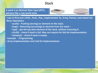
- 18. Stack A stack is an Abstract Data Type (ADT), behaves like a real-world stack 18Neofour.com • Last-in-first-out ( LIFO) , Push , Pop , implemented by Array, Pointer, and Linked List. •Basic Operations • push() − Pushing (storing) an element on the stack. • pop() − Removing (accessing) an element from the stack.− • top() − get the top data element of the stack, without removing it. • isFull() − check if stack is full. May not require for link list implementation. • isEmpty() − check if stack is empty. • Example : Programming. • Array Implementation and Link list implementation.
- 19. Queue 19Neofour.com • A linear structure which follows a particular order in which the operations are performed. The order is First In First Out (FIFO). • Queue is used when things don’t have to be processed immediately, but have to be processed in First In First Out order. • When a resource is shared among multiple consumers. Examples include CPU scheduling, Disk Scheduling. • When data is transferred asynchronously (data not necessarily received at same rate as sent) between two processes. Examples include IO Buffers, pipes, file IO, etc. • Basic operation •Enqueue: Adds an item to the queue. If the queue is full, then it is said to be an Overflow condition. •Dequeue: Removes an item from the queue. The items are popped in the same order in which they are pushed. If the queue is empty, then it is said to be an Underflow condition. •Rear: Get the last item from queue. •Front () , peek() − Gets the element at the front of the queue without removing it. •isfull() − Checks if the queue is full. •isempty() − Checks if the queue is empty.
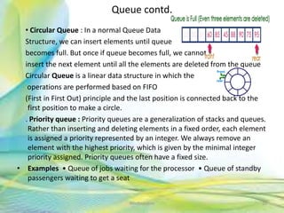
- 20. Queue contd. • Circular Queue : In a normal Queue Data Structure, we can insert elements until queue becomes full. But once if queue becomes full, we cannot insert the next element until all the elements are deleted from the queue Circular Queue is a linear data structure in which the operations are performed based on FIFO (First in First Out) principle and the last position is connected back to the first position to make a circle. . Priority queue : Priority queues are a generalization of stacks and queues. Rather than inserting and deleting elements in a fixed order, each element is assigned a priority represented by an integer. We always remove an element with the highest priority, which is given by the minimal integer priority assigned. Priority queues often have a fixed size. • Examples • Queue of jobs waiting for the processor • Queue of standby passengers waiting to get a seat 20Neofour.com
- 21. Priority Queue • Basic Operations: – size() return the number of entries in PQ – isEmpty() test whether PQ is empty – min() return (but not remove) the entry with the smallest key – insert(k, x) insert value x with key k – removeMin() remove from PQ and return the entry with the smallest key (k,v) key=integer, value=letter – Example • PQ={} • insert(5,A) PQ={(5,A)} • insert(9,C) PQ={(5,A), (9,C)} • insert(3,B) PQ={(5,A), (9,C), (3,B)} • insert(7,D) PQ={(5,A), (7,D), (9,C), (3,B)} • min() return (3,B) • removeMin() PQ = {(5,A), (7,D), (9,C)} • size() return 3 • removeMin() return (5,A) PQ={(7,D), (9,C)} • removeMin() return (7,D) PQ={(9,C)} • removeMin() return (9,C) PQ={} • An important application of a priority queue is sorting PriorityQueueSort (collection S of n elements) • put the elements in S in an initially empty priority queue by means of a series of n insert() operations on the pqueue, one for each element • extract the elements from the pqueue by means of a series of n removeMin() operations. 21Neofour.com
- 22. Adaptable Priority Queues • A standby passenger with a pessimistic attitude may become tired of waiting and decide to leave ahead of the boarding time, requesting to be removed from the waiting list. Thus, we would like to remove from the priority queue the entry associated with this passenger. Operation removeMin is not suitable for this purpose since the passenger leaving is unlikely to have first priority. Instead, we would like to have a new operation remove (e) that removes an arbitrary entry e. • Another standby passenger finds her gold frequent-flyer card and shows it to the agent. Thus, her priority has to be modified accordingly. To achieve this change of priority, we would like to have a new operation replaceKey(e,k) that replaces with k the key of entry e in the priority queue. • Finally, a third standby passenger notices her name is misspelled on the ticket and asks it to be corrected. To perform the change, we need to update the passenger's record. Hence, we would like to have a new operation replace Value(e,x) that replaces with x the value of entry e in the priority queue 22Neofour.com
- 23. Multiple Queues • Method 1 (Divide the array in slots of size n/k) A simple way to implement k queues is to divide the array in k slots of size n/k each, and fix the slots for different queues, i.e., use arr[0] to arr[n/k-1] for first queue, and arr[n/k] to arr[2n/k-1] for queue2 where arr[] is the array to be used to implement two queues and size of array be n. • The problem with this method is inefficient use of array space. An enqueue operation may result in overflow even if there is space available in arr[]. For example, consider k as 2 and array size n as 6. Let us enqueue 3 elements to first and do not enqueue anything to second queue. When we enqueue 4th element to first queue, there will be overflow even if we have space for 3 more elements in array. • Method 2 (A space efficient implementation) The idea is similar to the stack post, here we need to use three extra arrays. In stack post, we needed to extra arrays, one more array is required because in queues, enqueue() and dequeue() operations are done at different ends. • Following are the three extra arrays are used: 1) front[]: This is of size k and stores indexes of front elements in all queues. 2) rear[]: This is of size k and stores indexes of rear elements in all queues. 2) next[]: This is of size n and stores indexes of next item for all items in array arr[]. • Here arr[] is actual array that stores k stacks. • Together with k queues, a stack of free slots in arr[] is also maintained. The top of this stack is stored in a variable ‘free’. • All entries in front[] are initialized as -1 to indicate that all queues are empty. All entries next[i] are initialized as i+1 because all slots are free initially and pointing to next slot. Top of free stack, ‘free’ is initialized as 0. 23Neofour.com
- 24. Applications of Queue & Stack Data Structure • Imagine you have a web-site which serves files to thousands of users. You cannot service all requests, you can only handle say 100 at once. A fair policy would be first-come-first serve: serve 100 at a time in order of arrival. – Data Buffers – Asynchronous data transfer (file IO, pipes, sockets). – Dispensing requests on a shared resource (printer, processor). – Traffic analysis. – Determine the number of cashiers to have at a supermarket. • Stacks are used for the undo buttons in various software. The recent most changes are pushed into the stack. Even the back button on the browser works with the help of the stack where all the recently visited web pages are pushed into the stack. – Parsing in a compiler. – Java virtual machine. – Undo in a word processor. – Back button in a Web browser. – Implementing function calls in a compiler. 24Neofour.com
- 25. Comparison Chart BASIS FOR COMPARISON STACK QUEUE Working principle LIFO (Last in First out) FIFO (First in First out) Structure Same end is used to insert and delete elements. One end is used for insertion, i.e., rear end and another end is used for deletion of elements, i.e., front end. Number of pointers used One Two (In simple queue case) Operations performed Push and Pop Enqueue and dequeue Examination of empty condition Top == -1 Front == -1 || Front == Rear + 1 Examination of full condition Top == Max - 1 Rear == Max - 1 Variants It does not have variants. It has variants like circular queue, priority queue, doubly ended queue. Implementation Simpler Comparatively complex 25Neofour.com
- 26. Link List • Linked list is a sequence of data linked with each other. Linked list elements are not stored at contiguous location; the elements are linked using pointers. 26Neofour.com Pros : Dynamic size , Ease of insertion/deletion Cons : 1) Random access is not allowed. We have to access elements sequentially starting from the first node. So we cannot do binary search with linked lists. 2) Extra memory space for a pointer is required with each element of the list. In a singly linked list each node in the list stores the contents of the node and a pointer or reference to the next node in the list. It does not store any pointer or reference to the previous node. In a single linked list, the insertion operation can be performed in three ways. They are as follows... •Inserting at Beginning of the list •Inserting at End of the list •Inserting at Specific location in the list
- 27. Insertion Operations • Inserting At Beginning of the list • We can use the following steps to insert a new node at beginning of the single linked list... • Step 1: Create a newNode with given value. • Step 2: Check whether list is Empty (head == NULL) • Step 3: If it is Empty then, set newNode→next = NULL and head = newNode. • Step 4: If it is Not Empty then, set newNode→next = head and head = newNode. • Inserting At End of the list • We can use the following steps to insert a new node at end of the single linked list... • Step 1: Create a newNode with given value and newNode → next as NULL. • Step 2: Check whether list is Empty (head == NULL). • Step 3: If it is Empty then, set head = newNode. • Step 4: If it is Not Empty then, define a node pointer temp and initialize with head. • Step 5: Keep moving the temp to its next node until it reaches to the last node in the list (until temp → next is equal to NULL). • Step 6: Set temp → next = newNode. • Inserting At Specific location in the list (After a Node) • We can use the following steps to insert a new node after a node in the single linked list... • Step 1: Create a newNode with given value. • Step 2: Check whether list is Empty (head == NULL) • Step 3: If it is Empty then, set newNode → next = NULL and head = newNode. • Step 4: If it is Not Empty then, define a node pointer temp and initialize with head. • Step 5: Keep moving the temp to its next node until it reaches to the node after which we want to insert the newNode (until temp1 → data is equal to location, here location is the node value after which we want to insert the newNode). • Step 6: Every time check whether temp is reached to last node or not. If it is reached to last node then display 'Given node is not found in the list!!! Insertion not possible!!!' and terminate the function. Otherwise move the temp to next node. • Step 7: Finally, Set 'newNode → next = temp → next' and 'temp → next = newNode' 27Neofour.com
- 28. Deletion & Display • Deletion – In a single linked list, the deletion operation can be performed in three ways. They are as follows... – Deleting from Beginning of the list – Deleting from End of the list – Deleting a Specific Node • Displaying a Single Linked List We can use the following steps to display the elements of a single linked list... – Step 1: Check whether list is Empty (head == NULL) – Step 2: If it is Empty then, display 'List is Empty!!!' and terminate the function. – Step 3: If it is Not Empty then, define a Node pointer 'temp' and initialize with head. – Step 4: Keep displaying temp → data with an arrow (--->) until temp reaches to the last node – Step 5: Finally display temp → data with arrow pointing to NULL (temp → data ---> NULL). 28Neofour.com
- 29. Circular /Doubly link List • In single linked list, every node points to its next node in the sequence and the last node points NULL. But in circular linked list, every node points to its next node in the sequence but the last node points to the first node in the list. • Circular linked list is a sequence of elements in which every element has link to its next element in the sequence and the last element has a link to the first element in the sequence. 29Neofour.com In a single linked list, we can traverse from one node to other node only in one direction and we cannot traverse back. Doubly linked list is a sequence of elements in which every element has links to its previous element and next element in the sequence. Doubly Circular Link List
- 30. Advantage and Disadvantages of link List • Advantage : Dynamic Data Structure, can grow and shrink at runtime by allocating and deallocating memory. • Insertion and deletion of nodes are really easier, just have to update the address present in next pointer of a node. • size of linked list can increase or decrease at run time so there is no memory wastage. • Data structures such as stack and queues can be easily implemented using linked list. • Disadvantages : More memory is required to store elements in linked list as compared to array. Because in linked list each node contains a pointer and it requires extra memory for itself. • Traversal Elements or nodes traversal is difficult in linked list. We cannot randomly access any element as we do in array by index. • Reverse traversing is really difficult. In case of doubly linked list its easier but extra memory is required for back pointer hence wastage of memory. • Operations : Creation, Insertion, Deletion, Traversing, Searching, Concatenation 30Neofour.com
- 31. Sorting • Sorting is a process of organizing a collection of data into either ascending or descending order. Given a set of records r1, r2, ..., rn with key values k1, k2, ..., kn, the Sorting Problem is to arrange the records into any order s such that records rs1 , rs2 , ..., rsn have keys obeying the property ks1 <= ks2 <= ::: <= ksn. In other words, the sorting problem is to arrange a set of records so that the values of their key fields are in non-decreasing order. • A sorting algorithm is said to be stable if it does not change the relative ordering of records with identical key values. • a. internal b. external sorting. • An internal sorting requires that the collection of data fit entirely in the computers main memory • When collection of data does not fit entirely in main memory but resides in secondary in secondary memory ( e;g; disk) and algorithm needs to develop differently for doing external sorts. 31www.Neofour.com
- 32. Bubble Sort 32Neofour.com for(int k = 0; k< n-1; k++) { for(int i = 0; i < n-k-1; i++) { if(A[ i ] > A[ i+1] ) { swap( A[i] , A[I + 1]} } } Complexity: Worst and Average Case Time Complexity: O(n*n). Worst case occurs when array is reverse sorted. Best Case Time Complexity: O(n). Best case occurs when array is already sorted. Auxiliary Space: O(1) Boundary Cases: Bubble sort takes minimum time (Order of n) when elements are already sorted. Sorting In Place: Yes Stable: Yes
- 33. Selection sort • Imagine some data that you can examine all at once. To sort it, you could select the largest item and put it in its place, select the next largest and put it in its place and so on. The same what a card player does. • The algorithm maintains two sub arrays in a given array. • 1) The sub array which is already sorted. 2) Remaining sub array which is unsorted. • In every iterations of selection sort, the minimum element (considering ascending order) from the unsorted sub array is picked and moved to the sorted sub array 33Neofour.com Algorithm Step 1 − Set MIN to location 0 Step 2 − Search the minimum element in the list Step 3 − Swap with value at location MIN Step 4 − Increment MIN to point to next element Step 5 − Repeat until list is sorted Time Complexity: O(n2) as there are two nested loops. Auxiliary Space: O(1) The good thing about selection sort is it never makes more than O(n) swaps and can be useful when memory write is a costly operation.
- 34. Insertion sort 34Neofour.com Algorithm Step 1 − If it is the first element, it is already sorted. Return 1; Step 2 − Pick next element Step 3 − Compare with all elements in the sorted sub-list Step 4 − Shift all the elements in the sorted sub-list that is greater than the value to be sorted Step 5 − Insert the value Step 6 − Repeat until list is sorted Time Complexity: O(n*n) Auxiliary Space: O(1) Boundary Cases: Insertion sort takes maximum time to sort if elements are sorted in reverse order. And it takes minimum time (Order of n) when elements are already sorted. Algorithmic Paradigm: Incremental Approach Sorting In Place: Yes Stable: Yes Online: Yes
- 35. Divide-and-conquer • Divide: If the input size is smaller than a certain threshold (say, one or two elements), solve the problem directly using a straightforward method and return the solution so obtained. Otherwise, divide the input data into two or more disjoint subsets. • Conquer: Recursively solve the sub problems associated with the subsets. • Combine: Take the solutions to the sub problems and merge them into a solution to the original problem. 35Neofour.com
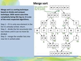
- 36. Merge sort 36Neofour.com Merge sort is a sorting technique based on divide and conquer technique. With worst-case time complexity being Ο(n log n), it is one of the most respected algorithms. Step 1 − if it is only one element in the list it is already sorted, return. Step 2 − divide the list recursively into two halves until it can no more be divided. Step 3 − merge the smaller lists into new list in sorted order.
- 37. Quick sort 37Neofour.com Quick sort is a highly efficient sorting algorithm and is based on partitioning of array of data into smaller arrays. A large array is partitioned into two arrays one of which holds values smaller than the specified value, say pivot, based on which the partition is made and another array holds values greater than the pivot value. There are many different versions of quick Sort that pick pivot in different ways. Always pick first element as pivot. Always pick last element as pivot (implemented below) Pick a random element as pivot. Pick median as pivot. Worst Case: O(n2) , Best Case , Average Case : O( n log n)
- 38. Heap sort • A complete binary tree is a binary tree in which every level, except possibly the last, is completely filled, and all nodes are as far left as possible. • A Binary Heap is a Complete Binary Tree where items are stored in a special order such that value in a parent node is greater(or smaller) than the values in its two children nodes. The former is called as max heap and the latter is called min heap. The heap can be represented by binary tree or array. • Since a Binary Heap is a Complete Binary Tree, it can be easily represented as array and array based representation is space efficient. If the parent node is stored at index I, the left child can be calculated by 2 * I + 1 and right child by 2 * I + 2 (assuming the indexing starts at 0). • Heap sort is a comparison based sorting technique based on Binary Heap data structure. It is similar to selection sort where we first find the maximum element and place the maximum element at the end. We repeat the same process for remaining element. • max_heapify has complexity O(logN), build_maxheap has complexity O(N) and we run max_heapify N−1times in heap_sort function, therefore complexity of heap_sort function is O(NlogN). 38Neofour.com
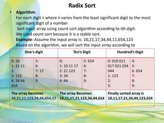
- 40. Radix Sort • Algorithm: For each digit ii where ii varies from the least significant digit to the most significant digit of a number Sort input array using count sort algorithm according to ith digit. We used count sort because it is a stable sort. Example: Assume the input array is: 10,21,17,34,44,11,654,123 Based on the algorithm, we will sort the input array according to 40Neofour.com One's digit Ten’s Digit Hundred’s Digit 0: 10 1: 21 11 2: 3: 123 4: 34 44 654 5: 6: 7: 17 8: 9: 0: 1: 10 11 17 2: 21 123 3: 34 4: 44 5: 654 6: 7: 8: 9: 0: 010 011 017 021 034 044 1: 123 2: 3: 4: 5: 6: 654 7: 8: 9: The array becomes 10,21,11,123,24,44,654,17 The array Becomes 10,11,17,21,123,34,44,654 Finally sorted array is 10,11,17,21,34,44,123,654
- 41. Searching • A search algorithm is any algorithm which solves the Search problem, namely, to retrieve information stored within some data structure. Examples of such structures include but are not limited to a Linked List, an Array data structure, or a Search tree. Searching also encompasses algorithms that query the data structure, such as the SQL SELECT command. • Linear Search – A simple approach is to do linear search, i.e. Start from the leftmost element of arr[] and one by one compare x with each element of arr[] – If x matches with an element, return the index. – If x doesn’t match with any of elements, return -1. • Binary Search – Compare x with the middle element. – If x matches with middle element, we return the mid index. – Else If x is greater than the mid element, then x can only lie in right half subarray after the mid element. So we recur for right half. – Else (x is smaller) recur for the left half. 41Neofour.com
- 42. Jump Search • Jump Search • The basic idea is to check fewer elements (than linear search) by jumping ahead by fixed steps or skipping some elements in place of searching all elements. • Let’s consider the following array: (0, 1, 1, 2, 3, 5, 8, 13, 21, 34, 55, 89, 144, 233, 377, 610). Length of the array is 16. Jump search will find the value of 55 with the following steps assuming that the block size to be jumped is 4. STEP 1: Jump from index 0 to index 4; STEP 2: Jump from index 4 to index 8; STEP 3: Jump from index 8 to index 16; STEP 4: Since the element at index 16 is greater than 55 we will jump back a step to come to index 9. STEP 5: Perform linear search from index 9 to get the element 55. • What is the optimal block size to be skipped? In the worst case, we have to do n/m jumps and if the last checked value is greater than the element to be searched for, we perform m-1 comparisons more for linear search. Therefore the total number of comparisons in the worst case will be ((n/m) + m-1). The value of the function ((n/m) + m-1) will be minimum when m = √n. Therefore, the best step size is m = √n. 42Neofour.com
- 43. Search contd. • Interpolation Search : The Interpolation Search is an improvement over Binary Search for instances, where the values in a sorted array are uniformly distributed. Binary Search always goes to middle element to check. On the other hand interpolation search may go to different locations according the value of key being searched. For example if the value of key is closer to the last element, interpolation search is likely to start search toward the end side. – pos = lo + [ (x-arr[lo])*(hi-lo) / (arr[hi]-arr[Lo]) ] arr[] – ==> Array where elements need to be searched – x ==> Element to be searched – lo ==> Starting index in arr[] – hi ==> Ending index in arr[] • Step1: In a loop, calculate the value of “pos” using the probe position formula. Step2: If it is a match, return the index of the item, and exit. Step3: If the item is less than arr[pos], calculate the probe position of the left sub-array. Otherwise calculate the same in the right sub-array. Step4: Repeat until a match is found or the sub-array reduces to zero. • Time Complexity : If elements are uniformly distributed, then O (log log n)). In worst case it can take up to O(n). Auxiliary Space : O(1) 43Neofour.com
- 44. Search contd. • Exponential Search • Exponential search involves two steps: – Find range where element is present – Do Binary Search in above found range. • Time Complexity : O(Log n) Auxiliary Space : The above implementation of Binary Search is recursive and requires O()Log n) space. With iterative Binary Search, we need only O(1) space. • Applications of Exponential Search: – Exponential Binary Search is particularly useful for unbounded searches, where size of array is infinite. Please refer Unbounded Binary Search for an example. – It works better than Binary Search for bounded arrays also when the element to be searched is closer to the first element. 44Neofour.com
- 45. Search contd. • Sublist Search (Search a linked list in another list) • Given two linked lists, the task is to check whether the first list is present in 2nd list or not. – Input : list1 = 10->20 list2 = 5->10->20Output : LIST FOUND Input : list1 = 1->2- >3->4 list2 = 1->2->1->2->3->4Output : LIST FOUND Input : list1 = 1->2->3->4 list2 = 1->2->2->1->2->3Output : LIST NOT FOUND Algorithm: 1- Take first node of second list. 2- Start matching the first list from this first node. 3- If whole lists match return true. 4- Else break and take first list to the first node again. 5- And take second list to its second node. 6- Repeat these steps until any of linked lists becomes empty. 7- If first list becomes empty then list found else not. • Time Complexity : O(m*n) where m is the number of nodes in second list and n in first. 45Neofour.com
- 46. Search contd. • Fibonacci Search • Given a sorted array arr[] of size n and an element x to be searched in it. Return index of x if it is present in array else return -1. Examples: Input: arr[] = {2, 3, 4, 10, 40}, x = 10 , Output: 3 , Element x is present at index 3. • Input: arr[] = {2, 3, 4, 10, 40}, x = 11 , Output: -1 Element x is not present. • Fibonacci Search is a comparison-based technique that uses Fibonacci numbers to search an element in a sorted array. • Similarities with Binary Search: – Works for sorted arrays – A Divide and Conquer Algorithm. – Has Log n time complexity. • Differences with Binary Search: – Fibonacci Search divides given array in unequal parts – Binary Search uses division operator to divide range. Fibonacci Search doesn’t use /, but uses + and - 46Neofour.com
- 47. Fibonacci Search contd. • Algorithm: • Let arr[0..n-1] be th input array and element to be searched be x. • Find the smallest Fibonacci Number greater than or equal n. Let this number be fibM [math Fibonacci Number]. Let the two Fibonacci numbers preceding it be fibMm1 [(m-1)’th Fibonacci Number] and fibMm2 [(m-2)’th Fibonacci Number]. • While the array has elements to be inspected: • Compare x with the last element of the range covered by fibMm2 • If x matches, return index • Else If x is less than the element, move the three Fibonacci variables two Fibonacci down, indicating elimination of approximately rear two-third of the remaining array. • Else x is greater than the element, move the three Fibonacci variables one Fibonacci down. Reset offset to index. Together these indicate elimination of approximately front one-third of the remaining array. • Since there might be a single element remaining for comparison, check if fibMm1 is 1. If Yes, compare x with that remaining element. If match, return index. 47Neofour.com
- 48. Trees • A tree T as a set of nodes storing elements such that the nodes have a parent-child relationship, that satisfies the following properties: – If T is nonempty, it has a special node, called the root of T, that has no parent. – Each node v of T different from the root has a unique parent node w; every node with parent w is a child of w. • A tree T is either empty or consists of a node r, called the root of T, and a (possibly empty) set of trees whose roots are the children of r. • Two nodes that are children of the same parent are siblings. A node v is external if v has no children. A node v is internal if it has one or more children. External nodes are also known as leaves. • An edge of tree T is a pair of nodes (u, v) such that u is the parent of v, or vice versa. A path of T is a sequence of nodes such that any two consecutive nodes in the sequence form an edge • A tree is ordered if there is a linear ordering defined for the children of each node; that is, we can identify the children of a node as being the first, second, third, and so on. 48Neofour.com
- 49. Tree Terminology • Following are the important terms with respect to tree. • Path − Path refers to the sequence of nodes along the edges of a tree. • Root − The node at the top of the tree is called root. There is only one root per tree and one path from the root node to any node. • Parent − Any node except the root node has one edge upward to a node called parent. • Child − The node below a given node connected by its edge downward is called its child node. • Leaf − The node which does not have any child node is called the leaf node. • Subtree − Subtree represents the descendants of a node. • Visiting − Visiting refers to checking the value of a node when control is on the node. • Traversing − Traversing means passing through nodes in a specific order. • Levels − Level of a node represents the generation of a node. If the root node is at level 0, then its next child node is at level 1, its grandchild is at level 2, and so on. • keys − Key represents a value of a node based on which a search operation is to be carried out for a node. • Edge is the link between two nodes . Height is the length of the longest path to a leaf • Depth is the length of the path to its root • The height of a node is the length of the longest downward path to a leaf from that node. The height of the root is the height of the tree. The depth of a node is the length of the path to its root (i.e., its root path). This is commonly needed in the manipulation of the various self-balancing trees, AVL Trees in particular. The root node has depth zero, leaf nodes have height zero, and a tree with only a single node (hence both a root and leaf) has depth and height zero. Conventionally, an empty tree (tree with no nodes, if such are allowed) has height −1. 49Neofour.com
- 50. Tree Contd • Tree is a non-linear data structure which organizes data in hierarchical structure and this is a recursive definition. • A tree data structure can also be defined as follows... • Tree data structure is a collection of data (Node) which is organized in hierarchical structure and this is a recursive definition • In tree data structure, every individual element is called as Node. Node in a tree data structure, stores the actual data of that particular element and link to next element in hierarchical structure. In a tree data structure, if we have N number of nodes then we can have a maximum of N-1 number of links. 50Neofour.com
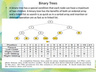
- 52. Binary Trees • A binary tree has a special condition that each node can have a maximum of two children. A binary tree has the benefits of both an ordered array and a linked list as search is as quick as in a sorted array and insertion or deletion operation are as fast as in linked list. 52Neofour.com
- 53. Binary Search Trees • Binary Search tree exhibits a special behavior. A node's left child must have a value less than its parent's value and the node's right child must have a value greater than its parent value. • Programming Example 53Neofour.com
- 54. Heaps • When a collection of objects is organized by importance or priority, we call this priority queue. A heap is defined by two properties. First, it is a complete binary tree, so heaps are nearly always implemented using the array representation. Second, the values stored in a heap are partially ordered. This means that there is a relationship between the values stored at any node and the values of its children. • A max-heap has the property that every node stores a value that is greater than or equal to the value of either of its children. Because the root has a value greater than or equal to its children, which in turn have values greater than or equal to their children, the root store the maximum of all values in the tree. • A min-heap has the property that every node stores a value that is less than or equal to that of its children. Because the root has a value less than or equal to its children, which in turn have values less than or equal to their children, the root stores the minimum of all values in the tree. 54Neofour.com
- 55. Priority Queues • A priority queue is an abstract data type for storing a collection of prioritized elements that supports arbitrary element insertion but supports removal of elements in order of priority, that is, the element with first priority can be removed at any time. • The two fundamental methods of a priority queue P are as follows: – insert(k,x): Insert a value x with key k into P. – removeMin(): Return and remove from P an entry with the smallest key, that is, an entry whose key is less than or equal to that of every other entry in P. • An adaptable priority queue P supports the following methods in addition to those of the priority queue ADT: – remove(e): Remove from P and return entry e. – replaceKey(e,k): Replace with k and return the key of entry e of P; an – error condition occurs if k is invalid (that is, k cannot be – compared with other keys). – replaceValue(e,x): Replace with x and return the value of entry e of P. 55Neofour.com
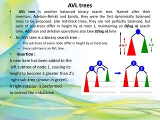
- 56. AVL trees • AVL tree is another balanced binary search tree. Named after their inventors, Adelson-Velskii and Landis, they were the first dynamically balanced trees to be proposed. Like red-black trees, they are not perfectly balanced, but pairs of sub-trees differ in height by at most 1, maintaining an O(log n) search time. Addition and deletion operations also take O(log n) time. • An AVL tree is a binary search tree : – The sub-trees of every node differ in height by at most one. – Every sub-tree is an AVL tree. • Insertion : A new item has been added to the left subtree of node 1, causing its height to become 2 greater than 2's right sub-tree (shown in green). A right-rotation is performed to correct the imbalance 56Neofour.com
- 57. AVL Rotations • To balance itself, an AVL tree may perform the following four kinds of rotations − – Left rotation – Right rotation – Left-Right rotation – Right-Left rotation • The first two rotations are single rotations and the next two rotations are double rotations. To have an unbalanced tree, we at least need a tree of height 2. With this simple tree, let's understand them one by one. • Left Rotation – If a tree becomes unbalanced, when a node is inserted into the right subtree of the right subtree, then we perform a single left rotation. 57Neofour.com
- 58. Right Rotation : AVL tree may become unbalanced, if a node is inserted in the left subtree of the left subtree. The tree then needs a right rotation. Left-Right Rotation : A left-right rotation is a combination of left rotation followed by right rotation. 58Neofour.com AVL Rotations contd. A node has been inserted into the right subtree of the left subtree. This makes C an unbalanced node. These scenarios cause AVL tree to perform left-right rotation. We first perform the left rotation on the left subtree of C. This makes A, the left subtree of B. Node C is still unbalanced, however now, it is because of the left-subtree of the left-subtree. We shall now right-rotate the tree, making B the new root node of this subtree. C now becomes the right subtree of its own left subtree. The tree is now balanced.
- 59. Right-Left Rotation A node has been inserted into the left subtree of the right subtree. This makes A, an unbalanced node with balance factor 2. First, we perform the right rotation along C node, making C the right subtree of its own left subtree B. Now, B becomes the right subtree of A. Node A is still unbalanced because of the right subtree of its right subtree and requires a left rotation. A left rotation is performed by making B the new root node of the subtree. A becomes the left subtree of its right subtree B. The tree is now balanced. 59Neofour.com
- 61. Why AVL TREES Most of the BST operations (e.g., search, max, min, insert, delete.. etc) take O(h) time where h is the height of the BST. The cost of these operations may become O(n) for a skewed Binary tree. If we make sure that height of the tree remains O(Log n) after every insertion and deletion, then we can guarantee an upper bound of O(Log n) for all these operations. The height of an AVL tree is always O(Log n) where n is the number of nodes in the tree. 61Neofour.com
- 62. B Trees (or general m-way search trees) • Search tree called B-Tree in which a node can store more than one value (key) and it can have more than two children. B-Tree was developed in the year of 1972 by Bayer and McCreight with the name Height Balanced m-way Search Tree. Later it was named as B-Tree. B-Tree is a self-balanced search tree with multiple keys in every node and more than two children for every node. • B-Tree of Order m has the following properties... • Property #1 - All the leaf nodes must be at same level. • Property #2 - All nodes except root must have at least [m/2]-1 keys and maximum of m-1 keys. • Property #3 - All non leaf nodes except root (i.e. all internal nodes) must have at least m/2 children. • Property #4 - If the root node is a non leaf node, then it must have at least 2 children. • Property #5 - A non leaf node with n-1 keys must have n number of children. • Property #6 - All the key values within a node must be in Ascending Order. • For example, B-Tree of Order 4 contains maximum 3 key values in a node and maximum 4 children for a node. 62Neofour.com
- 63. B Trees (or general m-way search trees) contd. • The following operations are performed on a B-Tree... Search, Insertion , Deletion • In B-Tree also search process starts from the root node but every time we make n-way decision where n is the total number of children that node has. In a B-Ttree, the search operation is performed with O(log n) time complexity. The search operation is performed as follows... – Step 1: Read the search element from the user – Step 2: Compare, the search element with first key value of root node in the tree. – Step 3: If both are matching, then display "Given node found!!!" and terminate the function – Step 4: If both are not matching, then check whether search element is smaller or larger than that key value. – Step 5: If search element is smaller, then continue the search process in left subtree. – Step 6: If search element is larger, then compare with next key value in the same node and repeat step 3, 4, 5 and 6 until we found exact match or comparison completed with last key value in a leaf node. – Step 7: If we completed with last key value in a leaf node, then display "Element is not found" and terminate the function. 63Neofour.com
- 64. B tree contd. • Insertion Operation in B-Tree : In a B-Tree, the new element must be added only at leaf node. That means, always the new key Value is attached to leaf node only. The insertion operation is performed as follows... – Step 1: Check whether tree is Empty. – Step 2: If tree is Empty, then create a new node with new key value and insert into the tree as a root node. – Step 3: If tree is Not Empty, then find a leaf node to which the new key value cab be added using Binary Search Tree logic. – Step 4: If that leaf node has an empty position, then add the new key value to that leaf node by maintaining ascending order of key value within the node. – Step 5: If that leaf node is already full, then split that leaf node by sending middle value to its parent node. Repeat the same until sending value is fixed into a node. – Step 6: If the splitting is occurring to the root node, then the middle value becomes new root node for the tree and the height of the tree is increased by one. • Programming example 64Neofour.com
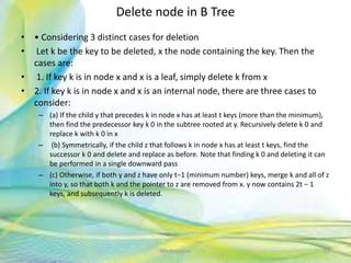
- 65. Delete node in B Tree • • Considering 3 distinct cases for deletion • Let k be the key to be deleted, x the node containing the key. Then the cases are: • 1. If key k is in node x and x is a leaf, simply delete k from x • 2. If key k is in node x and x is an internal node, there are three cases to consider: – (a) If the child y that precedes k in node x has at least t keys (more than the minimum), then find the predecessor key k 0 in the subtree rooted at y. Recursively delete k 0 and replace k with k 0 in x – (b) Symmetrically, if the child z that follows k in node x has at least t keys, find the successor k 0 and delete and replace as before. Note that finding k 0 and deleting it can be performed in a single downward pass – (c) Otherwise, if both y and z have only t−1 (minimum number) keys, merge k and all of z into y, so that both k and the pointer to z are removed from x. y now contains 2t − 1 keys, and subsequently k is deleted. 65Neofour.com
- 66. Delete node in B Tree contd. • 3. If key k is not present in an internal node x, determine the root of the appropriate subtree that must contain k. If the root has only t − 1 keys, execute either of the following two cases to ensure that we descend to a node containing at least t keys. Finally, recurse to the appropriate child of x (a) • If the root has only t−1 keys but has a sibling with t keys, give the root an extra key by moving a key from x to the root, moving a key from the roots immediate left or right sibling up into x, and moving the appropriate child from the sibling to x • (b) If the root and all of its siblings have t − 1 keys, merge the root with one sibling. This involves moving a key down from x into the new merged node to become the median key for that node. 66Neofour.com
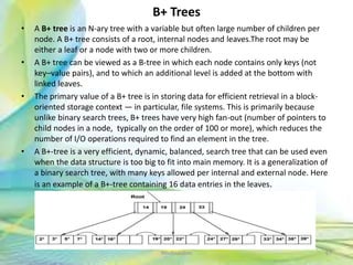
- 67. B+ Trees • A B+ tree is an N-ary tree with a variable but often large number of children per node. A B+ tree consists of a root, internal nodes and leaves.The root may be either a leaf or a node with two or more children. • A B+ tree can be viewed as a B-tree in which each node contains only keys (not key–value pairs), and to which an additional level is added at the bottom with linked leaves. • The primary value of a B+ tree is in storing data for efficient retrieval in a block- oriented storage context — in particular, file systems. This is primarily because unlike binary search trees, B+ trees have very high fan-out (number of pointers to child nodes in a node, typically on the order of 100 or more), which reduces the number of I/O operations required to find an element in the tree. • A B+-tree is a very efficient, dynamic, balanced, search tree that can be used even when the data structure is too big to fit into main memory. It is a generalization of a binary search tree, with many keys allowed per internal and external node. Here is an example of a B+-tree containing 16 data entries in the leaves. 67Neofour.com
- 68. 2-3 Trees • A 2–3 tree is a tree data structure, where every node with children (internal node) has either two children (2-node) and one data element or three children (3-nodes) and two data elements. According to Knuth, "a B-tree of order 3 is a 2-3 tree." Nodes on the outside of the tree (leaf nodes) have no children and one or two data elements. 2−3 trees were invented by John Hopcroft in 1970. • Here are the properties of a 2-3 tree: – Each node has either one value or two value – A node with one value is either a leaf node or has exactly two children (non-null). Values in left subtree < value in node < values in right subtree – A node with two values is either a leaf node or has exactly three children (non-null). Values in left subtree < first value in node < values in middle subtree < second value in node < value in right subtree. – All leaf nodes are at the same level of the tree 68Neofour.com
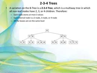
- 69. 2-3-4 Trees • A variation on the B-Tree is a 2-3-4 Tree, which is a multiway tree in which all non-leaf nodes have 2, 3, or 4 children. Therefore: – Each node stores at most 3 values – Each internal node is a 2-node, 3-node, or 4-node – All the leaves are on the same level 69Neofour.com
- 70. Red Black Trees • This type of representation results in a Red-Black Tree, which is a binary search tree with two types of links/nodes, red and black, that satisfy the following properties: – black condition - every path from the root to a leaf node has the same number of black links/nodes – red condition - no path from the root a leaf node has two or more consecutive red links/nodes (ie. every red node will have a black parent) – the root is always black. • The nodes in a Red-Black Tree might be represented as follows: • template <class T> class RedBlackNode {public: ... private: T data; • char color; // 'R' if the incoming link is red, 'B' if the incoming link is black • RedBlackNode *leftChild, *rightChild;}; 70Neofour.com
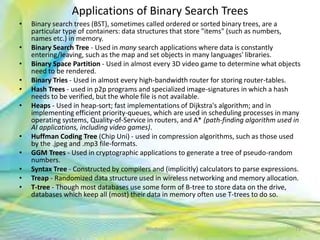
- 71. Applications of Binary Search Trees • Binary search trees (BST), sometimes called ordered or sorted binary trees, are a particular type of containers: data structures that store "items" (such as numbers, names etc.) in memory. • Binary Search Tree - Used in many search applications where data is constantly entering/leaving, such as the map and set objects in many languages' libraries. • Binary Space Partition - Used in almost every 3D video game to determine what objects need to be rendered. • Binary Tries - Used in almost every high-bandwidth router for storing router-tables. • Hash Trees - used in p2p programs and specialized image-signatures in which a hash needs to be verified, but the whole file is not available. • Heaps - Used in heap-sort; fast implementations of Dijkstra's algorithm; and in implementing efficient priority-queues, which are used in scheduling processes in many operating systems, Quality-of-Service in routers, and A* (path-finding algorithm used in AI applications, including video games). • Huffman Coding Tree (Chip Uni) - used in compression algorithms, such as those used by the .jpeg and .mp3 file-formats. • GGM Trees - Used in cryptographic applications to generate a tree of pseudo-random numbers. • Syntax Tree - Constructed by compilers and (implicitly) calculators to parse expressions. • Treap - Randomized data structure used in wireless networking and memory allocation. • T-tree - Though most databases use some form of B-tree to store data on the drive, databases which keep all (most) their data in memory often use T-trees to do so. 71Neofour.com
- 72. MAP • A map is an abstract data type designed to efficiently store and retrieve values based upon a uniquely identifying search key for each. Specifically, a map stores keyvalue pairs (k,v), which we call entries, where k is the key and v is its corresponding value. Keys are required to be unique, so that the association of keys to values defines a mapping. – The key of a page is its URL (e.g., http://neofour.com/ ) and its value is the page content. – Since a map stores a collection of objects, it should be viewed as a collection of – key-value pairs. • As an ADT, a map M supports the following methods: – size( ): Returns the number of entries in M. – isEmpty( ): Returns a boolean indicating whether M is empty. – get(k): Returns the value v associated with key k, if such an entry exists; otherwise returns null. – put(k, v): If M does not have an entry with key equal to k, then adds entry (k,v) to M and returns null; else, replaces with v the existing value of the entry with key equal to k and returns the old value. – remove(k): Removes from M the entry with key equal to k, and returns its value; if M has no such entry, then returns null. – keySet( ): Returns an iterable collection containing all the keys stored inM. – values( ): Returns an iterable collection containing all the values of entries stored in M (with repetition if multiple keys map to the same value). – entrySet( ): Returns an iterable collection containing all the key-value entries in M. 72Neofour.com
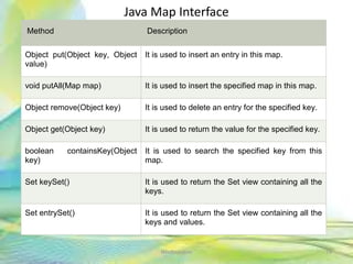
- 74. Java Map Interface 74Neofour.com Method Description Object put(Object key, Object value) It is used to insert an entry in this map. void putAll(Map map) It is used to insert the specified map in this map. Object remove(Object key) It is used to delete an entry for the specified key. Object get(Object key) It is used to return the value for the specified key. boolean containsKey(Object key) It is used to search the specified key from this map. Set keySet() It is used to return the Set view containing all the keys. Set entrySet() It is used to return the Set view containing all the keys and values.
- 75. Java Map Interface program import java.util.*; public class MapInterfaceExample { public static void main(String args[] ) { HashMap <Integer,String> map = new HashMap <Integer,String> (); map.put(100,"Amit"); map.put(101,"Vijay"); map.put(102,"Rahul"); map.put(101, "narayan"); for(HashMap.Entry m:map.entrySet()){ System.out.println(m.getKey()+" "+m.getValue()); } } } 75Neofour.com
- 76. HASH TABLE • Hashing is a technique that is used to uniquely identify a specific object from a group of similar objects. Some examples of how hashing is used in our lives include: – In universities, each student is assigned a unique roll number that can be used to retrieve information about them. – In libraries, each book is assigned a unique number that can be used to determine information about the book, such as its exact position in the library or the users it has been issued to etc. • In hashing, large keys are converted into small keys by using hash functions. The values are then stored in a data structure called hash table. The idea of hashing is to distribute entries (key/value pairs) uniformly across an array. Each element is assigned a key (converted key). By using that key you can access the element in O(1) time. Using the key, the algorithm (hash function) computes an index that suggests where an entry can be found or inserted. • Hashing is implemented in two steps: – An element is converted into an integer by using a hash function. This element can be used as an index to store the original element, which falls into the hash table. – The element is stored in the hash table where it can be quickly retrieved using hashed key. – hash = hashfunc(key) , index = hash % array_size 76Neofour.com
- 77. Hash Function • A hash function is any function that can be used to map a data set of an arbitrary size to a data set of a fixed size, which falls into the hash table. The values returned by a hash function are called hash values, hash codes, hash sums, or simply hashes. – To achieve a good hashing mechanism, It is important to have a good hash function with the following basic requirements: – Easy to compute: It should be easy to compute and must not become an algorithm in itself. – Uniform distribution: It should provide a uniform distribution across the hash table and should not result in clustering. – Less collisions: Collisions occur when pairs of elements are mapped to the same hash value. These should be avoided. • Note: Irrespective of how good a hash function is, collisions are bound to occur. Therefore, to maintain the performance of a hash table, it is important to manage collisions through various collision resolution techniques. • A hash table is a data structure that is used to store keys/value pairs. It uses a hash function to compute an index into an array in which an element will be inserted or searched. By using a good hash function, hashing can work well. Under reasonable assumptions, the average time required to search for an element in a hash table is O(1). 77Neofour.com
- 78. Graphs • A graph is made up of a set of vertices and edges that form connections between vertices. If the edges are directed, the graph is sometimes called a digraph. Graphs can be used to model data where we are interested in connections and relationships between data. • Graph is a data structure that consists of following two components: 1. A finite set of vertices also called as nodes. 2. A finite set of ordered pair of the form (u, v) called as edge. The pair is ordered because (u, v) is not same as (v, u) in case of directed graph(di-graph). The pair of form (u, v) indicates that there is an edge from vertex u to vertex v. The edges may contain weight/value/cost. • Graphs are used to represent many real life applications: Graphs are used to represent networks. The networks may include paths in a city or telephone network or circuit network. Graphs are also used in social networks like linkedIn, facebook. For example, in facebook, each person is represented with a vertex(or node). Each node is a structure and contains information like person id, name, gender and locale. 78Neofour.com
- 79. Graph Contd • Following two are the most commonly used representations of graph. 1. Adjacency Matrix 2. Adjacency List There are other representations also like, Incidence Matrix and Incidence List. The choice of the graph representation is situation specific. It totally depends on the type of operations to be performed and ease of use. • Graph Terminology – Adjacent - Given two nodes A and B. B is adjacent to A if there is a connection from A to B. In a digraph if B is adjacent to A, it doesn't mean that A is automatically adjacent to B. – edge weight/edge cost - a value associated with a connection between two nodes – path - a ordered sequence of vertices where a connection must exist between consecutive pairs in the sequence. – Simple path - every vertex in path is distinct – Path length number of edges in a path – cycle - a path where the starting and ending node is the same – strongly connected - If there exists some path from every vertex to every other vertex, the graph is strongly connected. – weakly connect - if we take away the direction of the edges and there exists a path from every node to every other node, the digraph is weakly connected. – An edge (u,v) is said to be directed from u to v if the pair (u,v) is ordered, with u preceding v. An edge (u,v) is said to be undirected if the pair (u,v) is not ordered. 79Neofour.com
- 80. Graph Representation • Adjacency Matrix is a 2D array of size V x V where V is the number of vertices in a graph. Let the 2D array be adj[][], a slot adj[i][j] = 1 indicates that there is an edge from vertex i to vertex j. Adjacency matrix for undirected graph is always symmetric. Adjacency Matrix is also used to represent weighted graphs. If adj[i][j] = w, then there is an edge from vertex i to vertex j with weight w. • The adjacency matrix for the graph is: – Pros: Representation is easier to implement and follow. Removing an edge takes O(1) time. Queries like whether there is an edge from vertex ‘u’ to vertex ‘v’ are efficient and can be done O(1). – Cons: Consumes more space O(V^2). Even if the graph is sparse(contains less number of edges), it consumes the same space. Adding a vertex is O(V^2) time. • Adjacency List : An array of linked lists is used. Size of the array is equal to number of vertices. Let the array be array[]. An entry array[i] represents the linked list of vertices adjacent to the ith vertex. This representation can also be used to represent a weighted graph. The weights of edges can be stored in nodes of linked lists. Following is adjacency list representation of the above graph. 80Neofour.com
- 81. Graph ADT • numVertices( ): Returns the number of vertices of the graph. • vertices( ): Returns an iteration of all the vertices of the graph. • numEdges( ): Returns the number of edges of the graph. • edges( ): Returns an iteration of all the edges of the graph. • getEdge(u, v): Returns the edge from vertex u to vertex v, if one exists; otherwise return null. For an undirected graph, there is no difference between getEdge(u, v) and getEdge(v, u). • endVertices(e): Returns an array containing the two endpoint vertices of edge e. If the graph is directed, the first vertex is the origin and the second is the destination. • opposite(v, e): For edge e incident to vertex v, returns the other vertex of the edge; an error occurs if e is not incident to v. • outDegree(v): Returns the number of outgoing edges from vertex v. • inDegree(v): Returns the number of incoming edges to vertex v. For an undirected graph, this returns the same value as does outDegree(v). • outgoingEdges(v): Returns an iteration of all outgoing edges from vertex v. • incomingEdges(v): Returns an iteration of all incoming edges to vertex v. For an undirected graph, this returns the same collection as does outgoingEdges(v). • insertVertex(x): Creates and returns a new Vertex storing element x. • insertEdge(u, v, x): Creates and returns a new Edge from vertex u to vertex v, storing element x; an error occurs if there already exists an edge from u to v. • removeVertex(v): Removes vertex v and all its incident edges from the graph. • removeEdge(e): Removes edge e from the graph. 81Neofour.com
- 82. Graph Contd. • Traversing a Graph : Whether it is possible to traverse a graph from one vertex to another is determined by how a graph is connected. Connectivity is a basic concept in Graph Theory. Connectivity defines whether a graph is connected or disconnected. It has subtopics based on edge and vertex, known as edge connectivity and vertex connectivity. Let us discuss them in detail. • Connectivity : A graph is said to be connected if there is a path between every pair of vertex. From every vertex to any other vertex, there should be some path to traverse. That is called the connectivity of a graph. A graph with multiple disconnected vertices and edges is said to be disconnected. • Cut Vertex : Let ‘G’ be a connected graph. A vertex V ∈ G is called a cut vertex of ‘G’, if ‘G-V’ (Delete ‘V’ from ‘G’) results in a disconnected graph. Removing a cut vertex from a graph breaks it in to two or more graphs. • Cut Edge (Bridge) : Let ‘G’ be a connected graph. An edge ‘e’ ∈ G is called a cut edge if ‘G-e’ results in a disconnected graph. If removing an edge in a graph results in to two or more graphs, then that edge is called a Cut Edge. • Cut Set of a Graph : Let ‘G’= (V, E) be a connected graph. A subset E’ of E is called a cut set of G if deletion of all the edges of E’ from G makes G disconnect. If deleting a certain number of edges from a graph makes it disconnected, then those deleted edges are called the cut set of the graph. • Edge Connectivity : Let ‘G’ be a connected graph. The minimum number of edges whose removal makes ‘G’ disconnected is called edge connectivity of G. Notation − λ(G) . In other words, the number of edges in a smallest cut set of G is called the edge connectivity of G. 82Neofour.com
- 83. Graph Contd. • Vertex Connectivity : Let ‘G’ be a connected graph. The minimum number of vertices whose removal makes ‘G’ either disconnected or reduces ‘G’ in to a trivial graph is called its vertex connectivity. Notation − K(G). • Line Covering : Let G = (V, E) be a graph. A subset C(E) is called a line covering of G if every vertex of G is incident with at least one edge in C, i.e., deg(V) ≥ 1 ∀ V ∈ G because each vertex is connected with another vertex by an edge. Hence it has a minimum degree of 1. • Minimal Line Covering : A line covering C of a graph G is said to be minimal if no edge can be deleted from C. • Vertex Coloring : Vertex coloring is an assignment of colors to the vertices of a graph ‘G’ such that no two adjacent vertices have the same color. Simply put, no two vertices of an edge should be of the same color. • Chromatic Number : The minimum number of colors required for vertex coloring of graph ‘G’ is called as the chromatic number of G, denoted by X(G). χ(G) = 1 if and only if •'G•' is a null graph. If 'G' is not a null graph, then χ(G) ≥ 2. • Note − A graph ‘G’ is said to be n-coverable if there is a vertex coloring that uses at most n colors, i.e., X(G) ≤ n. 83Neofour.com
- 84. Graph Contd. • Region Coloring : Region coloring is an assignment of colors to the regions of a planar graph such that no two adjacent regions have the same color. Two regions are said to be adjacent if they have a common edge. • Applications of Graph Coloring Graph coloring is one of the most important concepts in graph theory. It is used in many real- time applications of computer science such as − • Clustering Data mining Image capturing Image segmentation • Networking Resource allocation Processes scheduling 84Neofour.com
- 85. Graph Contd. • Isomorphic Graphs : Two graphs G1 and G2 are said to be isomorphic if – Their number of components (vertices and edges) are same. – Their edge connectivity is retained. • Planar Graphs: A graph ‘G’ is said to be planar if it can be drawn on a plane or a sphere so that no two edges cross each other at a non-vertex point. 85Neofour.com
- 86. Graph Contd. • Regions : Every planar graph divides the plane into connected areas called regions. • Degree of a bounded region r = deg(r) = Number of edges enclosing the regions r. deg(1) = 3 , deg(2) = 4 , deg(3) = 4, deg(4) = 3, deg(5) = 8 • In planar graphs, the following properties hold good − – 1. In a planar graph with ‘n’ vertices, sum of degrees of all the vertices is n∑i=1 deg(Vi) = 2|E| – 2. According to Sum of Degrees of Regions Theorem, in a planar graph with ‘n’ regions, Sum of degrees of regions is n∑i=1 deg(ri) = 2|E| 86Neofour.com
- 87. Euler’s Path : An Euler’s path contains each edge of ‘G’ exactly once and each vertex of ‘G’ at least once. A connected graph G is said to be traversable if it contains an Euler’s path (d-c-a-b-d-e) . Euler’s Circuit : In an Euler’s path, if the starting vertex is same as its ending vertex, then it is called an Euler’s circuit. = a-b-c-d-a-g-f-e-c-a. Euler’s Circuit Theorem : A connected graph ‘G’ is traversable if and only if the number of vertices with odd degree in G is exactly 2 or 0. A connected graph G can contain an Euler’s path, but not an Euler’s circuit, if it has exactly two vertices with an odd degree. Note − This Euler path begins with a vertex of odd degree and ends with the other vertex of odd degree Euler’s Path − b-e-a-b-d-c-a is not an Euler’s circuit, but it is an Euler’s path. Clearly it has exactly 2 odd degree vertices. Note − In a connected graph G, if the number of vertices with odd degree = 0, then Euler’s circuit exists. 87Neofour.com
- 88. Graph Contd. • Hamiltonian Graph A connected graph G is said to be a Hamiltonian graph, if there exists a cycle which contains all the vertices of G. Every cycle is a circuit but a circuit may contain multiple cycles. Such a cycle is called a Hamiltonian cycle of G. • Hamiltonian Path A connected graph is said to be Hamiltonian if it contains each vertex of G exactly once. Such a path is called a Hamiltonian path. • Hamiltonian Path − e-d-b-a-c. • Graph traversal : (Also known as graph search) refers to the process of visiting (checking and/or updating) each vertex in a graph. Such traversals are classified by the order in which the vertices are visited. Tree traversal is a special case of graph traversal. Unlike tree traversal, graph traversal may require that some vertices be visited more than once, since it is not necessarily known before transitioning to a vertex that it has already been explored. As graphs become more dense, this redundancy becomes more prevalent, causing computation time to increase; as graphs become more sparse, the opposite holds true. 88Neofour.com
- 89. Graph Traversal Depth-first search :A depth-first search (DFS) is an algorithm for traversing a finite graph. DFS visits the child vertices before visiting the sibling vertices; that is, it traverses the depth of any particular path before exploring its breadth. A stack (often the program's call stack via recursion) is generally used when implementing the algorithm. • Input: A graph G and a vertex v of G. • Output: A labeling of the edges in the connected component of v as discovery edges and back edges. 1 procedure DFS(G, v): 2 label v as explored 3 for all edges e in G.incidentEdges(v) do 4 if edge e is unexplored then 5 w ← G.adjacentVertex(v, e) 6 if vertex w is unexplored then 7 label e as a discovered edge 8 recursively call DFS(G, w) 9 else 10 label e as a back edge 89Neofour.com
- 90. Graph Traversal A breadth-first search (BFS) is another technique for traversing a finite graph. BFS visits the neighbor vertices before visiting the child vertices, and a queue is used in the search process. This algorithm is often used to find the shortest path from one vertex to another. Input: A graph G and a vertex v of G. Output: The closest vertex to v satisfying some conditions, or null if no such vertex exists. 1 procedure BFS(G, v): 2 create a queue Q 3 enqueue v onto Q 4 mark v 5 while Q is not empty: 6 t ← Q.dequeue() 7 if t is what we are looking for: 8 return t 9 for all edges e in G.adjacentEdges(t) do 12 o ← G.adjacentVertex(t, e) 13 if o is not marked: 14 mark o 15 enqueue o onto Q 16 return null 90Neofour.com
- 91. Application of Graph • Facebook: Each user is represented as a vertex and two people are friends when there is an edge between two vertices. Similarly friend suggestion also uses graph theory concept. • Google Maps: Various locations are represented as vertices and the roads are represented as edges and graph theory is used to find shortest path between two nodes. • Recommendations on e-commerce websites: The “Recommendations for you” section on various e-commerce websites uses graph theory to recommend items of similar type to user’s choice. • Graph theory is also used to study molecules in chemistry and physics. • Social network graphs: to tweet or not to tweet. Graphs that represent who knows whom, who communicates with whom, who influences whom or other relationships in social structures. An example is the twitter graph of who follows whom. These can be used to determine how information flows, how topics become hot, how communities develop, or even who might be a good match for who, or is that whom. • Transportation networks. In road networks vertices are intersections and edges are the road segments between them, and for public transportation networks vertices are stops and edges are the links between them. Such networks are used by many map programs such as Google maps, Bing maps and now Apple IOS 6 maps (well perhaps without the public transport) to find the best routes between locations. They are also used for studying traffic patterns, traffic light timings, and many aspects of transportation. • Utility graphs. The power grid, the Internet, and the water network are all examples of graphs where vertices represent connection points, and edges the wires or pipes between them. Analyzing properties of these graphs is very important in understanding the reliability of such utilities under failure or attack, or in minimizing the costs to build infrastructure that matches required demands. • Document link graphs. The best known example is the link graph of the web, where each web page is a vertex, and each hyperlink a directed edge. Link graphs are used, for example, to analyze relevance of web pages, the best sources of information, and good link sites. 91Neofour.com
- 92. Application of Graph • 5. Protein-protein interactions graphs. Vertices represent proteins and edges represent interactions between them that carry out some biological function in the cell. These graphs can be used, for example, to study molecular pathways—chains of molecular interactions in a cellular process. Humans have over 120K proteins with millions of interactions among them. • 6. Network packet traffic graphs. Vertices are IP (Internet protocol) addresses and edges are the packets that flow between them. Such graphs are used for analyzing network security, studying the spread of worms, and tracking criminal or non-criminal activity. • 7. Scene graphs. In graphics and computer games scene graphs represent the logical or special relationships between objects in a scene. Such graphs are very important in the computer games industry. • 8. Finite element meshes. In engineering many simulations of physical systems, such as the flow of air over a car or airplane wing, the spread of earthquakes through the ground, or the structural vibrations of a building, involve partitioning space into discrete elements. The elements along with the connections between adjacent elements forms a graph that is called a finite element mesh. • 9. Robot planning. Vertices represent states the robot can be in and the edges the possible transitions between the states. This requires approximating continuous motion as a sequence of discrete steps. Such graph plans are used, for example, in planning paths for autonomous vehicles. • 10. Neural networks. Vertices represent neurons and edges the synapses between them. Neural networks are used to understand how our brain works and how connections change when we learn. The human brain has about 10^11 neurons and close to 10^15 synapses 92Neofour.com
- 93. Application of Graph • 11. Graphs in quantum field theory. Vertices represent states of a quantum system and the edges the transitions between them. The graphs can be used to analyze path integrals and summing these up generates a quantum amplitude (yes, I have no idea what that means). • 12. Semantic networks. Vertices represent words or concepts and edges represent the relationships among the words or concepts. These have been used in various models of how humans organize their knowledge, and how machines might simulate such an organization. • 13. Graphs in epidemiology. Vertices represent individuals and directed edges the transfer of an infectious disease from one individual to another. Analyzing such graphs has become an important component in understanding and controlling the spread of diseases. • 14. Graphs in compilers. Graphs are used extensively in compilers. They can be used for type inference, for so called data flow analysis, register allocation and many other purposes. They are also used in specialized compilers, such as query optimization in database languages. • 15. Constraint graphs. Graphs are often used to represent constraints among items. For example the GSM network for cell phones consists of a collection of overlapping cells. Any pair of cells that overlap must operate at different frequencies. These constraints can be modeled as a graph where the cells are vertices and edges are placed between cells that overlap. • 16. Dependence graphs. Graphs can be used to represent dependences or precedences among items. Such graphs are often used in large projects in laying out what components rely on other components and used to minimize the total time or cost to completion while abiding by the dependences. 93Neofour.com
- 94. Graph Contd. • Spanning Trees : A spanning tree T of an undirected graph G is a sub graph that includes all of the vertices of G. • Circuit Rank : Let ‘G’ be a connected graph with ‘n’ vertices and ‘m’ edges. A spanning tree ‘T’ of G contains (n-1) edges. Therefore, the number of edges you need to delete from ‘G’ in order to get a spanning tree = m-(n-1), which is called the circuit rank of G. This formula is true, because in a spanning tree you need to have ‘n-1’ edges. Out of ‘m’ edges, you need to keep ‘n–1’ edges in the graph. Hence, deleting ‘n–1’ edges from ‘m’ gives the edges to be removed from the graph in order to get a spanning tree, which should not form a cycle. For the graph given in the below example, We have m=7 edges and n=5 vertices. Then the circuit rank is G = m – (n – 1) = 7 – (5 – 1) = 3 94Neofour.com
- 95. Graph Contd. • Kirchoff’s Theorem : Kirchoff’s theorem is useful in finding the number of spanning trees that can be formed from a connected graph. 95Neofour.com
- 96. Complexity Theory Over the course we have considered many different problems, data structures and algorithms. Aside from knowing what good solutions are to common problems, it is also useful to understand how computer algorithms are classified according to its complexity. This section of the notes looks at complexity theory. • Undecidable Problems : Some problems like the halting problems are undecidable. The halting problem is described simply as this... is it possible to write a program that will determine if any program has an infinite loop. • P class Problems : Any problem that can be solved in polynomial time is considered to be class P. For example, sorting is a class P problem because we have several algorithms who's solution is in polynomial time. • NP class Problems : When we talk about "hard" problems then, we aren't talking about the impossible ones like the halting problem. We are instead talking about problems where its possible to find a solution, just that no good solution is currently known. The NP, in NP class stands for non-deterministic polynomial time. • NP-Complete Problems : A subset of the NP class problems is the NP- complete problems. NP-complete problems are problems where any problem in NP can be polynomially reduced to it. That is, a problem is considered to be NP-complete if it is able to provide a mapping from any NP class problem to it and back. • NP-Hard : A problem is NP-Hard if any problem NP problem can be mapped to it and back in polynomial time. However, the problem does not need to be NP... that is a solution does not need to be verified in polynomial time 96Neofour.com
- 97. Neofour.com 97
Editor's Notes
- #56: Suppose a certain flight is fully booked an hour prior to departure. Because of the possibility of cancellations, the airline maintains a priority queue of standby passengers hoping to get a seat. The priority of each standby passenger is determined by the airline taking into account the fare paid, the frequent-flyer status, and the time that the passenger is inserted into the priority queue. A standby passenger reference is inserted into the priority queue with an insert operation as soon as he or she requests to fly standby. Shortly before the flight departure, if seats become available (for example, due to no-shows or last-minute cancellations), the airline removes a standby passenger with first priority from the priority queue, using aremoveMin operation and lets this person board. This process is then repeated until all available seats have been filled or the priority queue becomes empty.