Data Structure and algorithms for software

UNIT -3
Sorting and Searching
1

Syllabus
• Insertion,
• Selection,
• Bubble sort methods,
• Divider and conquer:
• Quick sort,
• Merge Sort,
• Shell short & Radix sort,
• Comparison of various sorting techniques.
• Searching Techniques: Sequential search, Binary search,
Comparison trees, Performance Comparison of searching
algorithms,
• Hashing: Hash Function- Open and Closed Hashing, Hash
collisions, Rehashing techniques, Extendible hashing.
2

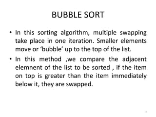
BUBBLE SORT
• In this sorting algorithm, multiple swapping
take place in one iteration. Smaller elements
move or ‘bubble’ up to the top of the list.
• In this method ,we compare the adjacent
elemnent of the list to be sorted , if the item
on top is greater than the item immediately
below it, they are swapped.
3

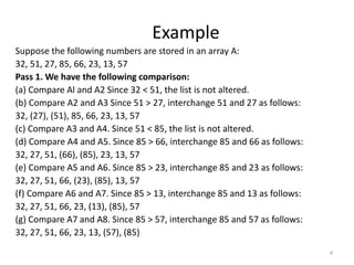
Example
Suppose the following numbers are stored in an array A:
32, 51, 27, 85, 66, 23, 13, 57
Pass 1. We have the following comparison:
(a) Compare Al and A2 Since 32 < 51, the list is not altered.
(b) Compare A2 and A3 Since 51 > 27, interchange 51 and 27 as follows:
32, (27), (51), 85, 66, 23, 13, 57
(c) Compare A3 and A4. Since 51 < 85, the list is not altered.
(d) Compare A4 and A5. Since 85 > 66, interchange 85 and 66 as follows:
32, 27, 51, (66), (85), 23, 13, 57
(e) Compare A5 and A6. Since 85 > 23, interchange 85 and 23 as follows:
32, 27, 51, 66, (23), (85), 13, 57
(f) Compare A6 and A7. Since 85 > 13, interchange 85 and 13 as follows:
32, 27, 51, 66, 23, (13), (85), 57
(g) Compare A7 and A8. Since 85 > 57, interchange 85 and 57 as follows:
32, 27, 51, 66, 23, 13, (57), (85)
4

• At the end of Pass 2, the second largest number, 66, has moved its
way down to the next-to-last position.
27, 33, 51, 23, 13, 57, 66, 85
• At the end of Pass 3, the third largest number, 57, has moved its way
down to its position in the list.
27, 33, 23, 13, 51, 57, 66, 85
• At the end of Pass 4, the fourth largest number, 51, has moved its
way down to its position in the list.
27, 23, 13, 33, 51, 57, 66, 85
• At the end of Pass 5, the fifth largest number, 33, has moved its way
23, 13, 27, 33, 51, 57, 66, 85
• At the end of Pass 6, the sixth largest number, 27, has moved its way
13, 23, 27, 33, 51, 57, 66, 85
• At the end of Pass 7 (last pass), the seventh largest number, 23, has
moved its way down to its position in the list.
13, 23, 27, 33, 51, 57, 66, 85
5

BUBBLE SORT
Algorithm: (Bubble Sort) BUBBLE (A, N)
1. Repeat Steps 2 and 3 for K = 1 to N-1.
2. Set PTR := 1. [Initializes pass pointer PTR.]
3. Repeat while PTR ≤ N – K.
a. If A [PTR] > A[PTR+1], then:
Interchange A[PTR] & A[PTR+1].
[End of IF structure.]
b. Set PTR := PTR + 1.
[End of While loop.]
[End of Step 1 loop.]
4. Exit.
6

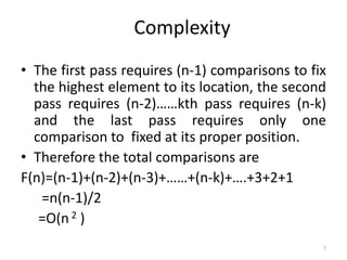
Complexity
• The first pass requires (n-1) comparisons to fix
the highest element to its location, the second
pass requires (n-2)……kth pass requires (n-k)
and the last pass requires only one
comparison to fixed at its proper position.
• Therefore the total comparisons are
F(n)=(n-1)+(n-2)+(n-3)+……+(n-k)+….+3+2+1
=n(n-1)/2
=O(n 2 )
7

SELECTION SORT
• In this sorting we find the smallest element
in this list and put it in the first position.
• Then find the second smallest element in
the list and put it in the second position.
And so on.
8

SELECTION SORT
Algorithm: (Selection Sort) SELECTION (A, N)
1. Repeat Steps 2 and 3 for K = 1,2,3,…,N-1.
2. Call MIN(A,K,N,LOC).
3. [Interchange A[K] and A[LOC].]
4. Exit.
10

SELECTION SORT
Procedure: MIN(A, K, N, LOC)
1. Set MIN : = A[K] and LOC:=K.
2. Repeat for J = K+1, K+2,….,N.
If MIN > A[J], then:
Set MIN := A[J] and LOC:=J.
[End of loop.]
3. Return.
11

Complexity of selection sort
• The first pass requires (n-1) comparisons to
find the location loc of smallest element, the
second pass requires (n-2)……kth pass requires
(n-k) and the last pass requires only one
comparison.
F(n)=(n-1)+(n-2)+(n-3)+……+(n-k)+….+3+2+1
=n(n-1)/2
=O(n 2 )
12

INSERTION SORT
• The insertion sort works just like its name
suggest-it inserts each item its proper place in
the final list.
• During the first iteration, the element position
2nd is compared with the element at the 1st
position.
• During the second iteration, the element at
the position 3rd is compared with the element
at the 2nd and 1st positions.
• This process is repeated for all the elements in
the array up to (n-1) iterations.
• This method is widely used by card players.
13

INSERTION SORT
Algorithm: INSERTION(A, N)
1. Repeat Steps 2 to 4 for K = 2,3,…, N.
2. Set TEMP := A[K] and PTR := K – 1.
3. Repeat while TEMP<A[PTR]
(a) Set A[PTR+1] := A[PTR].
(b) Set PTR := PTR – 1.
[End of Loop.]
5. Set A[PTR + 1] := TEMP.
6. Exit
15

Complexity of insertion sort
• The first pass requires 1 comparison, the
second pass requires 2……kth pass requires k
and the last pass requires (n-1) comparisons.
F(n)=1+2+3+……+(n-1)
=n(n-1)/2
=O(n 2 )
16

17
Divide-and-Conquer
• Divide the problem into a number of sub-problems
– Similar sub-problems of smaller size
• Conquer the sub-problems
– Solve the sub-problems recursively
– Sub-problem size small enough  solve the problems in
straightforward manner
• Combine the solutions of the sub-problems
– Obtain the solution for the original problem

QUICK SORT
• Also known as Partition Exchange Sort.
• Works by partitioning the array to be sorted.
• One of the array elements is chosen as a key
value(Pivot element).
• Key element divides the main list into two parts such
that:
– One partition contains elements smaller than the
key value.
– Another partition contains elements larger than the
key value.
18

QUICK SORT
Algorithm: QuickSort (a, l, r)// a=array, l=first index,
r=last index
1. If l<r
2. Call partition(a,l,r)
3. Quicksort(a, l, j-1) // sort the left hand
4. Quicksort(a, j+1,r) // sort the right hand
5. Exit
19

Procedure partition(a,l,r)
P Pivot element
1. p=a[l], i=l, j=r
2. Repeat
repeat i=i+1 until a[i] ≥ p
repeat j=j-1 until a[j] ≤ p
Swap(a[i], a[j])
until i ≥ j
3. Swap (a[i], a[j]) // undo last swap
4. Swap (p,a[j])
5. Return j
20

Example
• 5 3 1 9 8 2 4 7
• P=5
• i=a[l]=5
• J=a[r]=7
• 5 3 1 9 8 2 4 7
21
i j

• 5 3 1 9 8 2 4 7
• Swap(a[i], a[j])
• 5 3 1 4 8 2 9 7
• 5 3 1 4 8 2 9 7
• 5 3 1 4 2 8 9 7
22
i stop j stop
i j
i stop j stop
j
i

• 5 3 1 4 2 8 9 7
• 5 3 1 4 8 2 9 7
• I >J
• Swap (a[i], a[j])
• 5 3 1 4 2 8 9 7
23
i stop
j stop
i
j
j
i

• Swap (p,a[j])
• 2 3 1 4 5 8 9 7
• Here the pivot element 5 come to the proper
position so repeat the same process for left
array and right array.
24

• Worst-case: O(N2)
This happens when the pivot is the smallest (or
the largest) element. Then one of the partitions is
empty, and we repeat recursively the procedure
for N-1 elements.
• Best-case O(NlogN) The best case is when the
pivot is the median of the array, and then the left
and the right part will have same size. There are
log N partitions, and to obtain each partitions we
do N comparisons. Hence the complexity is
O(NlogN)
25
Complexity of Quick sort

26
Merge Sort
• To sort an array A[p . . r]:
• Divide
– Divide the n-element sequence to be sorted into
two subsequences of n/2 elements each
• Conquer
– Sort the subsequences recursively using merge sort
– When the size of the sequences is 1 there is
nothing more to do
• Combine
– Merge the two sorted subsequences

27
Example – n Power of 2
1 2 3 4 5 6 7 8
q = 4
6
2
3
1
7
4
2
5
1 2 3 4
7
4
2
5
5 6 7 8
6
2
3
1
1 2
2
5
3 4
7
4
5 6
3
1
7 8
6
2
1
5
2
2
3
4
4
7 1
6
3
7
2
8
6
5
Divide

28
Example – n Power of 2
1
5
2
2
3
4
4
7 1
6
3
7
2
8
6
5
1 2 3 4 5 6 7 8
7
6
5
4
3
2
2
1
1 2 3 4
7
5
4
2
5 6 7 8
6
3
2
1
1 2
5
2
3 4
7
4
5 6
3
1
7 8
6
2
Conquer
and
Merge

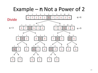
29
Example – n Not a Power of 2
6
2
5
3
7
4
1
6
2
7
4
1 2 3 4 5 6 7 8 9 10 11
q = 6
4
1
6
2
7
4
1 2 3 4 5 6
6
2
5
3
7
7 8 9 10 11
q = 9
q = 3
2
7
4
1 2 3
4
1
6
4 5 6
5
3
7
7 8 9
6
2
10 11
7
4
1 2
2
3
1
6
4 5
4
6
3
7
7 8
5
9
2
10
6
11
4
1
7
2
6
4
1
5
7
7
3
8
Divide

30
Example – n Not a Power of 2
7
7
6
6
5
4
4
3
2
2
1
1 2 3 4 5 6 7 8 9 10 11
7
6
4
4
2
1
1 2 3 4 5 6
7
6
5
3
2
7 8 9 10 11
7
4
2
1 2 3
6
4
1
4 5 6
7
5
3
7 8 9
6
2
10 11
2
3
4
6
5
9
2
10
6
11
4
1
7
2
6
4
1
5
7
7
3
8
7
4
1 2
6
1
4 5
7
3
7 8
Conquer
and
Merge

31
Algorithm
MERGE-SORT(A, p, r)
if p < r Check for base case
then q = (p + r)/2 Divide
MERGE-SORT(A, p, q) Conquer
MERGE-SORT(A, q + 1, r) Conquer
MERGE(A, p, q, r) Combine
1 2 3 4 5 6 7 8
6
2
3
1
7
4
2
5
p r
q

MERGING
• Merging is a process in which two lists are
merged to form a new list.
• Suppose, L is a sorted list with ‘n1’ elements
and R is a sorted list with ‘n2’ elements. The
operation that combines the elements of L
and R into a single sorted list C with ‘n=n1+n2’
elements is called merging.
32

MERGING
Algorithm: MERGE(A,p,q,r )
Compute n1 and n2.
Copy the first n1 elements into L[] and the next n2 elements into R[]. Final result
is stored in c[].
1. [Initialize.] Set i = 1 ,j = 1, k=1
2. [Compare.] Repeat while i ≤ n1 and j ≤ n2.
If L[i] < R[j], then
(a) [Assign element from L to C.]
Set C[k] = L[i].
(b) [Update pointers.] Set k = k + 1 and i = i + 1
Else if L[i] > R[j], then:
(a) [Assign element from R to C.]
Set C[k] = R[j].
(b) [Update pointers.] Set k = k + 1 and j = j + 1
33
1 2 3 4 5 6 7 8
6
3
2
1
7
5
4
2
p r
q
n1 n2

MERGING
Else (a) [Assign element from L to C.]
Set C[k] = L[i].
(b) [Update pointers.] Set k = k + 1, i =i+1, and j = j + 1
[End of If structure.]
[End of loop.]
3. [Assign remaining elements to C.]
If i > n1, then:
Repeat for l=j to n2:
Set C[k] = R[l], k=k+1
Else: Repeat for l=i to n1
Set C[k] = L[l], k=k+1
[End of loop.]
4. Exit.
34

Example
• L = 4 12 13 21 80
• R= 1 41 62 200 412 816
•
35
i j k i≤l1 and j≤l2 C[k]
1 1 1 T 1
1 2 2 T 4
2 2 3 T 12
3 2 4 T 13
4 2 5 T 21
5 2 6 T 41
5 3 7 T 62
5 4 8 T 80
6 4 9 F 200
6 5 10 F 412
6 6 11 F 816

Complexity of merge sort
O(n log n)
36

Radix sort or bucket sort
• Suppose keys are k-digit integers.
• Radix sort uses an array of 10 queues, one for
each digit 0 through 9.
• Each object is placed into the queue whose
index is the least significant digit (the 1’s digit)
of the object’s key.
• Objects are then dequeued from these 10
queues, in order 0 through 9, and put back in
the original queue they’re sorted by the last
digit of the key.
37

Radix sort or bucket sort continued..
• Process is repeated, this time using the 10’s
digit instead of the 1’s digit; values are now
sorted by last two digits of the key.
• Keep repeating, using the 100’s digit, then the
1000’s digit, then the 10000’s digit
• Stop after using the most significant digit.
• Objects are now in order in original container.
38

Algorithm
Radixsort(a, n) // a-array, n-No. of elements
1. Find the largest element of the array.
2. num= total number of digits in the largest number
3. digit=num
4. Repeat Steps 5 to 6 for K = 1 to num
5. Initialize buckets(0 to 9)
For i=1 to n
set num= obtain digit number k of a[i]
put a[i] in bucket number digit
[end of for loop]
6. Combine all numbers from the bucket in order
7. Exit
40

Complexity
O(nk)
where, n number of elements
K the maximum number of digits in each number
41

Shell sort
• Invented by Donald Shell in 1959.
• It moves data items by exchanges. It begins by comparing
items a distance “d” apart. In each pass the value of d is
decreased usually;
d i+1 = (di +1)/2
• In every pass, each item is compared with the one located d
positions further in the vector of items. If the higher item has a
lower value, an exchange is made.
• The sort continues by comparing the next item in the vector
with an item d locations away. If an exchange is again
indicated, it is made and the comparison is tried again with the
next entry. This proceeds until no lower items remain.
42

Example 2
• Sort: 18 32 12 5 38 33 16 2
8 Numbers to be sorted, Shell’s increment will be floor(n/2)
* floor(8/2)  floor(4) = 4
increment 4: 1 2 3 4
18 32 12 5 38 33 16 2
(visualize underlining)
Step 1) Only look at 18 and 38 and sort in order ;
18 and 38 stays at its current position because they are in order.
2 and 5 need to be switched to be in order. 44

Example 2 (con’t)
• Sort: 18 32 12 5 38 33 16 2
Resulting numbers after increment 4 pass:
18 32 12 2 38 33 16 5
* floor(4/2)  floor(2) = 2
increment 2: 1 2
18 32 12 2 38 33 16 5
Step 1) Look at 18, 12, 38, 16 and sort them in their appropriate location:
12 38 16 2 18 33 38 5
Step 2) Look at 32, 2, 33, 5 and sort them in their appropriate location:
12 2 16 5 18 32 38 33
45

Example 2 (con’t)
• Sort: 18 32 12 5 38 33 16 2
* floor(2/2)  floor(1) = 1
increment 1: 1
12 2 16 5 18 32 38 33
2 5 12 16 18 32 33 38
The last increment or phase of Shellsort is basically an Insertion
Sort algorithm.
46

Algorithm
Shell(A,N)
for( Increment = N/2; Increment > 0; Increment /= 2 )
{
for( i = Increment; i < N; i++ )
{
Tmp = A[ i ];
for( j = i; j >= Increment && A[ j - Increment ] > Tmp ; j -= Increment )
{
A[ j ] = A[ j - Increment ];
}
A[ j ] = Tmp;
}
}
47

Comparison of sorting algorithms
49

Data Structure and algorithms for software

SEARCHING
• Searching refers to the operation of finding the
location of a given item in a collection of items.
• The search is said to be successful if ITEM does
appear in DATA and unsuccessful otherwise.
53

LINEAR SEARCH
• Suppose DATA is a linear array with n elements.
• Given no other information about DATA, the most
intuitive way to search for a given ITEM in DATA is
to compare ITEM with each element of DATA one
by one.
• That is , first we test whether DATA[1]= ITEM,
and then we test whether DATA[2]= ITEM, and so
on.
• This method is called linear search or sequential
search.
54

LINEAR SEARCH(Algorithm)
LINEAR( A, N, ITEM, LOC)
1. Set K=0 and LOC=-1
2. Repeat steps 3 and 4 while LOC=-1 and K<N
3. If ITEM= A [K], then: set LOC=K
4. Set K=K+1
[end of step 2 loop]
5. If LOC=-1, then:
Write : ITEM is not in the array A.
Else:
Write : LOC is the location of ITEM.
[end of if structure]
6. Exit
55

Complexity of the Linear Search Algorithm
O(n)
56

BINARY SEARCH
• Suppose DATA is an array which is sorted in increasing
numerical order.
• Then there is an extremely efficient searching
algorithm, called binary search, which can be used to
find the location LOC of a given ITEM of information in
DATA.
• The item or the location can be search quickly by
reducing the no. of possible locations for it in the array.
• The search begins with the middle of the array.
• If item is found then search is stopped.
• Otherwise:
– If it is smaller than the middle element, then upper bound
is shifted to middle-1.
– If it is greater than the middle element, then lower bound
is shifted to middle+1.
57

BINARY SEARCH(Algorithm)
BINARY( DATA, LB, UB, ITEM, LOC)
1. SET BEG := LB, END := UB, MID = INT(BEG+END)/2.
2. Repeat Steps 3 and 4 while BEG≤END and DATA[MID]≠ITEM
3. If ITEM<DATA[MID], then:
Set END := MID -1. 1 5 8 19 25
Else:
Set BEG := MID +1.
4. Set MID = INT(BEG+END)/2.
5. If DATA[MID] = ITEM, then:
Set LOC := MID.
Else:
Set LOC := NULL.
[End of If structure.] 58

Complexity of the Binary Search Algorithm
f(n) = O(log n)
59

Example
Let DATA be the following sorted 13-element array:
DATA: 11, 22, 30, 33, 40, 44, 55, 60, 66, 77, 80, 88,
99
We apply the binary search to DATA for different
values of ITEM.
• (a) Suppose ITEM = 40. The search for ITEM in the
array DATA is pictured in where the values of
DATA[BEG] and DATA[END] in each stage of the
algorithm are indicated by parenthesis and- the
value of DATA[MID] by a bold.
60

• Specifically, BEG, END and MID will have the
following successive values:
(1) Initially, BEG = 1 and END 13. Hence,
MID = INT[(1 + 13) / 2 ] = 7 and so DATA[MID] = 55
(2) Since 40 < 55, END = MID – 1 = 6. Hence,
(3) Since 40 > 30, BEG = MID + 1 = 4. Hence,
The search is successful and LOC = MID = 5.
(1) (11), 22, 30, 33, 40, 44, 55, 60, 66, 77, 80, 88, (99)
(2) (11), 22, 30, 33, 40, (44), 55, 60, 66, 77, 80, 88, 99
(3) 11, 22. 30, (33), 40, (44), 55, 60, 66, 77, 80, 88, 99
61

Hashing
• Hashing--- is the technique that allows us to update and
retrieve any entry in constant time . The constant time
performance means, the amount of time to perform the
operation does not depend on data size n.
• Hash function --- the function that maps any given key to
some table position. This is usually denoted by h.
• Hash table --- the data structure (usually an array) that holds
the records. This is usually denoted by T.
• Slot --- position in a hash table.
• Load factor---of a hash table is the ratio of the number of
keys in the table to the size of the hash table.
63
m
n
m
S



hash table
the
of
size
keys
stored
#


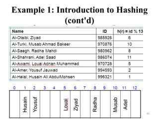
Example 1: Illustrating Hashing
• Use the function f(r) = r.id % 13 to load the following
records into an array of size 13.
985926 1.73 Al-Otaibi, Ziyad
970876 1.60 Al-Turki, Musab Ahmad Bakeer
980962 1.58 Al-Saegh, Radha Mahdi
986074 1.80 Al-Shahrani, Adel Saad
970728 1.73 Al-Awami, Louai Adnan Muhammad
994593 1.66 Al-Amer, Yousuf Jauwad
996321 1.70 Al-Helal, Husain Ali AbdulMohsen
64

65
Example 1: Introduction to Hashing
(cont'd)

Types of Hashing
• There are two types of hashing :
1. Static hashing: In static hashing, the hash function maps
search-key values to a fixed set of locations.
2. Dynamic hashing: In dynamic hashing a hash table can grow
to handle more items. The associated hash function must change
as the table grows.
66

Hash Functions
• A hash function, h, is a function which transforms a key from a set, K,
into an index in a table of size n:
h: K -> {0, 1, ..., n-2, n-1}
• A key can be a number, a string, a record etc. If the keys are strings, hash
function needs more care.
– First convert it into a numeric value.
• A good hash function should:
· Minimize collisions.
· Be easy and quick to compute.
· Distribute key values evenly in the hash table.
· Use all the information provided in the key.
67

Common Hashing Functions
1. Division Remainder (using the table size as
the divisor)
2. Folding
3. Mid-Square
4. Multiplication Method
5. Truncation method
68

Division Remainder (using the table size
as the divisor)
• Computes hash value from key using the % operator.
• Table size that is a power of 2 like 32 and 1024 should be avoided,
for it leads to more collisions. Also, powers of 10 are not good for
table sizes when the keys rely on decimal integers.
• Prime numbers not close to powers of 2 are better table size values.
The hash function is written as,
h(x)=x mod k
The element x to be mapped into one of the array location h of hash
table of size k.
Example: hash table size=12, the key =89 would be mapped to
location
H(89)=89 mod 12=5
69

Folding
• It involves splitting keys into two or more parts and then
combining the parts to form the hash addresses.
• To map the key 25936715 to a range between 0 and 9999, we
can:
· split the number into two as 2593 and 6715 and
· add these two to obtain 9308 as the hash value.
• Very useful if we have keys that are very large.
• Fast and simple especially with bit patterns.
70

Mid-Square
• The key is squared and the middle part of the result taken as the
hash value.
Example: To map the key 3121 into a hash table of size 1000, we
square it 31212 = 9740641 and extract 406 as the hash value.
• Works well if the keys do not contain a lot of leading or trailing
zeros.
71

Multiplication Method
• A very simple variation method on the middle-square method.
• Instead of multiplying the key x by itself, we multiple the key by
a constant A, and then extract the middle k bits from the result.
Example: To map the key 3121 into a hash table of size 1000.
3121*5=15605 middle of this is 560
72

Truncation method
• Works based on the distribution of digits or characters in the
key.
• More evenly distributed digit positions are extracted and used
for hashing purposes.
e.g. 123456789 map to a table of 1000 addresses by picking 3
digits of the key.
73

74
Collision Resolution
• If, when an element is inserted, it hashes to the same value as
an already inserted element, then we have a collision and need
to resolve it.
• There are several methods for dealing with this:
– Open hashing (also known as Separate chaining or
closed addressing)
– Closed hashing (also known as Open addressing)

75
Open hashing
• The idea is to keep a list of all elements that hash to the same
value.
– The array elements are pointers to the first nodes of the
lists.
– A new item is inserted to the front of the list.
• Advantages:
– Better space utilization for large items.
– Simple collision handling: searching linked list.
– Overflow: we can store more items than the hash table size.
– Deletion is quick and easy: deletion from the linked list.

76
Example
0
1
2
3
4
5
6
7
8
9
0
81 1
64 4
25
36 16
49 9
Keys: 0, 1, 4, 9, 16, 25, 36, 49, 64, 81
hash(key) = key % 10.

77
Operations
• Initialization: all entries are set to NULL
• Find:
– locate the cell using hash function.
– sequential search on the linked list in that cell.
• Insertion:
– Locate the cell using hash function.
– (If the item does not exist) insert it as the first item in
the list.
• Deletion:
– Locate the cell using hash function.
– Delete the item from the linked list.

Disadvantage
• Open hashing has the disadvantage of using linked lists.
– Requires the implementation of a second data structure.
78

79
Closed hashing
• In an closed hashing system, all the data go inside the table.
– Thus, a bigger table is needed.
• Generally the load factor should be below 0.5.
– If a collision occurs, alternative cells are tried until an
empty cell is found.
• There are three common collision resolution strategies:
– Linear Probing
– Quadratic probing
– Double hashing

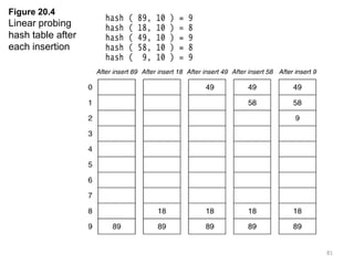
Linear Probing
• The simplest strategy is called linear probing. Suppose that, we
want to store an item in the table.
• Let h  be the hash value for the item, and location h in the
hash table is already occupied.
• With linear probing, the next possible location of storing the
element would be h+1, h+2 and so on. If no such location is
empty, then we look back to the beginning of the table. When
we find an empty location, we store the element there.
80

81
Figure 20.4
Linear probing
hash table after
each insertion

82
Clustering Problem
• As long as table is big enough, a free cell can
always be found, but the time to do so can get
quite large.
• Worse, even if the table is relatively empty,
blocks of occupied cells start forming.
• This effect is known as primary clustering.
• Any key that hashes into the cluster will
require several attempts to resolve the
collision, and then it will add to the cluster.

83
Quadratic Probing
• Quadratic Probing eliminates primary clustering problem
of linear probing.
• Collision function is quadratic.
– The popular choice is f(i) = i2.
• If the hash function evaluates to h and a search in cell h is
inconclusive, we try cells h + 12, h+22, … h + i2.
– i.e. It examines cells 1,4,9 and so on away from the
original probe.
• Remember that subsequent probe points are a quadratic
number of positions from the original probe point.

84
Figure 20.6
A quadratic
probing hash table
after each
insertion (note that
the table size was
poorly chosen
because it is not a
prime number).

85
Quadratic Probing
• Problem:
– We may not be sure that we will probe all locations in the
table (i.e. there is no guarantee to find an empty cell if
table is more than half full.)
– If the hash table size is not prime this problem will be
much severe.
• Although using quadratic probing gives much better
results than linear probing, the problem of cluster
buildup is not avoided altogether. Such clusters are
called secondary clusters.

Double Hashing
• Double hashing is one of the best methods for
dealing with collisions.
– If the slot is full, then a second hash function is
calculated and combined with the first hash
function.
86

87
Double Hashing
• It uses a hash function of the form
– h(x,i) =(h 1 (x)+ i * h2(x))mod k
– Where h 1 and h 2 are hash functions and k is size of TABLE

Consider two auxiliary hash functions are h1(k)=k mod 11
and h2(k)=k mod 9.
insert the keys 76,26,37,59,21,65
Solution:
h 1 (x)=k mod 11
h 2 (x)=k mod 9
Insert 76
h 1 (x)=k mod 11=76 mod 11=10
h 2 (x)=k mod 9=76 mod 9=4
Let i =0
H(76,0)=(10+0*4)mod 11
= 10
88

89
What is the performance problem for static
hashing?
• Long overflow chains can develop and degrade
performance.
– Why poor performance? Scan through overflow chains
linearly.
• How to fix this problem?
– Extendible Hashing: Dynamic techniques to fix this
problem.

90
Extendible Hashing
• Simple Solution – remove overflow chain.
• When bucket (primary page) becomes full, ..
– Re-organize file by adding (doubling) buckets.
• What is the cost concern in doubling buckets?
– High cost: rehash all entries - reading and writing all pages is expensive!
h(key) mod N
h
key
Primary bucket pages
Overflow pages
3*, 5*
97*
0
1
2
.
.
.
N-1
4*, 6*
0*
N
N+1
…
2N-1

91
How to minimize the rehashing cost?
• Use another level of
indirection
– Directory of pointers
to buckets
• Insert 0 (00)
– Double buckets only
double the directory
(no rehashing)
– Split just the bucket
that overflowed!
• What is cost here?
00
01
10
11
Directory
Bucket A
Bucket B
Bucket C
Bucket D
10*
4* 12* 32* 8*
1* 5* 21* 13*
15* 7* 19*
Doubled Directory
Bucket A1
Doubled Directory
Bucket A1

92
Extendible Hashing
• Directory much smaller than file, so doubling much
cheaper. Only one page of data entries is split.
• How to adjust the hash function?
– Before doubling directory
• h(r) → 0..N-1 buckets.
– After doubling directory?
• h(r) → 0 .. 2N-1 (the range is doubled)

Some Applications of Hash Tables
• Database systems: Specifically, those that require efficient random access. Generally,
database systems try to optimize between two types of access methods: sequential and
random. Hash tables are an important part of efficient random access because they provide
a way to locate data in a constant amount of time.
• Symbol tables: The tables used by compilers to maintain information about symbols from
a program. Compilers access information about symbols frequently. Therefore, it is
important that symbol tables be implemented very efficiently.
• Data dictionaries: Data structures that support adding, deleting, and searching for data.
Although the operations of a hash table and a data dictionary are similar, other data
structures may be used to implement data dictionaries. Using a hash table is particularly
efficient.
• Network processing algorithms: Hash tables are fundamental components of several
network processing algorithms and applications, including route lookup, packet
classification, and network monitoring.
• Browser Cashes: Hash tables are used to implement browser cashes.
93

Problems for Which Hash Tables are not Suitable
1. Problems for which data ordering is required.
Because a hash table is an unordered data structure, certain operations are difficult and
expensive. Range queries, proximity queries, selection, and sorted traversals are possible
only if the keys are copied into a sorted data structure. There are hash table implementations
that keep the keys in order, but they are far from efficient.
2. Problems having multidimensional data.
3. Prefix searching especially if the keys are long and of variable-lengths.
4. Problems that have dynamic data:
Open-addressed hash tables are based on 1D-arrays, which are difficult to resize
once they have been allocated. Unless you want to implement the table as a
dynamic array and rehash all of the keys whenever the size changes. This is an
incredibly expensive operation. An alternative is use a separate-chained hash tables or
dynamic hashing.
5. Problems in which the data does not have unique keys.
Open-addressed hash tables cannot be used if the data does not have unique keys. An
alternative is use separate-chained hash tables.
94

Data Structure and algorithms for software

Recommended

More Related Content

Similar to Data Structure and algorithms for software (20)

Recently uploaded (20)

Data Structure and algorithms for software