Data structure using c++
5 likes965 views

This document outlines the syllabus for Computer Science (41) taught by Prof. K. Adisesha. It covers 4 units: Unit A discusses computer hardware components and data structures; Unit B covers object-oriented programming in C++; Unit C focuses on databases, queries, and large data; Unit D examines advanced communication technology concepts like networking and web design. Key topics include motherboards, Boolean algebra, arrays, stacks, queues, classes, inheritance, pointers, files, SQL, networks, and HTML.


![Arrays
26
Data structures
Declaration of array is as follows:
Syntax: Datatype Array_Name [Size];
Example: int arr[10]
Where int specifies the data type or type of
elements arrays stores.
“arr” is the name of array & the number specified
inside the square brackets is the number of
elements an array can store, this is also called sized
or length of array.](https://image.slidesharecdn.com/datastructureusingc-200817174230/85/Data-structure-using-c-26-320.jpg)
![Represent a Linear Array in memory
27
Data structures
The elements of linear array are stored in
consecutive memory locations.
It is shown below:
int A[5]={10, 100, 20, 500, 600}](https://image.slidesharecdn.com/datastructureusingc-200817174230/85/Data-structure-using-c-27-320.jpg)
![Calculating the length of the array
28
Data structures
The elements of array will always be stored in the consecutive
(continues) memory location.
The number of elements that can be stored in an array, that is
the size of array or its length is given by the following
equation:
A[n] is the array size or length of n elements.
The length of the array can be calculated by:
L = UB – LB + 1
To Calculate the address of any element in array:
Loc(A[P])=Base(A)+W(P-LB)
Here, UB is the largest Index and LB is the smallest index
Example: If an array A has values 10, 20, 30, 40, 50, stored in location
0,1, 2, 3, 4 the UB = 4 and LB=0
Size of the array L = 4 – 0 + 1 = 5](https://image.slidesharecdn.com/datastructureusingc-200817174230/85/Data-structure-using-c-28-320.jpg)
![Types of Arrays
29
Data structures
Single Dimension Array
Array with one subscript
Ex: int A[i];
Two Dimension Array
Array with two subscripts (Rows and Column)
Ex: int A[i][j];
Multi Dimension Array
Array with Multiple subscripts
Ex: int A[i][j]..[n];](https://image.slidesharecdn.com/datastructureusingc-200817174230/85/Data-structure-using-c-29-320.jpg)

![Traversing Arrays
31
Data structures
Traversing: It is used to access each data item exactly once so that it
can be processed.
We have linear array A as below:
1 2 3 4 5
10 20 30 40 50
Here we will start from beginning and will go till last element and during this
process we will access value of each element exactly once as below:
A [1] = 10
A [2] = 20
A [3] = 30
A [4] = 40
A [5] = 50](https://image.slidesharecdn.com/datastructureusingc-200817174230/85/Data-structure-using-c-31-320.jpg)


![Insertion Sorting
51
Data structures
ALGORITHM: Insertion Sort (A, N) A is an array with N unsorted
elements.
Step 1: for I=1 to N-1
Step 2: J = I
While(J >= 1)
if ( A[J] < A[J-1] ) then
Temp = A[J];
A[J] = A[J-1];
A[J-1] = Temp;
[End if]
J = J-1
[End of While loop]
[End of For loop]
Step 3: Exit](https://image.slidesharecdn.com/datastructureusingc-200817174230/85/Data-structure-using-c-51-320.jpg)


![Two dimensional array
55
Data structures
A two dimensional array is a collection of elements and each element is
identified by a pair of subscripts. ( A[3] [3] )
The elements are stored in continuous memory locations.
The elements of two-dimensional array as rows and columns.
The number of rows and columns in a matrix is called as the
order of the matrix and denoted as MxN.
The number of elements can be obtained by multiplying number
of rows and number of columns.
A[0] A[1] A[2]
A[0] 10 20 30
A[1] 40 50 60
A[2] 70 80 90](https://image.slidesharecdn.com/datastructureusingc-200817174230/85/Data-structure-using-c-55-320.jpg)
![Representation of Two Dimensional Array
56
Data structures
A two dimensional array is a collection of elements
and each element is identified by a pair of subscripts.
( A[m] [n] )
A is the array of order m x n. To store m*n number of
elements, we need m*n memory locations.
The elements should be in contiguous memory locations.
There are two methods:
o Row-major method
o Column-major method](https://image.slidesharecdn.com/datastructureusingc-200817174230/85/Data-structure-using-c-56-320.jpg)
![Representation of Two Dimensional Array
57
Data structures
Row-Major Method: All the first-row elements are stored in
sequential memory locations and then all the second-row
elements are stored and so on. Ex: A[Row][Col]
Column-Major Method: All the first column elements are
stored in sequential memory locations and then all the second-
column elements are stored and so on. Ex: A [Col][Row]
1000 10 A[0][0]
1002 20 A[0][1]
1004 30 A[0][2]
1006 40 A[1][0]
1008 50 A[1][1]
1010 60 A[1][2]
1012 70 A[2][0]
1014 80 A[2][1]
1016 90 A[2][2]
Row-Major Method
1000 10 A[0][0]
1002 40 A[1][0]
1004 70 A[2][0]
1006 20 A[0][1]
1008 50 A[1][1]
1010 80 A[2][1]
1012 30 A[0][2]
1014 60 A[1][2]
1016 90 A[2][2]
Col-Major Method](https://image.slidesharecdn.com/datastructureusingc-200817174230/85/Data-structure-using-c-57-320.jpg)
![Calculating the length of the 2d-Array
58
Data structures
The elements of array will always be stored in the consecutive
(continues) memory location.
The size of array or its length is given by the following
equation:
A[i][j] is the array size or length of m*n elements.
To Calculate the address of i*j th element in array:
Row-Major Method:
Loc(A[i][j])=Base(A)+W[n(i-LB)+(j-LB)]
Col-Major Method:
Loc(A[i][j])=Base(A)+W[(i-LB)+m(j-LB)]
Here, W is the number of words per memory location and LB is the
smallest index](https://image.slidesharecdn.com/datastructureusingc-200817174230/85/Data-structure-using-c-58-320.jpg)


![PUSH Operation
66
Data structures
The new element is added at the topmost position of the stack.
ALGORITHM:
PUSH (STACK, TOP, SIZE, ITEM)
STACK is the array with N elements. TOP is the pointer to the top of the
element of the array. ITEM to be inserted.
Step 1: if TOP = N then [Check Overflow]
PRINT “ STACK is Full or Overflow”
Exit
[End if]
Step 2: TOP = TOP + 1 [Increment the TOP]
Step 3: STACK[TOP] = ITEM [Insert the ITEM]
Step 4: Return](https://image.slidesharecdn.com/datastructureusingc-200817174230/85/Data-structure-using-c-66-320.jpg)

![POP Operation
68
Data structures
The process of deleting one element or item from the stack is
represented by an operation called as the POP operation.
ALGORITHM: POP (STACK, TOP, ITEM)
STACK is the array with N elements. TOP is the pointer to the top of the
element of the array. ITEM to be DELETED..
Step 1: if TOP = 0 then [Check Underflow]
PRINT “ STACK is Empty or Underflow”
Exit
[End if]
Step 2: ITEM = STACK[TOP] [copy the TOP Element]
Step 3: TOP = TOP - 1 [Decrement the TOP]
Step 4: Return](https://image.slidesharecdn.com/datastructureusingc-200817174230/85/Data-structure-using-c-68-320.jpg)
![PEEK Operation
69
Data structures
The process of returning the top item from the stack
but does not remove it called as the PEEK operation.
ALGORITHM: PEEK (STACK, TOP)
STACK is the array with N elements. TOP is the pointer to the
top of the element of the array.
Step 1: if TOP = NULL then [Check Underflow]
PRINT “ STACK is Empty or Underflow”
Exit
[End if]
Step 2: Return (STACK[TOP] [Return the top
element of the stack]
Step 3:Exit](https://image.slidesharecdn.com/datastructureusingc-200817174230/85/Data-structure-using-c-69-320.jpg)

![Arithmetic Expression
71
Data structures
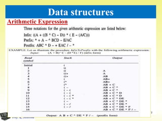
An expression is a combination of operands and operators that
after evaluation results in a single value.
Operand consists of constants and variables.
Operators consists of {, +, -, *, /, ), ] etc.
Expression can be
Infix Expression: If an operator is in between two operands, it is called infix
expression.
Example: a + b, where a and b are operands and + is an operator.
Postfix Expression: If an operator follows the two operands, it is called
postfix expression.
Example: ab +
Prefix Expression: an operator precedes the two operands, it is called prefix
expression.
Example: +ab](https://image.slidesharecdn.com/datastructureusingc-200817174230/85/Data-structure-using-c-71-320.jpg)


![Queue Insertion Operation (ENQUEUE)
82
Data structures
ALGORITHM: ENQUEUE (QUEUE, REAR, FRONT, ITEM)
QUEUE is the array with N elements. FRONT is the pointer that contains the
location of the element to be deleted and REAR contains the location of the
inserted element. ITEM is the element to be inserted.
Step 1: if REAR = N-1 then [Check Overflow] Front Rear
PRINT “QUEUE is Full or Overflow”
Exit
[End if]
Step 2: if FRONT = NULL then [Check Whether Queue is empty]
FRONT = -1
REAR = -1
else
REAR = REAR + 1 [Increment REAR Pointer]
Step 3: QUEUE[REAR] = ITEM [Copy ITEM to REAR position]
Step 4: Return](https://image.slidesharecdn.com/datastructureusingc-200817174230/85/Data-structure-using-c-82-320.jpg)
![Queue Deletion Operation (DEQUEUE)
83
Data structures
ALGORITHM: DEQUEUE (QUEUE, REAR, FRONT, ITEM)
QUEUE is the array with N elements. FRONT is the pointer that contains the
location of the element to be deleted and REAR contains the location of the inserted
element. ITEM is the element to be inserted.
Step 1: if FRONT = NULL then [Check Whether Queue is empty]
PRINT “QUEUE is Empty or Underflow”
Exit
[End if]
Step 2: ITEM = QUEUE[FRONT]
Step 3: if FRONT = REAR then [if QUEUE has only one element]
FRONT = NULL
REAR = NULL
else
FRONT = FRONT + 1 [Increment FRONT pointer]
Step 4: Return](https://image.slidesharecdn.com/datastructureusingc-200817174230/85/Data-structure-using-c-83-320.jpg)


![Operator new and delete
93
Data structures
Operators new allocate memory space.
Operators new [ ] allocates memory space for
array.
Operators delete deallocate memory space.
Operators delete [ ] deallocate memory space for
array.](https://image.slidesharecdn.com/datastructureusingc-200817174230/85/Data-structure-using-c-93-320.jpg)
![Traversing a linked list
94
Data structures
Traversing is the process of accessing each node of the linked
list exactly once to perform some operation.
ALGORITHM: TRAVERS (START, P) START contains
the address of the first node. Another pointer p is temporarily
used to visit all the nodes from the beginning to the end of the
linked list.
Step 1: P = START
Step 2: while P != NULL
Step 3: PROCESS data (P) [Fetch the data]
Step 4: P = link(P) [Advance P to next node]
Step 5: End of while
Step 6: Return](https://image.slidesharecdn.com/datastructureusingc-200817174230/85/Data-structure-using-c-94-320.jpg)


![Inserting node at End
99
Data structures
ALGORITHM: INS_END (START, P)
START contains the address of the first node.
Step 1: START
Step 2: P START [identify the last node]
while P!= null
P next (P)
End while
Step 3: N new Node;
Step 4: data(N) item;
Step 5: link(N) null
Step 6: link(P) N
Step 7: Return](https://image.slidesharecdn.com/datastructureusingc-200817174230/85/Data-structure-using-c-99-320.jpg)
![Inserting node at a given Position
100
Data structures
ALGORITHM: INS_POS (START, P1, P2)
START contains the address of the first node. P2 is new node
Step 1: START
Step 2: P1 START [Initialize node]
Count 0
Step 3: while P!= null
count count+1
P1 next (P1)
End while
Step 4: if (POS=1)
Call function INS_BEG( )
else if (POS=Count +1)
Call function INS_END( )
else if (POS<=Count)
P1 Start
For(i=1; i<=pos; i++)
P1 next(P1);
end for
[create] P2 new node
data(P2) item;
link(P2) link(P1)
link(P1) P2
else
PRINT “Invalid position”
Step 5: Return](https://image.slidesharecdn.com/datastructureusingc-200817174230/85/Data-structure-using-c-100-320.jpg)


![Graph
110
Data structures
Example of graph:
v2
v1
v
4
v5
v3
10
15
8
6
11
9
v4
v1
v2
v4
v3
[a] Directed &
Weighted Graph
[b] Undirected Graph](https://image.slidesharecdn.com/datastructureusingc-200817174230/85/Data-structure-using-c-110-320.jpg)


Data structure using c++
- 1. SECOND PUC Prof. K. Adisesha COMPUTER SCIENCE (41) SYLLABUS
- 2. Learning Outcomes UNIT A 31 Marks Backdrop of Computers 35 hrs UNIT B 39 Marks Computing in C++ 45hrs UNIT C 18 Marks Large Data, Database and Queries 20hrs UNIT D 17 Marks Advanced Concepts in Communication Technology 20hrs 2
- 3. UNIT A Typical configuration of Computer system Review of Block diagram of CPU 4 Marks Mother board Types of Motherboards Components of Motherboard Processor and clock speed BIOS, CMOS Memory and Expansion slots Disk Controllers I/O Ports and Interfaces, BUS Power supply SMPS and UPS 3
- 4. UNIT A BOOLEAN ALGEBRA 13 Marks Development of Boolean Algebra (History) Logical operators Logic gates Basic gates Derived Gates Design of gates NAND to NAND design NOR to NOR design Basic postulates of Boolean Algebra Minimization of Boolean expressions 4
- 5. UNIT A Data structures 14 Marks Introduction to Data Structures Types of Data structures -Linear and non linear Arrays Types of arrays Basic operations Stacks and Queues Data representation Basic operations Applications Linked lists 5
- 6. UNIT B Object Oriented Programming in C++ Review of C++ covered in First PUC 03 Marks Basic concepts of OOPS 04 Marks Classes and objects 06 Marks Declaration & definition of class and objects Access specifies Members of the class Array within class array of objects Functions returning objects 6
- 7. UNIT B Object Oriented Programming in C++ Inheritance(Extending classes) 08 Marks Concepts of Inheritance Visibility modes Levels of inheritance Relationship between classes Pointers 07 Marks Declaration & initialization of pointers Address operator Pointer operator(indirection operator) Pointer arithmetic Pointer and functions 7
- 8. UNIT B Object Oriented Programming in C++ Data file handling 06 Marks Header files(fstream.h) Types of data files Opening & closing files File modes Detecting end of file File pointers Operation on files 8
- 9. UNIT C LARGE DATA, DATABASE AND QUERIES Database Concepts 18 Marks Need for Databases Data Models Keys/ Constraints Relational Algebra Structured Query Language SQL Commands SQL Functions 9
- 10. UNIT D Advanced concepts in communication technology Networking Concepts 09 Marks Evolution of Networking and Protocols Terminologies used in Network Switching techniques Type of Networking Transmission Media Network Topologies Network Devices Network Security 10
- 11. UNIT D Advanced concepts in communication technology Internet and Open source concepts 04 Marks Definition and Applications Internetworking terms and concepts Open source E-commerce Web Designing 04 Marks HTML, -text,layout,images,table,forms,settings XML DYNAMIC HTML Web HOSTING 11
- 12. Data Structures using C++ by Prof. K. Adisesha
- 13. Data structures 14 Marks 13 Introduction to Data Structures Types of Data structures -Linear and non linear Arrays Types of arrays Basic operations Stacks and Queues Data representation Basic operations Applications Linked lists
- 14. Definition 14 Data structures Data: Collection of raw facts. Data structure is representation of the logical relationship existing between individual elements of data. Data structure is a specialized format for organizing and storing data in memory that considers not only the elements stored but also their relationship to each other.
- 15. Definition 15 Data structures Data structure affects the design of both structural & functional aspects of a program. A algorithm is a step by step procedure to solve a particular function. Program=algorithm + Data Structure
- 16. Classification of Data Structure 16 Data structures Data structure are normally divided into two broad categories: Primitive Data Structure Non-Primitive Data Structure
- 17. Classification of Data Structure 17 Data structures
- 18. Primitive Data Structure 18 Data structures There are basic structures and directly operated upon by the machine instructions. Data structures that are directly operated upon the machine-level instructions are known as primitive data structures. Integer, Floating-point number, Character constants, string constants, pointers etc, fall in this category.
- 19. Primitive Data Structure 19 Data structures The most commonly used operation on data structure are broadly categorized into following types: Create Selection Updating Destroy or Delete
- 20. Non-Primitive Data Structure 20 Data structures There are more sophisticated data structures. The Data structures that are derived from the primitive data structures are called Non-primitive data structure. Linear Data structures Non-Linear Data structures The non-primitive data structures emphasize on structuring of a group of homogeneous (same type) or heterogeneous (different type) data items.
- 21. Non-Primitive Data Structure 21 Data structures Linear Data structures: Linear Data structures are kind of data structure that has homogeneous elements. The data structure in which elements are in a sequence and form a liner series. Linear data structures are very easy to implement, since the memory of the computer is also organized in a linear fashion. Some commonly used linear data structures are Stack, Queue and Linked Lists.
- 22. Non-Primitive Data Structure 22 Data structures Non-Linear Data structures: A Non-Linear Data structures is a data structure in which data item is connected to several other data items. Non-Linear data structure may exhibit either a hierarchical relationship or parent child relationship. The data elements are not arranged in a sequential structure. The different non-linear data structures are trees and graphs.
- 23. Non-Primitive Data Structure 23 Data structures The most commonly used operation on data structure are broadly categorized into following types: Traversal Insertion Selection Searching Sorting Merging Destroy or Delete
- 24. Differences between Data Structure 24 Data structures A primitive data structure is generally a basic structure that is usually built into the language, such as an integer, a float. A non-primitive data structure is built out of primitive data structures linked together in meaningful ways, such as a or a linked-list, binary search tree, AVL Tree, graph etc.
- 25. Arrays 25 Data structures An array is defined as a set of finite number of homogeneous elements or same data items. It means an array can contain one type of data only, either all integer, all float-point number or all character.
- 26. Arrays 26 Data structures Declaration of array is as follows: Syntax: Datatype Array_Name [Size]; Example: int arr[10] Where int specifies the data type or type of elements arrays stores. “arr” is the name of array & the number specified inside the square brackets is the number of elements an array can store, this is also called sized or length of array.
- 27. Represent a Linear Array in memory 27 Data structures The elements of linear array are stored in consecutive memory locations. It is shown below: int A[5]={10, 100, 20, 500, 600}
- 28. Calculating the length of the array 28 Data structures The elements of array will always be stored in the consecutive (continues) memory location. The number of elements that can be stored in an array, that is the size of array or its length is given by the following equation: A[n] is the array size or length of n elements. The length of the array can be calculated by: L = UB – LB + 1 To Calculate the address of any element in array: Loc(A[P])=Base(A)+W(P-LB) Here, UB is the largest Index and LB is the smallest index Example: If an array A has values 10, 20, 30, 40, 50, stored in location 0,1, 2, 3, 4 the UB = 4 and LB=0 Size of the array L = 4 – 0 + 1 = 5
- 29. Types of Arrays 29 Data structures Single Dimension Array Array with one subscript Ex: int A[i]; Two Dimension Array Array with two subscripts (Rows and Column) Ex: int A[i][j]; Multi Dimension Array Array with Multiple subscripts Ex: int A[i][j]..[n];
- 30. Basic operations of Arrays 30 Data structures Some common operation performed on array are: Traversing Searching Insertion Deletion Sorting Merging
- 31. Traversing Arrays 31 Data structures Traversing: It is used to access each data item exactly once so that it can be processed. We have linear array A as below: 1 2 3 4 5 10 20 30 40 50 Here we will start from beginning and will go till last element and during this process we will access value of each element exactly once as below: A [1] = 10 A [2] = 20 A [3] = 30 A [4] = 40 A [5] = 50
- 32. Program:To find the frequency of presence element in the given array. 32 Data structures
- 33. Insertion into Array 33 Data structures Insertion: It is used to add a new data item in the given collection of data items. E.g. We have linear array A as below: 1 2 3 4 5 10 20 50 30 15 New element to be inserted is 100 and location for insertion is 3. So shift the elements from 5th location to 3rd location downwards by 1 place. And then insert 100 at 3rd location. It is shown below
- 34. Insertion into Array 34 Data structures It is shown below:
- 35. Insertion into Array: Add a new data item in the given array of data 35 Data structures Program: to add a new data item in the given array of data.
- 36. Deletion from Array 36 Data structures Deletion: It is used to delete an existing data item from the given collection of data items.
- 37. Program to delete an existing data item from the array. 37 Data structures
- 38. Searching in Arrays 38 Data structures Searching: It is used to find out the location of the data item if it exists in the given collection of data items. E.g. We have linear array A as below: 1 2 3 4 5 15 50 35 20 25 Suppose item to be searched is 35. We will start from beginning and will compare 35 with each element. This process will continue until element is found or array is finished. Types of searching Algorithms: Linear searching Binary Searching
- 39. Linear searching 39 Data structures Linear Searching: Also called Sequential Searching. It is used to find out the location of the data item if it exists in the given collection of data items. Example Searching element 33 from the array of elements:
- 40. Linear searching 40 Data structures Linear Searching: Also called Sequential Searching.
- 41. Binary Searching 41 Data structures The binary search algorithm can be used with only sorted list of elements. Binary Search first divides a large array into two smaller sub-arrays and then recursively operate the sub-arrays. Binary Search basically reduces the search space to half at each step
- 42. Binary Searching 42 Data structures The binary search algorithm can be used with only sorted list of elements. Example: Searching the element 5 from the array of elements
- 45. Difference in Searching 45 Data structures
- 46. Difference in Searching 46 Data structures
- 47. Sorting in Arrays 47 Data structures A Sorting Algorithm is used to rearrange a given array or list elements according to a comparison operator on the elements. The comparison operator is used to decide the new order of element in the respective data structure. Types of Sorting Algorithms are: Bubble Sort Insertion Sort Selection Sort Merge Sort Quick Sort Heap Sort Radix Sort Bucket Sort Shell Sort
- 48. Bubble Sort 48 Data structures Bubble Sort is the simplest sorting algorithm that works by repeatedly swapping the adjacent elements if they are in wrong order.
- 49. Insertion Sorting 49 Data structures Insertion sort is a simple sorting algorithm that builds the final sorted array (or list) one item at a time. This is an in-place comparison-based sorting algorithm. Here, a sub-list is maintained which is always sorted.
- 50. Insertion Sorting 50 Data structures This is an in-place comparison-based sorting algorithm. Here, a sub-list is maintained which is always sorted.
- 51. Insertion Sorting 51 Data structures ALGORITHM: Insertion Sort (A, N) A is an array with N unsorted elements. Step 1: for I=1 to N-1 Step 2: J = I While(J >= 1) if ( A[J] < A[J-1] ) then Temp = A[J]; A[J] = A[J-1]; A[J-1] = Temp; [End if] J = J-1 [End of While loop] [End of For loop] Step 3: Exit
- 54. Merging from Array 54 Data structures Merging: It is used to combine the data items of two sorted files into single file in the sorted form We have sorted linear array A as below: 1 2 3 4 5 6 10 40 50 80 95 100 And sorted linear array B as below: 1 2 3 4 20 35 45 90 After merging merged array C is as below: 1 2 3 4 5 6 7 8 9 10 10 20 35 40 45 50 80 90 95 100
- 55. Two dimensional array 55 Data structures A two dimensional array is a collection of elements and each element is identified by a pair of subscripts. ( A[3] [3] ) The elements are stored in continuous memory locations. The elements of two-dimensional array as rows and columns. The number of rows and columns in a matrix is called as the order of the matrix and denoted as MxN. The number of elements can be obtained by multiplying number of rows and number of columns. A[0] A[1] A[2] A[0] 10 20 30 A[1] 40 50 60 A[2] 70 80 90
- 56. Representation of Two Dimensional Array 56 Data structures A two dimensional array is a collection of elements and each element is identified by a pair of subscripts. ( A[m] [n] ) A is the array of order m x n. To store m*n number of elements, we need m*n memory locations. The elements should be in contiguous memory locations. There are two methods: o Row-major method o Column-major method
- 57. Representation of Two Dimensional Array 57 Data structures Row-Major Method: All the first-row elements are stored in sequential memory locations and then all the second-row elements are stored and so on. Ex: A[Row][Col] Column-Major Method: All the first column elements are stored in sequential memory locations and then all the second- column elements are stored and so on. Ex: A [Col][Row] 1000 10 A[0][0] 1002 20 A[0][1] 1004 30 A[0][2] 1006 40 A[1][0] 1008 50 A[1][1] 1010 60 A[1][2] 1012 70 A[2][0] 1014 80 A[2][1] 1016 90 A[2][2] Row-Major Method 1000 10 A[0][0] 1002 40 A[1][0] 1004 70 A[2][0] 1006 20 A[0][1] 1008 50 A[1][1] 1010 80 A[2][1] 1012 30 A[0][2] 1014 60 A[1][2] 1016 90 A[2][2] Col-Major Method
- 58. Calculating the length of the 2d-Array 58 Data structures The elements of array will always be stored in the consecutive (continues) memory location. The size of array or its length is given by the following equation: A[i][j] is the array size or length of m*n elements. To Calculate the address of i*j th element in array: Row-Major Method: Loc(A[i][j])=Base(A)+W[n(i-LB)+(j-LB)] Col-Major Method: Loc(A[i][j])=Base(A)+W[(i-LB)+m(j-LB)] Here, W is the number of words per memory location and LB is the smallest index
- 59. Advantages of Array 59 Data structures It is used to represent multiple data items of same type by using single name. It can be used to implement other data structures like linked lists, stacks, queues, tree, graphs etc. Two-dimensional arrays are used to represent matrices. Many databases include one-dimensional arrays whose elements are records.
- 60. Disadvantages of Array 60 Data structures We must know in advance the how many elements are to be stored in array. Array is static structure. It means that array is of fixed size. The memory which is allocated to array cannot be increased or decreased. Array is fixed size; if we allocate more memory than requirement then the memory space will be wasted. The elements of array are stored in consecutive memory locations. So insertion and deletion are very difficult and time consuming.
- 61. Stack 61 Data structures Stack is a linear data structure which follows a particular order in which the operations are performed. Insertion of element into stack is called PUSH and deletion of element from stack is called POP. The order may be LIFO(Last In First Out) or FILO(First In Last Out).
- 62. Memory Representation of Stack 62 Data structures The stack can be implemented into two ways: Using arrays (Static implementation) Using pointer (Dynamic
- 63. Operation on Stacks 63 Data structures Stack( ): It creates a new stack that is empty. It needs no parameter and returns an empty stack. push(item): It adds a new item to the top of the stack. pop( ): It removes the top item from the stack. peek( ): It returns the top item from the stack but does not remove it. isEmpty( ): It tests whether the stack is empty. size( ): It returns the number of items on the stack.
- 65. PUSH Operation 65 Data structures The process of adding one element or item to the stack is represented by an operation called as the PUSH operation.
- 66. PUSH Operation 66 Data structures The new element is added at the topmost position of the stack. ALGORITHM: PUSH (STACK, TOP, SIZE, ITEM) STACK is the array with N elements. TOP is the pointer to the top of the element of the array. ITEM to be inserted. Step 1: if TOP = N then [Check Overflow] PRINT “ STACK is Full or Overflow” Exit [End if] Step 2: TOP = TOP + 1 [Increment the TOP] Step 3: STACK[TOP] = ITEM [Insert the ITEM] Step 4: Return
- 67. POP Operation 67 Data structures The process of deleting one element or item from the stack is represented by an operation called as the POP operation. When elements are removed continuously from a stack, it shrinks at same end i.e., top
- 68. POP Operation 68 Data structures The process of deleting one element or item from the stack is represented by an operation called as the POP operation. ALGORITHM: POP (STACK, TOP, ITEM) STACK is the array with N elements. TOP is the pointer to the top of the element of the array. ITEM to be DELETED.. Step 1: if TOP = 0 then [Check Underflow] PRINT “ STACK is Empty or Underflow” Exit [End if] Step 2: ITEM = STACK[TOP] [copy the TOP Element] Step 3: TOP = TOP - 1 [Decrement the TOP] Step 4: Return
- 69. PEEK Operation 69 Data structures The process of returning the top item from the stack but does not remove it called as the PEEK operation. ALGORITHM: PEEK (STACK, TOP) STACK is the array with N elements. TOP is the pointer to the top of the element of the array. Step 1: if TOP = NULL then [Check Underflow] PRINT “ STACK is Empty or Underflow” Exit [End if] Step 2: Return (STACK[TOP] [Return the top element of the stack] Step 3:Exit
- 70. Application of Stacks 70 Data structures It is used to reverse a word. You push a given word to stack – letter by letter and then pop letter from the stack. “Undo” mechanism in text editor. Backtracking: This is a process when you need to access the most recent data element in a series of elements. Once you reach a dead end, you must backtrack. Language Processing: Compiler’ syntax check for matching braces in implemented by using stack. Data Conversion of decimal number to binary. To solve tower of Hanoi. Conversion of infix expression into prefix and postfix. Quick sort Runtime memory management.
- 71. Arithmetic Expression 71 Data structures An expression is a combination of operands and operators that after evaluation results in a single value. Operand consists of constants and variables. Operators consists of {, +, -, *, /, ), ] etc. Expression can be Infix Expression: If an operator is in between two operands, it is called infix expression. Example: a + b, where a and b are operands and + is an operator. Postfix Expression: If an operator follows the two operands, it is called postfix expression. Example: ab + Prefix Expression: an operator precedes the two operands, it is called prefix expression. Example: +ab
- 73. Queue 73 Data structures A queue is an ordered collection of items where an item is inserted at one end called the “rear” and an existing item is removed at the other end, called the “front”. Queue is also called as FIFO list i.e. First-In First-Out. In the queue only two operations are allowed enqueue and dequeue. Enqueue means to insert an item into back of the queue. Dequeue means removing the front item.The people standing in a railway reservation row are an example of queue.
- 74. Memory Representation of Queue 74 Data structures The queue can be implemented into two ways: Using arrays (Static implementation) Using pointer (Dynamic
- 75. Memory Representation of a queue using array 75 Data structures Queue is represented in memory using linear array. Let QUEUE is a array, two pointer variables called FRONT and REAR are maintained. The pointer variable FRONT contains the location of the element to be removed or deleted. The pointer variable REAR contains location of the last element inserted. The condition FRONT = NULL indicates that queue is empty. The condition REAR = N-1 indicates that queue is full.
- 76. Types of Queues 76 Data structures Queue can be of four types: o Simple Queue o Circular Queue o Priority Queue o De-queue ( Double Ended Queue)
- 77. Simple Queue 77 Data structures Simple Queue: In simple queue insertion occurs at the rear end of the list and deletion occurs at the front end of the list.
- 78. Circular Queue 78 Data structures Circular Queue: A circular queue is a queue in which all nodes are treated as circular such that the last node follows the first node.
- 79. Priority Queue 79 Data structures A priority queue is a queue that contains items that have some present priority. An element can be inserted or removed from any position depending upon some priority.
- 80. Dequeue Queue 80 Data structures Dequeue: It is a queue in which insertion and deletion takes place at the both ends.
- 81. Operation on Queues 81 Data structures Queue( ): It creates a new queue that is empty. enqueue(item): It adds a new item to the rear of the queue. dequeue( ): It removes the front item from the queue. isEmpty( ): It tests to see whether the queue is empty. size( ): It returns the number of items in the queue.
- 82. Queue Insertion Operation (ENQUEUE) 82 Data structures ALGORITHM: ENQUEUE (QUEUE, REAR, FRONT, ITEM) QUEUE is the array with N elements. FRONT is the pointer that contains the location of the element to be deleted and REAR contains the location of the inserted element. ITEM is the element to be inserted. Step 1: if REAR = N-1 then [Check Overflow] Front Rear PRINT “QUEUE is Full or Overflow” Exit [End if] Step 2: if FRONT = NULL then [Check Whether Queue is empty] FRONT = -1 REAR = -1 else REAR = REAR + 1 [Increment REAR Pointer] Step 3: QUEUE[REAR] = ITEM [Copy ITEM to REAR position] Step 4: Return
- 83. Queue Deletion Operation (DEQUEUE) 83 Data structures ALGORITHM: DEQUEUE (QUEUE, REAR, FRONT, ITEM) QUEUE is the array with N elements. FRONT is the pointer that contains the location of the element to be deleted and REAR contains the location of the inserted element. ITEM is the element to be inserted. Step 1: if FRONT = NULL then [Check Whether Queue is empty] PRINT “QUEUE is Empty or Underflow” Exit [End if] Step 2: ITEM = QUEUE[FRONT] Step 3: if FRONT = REAR then [if QUEUE has only one element] FRONT = NULL REAR = NULL else FRONT = FRONT + 1 [Increment FRONT pointer] Step 4: Return
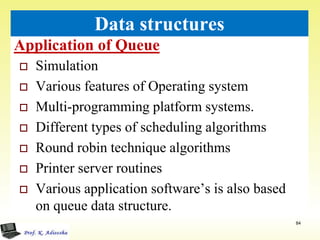
- 84. Application of Queue 84 Data structures Simulation Various features of Operating system Multi-programming platform systems. Different types of scheduling algorithms Round robin technique algorithms Printer server routines Various application software’s is also based on queue data structure.
- 85. Lists 85 Data structures A lists (Linear linked list) can be defined as a collection of variable number of data items called nodes. Lists are the most commonly used non-primitive data structures. Each nodes is divided into two parts: The first part contains the information of the element. The second part contains the memory address of the next node in the list. Also called Link part.
- 86. Types of linked lists 86 Data structures Single linked list Doubly linked list Single circular linked list Doubly circular linked list
- 87. Single linked list 87 Data structures A singly linked list contains two fields in each node - an information field and the linked field. The information field contains the data of that node. The link field contains the memory address of the next node. There is only one link field in each node, the linked list is called singly linked list.
- 88. Single circular linked list 88 Data structures The link field of the last node contains the memory address of the first node, such a linked list is called circular linked list. In a circular linked list every node is accessible from a given node.
- 89. Doubly linked list 89 Data structures It is a linked list in which each node is points both to the next node and also to the previous node. In doubly linked list each node contains three parts: FORW : It is a pointer field that contains the address of the next node BACK: It is a pointer field that contains the address of the previous node. INFO: It contains the actual data. In the first node, if BACK contains NULL, it indicated that it is the first node in the list. The node in which FORW contains, NULL indicates that the node is the last node.
- 90. Doubly circular linked list 90 Data structures It is a linked list in which each node is points both to the next node and also to the previous node. In doubly linked list each node contains three parts: FORW : It is a pointer field that contains the address of the next node BACK: It is a pointer field that contains the address of the previous node. INFO: It contains the actual data.
- 91. Operation on Linked List 91 Data structures The operation that are performed on linked lists are: Creating a linked list Traversing a linked list Inserting an item into a linked list. Deleting an item from the linked list. Searching an item in the linked list Merging two or more linked lists.
- 92. Creating a linked list 92 Data structures The nodes of a linked list can be created by the following structure declaration. struct Node { int info; struct Node *link; }*node1, *node2; Here info is the information field and link is the link field. The link field contains a pointer variable that refers the same node structure. Such a reference is called as Self addressing pointer.
- 93. Operator new and delete 93 Data structures Operators new allocate memory space. Operators new [ ] allocates memory space for array. Operators delete deallocate memory space. Operators delete [ ] deallocate memory space for array.
- 94. Traversing a linked list 94 Data structures Traversing is the process of accessing each node of the linked list exactly once to perform some operation. ALGORITHM: TRAVERS (START, P) START contains the address of the first node. Another pointer p is temporarily used to visit all the nodes from the beginning to the end of the linked list. Step 1: P = START Step 2: while P != NULL Step 3: PROCESS data (P) [Fetch the data] Step 4: P = link(P) [Advance P to next node] Step 5: End of while Step 6: Return
- 95. Inserting a node into the linked list 95 Data structures Inserting a node at the beginning of the linked list Inserting a node at the given position. Inserting a node at the end of the linked list.
- 96. Inserting node at Front 96 Data structures Inserting a node at the beginning of the linked list 1. Create a node. 2. Fill data into the data field of the new node. 3. Mark its pointer field as NULL 4. Attach this newly created node to START 5. Make the new node as the START node.
- 97. Inserting node at Front 97 Data structures ALGORITHM: INS_BEG (START, P) START contains the address of the first node. Step 1: P new Node; Step 2: data(P) num; Step 3: link(P) START Step 4: START P Step 5: Return
- 98. Inserting node at End 98 Data structures
- 99. Inserting node at End 99 Data structures ALGORITHM: INS_END (START, P) START contains the address of the first node. Step 1: START Step 2: P START [identify the last node] while P!= null P next (P) End while Step 3: N new Node; Step 4: data(N) item; Step 5: link(N) null Step 6: link(P) N Step 7: Return
- 100. Inserting node at a given Position 100 Data structures ALGORITHM: INS_POS (START, P1, P2) START contains the address of the first node. P2 is new node Step 1: START Step 2: P1 START [Initialize node] Count 0 Step 3: while P!= null count count+1 P1 next (P1) End while Step 4: if (POS=1) Call function INS_BEG( ) else if (POS=Count +1) Call function INS_END( ) else if (POS<=Count) P1 Start For(i=1; i<=pos; i++) P1 next(P1); end for [create] P2 new node data(P2) item; link(P2) link(P1) link(P1) P2 else PRINT “Invalid position” Step 5: Return
- 101. Deleting an node 101 Data structures Deleting an item from the linked list: Deletion of the first node Deletion of the last node Deletion of the node at the give position
- 102. Deletion of the first node 102 Data structures This algorithm first copies data in the first node to a variable and delete the first node of the linked list. ALGORITHM: DEL_BEG(P, START) This used pointers P Step 1: START Step 2: P START; Step 3: PRINT data(P) Step 4: START Link(P) Step 5: Free(P) Step 6: STOP
- 103. Deleting node from end 103 Data structures
- 104. Deleting node from end 104 Data structures ALGORITHM: DEL_END (P1, P2, START) This used two pointers P1 and P2. Pointer P2 is used to traverse the linked list and pointer P1 keeps the location of the previous node of P2. Step 1: START Step 2: P2 START; Step 3: while ( link(P2) ! = NULL) P1 P2 P2 link(P2) While end Step 4: PRINT data(p2) Step 5: link(P1) NULL Free(P2) Step 6: STOP
- 105. Non-Linear Data structures 105 Data structures A Non-Linear Data structures is a data structure in which data item is connected to several other data items. The data items in non-linear data structure represent hierarchical relationship. Each data item is called node. The different non-linear data structures are Trees Graphs.
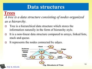
- 106. Trees 106 Data structures A tree is a data structure consisting of nodes organized as a hierarchy. Tree is a hierarchical data structure which stores the information naturally in the form of hierarchy style. It is a non-linear data structure compared to arrays, linked lists, stack and queue. It represents the nodes connected by edges.
- 107. Terminology of a Tree 107 Data structures
- 108. Binary Tree 108 Data structures A binary tree is an ordered tree in which each internal node can have maximum of two child nodes connected to it. A binary tree consists of: A node ( called the root node) Left and right sub trees. A Complete binary tree is a binary tree in which each leaf is at the same distance from the root i.e. all the nodes have maximum two subtrees. Binary tree using array represents a node which is numbered sequentially level by level from left to right. Even empty nodes are numbered.
- 109. Graph 109 Data structures Graph is a mathematical non-linear data structure capable of representing many kind of physical structures. A graph is a set of vertices and edges which connect them. A graph is a collection of nodes called vertices and the connection between them called edges. Definition: A graph G(V,E) is a set of vertices V and a set of edges E.
- 110. Graph 110 Data structures Example of graph: v2 v1 v 4 v5 v3 10 15 8 6 11 9 v4 v1 v2 v4 v3 [a] Directed & Weighted Graph [b] Undirected Graph
- 111. Graph 111 Data structures An edge connects a pair of vertices and many have weight such as length, cost and another measuring instrument for according the graph. Vertices on the graph are shown as point or circles and edges are drawn as arcs or line segment
- 112. Graph 112 Data structures Types of Graphs: Directed graph Undirected graph Simple graph Weighted graph Connected graph Non-connected graph