This document provides an overview of algorithm analysis. It discusses how to analyze the time efficiency of algorithms by counting the number of operations and expressing efficiency using growth functions. Different common growth rates like constant, linear, quadratic, and exponential are introduced. Examples are provided to demonstrate how to determine the growth rate of different algorithms, including recursive algorithms, by deriving their time complexity functions. The key aspects covered are estimating algorithm runtime, comparing growth rates of algorithms, and using Big O notation to classify algorithms by their asymptotic behavior.
Organizing Data in a Traditional File Environment
File organization Term and Concepts
Computer system organizes data in a hierarchy
Bit: Smallest unit of data; binary digit (0,1)
Byte: Group of bits that represents a single character
Field: Group of characters as word(s) or number
Record: Group of related fields
File: Group of records of same type
This document provides an introduction and overview of key topics in software engineering. It discusses what software engineering is, the importance and costs of software development, different types of software projects and applications, and issues like complexity, security and scale that affect software. It also introduces software engineering processes, methods, and ethics. Common questions about the field are addressed. The document is the first chapter of a book on software engineering.
Data Structures and Algorithm - Module 1.pptxEllenGrace9
This document provides an introduction to data structures and algorithms from instructor Ellen Grace Porras. It defines data structures as ways of organizing data to allow for efficient operations. Linear data structures like arrays, stacks, and queues arrange elements sequentially, while non-linear structures like trees and graphs have hierarchical relationships. The document discusses characteristics of good data structures and algorithms, provides examples of common algorithms, and distinguishes between linear and non-linear data structures. It aims to explain the fundamentals of data structures and algorithms.
The document discusses asymptotic notations that are used to describe the time complexity of algorithms. It introduces big O notation, which describes asymptotic upper bounds, big Omega notation for lower bounds, and big Theta notation for tight bounds. Common time complexities are described such as O(1) for constant time, O(log N) for logarithmic time, and O(N^2) for quadratic time. The notations allow analyzing how efficiently algorithms use resources like time and space as the input size increases.
This document provides an overview of trees as a non-linear data structure. It begins by discussing how trees are used to represent hierarchical relationships and defines some key tree terminology like root, parent, child, leaf, and subtree. It then explains that a tree consists of nodes connected in a parent-child relationship, with one root node and nodes that may have any number of children. The document also covers tree traversal methods like preorder, inorder, and postorder traversal. It introduces binary trees and binary search trees, and discusses operations on BSTs like search, insert, and delete. Finally, it provides a brief overview of the Huffman algorithm for data compression.
The document discusses various searching and sorting algorithms. It describes linear search, binary search, and interpolation search for searching unsorted and sorted lists. It also explains different sorting algorithms like bubble sort, selection sort, insertion sort, quicksort, shellsort, heap sort, and merge sort. Linear search searches sequentially while binary search uses divide and conquer. Sorting algorithms like bubble sort, selection sort, and insertion sort are in-place and have quadratic time complexity in the worst case. Quicksort, mergesort, and heapsort generally have better performance.
The document discusses binary trees and their representations and operations. It defines binary trees as trees where each node has at most two child nodes. It also defines complete binary trees as trees where every node has two children except leaf nodes. The document discusses array and linked representations of binary trees and various traversal operations like preorder, inorder and postorder traversals. It also provides code snippets for inserting and deleting nodes from a binary tree.
Binary search is a fast search algorithm that works on sorted data by comparing the middle element of the collection to the target value. It divides the search space in half at each step to quickly locate an element. The algorithm gets the middle element, compares it to the target, and either searches the left or right half recursively depending on if the target is less than or greater than the middle element. An example demonstrates finding the value 23 in a sorted array using this divide and conquer approach.
1. Introduction to time and space complexity.
2. Different types of asymptotic notations and their limit definitions.
3. Growth of functions and types of time complexities.
4. Space and time complexity analysis of various algorithms.
This document provides an introduction to asymptotic analysis of algorithms. It discusses analyzing algorithms based on how their running time increases with the size of the input problem. The key points are:
- Algorithms are compared based on their asymptotic running time as the input size increases, which is more useful than actual running times on a specific computer.
- The main types of analysis are worst-case, best-case, and average-case running times.
- Asymptotic notations like Big-O, Omega, and Theta are used to classify algorithms based on their rate of growth as the input increases.
- Common orders of growth include constant, logarithmic, linear, quadratic, and exponential time.
- A linked list is a data structure where each node contains a data field and a pointer to the next node.
- It allows dynamic size and efficient insertion/deletion compared to arrays.
- A doubly linked list adds a pointer to the previous node, allowing traversal in both directions.
- A circular linked list connects the last node back to the first node, making it a continuous loop.
- Variations require changes to the node structure and functions like append/delete to handle the added previous/next pointers.
1. Asymptotic notation such as Big-O, Omega, and Theta are used to describe the running time of algorithms as the input size n approaches infinity, rather than giving the exact running time.
2. Big-O notation gives an upper bound and describes worst-case running time, Omega notation gives a lower bound and describes best-case running time, and Theta notation gives a tight bound where the worst and best cases are equal up to a constant.
3. Common examples of asymptotic running times include O(1) for constant time, O(log n) for logarithmic time, O(n) for linear time, and O(n^2) for quadratic time.
Binary search trees (BSTs) are data structures that allow for efficient searching, insertion, and deletion. Nodes in a BST are organized so that all left descendants of a node are less than the node's value and all right descendants are greater. This property allows values to be found, inserted, or deleted in O(log n) time on average. Searching involves recursively checking if the target value is less than or greater than the current node's value. Insertion follows the search process and adds the new node in the appropriate place. Deletion handles three cases: removing a leaf, node with one child, or node with two children.
PPT on Analysis Of Algorithms.
The ppt includes Algorithms,notations,analysis,analysis of algorithms,theta notation, big oh notation, omega notation, notation graphs
this is a briefer overview about the Big O Notation. Big O Notaion are useful to check the Effeciency of an algorithm and to check its limitation at higher value. with big o notation some examples are also shown about its cases and some functions in c++ are also described.
The document discusses three sorting algorithms: bubble sort, selection sort, and insertion sort. Bubble sort works by repeatedly swapping adjacent elements that are in the wrong order. Selection sort finds the minimum element and swaps it into the sorted portion of the array. Insertion sort inserts elements into the sorted portion of the array, swapping as needed to put the element in the correct position. Both selection sort and insertion sort have a time complexity of O(n^2) in the worst case.
This document discusses the complexity of algorithms and the tradeoff between algorithm cost and time. It defines algorithm complexity as a function of input size that measures the time and space used by an algorithm. Different complexity classes are described such as polynomial, sub-linear, and exponential time. Examples are given to find the complexity of bubble sort and linear search algorithms. The concept of space-time tradeoffs is introduced, where using more space can reduce computation time. Genetic algorithms are proposed to efficiently solve large-scale construction time-cost tradeoff problems.
Content of slide
Tree
Binary tree Implementation
Binary Search Tree
BST Operations
Traversal
Insertion
Deletion
Types of BST
Complexity in BST
Applications of BST
It is related to Analysis and Design Of Algorithms Subject.Basically it describe basic of topological sorting, it's algorithm and step by step process to solve the example of topological sort.
This document discusses algorithms and their analysis. It begins with definitions of algorithms and their characteristics. Different methods for specifying algorithms are described, including pseudocode. The goal of algorithm analysis is introduced as comparing algorithms based on running time and other factors. Common algorithm analysis methods like worst-case, best-case, and average-case are defined. Big-O notation and time/space complexity are explained. Common algorithm design strategies like divide-and-conquer and randomized algorithms are summarized. Specific algorithms like repeated element detection and primality testing are mentioned.
This document provides an overview of a lecture on designing and analyzing computer algorithms. It discusses key concepts like what an algorithm and program are, common algorithm design techniques like divide-and-conquer and greedy methods, and how to analyze algorithms' time and space complexity. The goals of analyzing algorithms are to understand their behavior, improve efficiency, and determine whether problems can be solved within a reasonable time frame.
This document discusses algorithm analysis and asymptotic notation. It introduces algorithms for computing prefix averages in arrays. One algorithm runs in quadratic time O(n^2) by applying the definition directly. A more efficient linear time O(n) algorithm is also presented that maintains a running sum. Asymptotic analysis determines the worst-case running time of an algorithm as a function of the input size using big-O notation. This provides an analysis of algorithms that is independent of implementation details and hardware.
This document provides an overview of algorithm analysis and asymptotic complexity. It discusses learning outcomes related to analyzing algorithm efficiency using Big O, Omega, and Theta notation. Key points covered include:
- Defining the problem size n and relating algorithm running time to n
- Distinguishing between best-case, worst-case, and average-case complexity
- Using asymptotic notation like Big O to give upper bounds on complexity rather than precise calculations
- Common asymptotic categories like O(n), O(n^2), O(n log n) that classify algorithm growth rates
1. Data structures organize data in memory for efficient access and processing. They represent relationships between data values through placement and linking of the values.
2. Algorithms are finite sets of instructions that take inputs, produce outputs, and terminate after a finite number of unambiguous steps. Common data structures and algorithms are analyzed based on their time and space complexity.
3. Data structures can be linear, with sequential elements, or non-linear, with branching elements. Abstract data types define operations on values independently of implementation through inheritance and polymorphism.
Data Structures and Algorithms Lecture 2: Analysis of Algorithms, Asymptotic ...TechVision8
This document discusses analyzing the running time of algorithms. It introduces pseudocode as a way to describe algorithms, primitive operations that are used to count the number of basic steps an algorithm takes, and asymptotic analysis to determine an algorithm's growth rate as the input size increases. The key points covered are using big-O notation to focus on the dominant term and ignore lower-order terms and constants, and analyzing two algorithms for computing prefix averages to demonstrate asymptotic analysis.
The document discusses the analysis of algorithms, including time and space complexity analysis. It covers key aspects of analyzing algorithms such as determining the basic operation, input size, and analyzing best-case, worst-case, and average-case time complexities. Specific examples are provided, such as analyzing the space needed to store real numbers and analyzing the time complexity of sequential search. Order of growth and asymptotic analysis techniques like Big-O, Big-Omega, and Big-Theta notation are also explained.
This document provides an overview of algorithms including definitions, characteristics, design, and analysis. It defines an algorithm as a finite step-by-step procedure to solve a problem and discusses their key characteristics like input, definiteness, effectiveness, finiteness, and output. The document outlines the design of algorithms using pseudo-code and their analysis in terms of time and space complexity using asymptotic notations like Big O, Big Omega, and Big Theta. Examples are provided to illustrate linear search time complexity and the use of different notations to determine algorithm efficiency.
The document discusses algorithms and data structures. It defines an algorithm as a well-defined procedure that takes input and produces output. Algorithms are used for calculation, data processing, and automated reasoning. The document discusses different ways of describing algorithms including natural language, flowcharts, and pseudo code. It also discusses analyzing the time complexity of algorithms using asymptotic notation such as Big-O, Omega, and Theta notation. Recursive algorithms and solving recurrences are also covered.
The document discusses algorithms, data abstraction, asymptotic analysis, arrays, polynomials, and sparse matrices. It defines algorithms and discusses their advantages and disadvantages. It explains how to design an algorithm and describes iterative and recursive algorithms. It defines data abstraction and gives an example using smartphones. It discusses time and space complexity analysis and different asymptotic notations like Big O, Omega, and Theta. It describes what arrays are, different types of arrays, and applications of arrays. It explains how to represent and add polynomials using linked lists. Finally, it defines sparse matrices and two methods to represent them using arrays and linked lists.
CP4151 Advanced data structures and algorithmsSheba41
The document introduces algorithms and their role in computing. It defines algorithms as tools for solving well-specified computational problems. Algorithms must be correct, producing the appropriate output for each input, and efficient, using as little resources as possible. Examples of algorithms provided include sorting a list alphabetically and determining if a number is prime. Pseudo-code is used to describe algorithms in a language-independent way.
In tube drawing process, a tube is pulled out through a die and a plug to reduce its diameter and thickness as per the requirement. Dimensional accuracy of cold drawn tubes plays a vital role in the further quality of end products and controlling rejection in manufacturing processes of these end products. Springback phenomenon is the elastic strain recovery after removal of forming loads, causes geometrical inaccuracies in drawn tubes. Further, this leads to difficulty in achieving close dimensional tolerances. In the present work springback of EN 8 D tube material is studied for various cold drawing parameters. The process parameters in this work include die semi-angle, land width and drawing speed. The experimentation is done using Taguchi’s L36 orthogonal array, and then optimization is done in data analysis software Minitab 17. The results of ANOVA shows that 15 degrees die semi-angle,5 mm land width and 6 m/min drawing speed yields least springback. Furthermore, optimization algorithms named Particle Swarm Optimization (PSO), Simulated Annealing (SA) and Genetic Algorithm (GA) are applied which shows that 15 degrees die semi-angle, 10 mm land width and 8 m/min drawing speed results in minimal springback with almost 10.5 % improvement. Finally, the results of experimentation are validated with Finite Element Analysis technique using ANSYS.
Lidar for Autonomous Driving, LiDAR Mapping for Driverless Cars.pptxRishavKumar530754
LiDAR-Based System for Autonomous Cars
Autonomous Driving with LiDAR Tech
LiDAR Integration in Self-Driving Cars
Self-Driving Vehicles Using LiDAR
LiDAR Mapping for Driverless Cars
The role of the lexical analyzer
Specification of tokens
Finite state machines
From a regular expressions to an NFA
Convert NFA to DFA
Transforming grammars and regular expressions
Transforming automata to grammars
Language for specifying lexical analyzers
π0.5: a Vision-Language-Action Model with Open-World GeneralizationNABLAS株式会社
今回の資料「Transfusion / π0 / π0.5」は、画像・言語・アクションを統合するロボット基盤モデルについて紹介しています。
拡散×自己回帰を融合したTransformerをベースに、π0.5ではオープンワールドでの推論・計画も可能に。
This presentation introduces robot foundation models that integrate vision, language, and action.
Built on a Transformer combining diffusion and autoregression, π0.5 enables reasoning and planning in open-world settings.
The Fluke 925 is a vane anemometer, a handheld device designed to measure wind speed, air flow (volume), and temperature. It features a separate sensor and display unit, allowing greater flexibility and ease of use in tight or hard-to-reach spaces. The Fluke 925 is particularly suitable for HVAC (heating, ventilation, and air conditioning) maintenance in both residential and commercial buildings, offering a durable and cost-effective solution for routine airflow diagnostics.
We introduce the Gaussian process (GP) modeling module developed within the UQLab software framework. The novel design of the GP-module aims at providing seamless integration of GP modeling into any uncertainty quantification workflow, as well as a standalone surrogate modeling tool. We first briefly present the key mathematical tools on the basis of GP modeling (a.k.a. Kriging), as well as the associated theoretical and computational framework. We then provide an extensive overview of the available features of the software and demonstrate its flexibility and user-friendliness. Finally, we showcase the usage and the performance of the software on several applications borrowed from different fields of engineering. These include a basic surrogate of a well-known analytical benchmark function; a hierarchical Kriging example applied to wind turbine aero-servo-elastic simulations and a more complex geotechnical example that requires a non-stationary, user-defined correlation function. The GP-module, like the rest of the scientific code that is shipped with UQLab, is open source (BSD license).
ADVXAI IN MALWARE ANALYSIS FRAMEWORK: BALANCING EXPLAINABILITY WITH SECURITYijscai
With the increased use of Artificial Intelligence (AI) in malware analysis there is also an increased need to
understand the decisions models make when identifying malicious artifacts. Explainable AI (XAI) becomes
the answer to interpreting the decision-making process that AI malware analysis models use to determine
malicious benign samples to gain trust that in a production environment, the system is able to catch
malware. With any cyber innovation brings a new set of challenges and literature soon came out about XAI
as a new attack vector. Adversarial XAI (AdvXAI) is a relatively new concept but with AI applications in
many sectors, it is crucial to quickly respond to the attack surface that it creates. This paper seeks to
conceptualize a theoretical framework focused on addressing AdvXAI in malware analysis in an effort to
balance explainability with security. Following this framework, designing a machine with an AI malware
detection and analysis model will ensure that it can effectively analyze malware, explain how it came to its
decision, and be built securely to avoid adversarial attacks and manipulations. The framework focuses on
choosing malware datasets to train the model, choosing the AI model, choosing an XAI technique,
implementing AdvXAI defensive measures, and continually evaluating the model. This framework will
significantly contribute to automated malware detection and XAI efforts allowing for secure systems that
are resilient to adversarial attacks.
"Boiler Feed Pump (BFP): Working, Applications, Advantages, and Limitations E...Infopitaara
A Boiler Feed Pump (BFP) is a critical component in thermal power plants. It supplies high-pressure water (feedwater) to the boiler, ensuring continuous steam generation.
⚙️ How a Boiler Feed Pump Works
Water Collection:
Feedwater is collected from the deaerator or feedwater tank.
Pressurization:
The pump increases water pressure using multiple impellers/stages in centrifugal types.
Discharge to Boiler:
Pressurized water is then supplied to the boiler drum or economizer section, depending on design.
🌀 Types of Boiler Feed Pumps
Centrifugal Pumps (most common):
Multistage for higher pressure.
Used in large thermal power stations.
Positive Displacement Pumps (less common):
For smaller or specific applications.
Precise flow control but less efficient for large volumes.
🛠️ Key Operations and Controls
Recirculation Line: Protects the pump from overheating at low flow.
Throttle Valve: Regulates flow based on boiler demand.
Control System: Often automated via DCS/PLC for variable load conditions.
Sealing & Cooling Systems: Prevent leakage and maintain pump health.
⚠️ Common BFP Issues
Cavitation due to low NPSH (Net Positive Suction Head).
Seal or bearing failure.
Overheating from improper flow or recirculation.
2. Objectives
This Chapter introduces students to the analysis
and design of computer algorithms. Upon
completion of this chapter, students will be able to
do the following:
Analyze the asymptotic performance of algorithms.
Demonstrate a familiarity with major algorithms and data
structures.
Apply important algorithmic design paradigms and
methods of analysis.
Synthesize efficient algorithms in common engineering
design situations.
2
4. What is an Algorithm?
Algorithms are the ideas behind computer
programs.
Algorithm is any well-defined computational
procedure that takes some value, or set of
values, as input and produces some value,
or set of values, as output.
Algorithm is thus a sequence of
computational steps that transform the
input into the output. 4
5. What is an Algorithm?
Example:
Directions to somebody’s house is an
algorithm.
A recipe for cooking a cake is an algorithm.
5
6. What is a Program?
A program is a set of instructions which the
computer will follow to solve a problem
6
7. Introduction
Why we need algorithm analysis ?
Writing a working program is not good enough.
The program may be inefficient!
If the program is run on a large data set, then
the running time becomes an issue.
7
8. What to Analyze ?
Correctness
Does the input/output relation match algorithm
requirement?
Amount of work done
Basic operations to do task finite amount of time
Amount of space used
Memory used
8
9. What to Analyze ?
Simplicity, clarity
Verification and implementation.
Optimality
Is it impossible to do better?
9
10. What to Analyze ?
Time Complexity
Amount of computer time it needs to
execute the program to get the intended
result.
Space Complexity
Memory requirements based on the
problem size.
10
11. 11
Properties of algorithms
Input: what the algorithm takes in as input
Output: what the algorithm produces as output
Definiteness: the steps are defined precisely
Correctness: should produce the correct output
Finiteness: the steps required should be finite
Effectiveness: each step must be able to be
performed in a finite amount of time.
12. What is DS & Algorithm ?
Data Structure is a systematic way of
organizing and accessing data.
Algorithm is a step-by-step procedure for
performing some task in a finite amount of
time.
13. Types of DS
Linear data structures:
Array
Linked list
Stack
Queue
Non-linear data structures:
Graphs
Trees
14. Linear & nonlinear Data Structures
Main difference between linear & nonlinear
data structures lie in the way they organize
data elements.
In linear data structures, data elements are
organized sequentially and therefore they
are easy to implement in the computer’s
memory.
In nonlinear data structures, a data element
can be attached to several other data
elements to represent specific relationships
that exist among them. 18
15. Linear & nonlinear Data Structures
Due to this nonlinear structure, they might
be difficult to be implemented in computer’s
linear memory compared to implementing
linear data structures.
Selecting one data structure type over the
other should be done carefully by
considering the relationship among the
data elements that needs to be stored.
19
16. Array
An array is a collection of homogeneous
type of data elements.
An array is consisting of a collection of
elements .
20
17. Stack
A Stack is a list of elements in which an
element may be inserted or deleted at one
end which is known as TOP of the stack.
21
19. STACKS
A stack is a restricted linear list in which all additions
and deletions are made at one end, the top.
If we insert a series of data items into a stack and then
remove them, the order of the data is reversed.
This reversing attribute is why stacks are known as
last in, first out (LIFO) data structures.
Figure:-Three representations of stacks
20. Applications
Data Structures are applied extensively in
Operating System,
Database Management System,
Statistical analysis package,
Numerical Analysis
Graphics,
Artificial Intelligence,
Simulation
22. Asymptotic Notation (O, , )
26
Asymptotic notations are the terminology
that enables meaningful statements about
time & space complexity.
To Calculate Running Time of an algorithm
23. Asymptotic Notation (O, , )
27
The time required by the given algorithm
falls under three types
1. Best-case time or the minimum time required
in executing the program.
2. Average case time or the average time
required in executing program.
3. Worst-case time or the maximum time
required in executing program.
25. Time Complexity ---- For Loop
Statement
for(i=0; i <n; i++)
Total time=time(stmt1)+time(stmt2)+….+time(stmt n)
Note: For declarations, time count is 0
29
n+11 n
Total : 1+n+1+n = 2n+2 O(n)
26. Time Complexity ---- If-Else
Statement
if(condition)
{
stmt 1;
}
else
{
stmt2;
}
30
Either Stmt1 or Stmt2 will execute.
So, Worst case is
Max(time(stmt1, stmt2)
Max (O(n), O(1)) O(n)
27. Nested For loops
for(i=0; i <n; i++)
{
for(i=0; i <n; i++)
{
Stmts;
}
}
Note: For all the “for loop” statement multiplied
by the product.
31
Total : n *n O(n2)
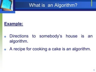
28. Tabular Method
32
Iterative function to sum a list of numbers
Statement Frequency
float sum(float list[ ], int n)
{
float tempsum = 0;
int i;
for(i=0; i <n; i++)
tempsum += list[i];
return tempsum;
}
0
0
1
0
n+1
n
1
0
Total 2n+3
steps/execution
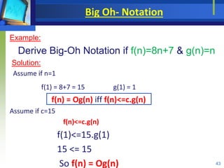
29. 33
Statement s/e Frequency Total steps
float rsum(float list[ ], int n)
{
if (n)
return rsum(list, n-1)+list[n-1];
return list[0];
}
0 0 0
0 0 0
1 n+1 n+1
1 n n
1 1 1
0 0 0
Total 2n+2
Step count table for recursive summing function
30. Examples
Examples of Big Oh (O) Notation
34
O(1) Constant
O(n) Linear
O(n2) Quadratic
O(n3) Cubic
O(2n) Exponential
O(log n) Logarithm
31. 35
Analysis of Algorithms
An algorithm is a finite set of precise instructions
for performing a computation or for solving a
problem.
What is the goal of analysis of algorithms?
To compare algorithms mainly in terms of
running time but also in terms of other factors
(e.g., memory requirements, programmer's
effort etc.)
What do we mean by running time analysis?
Determine how running time increases as the
size of the problem increases.
32. 36
How do we compare algorithms?
We need to define a number of objective
measures.
(1) Compare execution times?
Not good: times are specific to a particular
computer !!
(2) Count the number of statements executed?
Not good: number of statements vary with
the programming language as well as the
style of the individual programmer.
33. 37
Ideal Solution
Express running time as a function of the
input size n (i.e., f(n)).
Compare different functions corresponding
to running times.
Such an analysis is independent of machine
time, programming style, etc.
36. Big Oh- Notation
Denoted by “O”.
Using this we can compute the max possible
amount of time that an algorithm will take for
its application.
Consider f(n) and g(n) to be two positive
function of “n” where the “n” is the input size.
f(n) = Og(n) iff f(n)<=c.g(n)
C>0 ; n0<n
41
38. Big Oh- Notation
Example:
Derive Big-Oh Notation if f(n)=8n+7 & g(n)=n
Solution:
Assume if n=1
f(1) = 8+7 = 15 g(1) = 1
f(n) = Og(n) iff f(n)<=c.g(n)
Assume if c=15
f(n)<=c.g(n)
f(1)<=15.g(1)
15 <= 15
So f(n) = Og(n) 43
39. Big Oh- Notation
Step- II
Assume if n=2
f(2) = 16+7 = 23 g(2) = 2
f(2)<=15.g(2)
23 <= 30
So f(n) = Og(n)
44
40. Big Oh- Notation
Step- III
Assume if n=3
f(3) = 24+7 = 31 g(3) = 3
f(2)<=15.g(2)
31 <= 45
So f(n) = Og(n)
Conclusion: f(n)<=c.g(n); for c=15 & n0 = 1
45
41. Omega Notation
Denoted by “”.
Using this we can compute the minimum
amount of time that an algorithm will take for
its computation.
Consider f(n) and g(n) to be two positive
function of “n” where the “n” is the input size.
f(n) = g(n) iff f(n)>=c.g(n)
C>0 ; n0<n
46
43. Theta Notation
Denoted by “”.
Using this we can compute the average
amount of time that an algorithm will take for
its computation.
f(n) = g(n)
iff c1.g(n) <= f(n) <=c2.g(n)
48
45. University Questions – Ch 1 & 2
Distinguish between datatype and data structure.
Define O notation.
What is recursive function? State its advantages
What are linear and non-linear Data Structures
What are Asymptotic Notation
Why is it necessary to analyze an algorithm
What is Data Structure and Abstract Data Type?
Explain the Asymptotic notation to measure the
time complexity of an algorithm?
50
46. University Questions – Ch 1 & 2
What is Recursion? Give disadvantages of recursion.
Write a program to implement Towers of Hanoi .10 M
Explain Asymptotic Notations and write the properties
of asymptotic notations 10 M
51