
![eventually be constructed. By providing this level of abstraction, we are creating an
encapsulation around the data. The idea is that by encapsulating the details of the
implementation, we are hiding them from the user’s view. This is called information hiding.
The implementation of an abstract data type, often referred to as a data structure, will require
that we provide a physical view of the data using some collection of programming constructs
and primitive data types.
An ADT consists of an abstract data structure and operations. Put in other terms, an ADT is an
abstraction of a data structure. The ADT specifies:
- What can be stored in the Abstract Data Type?
- What operations can be done on/by the Abstract Data Type?
For example, if we are going to model employees of an organization:
This ADT stores employees with their relevant attributes (EmpName, EmpID, Salary, etc) and
discarding irrelevant attributes. This ADT supports hiring, firing, retiring as operations on data.
Therefore, A data structure can be a language construct that the programmer has defined in
order to implement an abstract data type.
1.1.1. Classifications of Data structure
Data structures are broadly divided into two types:
1. Primitive data structures.
2. Non-primitive data structures
1. Primitive Data structures are basic data structure which is directly supported by the
programming language ie; any operation is directly performed in these data items. Ex:
integer, Character, Boolean, float, double, string, pointer etc. These primitive data structure
are the basis for the discussion of more sophisticated (non-primitive) data structures.
2. Non-primitive data structures are not defined by the programming language, but are
instead created by the programmer. Non primitive Data structures are more sophisticated
data structure emphasizing on structuring of a group of homogenous (same type) or
heterogeneous (different type) data items. Eg, Array, stack, queue, list, files, linked list, trees
and graph fall in this category. Non-primitive data structures can also be categorized in to:
1. Linear data structure
2. Nonlinear data structure
1. Linear data structures: These type data structures organize their data elements in a linear
fashion, where data elements are attached one after the other. They are very easy to
implement, since the memory of the computer is also organized in a linear fashion. Some
commonly used linear data structures are arrays, linked lists, stacks and queues.
Arrays: is a collection of similar type of data items and each data item is called an
element of the array. The data type of the element may be any valid data type like char,
int, float or double. The elements of array share the same variable name but each one
carries a different index number known as subscript. The array can be one dimensional,
two dimensional or multidimensional. The individual elements of the array age are:
age[0], age[1], age[2], age[3],......... age[98], age[99].
Linked List: is a linear data structure which is used to maintain a list in the memory. It
can be seen as the collection of nodes stored at non-contiguous memory locations. Each
node of the list contains a pointer to its adjacent node.
2](https://image.slidesharecdn.com/datastructuresandalgorithmcha1and2-250314211850-11dad352/85/data-structures-and-algorithm-Cha-1and-2-doc-2-320.jpg)


![Chapter 2. Simple Sorting and Searching Algorithms
2.1. Searching
Searching is a process of looking for a specific element in a list of items or determining that the
item is not in the list. There are two simple searching algorithms:
• Sequential Search, and
• Binary Search
2.1.1. Linear Search (Sequential Search)
Pseudocode
Loop through the array starting at the first element until the value of target matches one of the
array elements.
If a match is not found, return –1.
Time is proportional to the size of input (n) and
we call this time complexity O(n)
.
Example Implementation:
int Linear_Search(int list[], int key)
{
int index=0;
int found=0;
do{
if(key==list[index])
found=1;
else
index++;
}while(found==0&&index<n);
if(found==0)
index=-1;
return index;
}
2.1.2. Binary Search
This searching algorithm works only on an ordered list:
Pseudocode](https://image.slidesharecdn.com/datastructuresandalgorithmcha1and2-250314211850-11dad352/85/data-structures-and-algorithm-Cha-1and-2-doc-18-320.jpg)
![• Locate midpoint of array to search
• Determine if target is in lower half or upper half of an array.
o If in lower half, make this half the array to search
o If in the upper half, make this half the array to search
• Loop back to step 1 until the size of the array to search is one, and this element does not
match, in which case return –1.
The computational time for this algorithm is proportional to log2 n
. Therefore the time complexity is O(log n)
Example Implementation:
int Binary_Search(int list[],int k)
{
int left=0;
int right=n-1;
int found=0;
do{
mid=(left+right)/2;
if(key==list[mid])
found=1;
else{
if(key<list[mid])
right=mid-1;
else
left=mid+1;
}
}while(found==0&&left<right);
if(found==0)
index=-1;
else
index=mid;
return index;
}
2.2. Sorting Algorithms
Sorting is one of the most important operations performed by computers. Sorting is a process of
reordering a list of items in either increasing or decreasing order. The following are simple
sorting algorithms used to sort small-sized lists.
• Insertion Sort](https://image.slidesharecdn.com/datastructuresandalgorithmcha1and2-250314211850-11dad352/85/data-structures-and-algorithm-Cha-1and-2-doc-19-320.jpg)

![2.2.1. Insertion Sort
The insertion sort works just like its name suggests - it inserts each item into its proper place in
the final list. The simplest implementation of this requires two list structures - the source list and
the list into which sorted items are inserted. To save memory, most implementations use an in-
place sort that works by moving the current item past the already sorted items and repeatedly
swapping it with the preceding item until it is in place.
It's the most instinctive type of sorting algorithm. The approach is the same approach that you
use for sorting a set of cards in your hand. While playing cards, you pick up a card, start at the
beginning of your hand and find the place to insert the new card, insert it and move all the others
up one place.
Basic Idea:
Find the location for an element and move all others up, and insert the element.
The process involved in insertion sort is as follows:
1. The left most value can be said to be sorted relative to itself. Thus, we don’t need to do
anything.
2. Check to see if the second value is smaller than the first one. If it is swap these two values.
The first two values are now relatively sorted.
3. Next, we need to insert the third value in to the relatively sorted portion so that after
insertion, the portion will still be relatively sorted.
4. Remove the third value first. Slide the second value to make room for insertion. Insert the
value in the appropriate position.
5. Now the first three are relatively sorted.
6. Do the same for the remaining items in the list.
Implementation
void insertion_sort(int list[]){
int temp;
for(int i=1;i<n;i++){
temp=list[i];
for(int j=i; j>0 && temp<list[j-1];j--)
{ // work backwards through the array finding where temp should go
list[j]=list[j-1];
list[j-1]=temp;
}//end of inner loop
}//end of outer loop
}//end of insertion_sort
Analysis
The body of insertion_sort is made up of two nested for loops. The outer for](https://image.slidesharecdn.com/datastructuresandalgorithmcha1and2-250314211850-11dad352/85/data-structures-and-algorithm-Cha-1and-2-doc-21-320.jpg)
![loop is executed n - 1 times.i.e:
How many comparisons?
1+2+3+…+(n-1)= O(n2
)
For the inner for loop is the total number of comparisons will be(Counting comparisons
or swaps yields similar results.)
How many swaps?
1+2+3+…+(n-1)= O(n2
)
How much space?
In-place algorithm
2.2.2. Selection Sort
Basic Idea:
Loop through the array from i=0 to n-1.
Select the smallest element in the array from I to n
Swap this value with value at position i.
Implementation:
void selection_sort(int list[])
{
int i,j, smallest;
for(i=0;i<n;i++){
smallest=i;
for(j=i+1;j<n;j++){
if(list[j]<list[smallest])
smallest=j;
}//end of inner loop
temp=list[smallest];
list[smallest]=list[i];
list[i]=temp;
} //end of outer loop
}//end of selection_sort
Analysis
Selection Sort first finds the smallest key in an unsorted list, then the second
smallest, and so on. Its unique feature is that there are few record swaps. To find
the next smallest key value requires searching through the entire unsorted portion
of the array, but only one swap is required to put the record in place. Thus, the total
number of swaps required will be n-1.](https://image.slidesharecdn.com/datastructuresandalgorithmcha1and2-250314211850-11dad352/85/data-structures-and-algorithm-Cha-1and-2-doc-22-320.jpg)
![How many comparisons?
(n-1)+(n-2)+…+1= O(n2
)
How many swaps?
n=O(n)
How much space?
In-place algorithm
2.2.3. Bubble Sort
Bubble Sort consists of a simple double for loop. The first iteration of the
inner for loop moves through the record array from bottom to top, comparing
adjacent keys. If the lower-indexed key’s value is greater than its higher-indexed
neighbor, then the two values are swapped. Once the smallest value is encountered,
this process will cause it to “bubble” up to the top of the array. The second pass
through the array repeats this process.
Bubble sort is the simplest algorithm to implement and the slowest algorithm on very large
inputs.
Basic Idea:
Loop through array from i=0 to n and swap adjacent elements if they are out of order.
Implementation:
void bubble_sort(list[])
{
int i,j;
for(int i=0;i<n; i++){
for(j=n-1;j>i; j--){
if(list[j]<list[j-1]){
temp=list[j];
list[j]=list[j-1];
list[j-1]=temp;
}//swap adjacent elements
}//end of inner loop
}//end of outer loop
}//end of bubble_sort
Analysis of Bubble Sort
How many comparisons?](https://image.slidesharecdn.com/datastructuresandalgorithmcha1and2-250314211850-11dad352/85/data-structures-and-algorithm-Cha-1and-2-doc-23-320.jpg)

![Chapter 3. Data Structures
3.1. Structures
Structures are aggregate data types built using elements of primitive data types.
struct Time{
int hour;
int minute;
int second;
};
The struct keyword creates a new user defined data type that is used to declare variables of an
aggregate data type.
Structure variables are declared like variables of other types.
Syntax: struct <structure tag> <variable name>;
E.g. struct Time timeObject,
struct Time *timeptr;
3.1.1. Accessing Members of Structure Variables
The Dot operator (.): to access data members of structure variables.
The Arrow operator (->): to access data members of pointer variables pointing to the structure.
E.g. Print member hour of timeObject and timeptr.
cout<< timeObject.hour; or
cout<<timeptr->hour;
TIP: timeptr->hour is the same as (*timeptr).hour.
The parentheses is required since (*) has lower precedence than (.).
3.1.2. Self-Referential Structures
Structures can hold pointers to instances of themselves.
struct list{
char name[10];
int count;
struct list *next;
};
However, structures cannot contain instances of themselves.
3.2. Linked Lists
Linked lists are the most basic self-referential structures. Linked lists allow you to have a chain
of structs with related data.](https://image.slidesharecdn.com/datastructuresandalgorithmcha1and2-250314211850-11dad352/85/data-structures-and-algorithm-Cha-1and-2-doc-25-320.jpg)

![This linked list has four nodes in it, each with a link to the next node in the series. The last node
has a link to the special value NULL, which any pointer (whatever its type) can point to, to
show that it is the last link in the chain. There is also another special pointer, called Start (also
called head), which points to the first link in the chain so that we can keep track of it.
3.2.3. Defining the data structure for a linked list
The key part of a linked list is a structure, which holds the data for each node (the name,
address, age or whatever for the items in the list), and, most importantly, a pointer to the next
node. Here we have given the structure of a typical node:
struct node
{ char name[20]; // Name of up to 20 letters
int age
float height; // In metres
node *nxt;// Pointer to next node
};
node *start_ptr = NULL;
The important part of the structure is the line before the closing curly brackets. This gives a
pointer to the next node in the list. This is the only case in C++ where you are allowed to refer
to a data type (in this case node) before you have even finished defining it!
We have also declared a pointer called start_ptr that will permanently point to the start of the
list. To start with, there are no nodes in the list, which is why start_ptr is set to NULL.
3.2.4. Adding a node to the end of the list
The first problem that we face is how to add a node to the list. For simplicity's sake, we will
assume that it has to be added to the end of the list, although it could be added anywhere in the
list (a problem we will deal with later on).
Firstly, we declare the space for a pointer item and assign a temporary pointer to it. This is done
using the new statement as follows:
temp = new node;
We can refer to the new node as *temp, i.e. "the node that temp points to". When the fields of
this structure are referred to, brackets can be put round the *temp part, as otherwise the compiler
will think we are trying to refer to the fields of the pointer. Alternatively, we can use the arrow
pointer notation.](https://image.slidesharecdn.com/datastructuresandalgorithmcha1and2-250314211850-11dad352/85/data-structures-and-algorithm-Cha-1and-2-doc-27-320.jpg)


![Pop()
{
if stack not empty {
return the value of the top item
remove the top item from the stack
} else {
give an error message
}
}
CreateStack()
{
remove existing items from the stack
initialise the stack to empty
}
4.1
Array Implementation of Stacks: The PUSH operation
Here, as you might have noticed, addition of an element is known as the PUSH operation. So, if
an array is given to you, which is supposed to act as a STACK, you know that it has to be a
STATIC Stack; meaning, data will overflow if you cross the upper limit of the array. So, keep
this in mind.
Algorithm:
Step-1: Increment the Stack TOP by 1. Check whether it is always less than the Upper Limit of
the stack. If it is less than the Upper Limit go to step-2 else report -"Stack Overflow"
Step-2: Put the new element at the position pointed by the TOP
Implementation:
static int stack[UPPERLIMIT];
int top= -1; /*stack is empty*/
..
..
main()
{
..
..
push(item);
..
..
}
push(int item)
{](https://image.slidesharecdn.com/datastructuresandalgorithmcha1and2-250314211850-11dad352/85/data-structures-and-algorithm-Cha-1and-2-doc-41-320.jpg)
![top = top + 1;
if(top < UPPERLIMIT)
stack[top] = item; /*step-1 & 2*/
else
cout<<"Stack Overflow";
}
Note:- In array implementation,we have taken TOP = -1 to signify the empty stack, as this
simplifies the implementation.
4.2 Array Implementation of Stacks: the POP operation
POP is the synonym for delete when it comes to Stack. So, if you're taking an array as the stack,
remember that you'll return an error message, "Stack underflow", if an attempt is made to Pop
an item from an empty Stack. OK.
Algorithm
Step-1: If the Stack is empty then give the alert "Stack underflow" and quit; or else go to step-2
Step-2: a) Hold the value for the element pointed by the TOP
b) Put a NULL value instead
c) Decrement the TOP by 1
Implementation:
static int stack[UPPPERLIMIT];
int top=-1;
..
..
main()
{
..
..
poped_val = pop();
..
..
}
int pop()
{
int del_val = 0;
if(top == -1)
cout<<"Stack underflow"; /*step-1*/
else
{](https://image.slidesharecdn.com/datastructuresandalgorithmcha1and2-250314211850-11dad352/85/data-structures-and-algorithm-Cha-1and-2-doc-42-320.jpg)
![del_val = stack[top]; /*step-2*/
stack[top] = NULL;
top = top -1;
}
return(del_val);
}
Note: - Step-2:(b) signifies that the respective element has been deleted.
Algorithm
Step-1: If the Stack is empty go to step-2 or else go to step-3
Step-2: Create the new element and make your "stack" and "top" pointers point to it and quit.
Step-3: Create the new element and make the last (top most) element of the stack to point to it
Step-4: Make that new element your TOP most element by making the "top" pointer point to it.
Implementation:
struct node
{
int item;
struct node *next;
}
struct node *stack = NULL; /*stack is initially empty*/
struct node *top = stack;
main()
{
..
..
push(item);
..
}
push(int item)
{
if(stack == NULL) /*step-1*/
{
newnode = new node /*step-2*/
newnode -> item = item;
newnode -> next = NULL;
stack = newnode;
top = stack;
}
else
{
newnode = new node; /*step-3*/
newnode -> item = item;
newnode -> next = NULL;
top ->next = newnode;
top = newnode; /*step-4*/](https://image.slidesharecdn.com/datastructuresandalgorithmcha1and2-250314211850-11dad352/85/data-structures-and-algorithm-Cha-1and-2-doc-43-320.jpg)
![}
}
4.3 Linked List Implementation of Stacks: the PUSH operation
It’s very similar to the insertion operation in a dynamic singly linked list. The only difference is
that here you'll add the new element only at the end of the list, which means addition can happen
only from the TOP. Since a dynamic list is used for the stack, the Stack is also dynamic, means
it has no prior upper limit set. So, we don't have to check for the Overflow condition at all!
In Step [1] we create the new element to be pushed
to the Stack.
In Step [2] the TOP most element is made to point
to our newly created element.
In Step [3] the TOP is moved and made to point to
the last element in the stack, which is our newly
added element.
4.4 Linked List Implementation of Stacks: the POP Operation
This is again very similar to the deletion operation in any Linked List, but you can only delete
from the end of the list and only one at a time; and that makes it a stack. Here, we'll have a list
pointer, "target", which will be pointing to the last but one element in the List (stack). Every
time we POP, the TOP most element will be deleted and "target" will be made as the TOP most
element.
In step[1] we got the "target" pointing to the last but one node.
In step[2] we freed the TOP most element.
In step[3] we made the "target" node as our TOP most element.
Supposing you have only one element left in the Stack, then we won't
make use of "target" rather we'll take help of our "bottom" pointer. See
how...
Algorithm:
Step-1: If the Stack is empty then give an alert message "Stack Underflow" and quit; or else proceed
Step-2: If there is only one element left go to step-3 or else step-4
Step-3: Free that element and make the "stack", "top" and "bottom" pointers point to NULL and quit
Step-4: Make "target" point to just one element before the TOP; free the TOP most element; make
"target" as your TOP most element
Implementation:
struct node
{
int nodeval;
struct node *next;
}](https://image.slidesharecdn.com/datastructuresandalgorithmcha1and2-250314211850-11dad352/85/data-structures-and-algorithm-Cha-1and-2-doc-44-320.jpg)


![Chapter 5. Queues
a data structure that has access to its data at the front and rear.
operates on FIFO (Fast In First Out) basis.
uses two pointers/indices to keep tack of information/data.
has two basic operations:
o enqueue - inserting data at the rear of the queue
o dequeue – removing data at the front of the queue
Example:
Operation Content of queue
Enqueue(B) B
Enqueue(C) B, C
Dequeue() C
Enqueue(G) C, G
Enqueue (F) C, G, F
Dequeue() G, F
Enqueue(A) G, F, A
Dequeue() F, A
5.1. Simple array implementation of enqueue and dequeue operations
Analysis:
Consider the following structure: int Num[MAX_SIZE];
We need to have two integer variables that tell:
- the index of the front element
- the index of the rear element
We also need an integer variable that tells:
- the total number of data in the queue
int FRONT =-1,REAR =-1;
int QUEUESIZE=0;
To enqueue data to the queue
o check if there is space in the queue
REAR<MAX_SIZE-1 ?
Yes: - Increment REAR
Front Rear
dequeue enqueue](https://image.slidesharecdn.com/datastructuresandalgorithmcha1and2-250314211850-11dad352/85/data-structures-and-algorithm-Cha-1and-2-doc-52-320.jpg)
![- Store the data in Num[REAR]
- Increment QUEUESIZE
FRONT = = -1?
Yes: - Increment FRONT
No: - Queue Overflow
To dequeue data from the queue
o check if there is data in the queue
QUEUESIZE > 0 ?
Yes: - Copy the data in Num[FRONT]
- Increment FRONT
- Decrement QUEUESIZE
No: - Queue Underflow
Implementation:
const int MAX_SIZE=100;
int FRONT =-1, REAR =-1;
int QUEUESIZE = 0;
void enqueue(int x)
{
if(Rear<MAX_SIZE-1)
{
REAR++;
Num[REAR]=x;
QUEUESIZE++;
if(FRONT = = -1)
FRONT++;
}
else
cout<<"Queue Overflow";
}
int dequeue()
{
int x;
if(QUEUESIZE>0)
{
x=Num[FRONT];
FRONT++;
QUEUESIZE--;
}
else
cout<<"Queue Underflow";
53](https://image.slidesharecdn.com/datastructuresandalgorithmcha1and2-250314211850-11dad352/85/data-structures-and-algorithm-Cha-1and-2-doc-53-320.jpg)
![return(x);
}
5.2. Circular array implementation of enqueue and dequeue operations
A problem with simple arrays is we run out of space even if the queue never reaches the size of
the array. Thus, simulated circular arrays (in which freed spaces are re-used to store data) can be
used to solve this problem.
Example: Consider a queue with MAX_SIZE = 4
Operation
Simple array Circular array
Content of
the array
Content of
the Queue
QUEUE
SIZE
Message Content of
the array
Content of
the queue
QUEUE
SIZE
Message
Enqueue(B) B B 1 B B 1
Enqueue(C) B C BC 2 B C BC 2
Dequeue() C C 1 C C 1
Enqueue(G) C G CG 2 C G CG 2
Enqueue (F) C G F CGF 3 C G F CGF 3
Dequeue() G F GF 2 G F GF 2
Enqueue(A) G F GF 2 Overflow A G F GFA 3
Enqueue(D) G F GF 2 Overflow A D G F GFAD 4
Enqueue(C) G F GF 2 Overflow A D G F GFAD 4 Overflow
Dequeue() F F 1 A D F FAD 3
Enqueue(H) F F 1 Overflow A D H F FADH 4
Dequeue () Empty 0 A D H ADH 3
Dequeue() Empty 0 Underflow D H DH 2
Dequeue() Empty 0 Underflow H H 1
Dequeue() Empty 0 Underflow Empty 0
Dequeue() Empty 0 Underflow Empty 0 Underflow
The circular array implementation of a queue with MAX_SIZE can be simulated as follows:
Analysis:
Consider the following structure: int Num[MAX_SIZE];
We need to have two integer variables that tell:
- the index of the front element
- the index of the rear element
We also need an integer variable that tells:
54
0
1
2
3 4
5
6
7
8
9
10
11
12
13
MAX_SIZE - 1](https://image.slidesharecdn.com/datastructuresandalgorithmcha1and2-250314211850-11dad352/85/data-structures-and-algorithm-Cha-1and-2-doc-54-320.jpg)
![- the total number of data in the queue
int FRONT =-1,REAR =-1;
int QUEUESIZE=0;
To enqueue data to the queue
o check if there is space in the queue
QUEUESIZE<MAX_SIZE ?
Yes: - Increment REAR
REAR = = MAX_SIZE ?
Yes: REAR = 0
- Store the data in Num[REAR]
- Increment QUEUESIZE
FRONT = = -1?
Yes: - Increment FRONT
No: - Queue Overflow
To dequeue data from the queue
o check if there is data in the queue
QUEUESIZE > 0 ?
Yes: - Copy the data in Num[FRONT]
- Increment FRONT
FRONT = = MAX_SIZE ?
Yes: FRONT = 0
- Decrement QUEUESIZE
No: - Queue Underflow
Implementation:
const int MAX_SIZE=100;
int FRONT =-1, REAR =-1;
int QUEUESIZE = 0;
void enqueue(int x)
{
if(QUEUESIZE<MAX_SIZE)
{
REAR++;
if(REAR = = MAX_SIZE)
REAR=0;
Num[REAR]=x;
QUEUESIZE++;
if(FRONT = = -1)
FRONT++;
55](https://image.slidesharecdn.com/datastructuresandalgorithmcha1and2-250314211850-11dad352/85/data-structures-and-algorithm-Cha-1and-2-doc-55-320.jpg)
![}
else
cout<<"Queue Overflow";
}
int dequeue()
{
int x;
if(QUEUESIZE>0)
{
x=Num[FRONT];
FRONT++;
if(FRONT = = MAX_SIZE)
FRONT = 0;
QUEUESIZE--;
}
else
cout<<"Queue Underflow";
return(x);
}
5.3. Linked list implementation of enqueue and dequeue operations
Enqueue- is inserting a node at the end of a linked list
Dequeue- is deleting the first node in the list
5.4. Deque (pronounced as Deck)
- is a Double Ended Queue
- insertion and deletion can occur at either end
- has the following basic operations
EnqueueFront – inserts data at the front of the list
DequeueFront – deletes data at the front of the list
EnqueueRear – inserts data at the end of the list
DequeueRear – deletes data at the end of the list
- implementation is similar to that of queue
- is best implemented using doubly linked list
5.5. Priority Queue
56
DequeueFront EnqueueRear
DequeueRear
EnqueueFront
Front Rear](https://image.slidesharecdn.com/datastructuresandalgorithmcha1and2-250314211850-11dad352/85/data-structures-and-algorithm-Cha-1and-2-doc-56-320.jpg)


![else
PDNP->Right=NULL;
delete DNP;
}
else
{
if(DNP->Left!=NULL) //find the maximum in the left
{
PDNP=DNP;
DNP=DNP->Left;
while(DNP->Right!=NULL)
{
PDNP=DNP;
DNP=DNP->Right;
}
RNP->Num=DNP->Num;
DeleteBST(DNP,PDNP,DNP->Num);
}
else //find the minimum in the right
{
PDNP=DNP;
DNP=DNP->Right;
while(DNP->Left!=NULL)
{
PDNP=DNP;
DNP=DNP->Left;
}
RNP->Num=DNP->Num;
DeleteBST(DNP,PDNP,DNP->Num);
}
}
}
}
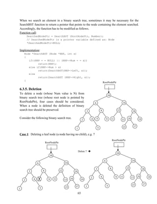
7. Advanced Sorting and Searching Algorithms
7.1. Shell Sort
Shell sort is an improvement of insertion sort. It is developed by Donald Shell in 1959. Insertion
sort works best when the array elements are sorted in a reasonable order. Thus, shell sort first
creates this reasonable order.
Algorithm:
1. Choose gap gk between elements to be partly ordered.
2. Generate a sequence (called increment sequence) gk, gk-1,…., g2, g1 where for each
sequence gi, A[j]<=A[j+gi] for 0<=j<=n-1-gi and k>=i>=1
72](https://image.slidesharecdn.com/datastructuresandalgorithmcha1and2-250314211850-11dad352/85/data-structures-and-algorithm-Cha-1and-2-doc-72-320.jpg)
![It is advisable to choose gk =n/2 and gi-1 = gi/2 for k>=i>=1. After each sequence gk-1 is done and
the list is said to be gi-sorted. Shell sorting is done when the list is 1-sorted (which is sorted
using insertion sort) and A[j]<=A[j+1] for 0<=j<=n-2. Time complexity is O(n3/2
).
Example: Sort the following list using shell sort algorithm.
5 8 2 4 1 3 9 7 6 0
Choose g3 =5 (n/2 where n is the number of elements =10)
Sort (5, 3) 3 8 2 4 1 5 9 7 6 0
Sort (8, 9) 3 8 2 4 1 5 9 7 6 0
Sort (2, 7) 3 8 2 4 1 5 9 7 6 0
Sort (4, 6) 3 8 2 4 1 5 9 7 6 0
Sort (1, 0) 3 8 2 4 0 5 9 7 6 1
5- sorted list 3 8 2 4 0 5 9 7 6 1
Choose g2 =3
Sort (3, 4, 9, 1) 1 8 2 3 0 5 4 7 6 9
Sort (8, 0, 7) 1 0 2 3 7 5 4 8 6 9
Sort (2, 5, 6) 1 0 2 3 7 5 4 8 6 9
3- sorted list 1 0 2 3 7 5 4 8 6 9
Choose g1 =1 (the same as insertion sort algorithm)
Sort (1, 0, 2, 3, 7, 5, 4, 8, 6, 9) 0 1 2 3 4 5 6 7 8 9
1- sorted (shell sorted) list 0 1 2 3 4 5 6 7 8 9
73](https://image.slidesharecdn.com/datastructuresandalgorithmcha1and2-250314211850-11dad352/85/data-structures-and-algorithm-Cha-1and-2-doc-73-320.jpg)
![7.2. Quick Sort
Quick sort is the fastest known algorithm. It uses divide and conquer strategy and in the worst
case its complexity is O (n2). But its expected complexity is O(nlogn).
Algorithm:
1. Choose a pivot value (mostly the first element is taken as the pivot value)
2. Position the pivot element and partition the list so that:
the left part has items less than or equal to the pivot value
the right part has items greater than or equal to the pivot value
3. Recursively sort the left part
4. Recursively sort the right part
The following algorithm can be used to position a pivot value and create partition.
Left=0;
Right=n-1; // n is the total number of elements in the list
PivotPos=Left;
while(Left<Right)
{
if(PivotPos==Left)
{
if(Data[Left]>Data[Right])
{
swap(data[Left], Data[Right]);
PivotPos=Right;
Left++;
}
else
Right--;
}
else
{
if(Data[Left]>Data[Right])
{
swap(data[Left], Data[Right]);
PivotPos=Left;
Right--;
}
else
Left++;
}
74](https://image.slidesharecdn.com/datastructuresandalgorithmcha1and2-250314211850-11dad352/85/data-structures-and-algorithm-Cha-1and-2-doc-74-320.jpg)


![7.3. Heap Sort
Heap sort operates by first converting the list in to a heap tree. Heap tree is a binary tree in
which each node has a value greater than both its children (if any). It uses a process called
"adjust to accomplish its task (building a heap tree) whenever a value is larger than its parent.
The time complexity of heap sort is O(nlogn).
Algorithm:
1. Construct a binary tree
The root node corresponds to Data[0].
If we consider the index associated with a particular node to be i, then the left child of this
node corresponds to the element with index 2*i+1 and the right child corresponds to the
element with index 2*i+2. If any or both of these elements do not exist in the array, then
the corresponding child node does not exist either.
2. Construct the heap tree from initial binary tree using "adjust" process.
3. Sort by swapping the root value with the lowest, right most value and deleting the
lowest, right most value and inserting the deleted value in the array in it proper position.
Example: Sort the following list using heap sort algorithm.
5 8 2 4 1 3 9 7 6 0
77
5
RootNodePtr
8
4
7
1
0
6
2
9
3
9
RootNodePtr
8
7
4
1
0
6
5
2
3
Construct the initial binary tree Construct the heap tree](https://image.slidesharecdn.com/datastructuresandalgorithmcha1and2-250314211850-11dad352/85/data-structures-and-algorithm-Cha-1and-2-doc-77-320.jpg)


data structures and algorithm Cha 1and 2.doc
- 1. Chapter-1: Data Structures and Algorithms Analysis 1.1. Introduction to Data Structures A Data Structure is a particular way of storing and organizing data in a computer so that it can be stored, retrieved, or updated efficiently. Data structures and algorithms are interrelated concepts that is the term data structure is used to describe the way data is stored, and the term algorithm is used to describe the way data is processed. In computer science, a program is written in specific programming language in order to solve a problem. A solution to a problem actually consists of two things: - A way to organize the data - Sequence of steps to solve the problem The way data are organized in a computer’s memory is said to be Data Structure; the sequence of computational steps to solve a problem is said to be an algorithm. Therefore, a program is nothing but data structures plus algorithms that is Program=Algorithm + Data structure Data structure is the building blocks of a program that should be represented in such way that it utilizes maximum efficiency. Data structure is a representation of logical relationship existing between individual elements of data. In other words, a data structure defines a way of organizing all data items that considers not only the elements stored but also their relationship to each other. Data structure is language construct that the programmer has defined in order to implement an abstract data type Used to model a problem Algorithm Specification of behavioral process Finite solution dynamic part of the world unchanged Given a problem, the first step to solve the problem is obtaining one’s own abstract view, or model, of the problem. This process of modeling is called abstraction. Abstraction is also a process of classifying characteristics as relevant and irrelevant for the particular purpose at hand and ignoring the irrelevant ones. The model defines an abstract view to the problem. This implies that the model focuses only on problem related stuff and that a programmer tries to define the properties of the problem. These properties include: - The data which are affected and - The operations that are involved in the problem. With abstraction you create a well-defined entity that can be properly handled. These entities define the data structure of the program. An entity with the properties just described is called an abstract data type (ADT). consists of data to be stored and operations supported on them describes a data the set and operation on that data An abstract data type, sometimes abbreviated ADT, is a logical description of how we view the data and the operations that are allowed without regard to how they will be implemented. This means that we are concerned only with what data is representing and not with how it will 1
- 2. eventually be constructed. By providing this level of abstraction, we are creating an encapsulation around the data. The idea is that by encapsulating the details of the implementation, we are hiding them from the user’s view. This is called information hiding. The implementation of an abstract data type, often referred to as a data structure, will require that we provide a physical view of the data using some collection of programming constructs and primitive data types. An ADT consists of an abstract data structure and operations. Put in other terms, an ADT is an abstraction of a data structure. The ADT specifies: - What can be stored in the Abstract Data Type? - What operations can be done on/by the Abstract Data Type? For example, if we are going to model employees of an organization: This ADT stores employees with their relevant attributes (EmpName, EmpID, Salary, etc) and discarding irrelevant attributes. This ADT supports hiring, firing, retiring as operations on data. Therefore, A data structure can be a language construct that the programmer has defined in order to implement an abstract data type. 1.1.1. Classifications of Data structure Data structures are broadly divided into two types: 1. Primitive data structures. 2. Non-primitive data structures 1. Primitive Data structures are basic data structure which is directly supported by the programming language ie; any operation is directly performed in these data items. Ex: integer, Character, Boolean, float, double, string, pointer etc. These primitive data structure are the basis for the discussion of more sophisticated (non-primitive) data structures. 2. Non-primitive data structures are not defined by the programming language, but are instead created by the programmer. Non primitive Data structures are more sophisticated data structure emphasizing on structuring of a group of homogenous (same type) or heterogeneous (different type) data items. Eg, Array, stack, queue, list, files, linked list, trees and graph fall in this category. Non-primitive data structures can also be categorized in to: 1. Linear data structure 2. Nonlinear data structure 1. Linear data structures: These type data structures organize their data elements in a linear fashion, where data elements are attached one after the other. They are very easy to implement, since the memory of the computer is also organized in a linear fashion. Some commonly used linear data structures are arrays, linked lists, stacks and queues. Arrays: is a collection of similar type of data items and each data item is called an element of the array. The data type of the element may be any valid data type like char, int, float or double. The elements of array share the same variable name but each one carries a different index number known as subscript. The array can be one dimensional, two dimensional or multidimensional. The individual elements of the array age are: age[0], age[1], age[2], age[3],......... age[98], age[99]. Linked List: is a linear data structure which is used to maintain a list in the memory. It can be seen as the collection of nodes stored at non-contiguous memory locations. Each node of the list contains a pointer to its adjacent node. 2
- 3. Stack: is a linear list in which insertion and deletions are allowed only at one end, called top. A stack is an abstract data type (ADT), can be implemented in most of the programming languages. It is named as stack because it behaves like a real-world stack, for example: - piles of plates or deck of cards etc. Queue: is a linear list in which elements can be inserted only at one end called rear and deleted only at the other end called front. It is an abstract data structure, similar to stack. Queue is opened at both end therefore it follows First-In-First-Out (FIFO) methodology for storing the data items. 2. Non-linear data structures: In nonlinear data structures, data elements are not organized in a sequential fashion. Data structures like trees, graphs, tables and sets are some examples of widely used nonlinear data structures. Trees: are multilevel data structures with a hierarchical relationship among its elements known as nodes. The bottommost nodes in the hierarchy are called leaf node while the topmost node is called root node. Each node contains pointers to point adjacent nodes. Tree data structure is based on the parent-child relationship among the nodes. Each node in the tree can have more than one children except the leaf nodes whereas each node can have at most one parent except the root node. Graphs: Graphs can be defined as the pictorial representation of the set of elements (represented by vertices) connected by the links known as edges. A graph is different from tree in the sense that a graph can have cycle while the tree cannot have the one. 1.1.2. Advantages of Data Structures Efficiency: Efficiency of a program depends upon the choice of data structures and there are better data structures which can make the search process efficient like ordered array, binary search tree or hash tables. Reusability: Data structures are reusable, i.e. once we have implemented a particular data structure, we can use it at any other place. Implementation of data structures can be compiled into libraries which can be used by different clients. Abstraction: Data structure is specified by the ADT which provides a level of abstraction. The client program uses the data structure through interface only, without getting into the implementation details. 1.1.3. Operations on the Data Structures: The Following common operations can be performed on the data structures: Traversing- It is used to access each data item exactly once so that it can be processed. Searching- It is used to find out the location of the data item if it exists in the given collection of data items. Inserting- It is used to add a new data item in the given collection of data items. Deleting- It is used to delete an existing data item from the given collection of data items. Sorting- It is used to arrange the data items in some order i.e. in ascending or descending order in case of numerical data and in dictionary order in case of alphanumeric data. Merging- It is used to combine the data items of two sorted files into single file in the sorted form. 1.2. Algorithms Analysis 1.2.1. Algorithm 3
- 4. An algorithm is unambiguous step-by-step instructions to solve a given problem. An algorithm is a well-defined computational procedure that takes some value or a set of values as input and produces some value or a set of values as output. Data structures model the static part of the world. They are unchanging while the world is changing. In order to model the dynamic part of the world we need to work with algorithms. Algorithms are the dynamic part of a program’s world model. An algorithm transforms data structures from one to another state in two ways: - An algorithm may change the value held by a data structure - An algorithm may change the data structure itself The quality of a data structure is related to its ability to successfully model the characteristics of the world. Similarly, the quality of an algorithm is related to its ability to successfully simulate the changes in the world. However, independent of any particular world model, the quality of data structure and algorithms is determined by their ability to work together well. Generally speaking, correct data structures lead to simple and efficient algorithms and correct algorithms lead to accurate and efficient data structures. An algorithm is a set of steps of operations to solve a problem by performing calculation, data processing, and automated reasoning tasks. It is an efficient method that can be expressed within finite amount of time and space. An algorithm is the set of instructions that describe how to solve a problem and the best way to represent the solution of a particular problem in a very simple and efficient way. If we have an algorithm for a specific problem, then we can implement it in any programming language, meaning that the algorithm is independent from any programming languages. 1.2.2. Properties of an algorithm Finiteness: Algorithm must complete after a finite number of steps. Definiteness: Each step must be clearly defined, having one and only one interpretation. At each point in computation, one should be able to tell exactly what happens next. Sequence: Each step must have a unique defined preceding and succeeding step. The first step (start step) and last step (halt step) must be clearly noted. Feasibility: It must be possible to perform each instruction. Correctness: It must compute correct answer all possible legal inputs. Language Independence: It must not depend on any one programming language. Completeness: It must solve the problem completely. Effectiveness: It must be possible to perform each step exactly & in a finite amount of time. Efficiency: It must solve with the least amount of computational resources such as time and space. Generality: Algorithm should be valid on all possible inputs. Input/Output: There must be a specified number of input values, and one or more result. Precision: the result should always be the same if the algorithm is given identical input. Simplicity: each step should carry out one logical step. What is simple to one processor may not be simple to another. Level of abstraction: used to organize the ideas expressed in algorithm, hide detail of a given activity and refer to name for those details. Simple instructions are hidden inside modules. 1.2.3. Algorithm Analysis Concepts Analysis of Algorithms is the area of computer science that provides tools to analyze the efficiency of different methods of solutions. Algorithm analysis refers to the process of 4
- 5. determining how much computing time and storage that algorithms will require. In other words, it’s a process of predicting the resource requirement of algorithms in a given environment. Why we need algorithm analysis? Writing a working program is not good enough o The program may be inefficient! o If the program is run on a large data set, then the running time becomes an issue Goal is to pick up an efficient algorithm for the problem at hand Reasons to perform analyze algorithms: It enables us to: - Predict performance of algorithms - Compare algorithms. - Provide guarantees on running time/space of algorithms - Understand theoretical basis. - Avoid performance bugs. In order to solve a problem, there are many possible algorithms. One has to be able to choose the best algorithm for the problem at hand using some scientific method. To classify some data structures and algorithms as good, we need precise ways of analyzing them in terms of resource requirement. The main resources are: Running Time Memory Usage Communication Bandwidth Running time is usually treated as the most important since computational time is the most precious resource in most problem domains. How to Measure Efficiency/performance? The performance / efficiency of algorithms can be measured on the scales of time and space. The performance of a program is the amount of computer memory and time needed to run a program. - Time efficiency (Time Complexity): is a function of the running time of the algorithm or a program. In other words, it is the amount of computer time it needs to run to completion or the computational complexity that describes the amount of time it takes to run an algorithm or program. - Space efficiency (Space Complexity): is a function of the space needed by the algorithm or program to run to completion. It is the amount of memory space required to solve an instance of the computational problem as a function of the size of the input. It is also the memory required by an algorithm to execute a program and produce output. There are two approaches to measure the efficiency of algorithms: 1. Empirical: Implement the algorithms and trying them on different instances of input and use/plot actual clock time to pick one Based on the total running time of the program. It uses actual system clock time Total time = Final time - Initial time 5
- 6. 2. Theoretical /Asymptotic analysis: Determining the quantity of resources required mathematically (Execution time, memory space, etc.) needed by each algorithm. 1. Empirical method analysis There are some drawbacks of empirical methods that it is difficult to use actual clock-time as a consistent measure of an algorithm’s efficiency, because clock-time can vary based on many things such as: Specific processor speed Current processor load Specific data for a particular run of the program (Input Size and Input Properties) Programming language Programmer Operating Environment/platform (PC, sun, smartphone etc) Operation system Multitasking vs single tasking Internal structure Therefore, it is quite machine dependent 2. Theoretical / Asymptotic analysis / Machine independent analysis. The Critical resources of the methods incudes: Time, Space (disk, RAM), Programmer’s effort, Ease of use (user’s effort). Factors affecting running time: o System dependent effects. Hardware: CPU, memory, cache, … Software: compiler, interpreter, garbage collector, … System: operating system, network, other apps, … o System independent effects Algorithm. Input data/ Problem size For most algorithms, running time depends on “size” of the input. Size is often the number of inputs processed. Example:- in searching problem, size is the no of items to be sorted. Running time is expressed as T(n) for some function T(n) on input size n. 6
- 7. The Efficiency of an algorithm is measured in terms of the number of basic operations it performs; Not based on actual time-clock. We assume that every basic operation takes constant time i.e. arbitrary time. Examples of Basic Operations: - Single Arithmetic Operation (Addition, Subtraction, Multiplication) - Assignment Operation - Single Input/output Operation - Single Boolean Operation - Function Return We do not distinguish between the basic operations. Examples of Non-basic Operations are Sorting, Searching. 1.2.4. Complexity Analysis Complexity Analysis is the systematic study of the cost of computation, measured either in time units or in operations performed, or in the amount of storage space required. The goal is to have a meaningful measure that permits comparison of algorithms independent of operating platform. There are two things to consider in complexity analysis: Time Complexity: Determine the approximate number of operations required(amount of time) to solve a problem of size n. Space Complexity: Determine the approximate memory required to solve a problem of size n. Factor affect the running time of program CPU type Memory used Computer used Programming language Algorithm used Input size Complexity analysis involves two distinct phases: Algorithm Analysis: Analysis of the algorithm or data structure to produce a function T (n) that describes the algorithm in terms of the operations performed in order to measure the complexity of the algorithm. Order of Magnitude Analysis: Analysis of the function T (n) to determine the general complexity category to which it belongs. There is no generally accepted set of rules for algorithm analysis. However, an exact count of operations is commonly used. 1.2.4.1. Analysis Rules: 1. We assume an arbitrary time unit. 2. Execution of one of the following operations takes time 1: Assignment Operation e.g. i=0 Single Input/output Operation e.g. cin>>a; Single Boolean Operations e.g. i>=10 7
- 8. Single Arithmetic Operations e.g. a+b Function Return e.g. return sum 3. Running time of a selection statement (if, switch) is the time for the condition evaluation + the maximum of the running times for the individual clauses in the selection. 4. Loops: - Running time for a loop is equal to the running time for the statements inside the loop * number of iterations. i++ n- time - The total running time of a statement inside a group of nested loops is the running time of the statements multiplied by the product of the sizes of all the loops. For nested loops, analyze from inside to out. - Always assume that the loop executes the maximum number of iterations possible. 5. Running time of a function call is 1 for setup + the time for any parameter calculations + the time required for the execution of the function body. Example 1: int cout () { int k=0; cout<< “Enter an integer”; cin>>n; for (i=0; i<n; i++) k=k+1; return 0; }6 Time Units to Compute ------------------------------------------------- 1 for the assignment statement: int k=0 1 for the output statement. 1 for the input statement. In the for loop: 1 assignment, n+1 tests, and n increments. n loops of 2 units for an assignment, and an addition. 1 for the return statement. ----------------------------------------------------- T (n)= 1+1+1+(1+n+1+n)+2n+1 = 4n+6 = O(n) Example 2 int total(int n) { int sum=0; for (int i=1;i<=n; i++) sum=sum+1; return sum; } 1+(1=n+1+n)+2n+1 Time Units to Compute ------------------------------------------------- 1 for the assignment statement: int sum=0 In the for loop: 1 assignment, n+1 tests, and n increments. n loops of 2 units for an assignment, and an addition. 1 for the return statement. ----------------------------------------------------- T (n)= 1+ (1+n+1+n)+2n+1 = 4n+4 = O(n) Example 3 void func() { int x=0; int i=0; int j=1; cout<< “Enter an Integer value”; cin>>n; while (i<n){ x++; i++; 8
- 9. } while (j<n) { j++; } } 5+n+1+n+n+n+1+n Time Units to Compute ------------------------------------------------- 1 for the first assignment statement: x=0; 1 for the second assignment statement: i=0; 1 for the third assignment statement: j=1; 1 for the output statement. 1 for the input statement. In the first while loop: n+1 test n loops of 2 units for the two increment (addition) operations In the second while loop: n tests n-1 increments? T (n)= 1+1+1+1+1+n+1+2n+n+n-1 = 5n+5 = O(n) Example 4 int sum (int n) { int partial sum = 0; for (int i = 1; i <= n; i++) partial sum = partial sum +(i * i * i); return partial sum; } Time Units to Compute ------------------------------------------------- 1 for the assignment. 1 assignment, n+1 tests, and n increments. n loops of 4 units for an assignment, an addition, and two multiplications. 1 for the return statement. ----------------------------------------------------- T (n)= 1+(1+n+1+n)+4n+1 = 6n+4 = O(n) Be careful to differentiate between: 1. Performance: how much time/memory/disk/… is actually used when a program is run. This depends on the machine, compiler, etc. as well as the code. 2. Complexity: how do the resource requirements of a program or algorithm scale, i.e., What happens, as the size of the problem being solved gets larger? 1.2.4.2. Formal Approach to Analysis In the above examples we have seen that analysis so complex. However, it can be simplified by using some formal approach in which case we can ignore initializations, loop control, and book keeping. For Loops: Formally In general, a for loop translates to a summation. The index and bounds of the summation are the same as the index and bounds of the for loop. f o r ( i n t i = 1 ; i < = N ; i + + ) { s u m = s u m + i ; } N N i 1 1 • Suppose we count the number of additions that are done. There is 1 addition per iteration of the loop, hence N additions in total. 9
- 10. Nested Loops: Formally • Nested for loops translate into multiple summations, one for each for loop. fo r (in t i =1; i < =N ; i+ + ) { for (int j =1; j < =M ; j+ + ) { sum=sum + i+ j; } } MN M N i N i M j 2 2 2 1 1 1 • Again, count the number of additions. The outer summation is for the outer for loop. Consecutive Statements: Formally • Add the running times of the separate blocks of your code for (int i = 1; i <= N ; i++) { sum = sum +i; } for (int i = 1; i <= N ; i++) { for (int j = 1; j <= N; j++) { sum = sum+i+j; } } 2 1 1 1 2 2 1 N N N i N j N i Conditionals: Formally • If (test) s1 else s2: Compute the maximum of the running time for s1 and s2. i f( t e s t= =1 ){ f o r( i n ti=1 ;i< =N ;i + + ){ s u m =s u m + i ; } } e l s ef o r( i n ti=1 ;i< =N ;i + + ){ f o r( i n tj=1 ;j< =N ;j + + ){ s u m =s u m + i + j ; } } 2 2 1 1 1 2 2 , max 2 , 1 max N N N N i N j N i Example: Suppose we have hardware capable of executing 106 instructions per second. How long would it take to execute an algorithm whose complexity function was: T (n) = 2n2 on an input size of n=108 ? The total number of operations to be performed would be T (108 ): T(108 ) = 2*(108 )2 =2*1016 10
- 11. The required number of seconds required would be given by T(108 )/106 so: Running time =2*1016 /106 = 2*1010 The number of seconds per day is 86,400 so this is about 231,480 days (634 years). Exercises Determine the run time equation and complexity of each of the following code segments. 1. for (i=0;i<n;i++) for (j=0;j<n; j++) sum=sum+i+j; What is the value of sum if n=100? T(n)=1+n+1+n+n(1+n+1+n+3n)=2n+2+n(2+5n)=5n^2+4n+2 2. for(int i=1; i<=n; i++) for (int j=1; j<=i; j++) sum++; What is the value of the sum if n=20? 3. int k=0; for (int i=0; i<n; i++) for (int j=i; j<n; j++) k++; What is the value of k when n is equal to 20? 4. int k=0; for (int i=1; i<n; i*=2) for(int j=1; j<n; j++) k++; What is the value of k when n is equal to 20? 1. int x=0; for(int i=1;i<n;i=i+5) x++; What is the value of x when n=25? 2. int x=0; for(int k=n;k>=n/3;k=k-5) x++; What is the value of x when n=25? 3. int x=0; for (int i=1; i<n;i=i+5) for (int k=n;k>=n/3;k=k-5) x++; What is the value of x when n=25? 11
- 12. 4. int x=0; for(int i=1;i<n;i=i+5) for(int j=0;j<i;j++) for(int k=n;k>=n/2;k=k-3) x++; What is the correct big-Oh Notation for the above code segment? 1.2.5. Measures of Times In order to determine the running time of an algorithm it is possible to define three functions Tbest(n), Tavg(n) and Tworst(n) as the best, the average and the Worst case running time of the algorithm respectively. Average Case (Tavg): The amount of time the algorithm takes on an "average" set of inputs. Worst Case (Tworst): The amount of time the algorithm takes on the worst possible set of inputs. Best Case (Tbest): The amount of time the algorithm takes on the smallest possible set of inputs. We are interested in the worst-case time, since it provides a bound for all input – this is called the “Big-Oh” estimate. 1.2.5. Asymptotic Analysis Order of magnitude refer to the rate at which the storage or time grows as a function of problem size Asymptotic analysis is concerned with how the running time of an algorithm increases with the size of the input in the limit, as the size of the input increases without bound. There are five notations used to describe a running time function. These are: Big-Oh Notation (O) Big-Omega Notation () Theta Notation () Little-o Notation (o) 12
- 13. Little-Omega Notation () 1.4.1. The Big-Oh Notation Big-Oh notation is a way of comparing algorithms and is used for computing the complexity of algorithms; i.e., the amount of time that it takes for computer program to run. It’s only concerned with what happens for very a large value of n. Therefore, only the largest term in the expression (function) is needed. For example, if the number of operations in an algorithm is n2 – n, n is insignificant compared to n2 for large values of n. Hence the n term is ignored. Of course, for small values of n, it may be important. However, Big-Oh is mainly concerned with large values of n. Formal Definition: f (n)= O (g (n)) if there exist c, k ∊ ℛ+ such that for all n≥ k, f (n) ≤ c.g(n). Examples: The following points are facts that you can use for Big-Oh problems: 1<=n for all n>=1 n<=n2 for all n>=1 2n <=n! for all n>=4 log2n<=n for all n>=2 n<=nlog2n for all n>=2 1. f(n)=10n+5 and g(n)=n. Show that f(n) is O(g(n)). To show that f(n) is O(g(n)) we must show that constants c and k such that f(n) <=c.g(n) for all n>=k Or 10n+5<=c.n for all n>=k Try c=15. Then we need to show that 10n+5<=15n Solving for n we get: 5<5n or 1<=n. So f(n) =10n+5 <=15.g(n) for all n>=1. (c=15,k=1). 2. f(n) = 3n2 +4n+1. Show that f(n)=O(n2 ). 4n <=4n2 for all n>=1 and 1<=n2 for all n>=1 3n2 +4n+1<=3n2 +4n2 +n2 for all n>=1 <=8n2 for all n>=1 So we have shown that f(n)<=8n2 for all n>=1 Therefore, f (n) is O(n2 ) (c=8,k=1) Typical Orders Here is a table of some typical cases. This uses logarithms to base 2, but these are simply proportional to logarithms in other base. 13
- 14. N O(1) O(log n) O(n) O(n log n) O(n2 ) O(n3 ) 1 1 1 1 1 1 1 2 1 1 2 2 4 8 4 1 2 4 8 16 64 8 1 3 8 24 64 512 16 1 4 16 64 256 4,096 1024 1 10 1,024 10,240 1,048,576 1,073,741,824 Demonstrating that a function f(n) is big-O of a function g(n) requires that we find specific constants c and k for which the inequality holds (and show that the inequality does in fact hold). Big-O expresses an upper bound on the growth rate of a function, for sufficiently large values of n. An upper bound is the best algorithmic solution that has been found for a problem. “ What is the best that we know we can do?” Exercise: f(n) = (3/2)n2 +(5/2)n-3 Show that f(n)= O(n2 ) In simple words, f (n) =O(g(n)) means that the growth rate of f(n) is less than or equal to g(n). 1.4.1.1. Big-O Theorems For all the following theorems, assume that f(n) is a function of n and that k is an arbitrary constant. Theorem 1: k is O(1) Theorem 2: A polynomial is O(the term containing the highest power of n). Polynomial’s growth rate is determined by the leading term If f(n) is a polynomial of degree d, then f(n) is O(nd ) In general, f(n) is big-O of the dominant term of f(n). Theorem 3: k*f(n) is O(f(n)) Constant factors may be ignored E.g. f(n) =7n4 +3n2 +5n+1000 is O(n4 ) Theorem 4(Transitivity): If f(n) is O(g(n)) and g(n) is O(h(n)), then f(n) is O(h(n)). Theorem 5: For any base b, logb(n) is O(logn). All logarithms grow at the same rate logbn is O (logd n) b, d > 1 14
- 15. Theorem 6: Each of the following functions is big-O of its successors: k logbn n nlogbn n2 n to higher powers 2n 3n larger constants to the nth power n! nn f(n)= 3nlogbn + 4 logbn+2 is O(nlogbn) and )(n2 ) and O(2n ) 1.4.1.2. Properties of the O Notation Higher powers grow faster • nr is O( ns ) if 0 <= r <= s Fastest growing term dominates a sum • If f(n) is O(g(n)), then f(n) + g(n) is O(g) E.g 5n4 + 6n3 is O (n4 ) Exponential functions grow faster than powers, i.e. is O( bn ) b > 1 and k >= 0 E.g. n20 is O( 1.05n ) Logarithms grow more slowly than powers • logbn isO( nk) b > 1 and k >= 0 E.g. log2n is O( n0.5 ) 1.4.2. Big-Omega Notation Just as O-notation provides an asymptotic upper bound on a function, notation provides an asymptotic lower bound. Formal Definition: A function f(n) is ( g (n)) if there exist constants c and k ∊ ℛ+ such that f(n) >=c. g(n) for all n>=k. f(n)= ( g (n)) means that f(n) is greater than or equal to some constant multiple of g(n) for all values of n greater than or equal to some k. Example: If f(n) =n2, then f(n)= ( n) In simple terms, f(n)= ( g (n)) means that the growth rate of f(n) is greater that or equal to g(n). 1.4.3. Theta Notation A function f (n) belongs to the set of (g(n)) if there exist positive constants c1 and c2 such that it can be sandwiched between c1.g(n) and c2.g(n), for sufficiently large values of n. 15
- 16. Formal Definition: A function f (n) is (g(n)) if it is both O( g(n) ) and ( g(n) ). In other words, there exist constants c1, c2, and k >0 such that c1.g (n)<=f(n)<=c2. g(n) for all n >= k If f(n)= (g(n)), then g(n) is an asymptotically tight bound for f(n). In simple terms, f(n)= (g(n)) means that f(n) and g(n) have the same rate of growth. Example: 1. If f(n)=2n+1, then f(n) = (n) 2. f(n) =2n2 then f(n)=O(n4 ) f(n)=O(n3 ) f(n)=O(n2 ) All these are technically correct, but the last expression is the best and tight one. Since 2n2 and n2 have the same growth rate, it can be written as f(n)= (n2 ). 1.4.4. Little-o Notation Big-Oh notation may or may not be asymptotically tight, for example: 2n2 = O(n2 ) =O(n3 ) f(n)=o(g(n)) means for all c>0 there exists some k>0 such that f(n)<c.g(n) for all n>=k. Informally, f(n)=o(g(n)) means f(n) becomes insignificant relative to g(n) as n approaches infinity. Example: f(n)=3n+4 is o(n2 ) In simple terms, f(n) has less growth rate compared to g(n). g(n)= 2n2 g(n) =o(n3 ), O(n2 ), g(n) is not o(n2 ). 1.4.5. Little-Omega ( notation) Little-omega () notation is to big-omega () notation as little-o notation is to Big-Oh notation. We use notation to denote a lower bound that is not asymptotically tight. Formal Definition: f(n)= (g(n)) if there exists a constant no>0 such that 0<= c. g(n)<f(n) for all n>=k. Example: 2n2 =(n) but it’s not (n). 1.5. Relational Properties of the Asymptotic Notations Transitivity • if f(n)=(g(n)) and g(n)= (h(n)) then f(n)=(h(n)), • if f(n)=O(g(n)) and g(n)= O(h(n)) then f(n)=O(h(n)), • if f(n)=(g(n)) and g(n)= (h(n)) then f(n)= (h(n)), • if f(n)=o(g(n)) and g(n)= o(h(n)) then f(n)=o(h(n)), and • if f(n)= (g(n)) and g(n)= (h(n)) then f(n)= (h(n)). 16
- 17. Symmetry • f(n)=(g(n)) if and only if g(n)=(f(n)). Transpose symmetry • f(n)=O(g(n)) if and only if g(n)=(g(n), • f(n)=o(g(n)) if and only if g(n)=(g(n)). Reflexivity • f(n)=(f(n)), • f(n)=O(f(n)), • f(n)=(f(n)). 17
- 18. Chapter 2. Simple Sorting and Searching Algorithms 2.1. Searching Searching is a process of looking for a specific element in a list of items or determining that the item is not in the list. There are two simple searching algorithms: • Sequential Search, and • Binary Search 2.1.1. Linear Search (Sequential Search) Pseudocode Loop through the array starting at the first element until the value of target matches one of the array elements. If a match is not found, return –1. Time is proportional to the size of input (n) and we call this time complexity O(n) . Example Implementation: int Linear_Search(int list[], int key) { int index=0; int found=0; do{ if(key==list[index]) found=1; else index++; }while(found==0&&index<n); if(found==0) index=-1; return index; } 2.1.2. Binary Search This searching algorithm works only on an ordered list: Pseudocode
- 19. • Locate midpoint of array to search • Determine if target is in lower half or upper half of an array. o If in lower half, make this half the array to search o If in the upper half, make this half the array to search • Loop back to step 1 until the size of the array to search is one, and this element does not match, in which case return –1. The computational time for this algorithm is proportional to log2 n . Therefore the time complexity is O(log n) Example Implementation: int Binary_Search(int list[],int k) { int left=0; int right=n-1; int found=0; do{ mid=(left+right)/2; if(key==list[mid]) found=1; else{ if(key<list[mid]) right=mid-1; else left=mid+1; } }while(found==0&&left<right); if(found==0) index=-1; else index=mid; return index; } 2.2. Sorting Algorithms Sorting is one of the most important operations performed by computers. Sorting is a process of reordering a list of items in either increasing or decreasing order. The following are simple sorting algorithms used to sort small-sized lists. • Insertion Sort
- 20. • Selection Sort • Bubble Sort
- 21. 2.2.1. Insertion Sort The insertion sort works just like its name suggests - it inserts each item into its proper place in the final list. The simplest implementation of this requires two list structures - the source list and the list into which sorted items are inserted. To save memory, most implementations use an in- place sort that works by moving the current item past the already sorted items and repeatedly swapping it with the preceding item until it is in place. It's the most instinctive type of sorting algorithm. The approach is the same approach that you use for sorting a set of cards in your hand. While playing cards, you pick up a card, start at the beginning of your hand and find the place to insert the new card, insert it and move all the others up one place. Basic Idea: Find the location for an element and move all others up, and insert the element. The process involved in insertion sort is as follows: 1. The left most value can be said to be sorted relative to itself. Thus, we don’t need to do anything. 2. Check to see if the second value is smaller than the first one. If it is swap these two values. The first two values are now relatively sorted. 3. Next, we need to insert the third value in to the relatively sorted portion so that after insertion, the portion will still be relatively sorted. 4. Remove the third value first. Slide the second value to make room for insertion. Insert the value in the appropriate position. 5. Now the first three are relatively sorted. 6. Do the same for the remaining items in the list. Implementation void insertion_sort(int list[]){ int temp; for(int i=1;i<n;i++){ temp=list[i]; for(int j=i; j>0 && temp<list[j-1];j--) { // work backwards through the array finding where temp should go list[j]=list[j-1]; list[j-1]=temp; }//end of inner loop }//end of outer loop }//end of insertion_sort Analysis The body of insertion_sort is made up of two nested for loops. The outer for
- 22. loop is executed n - 1 times.i.e: How many comparisons? 1+2+3+…+(n-1)= O(n2 ) For the inner for loop is the total number of comparisons will be(Counting comparisons or swaps yields similar results.) How many swaps? 1+2+3+…+(n-1)= O(n2 ) How much space? In-place algorithm 2.2.2. Selection Sort Basic Idea: Loop through the array from i=0 to n-1. Select the smallest element in the array from I to n Swap this value with value at position i. Implementation: void selection_sort(int list[]) { int i,j, smallest; for(i=0;i<n;i++){ smallest=i; for(j=i+1;j<n;j++){ if(list[j]<list[smallest]) smallest=j; }//end of inner loop temp=list[smallest]; list[smallest]=list[i]; list[i]=temp; } //end of outer loop }//end of selection_sort Analysis Selection Sort first finds the smallest key in an unsorted list, then the second smallest, and so on. Its unique feature is that there are few record swaps. To find the next smallest key value requires searching through the entire unsorted portion of the array, but only one swap is required to put the record in place. Thus, the total number of swaps required will be n-1.
- 23. How many comparisons? (n-1)+(n-2)+…+1= O(n2 ) How many swaps? n=O(n) How much space? In-place algorithm 2.2.3. Bubble Sort Bubble Sort consists of a simple double for loop. The first iteration of the inner for loop moves through the record array from bottom to top, comparing adjacent keys. If the lower-indexed key’s value is greater than its higher-indexed neighbor, then the two values are swapped. Once the smallest value is encountered, this process will cause it to “bubble” up to the top of the array. The second pass through the array repeats this process. Bubble sort is the simplest algorithm to implement and the slowest algorithm on very large inputs. Basic Idea: Loop through array from i=0 to n and swap adjacent elements if they are out of order. Implementation: void bubble_sort(list[]) { int i,j; for(int i=0;i<n; i++){ for(j=n-1;j>i; j--){ if(list[j]<list[j-1]){ temp=list[j]; list[j]=list[j-1]; list[j-1]=temp; }//swap adjacent elements }//end of inner loop }//end of outer loop }//end of bubble_sort Analysis of Bubble Sort How many comparisons?
- 24. (n-1)+(n-2)+…+1= O(n2 ) How many swaps? (n-1)+(n-2)+…+1= O(n2 ) Space? In-place algorithm. General Comments Each of these algorithms requires n-1 passes: each pass places one item in its correct place. The ith pass makes either i or n - i comparisons and moves. So: or O(n2 ). Thus these algorithms are only suitable for small problems where their simple code makes them faster than the more complex code of the O(n logn) algorithm. As a rule of thumb, expect to find an O(n logn) algorithm faster for n>10 - but the exact value depends very much on individual machines!. Empirically it’s known that Insertion sort is over twice as fast as the bubble sort and is just as easy to implement as the selection sort. In short, there really isn't any reason to use the selection sort - use the insertion sort instead. If you really want to use the selection sort for some reason, try to avoid sorting lists of more than a 1000 items with it or repetitively sorting lists of more than a couple hundred items.
- 25. Chapter 3. Data Structures 3.1. Structures Structures are aggregate data types built using elements of primitive data types. struct Time{ int hour; int minute; int second; }; The struct keyword creates a new user defined data type that is used to declare variables of an aggregate data type. Structure variables are declared like variables of other types. Syntax: struct <structure tag> <variable name>; E.g. struct Time timeObject, struct Time *timeptr; 3.1.1. Accessing Members of Structure Variables The Dot operator (.): to access data members of structure variables. The Arrow operator (->): to access data members of pointer variables pointing to the structure. E.g. Print member hour of timeObject and timeptr. cout<< timeObject.hour; or cout<<timeptr->hour; TIP: timeptr->hour is the same as (*timeptr).hour. The parentheses is required since (*) has lower precedence than (.). 3.1.2. Self-Referential Structures Structures can hold pointers to instances of themselves. struct list{ char name[10]; int count; struct list *next; }; However, structures cannot contain instances of themselves. 3.2. Linked Lists Linked lists are the most basic self-referential structures. Linked lists allow you to have a chain of structs with related data.
- 26. Array Vs. Linked lists Arrays are simple and fast but we must specify their size at construction time. This has its own drawbacks. If you construct an array with space for n, tomorrow you may need n+1.Here comes a need for a more flexible system? Advantages of Linked Lists Flexible space use by dynamically allocating space for each element as needed. This implies that one need not now the size of the list in advance. Memory is efficiently utilized. A linked list is made up of a chain of nodes. Each node contains: • the data item, and • a pointer to the next node 3.2.1. Declaring a Linked list It involves a struct and a pointer: struct list_node { <type> data; struct list_node *next; }; Another way is using typedef: typedef struct list_node { <type> data; struct list_node *next; } node; node *head = NULL; Note: Node is a type specifier and not a structure variable. Even the typedef is specified, the next pointer within the struct must still have the struct tag! 3.2.2. Creating Linked Lists in C++ A linked list is a data structure that is built from structures and pointers. It forms a chain of "nodes" with pointers representing the links of the chain and holding the entire thing together. A linked list can be represented by a diagram like this one:
- 27. This linked list has four nodes in it, each with a link to the next node in the series. The last node has a link to the special value NULL, which any pointer (whatever its type) can point to, to show that it is the last link in the chain. There is also another special pointer, called Start (also called head), which points to the first link in the chain so that we can keep track of it. 3.2.3. Defining the data structure for a linked list The key part of a linked list is a structure, which holds the data for each node (the name, address, age or whatever for the items in the list), and, most importantly, a pointer to the next node. Here we have given the structure of a typical node: struct node { char name[20]; // Name of up to 20 letters int age float height; // In metres node *nxt;// Pointer to next node }; node *start_ptr = NULL; The important part of the structure is the line before the closing curly brackets. This gives a pointer to the next node in the list. This is the only case in C++ where you are allowed to refer to a data type (in this case node) before you have even finished defining it! We have also declared a pointer called start_ptr that will permanently point to the start of the list. To start with, there are no nodes in the list, which is why start_ptr is set to NULL. 3.2.4. Adding a node to the end of the list The first problem that we face is how to add a node to the list. For simplicity's sake, we will assume that it has to be added to the end of the list, although it could be added anywhere in the list (a problem we will deal with later on). Firstly, we declare the space for a pointer item and assign a temporary pointer to it. This is done using the new statement as follows: temp = new node; We can refer to the new node as *temp, i.e. "the node that temp points to". When the fields of this structure are referred to, brackets can be put round the *temp part, as otherwise the compiler will think we are trying to refer to the fields of the pointer. Alternatively, we can use the arrow pointer notation.
- 28. That's what we shall do here. Having declared the node, we ask the user to fill in the details of the person, i.e. the name, age, height or whatever is defined at the structure(struct node): cout << "Please enter the name of the person: "; cin >> temp->name; cout << "Please enter the age of the person : "; cin >> temp->age; cout << "Please enter the height of the person : "; cin >> temp->height; temp->nxt = NULL; The last line sets the pointer from this node to the next to NULL, indicating that this node, when it is inserted in the list, will be the last node. Having set up the information, we have to decide what to do with the pointers. Of course, if the list is empty to start with, there's no problem - just set the Start pointer to point to this node (i.e. set it to the same value as temp): if (start_ptr == NULL) start_ptr = temp; It is harder if there are already nodes in the list. In this case, the secret is to declare a second pointer, temp2, to step through the list until it finds the last node. temp2 = start_ptr; // We know this is not NULL - list not empty! while (temp2->nxt != NULL) { temp2 = temp2->nxt; // Move to next link in chain }
- 29. delete temp; // Wipe out original start node Here is the function that deletes a node from the start: void delete_start_node() { node *temp; temp = start_ptr; start_ptr = start_ptr->nxt; delete temp; } Deleting a node from the end of the list is harder, as the temporary pointer must find where the end of the list is by hopping along from the start. This is done using code that is almost identical to that used to insert a node at the end of the list. It is necessary to maintain two temporary pointers, temp1 and temp2. The pointer temp1 will point to the last node in the list and temp2 will point to the previous node. We have to keep track of both as it is necessary to delete the last node and immediately afterwards, to set the nxt pointer of the previous node to NULL (it is now the new last node). 1. Look at the start pointer. If it is NULL, then the list is empty, so print out a "No nodes to delete" message. 2. Make temp1 point to whatever the start pointer is pointing to. 3. If the nxt pointer of what temp1 indicates is NULL, then we've found the last node of the list, so jump to step 7. 4. Make another pointer, temp2, point to the current node in the list.
- 30. 5. Make temp1 point to the next item in the list. 6. Go to step 3. 7. If you get this far, then the temporary pointer, temp1, should point to the last item in the list and the other temporary pointer, temp2, should point to the last-but-one item. 8. Delete the node pointed to by temp1. 9. Mark the nxt pointer of the node pointed to by temp2 as NULL - it is the new last node. Let's try it with a rough drawing. This is always a good idea when you are trying to understand an abstract data type. Suppose we want to delete the last node from this list: Firstly, the start pointer doesn't point to NULL, so we don't have to display a "Empty list, wise guy!" message. Let's get straight on with step2 - set the pointer temp1 to the same as the start pointer: The nxt pointer from this node isn't NULL, so we haven't found the end node. Instead, we set the pointer temp2 to the same node as temp1 and then move temp1 to the next node in the list:
- 31. Going back to step 3, we see that temp1 still doesn't point to the last node in the list, so we make temp2 point to what temp1 points to and temp1 is made to point to the next node along: Eventually, this goes on until temp1 really is pointing to the last node in the list, with temp2 pointing to the penultimate node: NULL temp 2 temp1 start_ptr NULL temp 2 temp1 start_ptr
- 32. Now we have reached step 8. The next thing to do is to delete the node pointed to by temp1 and set the nxt pointer of what temp2 indicates to NULL: We suppose you want some code for all that! All right then .... void delete_end_node() { node *temp1, *temp2; if (start_ptr == NULL) cout << "The list is empty!" << endl; else { temp1 = start_ptr; while (temp1->nxt != NULL) { temp2 = temp1; temp1 = temp1->nxt; } delete temp1; temp2->nxt = NULL; } } The code seems a lot shorter than the explanation! Now, the sharp-witted amongst you will have spotted a problem. If the list only contains one node, the code above will malfunction. This is because the function goes as far as the temp1 = start_ptr statement, but never gets as far as setting up temp2. The code above has to be adapted so that if the first node is also the last (has a NULL nxt pointer), then it is deleted and the start_ptr pointer is assigned to NULL. In this case, there is no need for the pointer temp2:
- 33. void delete_end_node() { node *temp1, *temp2; if (start_ptr == NULL) cout << "The list is empty!" << endl; else { temp1 = start_ptr; if (temp1->nxt == NULL) // This part is new! { delete temp1; start_ptr = NULL; } else { while (temp1->nxt != NULL) { temp2 = temp1; temp1 = temp1->nxt; } delete temp1; temp2->nxt = NULL; } } } 3.2.5. Navigating through the list One thing you may need to do is to navigate through the list, with a pointer that moves backwards and forwards through the list, like an index pointer in an array. This is certainly necessary when you want to insert or delete a node from somewhere inside the list, as you will need to specify the position. We will call the mobile pointer current. First of all, it is declared, and set to the same value as the start_ptr pointer: node *current; current = start_ptr; Notice that you don't need to set current equal to the address of the start pointer, as they are both pointers. The statement above makes them both point to the same thing:
- 34. It's easy to get the current pointer to point to the next node in the list (i.e. move from left to right along the list). If you want to move current along one node, use the nxt field of the node that it is pointing to at the moment: current = current->nxt; In fact, we had better check that it isn't pointing to the last item in the list. If it is, then there is no next node to move to: if (current->nxt == NULL) cout << "You are at the end of the list." << endl; else current = current->nxt; Moving the current pointer back one step is a little harder. This is because we have no way of moving back a step automatically from the current node. The only way to find the node before the current one is to start at the beginning, work our way through and stop when we find the node before the one we are considering the moment. We can tell when this happens, as the nxt pointer from that node will point to exactly the same place in memory as the current pointer (i.e. the current node). First of all, we had better check to see if the current node is also first the one. If it is, then there is no "previous" node to point to. If not, check through all the nodes in turn until we detect that we are just behind the current one (Like a pantomime - "behind you!") if (current == start_ptr) cout << "You are at the start of the list" << endl; else { node *previous; // Declare the pointer previous = start_ptr; NULL previous current Start Stop here
- 35. while (previous->nxt != current) { previous = previous->nxt; } current = previous; } The else clause translates as follows: Declare a temporary pointer (for use in this else clause only). Set it equal to the start pointer. All the time that it is not pointing to the node before the current node, move it along the line. Once the previous node has been found, the current pointer is set to that node - i.e. it moves back along the list. Now that you have the facility to move back and forth, you need to do something with it. Firstly, let's see if we can alter the details for that particular node in the list: cout << "Please enter the new name of the person: "; cin >> current->name; cout << "Please enter the new age of the person : "; cin >> current->age; cout << "Please enter the new height of the person : "; cin >> current->height; The next easiest thing to do is to delete a node from the list directly after the current position. We have to use a temporary pointer to point to the node to be deleted. Once this node has been "anchored", the pointers to the remaining nodes can be readjusted before the node on death row is deleted. Here is the sequence of actions: 1. Firstly, the temporary pointer is assigned to the node after the current one. This is the node to be deleted: 2. Now the pointer from the current node is made to leap-frog the next node and point to the one after that: NULL current temp current temp NULL
- 36. 3. The last step is to delete the node pointed to by temp. Here is the code for deleting the node. It includes a test at the start to test whether the current node is the last one in the list: if (current->nxt == NULL) cout << "There is no node after current" << endl; else { node *temp; temp = current->nxt; current->nxt = temp->nxt; // Could be NULL delete temp; } Here is the code to add a node after the current one. This is done similarly, but we haven't illustrated it with diagrams: if (current->nxt == NULL) add_node_at_end(); else { node *temp; new temp; get_details(temp); // Make the new node point to the same thing as // the current node temp->nxt = current->nxt; // Make the current node point to the new link // in the chain current->nxt = temp; } We have assumed that the function add_node_at_end() is the routine for adding the node to the end of the list that we created near the top of this section. This routine is called if the current pointer is the last one in the list so the new one would be added on to the end.
- 37. Similarly, the routine get_temp(temp) is a routine that reads in the details for the new node similar to the one defined just above. ... and so ... 3.3. Doubly Linked Lists That sounds even harder than a linked list! Well, if you've mastered how to do ordinary linked lists, then it shouldn't be much of a leap to doubly linked lists. It's like climbing Everest - very difficult, but if you've already climbed Snowdon, Kilimanjaro and K2, then it doesn't seem so fearsome! A doubly linked list is one where there are links from each node in both directions: You will notice that each node in the list has two pointers, one to the next node and one to the previous one - again, the ends of the list are defined by NULL pointers. Also there is no pointer to the start of the list. Instead, there is simply a pointer to some position in the list which can be moved left or right. The reason we needed a start pointer in the ordinary linked list is because, having moved on from one node to another, we can't easily move back ("The moving pointer doth write, and having writ, moves on!") so without the start pointer, we would lose track of all the nodes in the list that we have already passed. With the doubly linked list, we can move the current pointer backwards and forwards at will. The nodes for a doubly linked list would be defined as follows: struct node { string name; node *nxt; // Pointer to next node node *prv; // Pointer to previous node }; node *current; current = new node;
- 38. current->name = "Fred"; current->nxt = NULL; current->prv = NULL; I have also included some code to declare the first node and set its pointers to NULL. It gives the following situation: We still need to consider the directions 'forward' and 'backward', so in this case, we will need to define functions to add a node to the start of the list (left-most position) and the end of the list (right-most position): void add_node_at_start (string new_name) { // Declare a temporary pointer and move it to the start node *temp = current; while (temp->prv != NULL) temp = temp->prv; // Declare a new node and link it in node *temp2; temp2 = new node; temp2->name = new_name; // Store the new name in the node temp2->prv = NULL; // This is the new start of the list temp2->nxt = temp; // Links to current list temp->prv = temp2; } void add_node_at_end () { // Declare a temporary pointer and move it to the end node *temp = current; while (temp->nxt != NULL) temp = temp->nxt;
- 39. // Declare a new node and link it in node *temp2; temp2 = new node; temp2->name = new_name; // Store the new name in the node temp2->nxt = NULL; // This is the new start of the list temp2->prv = temp; // Links to current list temp->nxt = temp2; } Here, the new name is passed to the appropriate function as a parameter. I'll go through the function for adding a node to the right-most end of the list. The method is similar for adding a node at the other end. Firstly, a temporary pointer is set up and is made to march along the list until it points to last node in the list. After that, a new node is declared, and the name is copied into it. The nxt pointer of this new node is set to NULL to indicate that this node will be the new end of the list. The prv pointer of the new node is linked into the last node of the existing list. The nxt pointer of the current end of the list is set to the new node.
- 40. Chapter 4. Stacks A simple data structure in which insertion and deletion occur at the same end, is termed (called) a stack. It is a LIFO (Last In First Out) structure. The operations of insertion and deletion are called PUSH and POP Push - push (put) item onto stack Pop - pop (get) item from stack Initial Stack Push(8) Pop TOS=> 4 1 3 6 TOS=> 8 4 1 3 6 TOS=> 4 1 3 6 Our Purpose: To develop a stack implementation that does not tie us to a particular data type or to a particular implementation. Implementation: Stacks can be implemented both as an array (contiguous list) or as a linked list. We want a set of operations that will work with either type of implementation: i.e. the method of implementation is hidden and can be changed without affecting the programs that use them. The Basic Operations: Push() { if there is room { put an item on the top of the stack else give an error message } }
- 41. Pop() { if stack not empty { return the value of the top item remove the top item from the stack } else { give an error message } } CreateStack() { remove existing items from the stack initialise the stack to empty } 4.1 Array Implementation of Stacks: The PUSH operation Here, as you might have noticed, addition of an element is known as the PUSH operation. So, if an array is given to you, which is supposed to act as a STACK, you know that it has to be a STATIC Stack; meaning, data will overflow if you cross the upper limit of the array. So, keep this in mind. Algorithm: Step-1: Increment the Stack TOP by 1. Check whether it is always less than the Upper Limit of the stack. If it is less than the Upper Limit go to step-2 else report -"Stack Overflow" Step-2: Put the new element at the position pointed by the TOP Implementation: static int stack[UPPERLIMIT]; int top= -1; /*stack is empty*/ .. .. main() { .. .. push(item); .. .. } push(int item) {
- 42. top = top + 1; if(top < UPPERLIMIT) stack[top] = item; /*step-1 & 2*/ else cout<<"Stack Overflow"; } Note:- In array implementation,we have taken TOP = -1 to signify the empty stack, as this simplifies the implementation. 4.2 Array Implementation of Stacks: the POP operation POP is the synonym for delete when it comes to Stack. So, if you're taking an array as the stack, remember that you'll return an error message, "Stack underflow", if an attempt is made to Pop an item from an empty Stack. OK. Algorithm Step-1: If the Stack is empty then give the alert "Stack underflow" and quit; or else go to step-2 Step-2: a) Hold the value for the element pointed by the TOP b) Put a NULL value instead c) Decrement the TOP by 1 Implementation: static int stack[UPPPERLIMIT]; int top=-1; .. .. main() { .. .. poped_val = pop(); .. .. } int pop() { int del_val = 0; if(top == -1) cout<<"Stack underflow"; /*step-1*/ else {
- 43. del_val = stack[top]; /*step-2*/ stack[top] = NULL; top = top -1; } return(del_val); } Note: - Step-2:(b) signifies that the respective element has been deleted. Algorithm Step-1: If the Stack is empty go to step-2 or else go to step-3 Step-2: Create the new element and make your "stack" and "top" pointers point to it and quit. Step-3: Create the new element and make the last (top most) element of the stack to point to it Step-4: Make that new element your TOP most element by making the "top" pointer point to it. Implementation: struct node { int item; struct node *next; } struct node *stack = NULL; /*stack is initially empty*/ struct node *top = stack; main() { .. .. push(item); .. } push(int item) { if(stack == NULL) /*step-1*/ { newnode = new node /*step-2*/ newnode -> item = item; newnode -> next = NULL; stack = newnode; top = stack; } else { newnode = new node; /*step-3*/ newnode -> item = item; newnode -> next = NULL; top ->next = newnode; top = newnode; /*step-4*/
- 44. } } 4.3 Linked List Implementation of Stacks: the PUSH operation It’s very similar to the insertion operation in a dynamic singly linked list. The only difference is that here you'll add the new element only at the end of the list, which means addition can happen only from the TOP. Since a dynamic list is used for the stack, the Stack is also dynamic, means it has no prior upper limit set. So, we don't have to check for the Overflow condition at all! In Step [1] we create the new element to be pushed to the Stack. In Step [2] the TOP most element is made to point to our newly created element. In Step [3] the TOP is moved and made to point to the last element in the stack, which is our newly added element. 4.4 Linked List Implementation of Stacks: the POP Operation This is again very similar to the deletion operation in any Linked List, but you can only delete from the end of the list and only one at a time; and that makes it a stack. Here, we'll have a list pointer, "target", which will be pointing to the last but one element in the List (stack). Every time we POP, the TOP most element will be deleted and "target" will be made as the TOP most element. In step[1] we got the "target" pointing to the last but one node. In step[2] we freed the TOP most element. In step[3] we made the "target" node as our TOP most element. Supposing you have only one element left in the Stack, then we won't make use of "target" rather we'll take help of our "bottom" pointer. See how... Algorithm: Step-1: If the Stack is empty then give an alert message "Stack Underflow" and quit; or else proceed Step-2: If there is only one element left go to step-3 or else step-4 Step-3: Free that element and make the "stack", "top" and "bottom" pointers point to NULL and quit Step-4: Make "target" point to just one element before the TOP; free the TOP most element; make "target" as your TOP most element Implementation: struct node { int nodeval; struct node *next; }
- 45. struct node *stack = NULL; /*stack is initially empty*/ struct node *top = stack; main() { int newvalue, delval; .. push(newvalue); .. delval = pop(); /*POP returns the deleted value from the stack*/ } int pop( ) { int pop_val = 0; struct node *target = stack; if(stack == NULL) /*step-1*/ cout<<"Stack Underflow"; else { if(top == bottom) /*step-2*/ { pop_val = top -> nodeval; /*step-3*/ delete top; stack = NULL; top = bottom = stack; } else /*step-4*/ { while(target->next != top) target = target ->next; pop_val = top->nodeval; delete top; top = target; target ->next = NULL; } } return(pop_val); } 4.5 Applications of Stacks 4.5.1 Evaluation of Algebraic Expressions Example: 4 + 5 * 5 Simple calculator: 45 Scientific calculator: 29 (correct) Question: Can we develop a method of evaluating arithmetic expressions without having to ‘look ahead’ or ‘look back’? ie consider the quadratic formula:
- 46. x = (-b+(b^2-4*a*c)^0.5)/(2*a) where ^ is the power operator, or, as you may remember it : In it’s current form we cannot solve the formula without considering the ordering of the parentheses. i.e. we solve the innermost parenthesis first and then work outwards also considering operator precedence. Although we do this naturally, consider developing an algorithm to do the same . . . . . . possible but complex and inefficient. Instead . . . . Re-expressing the Expression Computers solve arithmetic expressions by restructuring them so the order of each calculation is embedded in the expression. Once converted an expression can then be solved in one pass. Types of Expression The normal (or human) way of expressing mathematical expressions is called infix form, e.g. 4+5*5. However, there are other ways of representing the same expression, either by writing all operators before their operands or after them, e.g.: 4 5 5 * + + 4 * 5 5 This method is called Polish Notation (because this method was discovered by the Polish mathematician Jan Lukasiewicz). When the operators are written before their operands, it is called the prefix form Example: + 4 * 5 5 When the operators come after their operands, it is called postfix form (suffix form or reverse polish notation) Example: 4 5 5 * + The valuable aspect of RPN (Reverse Polish Notation or postfix ) Parentheses are unnecessary Easy for a computer (compiler) to evaluate an arithmetic expression Postfix (Reverse Polish Notation) Postfix notation arises from the concept of post-order traversal of an expression tree (see Weiss p. 93 - this concept will be covered when we look at trees). For now, consider postfix notation as a way of redistributing operators in an expression so that their operation is delayed until the correct time. Consider again the quadratic formula:
- 47. x = (-b+(b^2-4*a*c)^0.5)/(2*a) In postfix form the formula becomes: x b @ b 2 ^ 4 a * c * - 0.5 ^ + 2 a * / = where @ represents the unary - operator. Notice the order of the operands remain the same but the operands are redistributed in a non- obvious way (an algorithm to convert infix to postfix can be derived). Purpose The reason for using postfix notation is that a fairly simple algorithm exists to evaluate such expressions based on using a stack: Postfix Evaluation Consider the postfix expression: 6 5 2 3 + 8 * + 3 + * Algorithm initialise stack to empty; while (not end of postfix expression) { get next postfix item; if(item is value) push it onto the stack; else if(item is binary operator) { pop the stack to x; pop the stack to y; perform y operator x; push the results onto the stack; } else if (item is unary operator) { pop the stack to x; perform operator(x); push the results onto the stack } } The single value on the stack is the desired result. Binary operators: +, -, *, /, etc., Unary operators: unary minus, square root, sin, cos, exp, etc., So for 6 5 2 3 + 8 * + 3 + *
- 48. The first item is a value (6) so it is pushed onto the stack The next item is a value (5) so it is pushed onto the stack The next item is a value (2) so it is pushed onto the stack The next item is a value (3) so it is pushed onto the stack and the stack becomes TOS=> 3 2 5 6 the remaining items are now: + 8 * + 3 + * So next a '+' is read (a binary operator), so 3 and 2 are popped from the stack and their sum '5' is pushed onto the stack: TOS=> 5 5 6 Next 8 is pushed and the next item is the operator *: TOS=> 8 5 TOS=> 40
- 49. 5 6 5 6 (8, 5 popped, 40 pushed) Next the operator + followed by 3: TOS=> 45 6 TOS=> 3 45 6 (40, 5 popped, 45 pushed, 3 pushed) Next is operator +, so 3 and 45 are popped and 45+3=48 is pushed TOS=> 48 6 Next is operator *, so 48 and 6 are popped, and 6*48=288 is pushed
- 50. TOS=> 288 Now there are no more items and there is a single value on the stack, representing the final answer 288. Note the answer was found with a single traversal of the postfix expression, with the stack being used as a kind of memory storing values that are waiting for their operands. 4.5.2 Function Calls When a function is called, arguments (including the return address) have to be passed to the called function. If these arguments are stored in a fixed memory area then the function can not be called recursively since the 1st return address would be overwritten by the 2nd return address before the first was used: 10 call function abc(); /* retadrs = 11 */ 11 continue; ... 90 function abc; 91 code; 92 if (expression) 93 call function abc(); /* retadrs = 94 */ 94 code 95 return /* to retadrs */ A stack allows a new instance of retadrs for each call to the function. Recursive calls on the function are limited only by the extent of the stack. 10 call function abc(); /* retadrs1 = 11 */ 11 continue; ... 90 function abc; 91 code; 92 if (expression) 93 call function abc(); /* retadrs2 = 94 */ 94 code
- 51. 95 return /* to retadrsn */
- 52. Chapter 5. Queues a data structure that has access to its data at the front and rear. operates on FIFO (Fast In First Out) basis. uses two pointers/indices to keep tack of information/data. has two basic operations: o enqueue - inserting data at the rear of the queue o dequeue – removing data at the front of the queue Example: Operation Content of queue Enqueue(B) B Enqueue(C) B, C Dequeue() C Enqueue(G) C, G Enqueue (F) C, G, F Dequeue() G, F Enqueue(A) G, F, A Dequeue() F, A 5.1. Simple array implementation of enqueue and dequeue operations Analysis: Consider the following structure: int Num[MAX_SIZE]; We need to have two integer variables that tell: - the index of the front element - the index of the rear element We also need an integer variable that tells: - the total number of data in the queue int FRONT =-1,REAR =-1; int QUEUESIZE=0; To enqueue data to the queue o check if there is space in the queue REAR<MAX_SIZE-1 ? Yes: - Increment REAR Front Rear dequeue enqueue
- 53. - Store the data in Num[REAR] - Increment QUEUESIZE FRONT = = -1? Yes: - Increment FRONT No: - Queue Overflow To dequeue data from the queue o check if there is data in the queue QUEUESIZE > 0 ? Yes: - Copy the data in Num[FRONT] - Increment FRONT - Decrement QUEUESIZE No: - Queue Underflow Implementation: const int MAX_SIZE=100; int FRONT =-1, REAR =-1; int QUEUESIZE = 0; void enqueue(int x) { if(Rear<MAX_SIZE-1) { REAR++; Num[REAR]=x; QUEUESIZE++; if(FRONT = = -1) FRONT++; } else cout<<"Queue Overflow"; } int dequeue() { int x; if(QUEUESIZE>0) { x=Num[FRONT]; FRONT++; QUEUESIZE--; } else cout<<"Queue Underflow"; 53
- 54. return(x); } 5.2. Circular array implementation of enqueue and dequeue operations A problem with simple arrays is we run out of space even if the queue never reaches the size of the array. Thus, simulated circular arrays (in which freed spaces are re-used to store data) can be used to solve this problem. Example: Consider a queue with MAX_SIZE = 4 Operation Simple array Circular array Content of the array Content of the Queue QUEUE SIZE Message Content of the array Content of the queue QUEUE SIZE Message Enqueue(B) B B 1 B B 1 Enqueue(C) B C BC 2 B C BC 2 Dequeue() C C 1 C C 1 Enqueue(G) C G CG 2 C G CG 2 Enqueue (F) C G F CGF 3 C G F CGF 3 Dequeue() G F GF 2 G F GF 2 Enqueue(A) G F GF 2 Overflow A G F GFA 3 Enqueue(D) G F GF 2 Overflow A D G F GFAD 4 Enqueue(C) G F GF 2 Overflow A D G F GFAD 4 Overflow Dequeue() F F 1 A D F FAD 3 Enqueue(H) F F 1 Overflow A D H F FADH 4 Dequeue () Empty 0 A D H ADH 3 Dequeue() Empty 0 Underflow D H DH 2 Dequeue() Empty 0 Underflow H H 1 Dequeue() Empty 0 Underflow Empty 0 Dequeue() Empty 0 Underflow Empty 0 Underflow The circular array implementation of a queue with MAX_SIZE can be simulated as follows: Analysis: Consider the following structure: int Num[MAX_SIZE]; We need to have two integer variables that tell: - the index of the front element - the index of the rear element We also need an integer variable that tells: 54 0 1 2 3 4 5 6 7 8 9 10 11 12 13 MAX_SIZE - 1
- 55. - the total number of data in the queue int FRONT =-1,REAR =-1; int QUEUESIZE=0; To enqueue data to the queue o check if there is space in the queue QUEUESIZE<MAX_SIZE ? Yes: - Increment REAR REAR = = MAX_SIZE ? Yes: REAR = 0 - Store the data in Num[REAR] - Increment QUEUESIZE FRONT = = -1? Yes: - Increment FRONT No: - Queue Overflow To dequeue data from the queue o check if there is data in the queue QUEUESIZE > 0 ? Yes: - Copy the data in Num[FRONT] - Increment FRONT FRONT = = MAX_SIZE ? Yes: FRONT = 0 - Decrement QUEUESIZE No: - Queue Underflow Implementation: const int MAX_SIZE=100; int FRONT =-1, REAR =-1; int QUEUESIZE = 0; void enqueue(int x) { if(QUEUESIZE<MAX_SIZE) { REAR++; if(REAR = = MAX_SIZE) REAR=0; Num[REAR]=x; QUEUESIZE++; if(FRONT = = -1) FRONT++; 55
- 56. } else cout<<"Queue Overflow"; } int dequeue() { int x; if(QUEUESIZE>0) { x=Num[FRONT]; FRONT++; if(FRONT = = MAX_SIZE) FRONT = 0; QUEUESIZE--; } else cout<<"Queue Underflow"; return(x); } 5.3. Linked list implementation of enqueue and dequeue operations Enqueue- is inserting a node at the end of a linked list Dequeue- is deleting the first node in the list 5.4. Deque (pronounced as Deck) - is a Double Ended Queue - insertion and deletion can occur at either end - has the following basic operations EnqueueFront – inserts data at the front of the list DequeueFront – deletes data at the front of the list EnqueueRear – inserts data at the end of the list DequeueRear – deletes data at the end of the list - implementation is similar to that of queue - is best implemented using doubly linked list 5.5. Priority Queue 56 DequeueFront EnqueueRear DequeueRear EnqueueFront Front Rear
- 57. - is a queue where each data has an associated key that is provided at the time of insertion. - Dequeue operation deletes data having highest priority in the list - One of the previously used dequeue or enqueue operations has to be modified Example: Consider the following queue of persons where females have higher priority than males (gender is the key to give priority). Dequeue()- deletes Aster Dequeue()- deletes Meron Now the queue has data having equal priority and dequeue operation deletes the front element like in the case of ordinary queues. Dequeue()- deletes Abebe Dequeue()- deletes Alemu Thus, in the above example the implementation of the dequeue operation need to be modified. 5.5.1. Demerging Queues - is the process of creating two or more queues from a single queue. - used to give priority for some groups of data Example: The following two queues can be created from the above priority queue. Algorithm: create empty females and males queue while (PriorityQueue is not empty) { Data=DequeuePriorityQueue(); // delete data at the front if(gender of Data is Female) EnqueueFemale(Data); else EnqueueMale(Data); 57 Abebe Alemu Belay Kedir Meron Yonas Male Male Male Male Female Male Abebe Alemu Aster Belay Kedir Meron Yonas Male Male Female Male Male Female Male Abebe Alemu Belay Kedir Yonas Male Male Male Male Male Alemu Belay Kedir Yonas Male Male Male Male Belay Kedir Yonas Male Male Male Aster Female Meron Female Abebe Alemu Male Male Belay Kedir Male Male Yonas Male
- 58. } 5.5.2. Merging Queues - is the process of creating a priority queue from two or more queues. - the ordinary dequeue implementation can be used to delete data in the newly created priority queue. Example: The following two queues (females queue has higher priority than the males queue) can be merged to create a priority queue. Algorithm: create an empty priority queue while(FemalesQueue is not empty) EnqueuePriorityQueue(DequeueFemalesQueue()); while(MalesQueue is not empty) EnqueuePriorityQueue(DequeueMalesQueue()); It is also possible to merge two or more priority queues. Example: Consider the following priority queues and suppose large numbers represent high priorities. Thus, the two queues can be merged to give the following priority queue. 5.6. Application of Queues i. Print server- maintains a queue of print jobs Print() { EnqueuePrintQueue(Document) 58 Aster Female Meron Female Abebe Alemu Male Male Belay Kedir Male Male Yonas Male Aster Female Meron Female Abebe Alemu Male Male Belay Kedir Male Male Yonas Male ABC CDE 52 41 DEF FGH 35 16 HIJ 12 BCD EFG 47 32 GHI IJK 13 10 JKL 7 ABC BCD 52 47 CDE DEF 41 35 EFG 32 FGH GHI 16 13 HIJ IJK 12 10 JKL 7
- 59. } EndOfPrint() { DequeuePrintQueue() } ii. Disk Driver- maintains a queue of disk input/output requests iii. Task scheduler in multiprocessing system- maintains priority queues of processes iv. Telephone calls in a busy environment –maintains a queue of telephone calls v. Simulation of waiting line- maintains a queue of persons 6. Trees A tree is a set of nodes and edges that connect pairs of nodes. It is an abstract model of a hierarchical structure. Rooted tree has the following structure: One node distinguished as root. Every node C except the root is connected from exactly other node P. P is C's parent, and C is one of P's children. There is a unique path from the root to the each node. The number of edges in a path is the length of the path. 6.1. Tree Terminologies Consider the following tree. Root: a node with out a parent. A Internal node: A node with at least one child. A, B, F, I, J External (leaf) node: A node without a child. C, D, E, H, K, L, M, G Ancestors of a node: parent, grandparent, grand-grandparent, etc of a node. Ancestors of K A, F, I Descendants of a node: children, grandchildren, grand-grandchildren etc of a node. Descendants of F H, I, J, K, L, M Depth of a node: Number of ancestors or length of the path from the root to the node. Depth of H 2 Height of a tree: depth of the deepest node. 3 Subtree: a tree consisting of a node and its descendants. 59 A B E G F D C J H I M K L F J H I M K L
- 60. Binary tree: A tree in which each node has at most two children called left child and right child. Full binary tree: A binary tree where each node has either 0 or 2 children. Balanced binary tree: A binary tree where each node except the leaf nodes has left and right children and all the leaves are at the same level. Complete binary tree: A binary tree in which the length from the root to any leaf node is either h or h-1 where h is the height of the tree. The deepest level should also be filled from left to right. Binary search tree (ordered binary tree): A binary tree that may be empty, but if it is not empty it satisfies the following. Every node has a key and no two elements have the same key. The keys in the right subtree are larger than the keys in the root. The keys in the left subtree are smaller than the keys in the root. The left and the right subtrees are also binary search trees. 6.2. Data Structure of a Binary Tree 60 10 6 7 15 8 4 18 14 12 19 11 16 13
- 61. struct DataModel { Declaration of data fields DataModel * Left, *Right; }; DataModel *RootDataModelPtr=NULL; 6.3. Operations on Binary Search Tree Consider the following definition of binary search tree. struct Node { int Num; Node * Left, *Right; }; Node *RootNodePtr=NULL; 6.3.1. Insertion When a node is inserted the definition of binary search tree should be preserved. Suppose there is a binary search tree whose root node is pointed by RootNodePtr and we want to insert a node (that stores 17) pointed by InsNodePtr. Case 1: There is no data in the tree (i.e. RootNodePtr is NULL) - The node pointed by InsNodePtr should be made the root node. Case 2: There is data - Search the appropriate position. - Insert the node in that position. 61 RootNodePtr RootNodePtr 17 InsNodePtr 17 InsNodePtr 17 RootNodePtr 10 6 7 15 8 4 18 14 12 19 11 16 13 RootNodePtr 10 6 7 15 8 4 18 14 12 19 11 16 13 17 InsertBST(RootNodePtr, InsNodePtr)
- 62. Function call: if(RootNodePtr = = NULL) RootNodePtr=InsNodePtr; else InsertBST(RootNodePtr, InsNodePtr); Implementation: void InsertBST(Node *RNP, Node *INP) { //RNP=RootNodePtr and INP=InsNodePtr int Inserted=0; while(Inserted = =0) { if(RNP->Num > INP->Num) { if(RNP->Left = = NULL) { RNP->Left = INP; Inserted=1; } else RNP = RNP->Left; } else { if(RNP->Right = = NULL) { RNP->Right = INP; Inserted=1; } else RNP = RNP->Right; } } } A recursive version of the function can also be given as follows. void InsertBST(Node *RNP, Node *INP) { if(RNP->Num>INP->Num) { if(RNP->Left==NULL) 62
- 63. RNP->Left = INP; else InsertBST(RNP->Left, INP); } else { if(RNP->Right==NULL) RNP->Right = INP; else InsertBST(RNP->Right, INP); } } 6.3.2. Traversing Binary search tree can be traversed in three ways. a. Pre order traversal - traversing binary tree in the order of parent, left and right. b. Inorder traversal - traversing binary tree in the order of left, parent and right. c. Postorder traversal - traversing binary tree in the order of left, right and parent. Example: Preorder traversal 10, 6, 4, 8, 7, 15, 14, 12, 11, 13, 18, 16, 17, 19 Inorder traversal 4, 6, 7, 8, 10, 11, 12, 13, 14, 15, 16, 17, 18, 19 ==> Used to display nodes in ascending order. Postorder traversal 4, 7, 8, 6, 11, 13, 12, 14, 17, 16, 19, 18, 15, 10 6.3.3. Application of binary tree traversal - Store values on leaf nodes and operators on internal nodes Preorder traversal - used to generate mathematical expression in prefix notation. Inorder traversal - used to generate mathematical expression in infix notation. Postorder traversal - used to generate mathematical expression in postfix notation. Example: Preorder traversal - + – A * B C + D / E F Prefix notation Inorder traversal - A – B * C + D + E / F Infix notation Postorder traversal - A B C * – D E F / + + Postfix notation Function calls: Preorder(RootNodePtr); Inorder(RootNodePtr); Postorder(RootNodePtr); 63 RootNodePtr 10 6 7 15 8 4 18 14 12 19 11 16 13 17 + – B + * A / D C F E
- 64. Implementation: void Preorder (Node *CurrNodePtr) { if(CurrNodePtr ! = NULL) { cout<< CurrNodePtr->Num; // or any operation on the node Preorder(CurrNodePtr->Left); Preorder(CurrNodePtr->Right); } } void Inorder (Node *CurrNodePtr) { if(CurrNodePtr ! = NULL) { Inorder(CurrNodePtr->Left); cout<< CurrNodePtr->Num; // or any operation on the node Inorder(CurrNodePtr->Right); } } void Postorder (Node *CurrNodePtr) { if(CurrNodePtr ! = NULL) { Postorder(CurrNodePtr->Left); Postorder(CurrNodePtr->Right); cout<< CurrNodePtr->Num; // or any operation on the node } } 6.3.4. Searching To search a node (whose Num value is Number) in a binary search tree (whose root node is pointed by RootNodePtr), one of the three traversal methods can be used. Function call: ElementExists = SearchBST (RootNodePtr, Number); // ElementExists is a Boolean variable defined as: bool ElementExists = false; Implementation: bool SearchBST (Node *RNP, int x) { if(RNP = = NULL) return(false); else if(RNP->Num = = x) return(true); else if(RNP->Num > x) return(SearchBST(RNP->Left, x)); else return(SearchBST(RNP->Right, x)); } 64
- 65. When we search an element in a binary search tree, sometimes it may be necessary for the SearchBST function to return a pointer that points to the node containing the element searched. Accordingly, the function has to be modified as follows. Function call: SearchedNodePtr = SearchBST (RootNodePtr, Number); // SearchedNodePtr is a pointer variable defined as: Node *SearchedNodePtr=NULL; Implementation: Node *SearchBST (Node *RNP, int x) { if((RNP = = NULL) || (RNP->Num = = x)) return(RNP); else if(RNP->Num > x) return(SearchBST(RNP->Left, x)); else return(SearchBST (RNP->Right, x)); } 6.3.5. Deletion To delete a node (whose Num value is N) from binary search tree (whose root node is pointed by RootNodePtr), four cases should be considered. When a node is deleted the definition of binary search tree should be preserved. Consider the following binary search tree. Case 1: Deleting a leaf node (a node having no child), e.g. 7 65 RootNodePtr 10 6 7 14 8 3 18 12 19 11 16 13 17 9 4 2 1 15 5 RootNodePtr 10 6 14 8 3 18 12 19 11 16 13 17 9 4 2 1 15 5 Delete 7 RootNodePtr 10 6 7 14 8 3 18 12 19 11 16 13 17 9 4 2 1 15 5
- 66. Case 2: Deleting a node having only one child, e.g. 2 Approach 1: Deletion by merging – one of the following is done If the deleted node is the left child of its parent and the deleted node has only the left child, the left child of the deleted node is made the left child of the parent of the deleted node. If the deleted node is the left child of its parent and the deleted node has only the right child, the right child of the deleted node is made the right child of the parent of the deleted node. If the deleted node is the right child of its parent and the deleted node has only the left child, the left child of the deleted node is made the right child of the parent of the deleted node. If the deleted node is the right child of its parent and the deleted node has only the right child, the right child of the deleted node is made the left child of the parent of the deleted node. Approach 2: Deletion by copying- the following is done Copy the node containing the largest element in the left (or the smallest element in the right) to the node containing the element to be deleted Delete the copied node 66 RootNodePtr 10 6 14 8 3 18 12 19 11 16 13 17 9 4 1 15 5 Delete 2 RootNodePtr 10 6 7 14 8 3 18 12 19 11 16 13 17 9 4 2 1 15 5 RootNodePtr 10 6 14 8 3 18 12 19 11 16 13 17 9 4 1 15 5 Delete 2 RootNodePtr 10 6 7 14 8 3 18 12 19 11 16 13 17 9 4 2 1 15 5
- 67. Case 3: Deleting a node having two children, e.g. 6 Approach 1: Deletion by merging – one of the following is done If the deleted node is the left child of its parent, one of the following is done o The left child of the deleted node is made the left child of the parent of the deleted node o The right child of the deleted node is made the right child of the node containing largest element in the left of the deleted node OR o The right child of the deleted node is made the left child of the parent of the deleted node o The left child of the deleted node is made the left child of the node containing smallest element in the right of the deleted node If the deleted node is the right child of its parent, one of the following is done o The left child of the deleted node is made the right child of the parent of the deleted node o The right child of the deleted node is made the right child of the node containing largest element in the left of the deleted node OR o The right child of the deleted node is made the right child of the parent of the deleted node o The left child of the deleted node is made the left child of the node containing smallest element in the right of the deleted node 67 RootNodePtr 10 6 7 14 8 3 18 12 19 11 16 13 17 9 4 2 1 15 5 Delete 6 RootNodePtr 10 8 14 9 3 18 12 19 11 16 13 17 4 2 1 15 5 7
- 68. Approach 2: Deletion by copying- the following is done Copy the node containing the largest element in the left (or the smallest element in the right) to the node containing the element to be deleted Delete the copied node 68 Delete 6 RootNodePtr 10 6 7 14 8 3 18 12 19 11 16 13 17 9 4 2 1 15 5 RootNodePtr 10 7 14 8 3 18 12 19 11 16 13 17 9 4 2 1 15 5 RootNodePtr 10 6 7 14 8 3 18 12 19 11 16 13 17 9 4 2 1 15 5 RootNodePtr 10 5 7 14 8 3 18 12 19 11 16 13 17 9 4 2 1 15 Delete 6
- 69. Case 4: Deleting the root node, 10 Approach 1: Deletion by merging- one of the following is done If the tree has only one node the root node pointer is made to point to nothing (NULL) If the root node has left child o the root node pointer is made to point to the left child o the right child of the root node is made the right child of the node containing the largest element in the left of the root node If root node has right child o the root node pointer is made to point to the right child o the left child of the root node is made the left child of the node containing the smallest element in the right of the root node 69 Delete 10 6 7 14 8 3 18 12 19 11 16 13 17 9 4 2 1 15 5 RootNodePtr RootNodePtr 10 6 7 14 8 3 18 12 19 11 16 13 17 9 4 2 1 15 5 RootNodePtr RootNodePtr 10 6 7 14 8 3 18 12 19 11 16 13 17 9 4 2 1 15 5 Delete 6 RootNodePtr 10 7 14 8 3 18 12 19 11 16 13 17 9 4 2 1 15 5
- 70. Approach 2: Deletion by copying- the following is done Copy the node containing the largest element in the left (or the smallest element in the right) to the node containing the element to be deleted Delete the copied node 70 RootNodePtr 10 6 7 14 8 3 18 12 19 11 16 13 17 9 4 2 1 15 5 RootNodePtr RootNodePtr 6 7 14 8 3 18 12 19 11 16 13 17 9 4 2 1 15 5 Delete 10 Delete 10 RootNodePtr 10 6 7 14 8 3 18 12 19 11 16 13 17 9 4 2 1 15 5 RootNodePtr 9 6 7 14 8 3 18 12 19 11 16 13 17 4 2 1 15 5
- 71. Function call: if ((RootNodePtr->Left==NULL)&&( RootNodePtr->Right==NULL) && (RootNodePtr- >Num==N)) { // the node to be deleted is the root node having no child RootNodePtr=NULL; delete RootNodePtr; } else DeleteBST(RootNodePtr, RootNodePtr, N); Implementation: (Deletion by copying) void DeleteBST(Node *RNP, Node *PDNP, int x) { Node *DNP; // a pointer that points to the currently deleted node // PDNP is a pointer that points to the parent node of currently deleted node if(RNP==NULL) cout<<"Data not foundn"; else if (RNP->Num>x) DeleteBST(RNP->Left, RNP, x);// delete the element in the left subtree else if(RNP->Num<x) DeleteBST(RNP->Right, RNP, x);// delete the element in the right subtree else { DNP=RNP; if((DNP->Left==NULL) && (DNP->Right==NULL)) { if (PDNP->Left==DNP) PDNP->Left=NULL; 71 Delete 10 RootNodePtr 10 6 7 14 8 3 18 12 19 11 16 13 17 9 4 2 1 15 5 RootNodePtr 11 6 7 14 8 3 18 12 19 16 13 17 4 2 1 15 5 9
- 72. else PDNP->Right=NULL; delete DNP; } else { if(DNP->Left!=NULL) //find the maximum in the left { PDNP=DNP; DNP=DNP->Left; while(DNP->Right!=NULL) { PDNP=DNP; DNP=DNP->Right; } RNP->Num=DNP->Num; DeleteBST(DNP,PDNP,DNP->Num); } else //find the minimum in the right { PDNP=DNP; DNP=DNP->Right; while(DNP->Left!=NULL) { PDNP=DNP; DNP=DNP->Left; } RNP->Num=DNP->Num; DeleteBST(DNP,PDNP,DNP->Num); } } } } 7. Advanced Sorting and Searching Algorithms 7.1. Shell Sort Shell sort is an improvement of insertion sort. It is developed by Donald Shell in 1959. Insertion sort works best when the array elements are sorted in a reasonable order. Thus, shell sort first creates this reasonable order. Algorithm: 1. Choose gap gk between elements to be partly ordered. 2. Generate a sequence (called increment sequence) gk, gk-1,…., g2, g1 where for each sequence gi, A[j]<=A[j+gi] for 0<=j<=n-1-gi and k>=i>=1 72
- 73. It is advisable to choose gk =n/2 and gi-1 = gi/2 for k>=i>=1. After each sequence gk-1 is done and the list is said to be gi-sorted. Shell sorting is done when the list is 1-sorted (which is sorted using insertion sort) and A[j]<=A[j+1] for 0<=j<=n-2. Time complexity is O(n3/2 ). Example: Sort the following list using shell sort algorithm. 5 8 2 4 1 3 9 7 6 0 Choose g3 =5 (n/2 where n is the number of elements =10) Sort (5, 3) 3 8 2 4 1 5 9 7 6 0 Sort (8, 9) 3 8 2 4 1 5 9 7 6 0 Sort (2, 7) 3 8 2 4 1 5 9 7 6 0 Sort (4, 6) 3 8 2 4 1 5 9 7 6 0 Sort (1, 0) 3 8 2 4 0 5 9 7 6 1 5- sorted list 3 8 2 4 0 5 9 7 6 1 Choose g2 =3 Sort (3, 4, 9, 1) 1 8 2 3 0 5 4 7 6 9 Sort (8, 0, 7) 1 0 2 3 7 5 4 8 6 9 Sort (2, 5, 6) 1 0 2 3 7 5 4 8 6 9 3- sorted list 1 0 2 3 7 5 4 8 6 9 Choose g1 =1 (the same as insertion sort algorithm) Sort (1, 0, 2, 3, 7, 5, 4, 8, 6, 9) 0 1 2 3 4 5 6 7 8 9 1- sorted (shell sorted) list 0 1 2 3 4 5 6 7 8 9 73
- 74. 7.2. Quick Sort Quick sort is the fastest known algorithm. It uses divide and conquer strategy and in the worst case its complexity is O (n2). But its expected complexity is O(nlogn). Algorithm: 1. Choose a pivot value (mostly the first element is taken as the pivot value) 2. Position the pivot element and partition the list so that: the left part has items less than or equal to the pivot value the right part has items greater than or equal to the pivot value 3. Recursively sort the left part 4. Recursively sort the right part The following algorithm can be used to position a pivot value and create partition. Left=0; Right=n-1; // n is the total number of elements in the list PivotPos=Left; while(Left<Right) { if(PivotPos==Left) { if(Data[Left]>Data[Right]) { swap(data[Left], Data[Right]); PivotPos=Right; Left++; } else Right--; } else { if(Data[Left]>Data[Right]) { swap(data[Left], Data[Right]); PivotPos=Left; Right--; } else Left++; } 74
- 75. } 75
- 76. 76 5 8 2 4 1 3 9 7 6 0 Example: Sort the following list using quick sort algorithm. Pivot Left 0 3 2 4 1 5 9 7 6 8 Right Pivot Left Right 5 8 2 4 1 3 9 7 6 0 Pivot Left Right 0 8 2 4 1 3 9 7 6 5 Pivot Left Right 0 5 2 4 1 3 9 7 6 8 Pivot Left Right 0 5 2 4 1 3 9 7 6 8 Pivot Left Right 0 5 2 4 1 3 9 7 6 8 Pivot Left 0 5 2 4 1 3 9 7 6 8 Right Pivot Left 0 5 2 4 1 3 9 7 6 8 Right Pivot Left 0 5 2 4 1 3 9 7 6 8 Right Pivot Left 0 3 2 4 1 5 9 7 6 8 Right Pivot Left 0 3 2 4 1 5 9 7 6 8 Right 5 Pivot Left 0 3 2 4 1 Right 9 7 6 8 Left Pivot Right 8 7 6 9 Left Pivot Right 5 Pivot Left 0 3 2 4 1 Right 8 7 6 9 Left Pivot Right 5 Pivot Left 0 3 2 4 1 Right 8 7 6 9 Left Pivot Right 5 Pivot Left 0 3 2 4 1 Right 6 7 8 9 Left Pivot Right 5 Pivot Left 0 3 2 4 1 Right 6 7 8 9 Left Pivot Right Right 5 Pivot Left 0 1 2 4 3 Right 6 7 8 9 5 Pivot Left 0 1 2 4 3 Right 6 7 8 9 5 Pivot Left 0 1 2 3 4 Right 6 7 8 9 5 Pivot Left 0 1 2 3 4 Right 6 7 8 9 5 0 1 2 3 4
- 77. 7.3. Heap Sort Heap sort operates by first converting the list in to a heap tree. Heap tree is a binary tree in which each node has a value greater than both its children (if any). It uses a process called "adjust to accomplish its task (building a heap tree) whenever a value is larger than its parent. The time complexity of heap sort is O(nlogn). Algorithm: 1. Construct a binary tree The root node corresponds to Data[0]. If we consider the index associated with a particular node to be i, then the left child of this node corresponds to the element with index 2*i+1 and the right child corresponds to the element with index 2*i+2. If any or both of these elements do not exist in the array, then the corresponding child node does not exist either. 2. Construct the heap tree from initial binary tree using "adjust" process. 3. Sort by swapping the root value with the lowest, right most value and deleting the lowest, right most value and inserting the deleted value in the array in it proper position. Example: Sort the following list using heap sort algorithm. 5 8 2 4 1 3 9 7 6 0 77 5 RootNodePtr 8 4 7 1 0 6 2 9 3 9 RootNodePtr 8 7 4 1 0 6 5 2 3 Construct the initial binary tree Construct the heap tree
- 78. Swap the root node with the lowest, right most node and delete the lowest, right most value; insert the deleted value in the array in its proper position; adjust the heap tree; and repeat this process until the tree is empty. 78 8 9 0 RootNodePtr 7 6 4 1 5 2 3 7 8 9 0 RootNodePtr 6 4 1 5 2 3 7 RootNodePtr 6 4 0 1 5 2 3 6 7 8 9 2 RootNodePtr 4 0 1 5 3 6 RootNodePtr 4 0 1 5 2 3 2 RootNodePtr 4 0 1 3 8 RootNodePtr 7 6 4 1 0 5 2 3 5 RootNodePtr 4 0 1 3 2 0 RootNodePtr 8 7 4 1 6 5 2 3 9 9 RootNodePtr 8 7 4 1 0 6 5 2 3
- 79. 79 5 6 7 8 9 4 RootNodePtr 2 0 1 3 4 5 6 7 8 9 1 RootNodePtr 2 0 3 3 RootNodePtr 2 0 1 3 4 5 6 7 8 9 0 RootNodePtr 2 1 2 RootNodePtr 0 1 2 3 4 5 6 7 8 9 1 RootNodePtr 0 1 RootNodePtr 0 1 2 3 4 5 6 7 8 9 0 RootNodePtr 0 RootNodePtr 0 1 2 3 4 5 6 7 8 9 RootNodePtr
- 80. 7.4. Merge Sort Like quick sort, merge sort uses divide and conquer strategy and its time complexity is O(nlogn). Algorithm: 1. Divide the array in to two halves. 2. Recursively sort the first n/2 items. 3. Recursively sort the last n/2 items. 4. Merge sorted items (using an auxiliary array). 80
- 81. Example: Sort the following list using merge sort algorithm. 5 8 2 4 1 3 9 7 6 0 5 8 2 4 1 3 9 7 6 0 5 8 2 4 1 3 9 7 6 0 5 8 2 4 1 3 9 7 6 0 5 8 2 4 1 3 9 7 6 0 4 1 6 0 1 4 5 8 1 2 4 3 9 0 6 7 0 6 1 2 4 5 8 0 3 6 7 9 0 1 2 3 4 5 6 7 8 9 Division phase Sorting and merging phase