SlideShare a Scribd company logo
Chapter – 1
Introduction to Database Concepts
& Data Models
What is Database
-
 The database is a collection of inter-related data which is used to retrieve,
insert and delete the data efficiently. It is also used to organize the data in the
form of a table, schema, views, and reports, etc.
For example –
 The college Database organizes the data about the admin, staff, students and
faculty etc.
 Using the database, you can easily retrieve, insert, and delete the information.
Database Management System
-
 Database management system is a software which is used to manage the
database. For example: MySQL , Oracle etc are a very popular commercial
database which is used in different applications.
 DBMS provides an interface to perform various operations like database
creation, storing data in it, updating data, creating a table in the database and a
lot more.
 It provides protection and security to the database. In the case of multiple
users, it also maintains data consistency.
Components of DBMS
-
1. Hardware
-
 Here the hardware means the physical part of the DBMS.
 Here the hardware includes output devices like a printer, monitor, etc., and
storage devices like a hard disk.
 In DBMS, information hardware is the most important visible part. The
equipment which is used for the visibility of the data is the printer, computer,
scanner, etc. This equipment is used to capture the data and present the output
to the user.
 With the help of hardware, the DBMS can access and update the database.
 The server can store a large amount of data, which can be shared with the help
of the user's own system.
2. Software
-
 Software is the main component of the DBMS.
 Software is defined as the collection of programs that are used to instruct the
computer about its work. The software consists of a set of procedures,
programs, and routines associated with the computer system's operation and
performance.
 Also, we can say that computer software is a set of instructions that is used to
instruct the computer hardware for the operation of the computers.
 The software includes so many software like network software and operating
software. The database software is used to access the database, and the
database application performs the task.
 This software has the ability to understand the database accessing language
and then convert these languages to real database commands and then execute
the database.
3. Data -
 The term data means the collection of any raw fact stored in the database.
Here the data are any type of raw material from which meaningful information
is generated.
 The database can store any form of data, such as structural data, non-structural
data, and logical data.
 The structured data are highly specific in the database and have a structured
format. But in the case of non-structural data, it is a collection of different
types of data, and these data are stored in their native format.
 We also call the database the structure of the DBMS. With the help of the
database, we can create and construct the DBMS. After the creation of the
database, we can create, access, and update that database.
 The main reason behind discovering the database is to create and manage the
data within the database.
4. Procedures -
 The procedure is a type of general instruction or guidelines for the use of
DBMS.
 This instruction includes how to set up the database, how to install the
database, how to log in and log out of the database, how to manage the
database, how to take a backup of the database, and how to generate the report
of the database.
 In DBMS, with the help of procedure, we can validate the data, control the
access and reduce the traffic between the server and the clients. The DBMS
can offer better performance to extensive or complex business logic when the
user follows all the procedures correctly.
 The main purpose of the procedure is to guide the user during the management
and operation of the database.
5. Database Access Language
-
 Database Access Language is a simple language that allows users to write
commands to perform the desired operations on the data that is stored in the
database.
 Database Access Language is a language used to write commands to access,
upsert, and delete data stored in a database.
 Users can write commands or query the database using Database Access
Language before submitting them to the database for execution.
 Through utilizing the language, users can create new databases and tables,
insert data and delete data.
 Examples of database languages are SQL (structured query language), My
Access, Oracle, etc. A database language is comprised of two languages.
Purpose of Database Systems -
 The Database Management System (DBMS) is defined as a software system
that allows the user to define, create and maintain the database and provide
control access to the data.
 It is a collection of programs used for managing data and simultaneously it
supports different types of users to create, manage, retrieve, update and
store information.
Purpose –
The purpose of DBMS is to transform the following −
 Data into information.
Information into knowledge
 Knowledge to the action.
The diagram given below explains the process as to how the transformation of
data to information to knowledge to action happens respectively in the DBMS −
Previously, the database applications were built directly on top of the file
system.
Data Abstraction -
 Data Abstraction is a process of hiding unwanted or irrelevant details from
the end user. It provides a different view and helps in achieving data
independence which is used to enhance the security of data.
 The database systems consist of complicated data structures and relations.
For users to access the data easily, these complications are kept hidden, and
only the relevant part of the database is made accessible to the users through
data abstraction.
Levels of abstraction
-  Physical or Internal Level
 Logical or Conceptual Level
 View or External Level
Physical or Internal Level –
 It is the lowest level of abstraction for DBMS which defines how the data is
actually stored, it defines data-structures to store data and access methods
used by the database.
 Actually, it is decided by developers or database application programmers
how to store the data in the database.
 So, overall, the entire database is described in this level that is physical or
internal level. It is a very complex level to understand.
 For example, customer's information is stored in tables and data is stored in
the form of blocks of storage such as bytes, gigabytes etc.
Logical or Conceptual Level -
 Logical level is the intermediate level or next higher level. It describes what
data is stored in the database and what relationship exists among those data.
 It tries to describe the entire or whole data because it describes what tables to
be created and what are the links among those tables that are created.
 It is less complex than the physical level. Logical level is used by developers
or database administrators (DBA).
 So, overall, the logical level contains tables (fields and attributes) and
relationships among table attributes.
View or External Level -
 It is the highest level. In view level, there are different levels of views and
every view only defines a part of the entire data.
 It also simplifies interaction with the user and it provides many views or
multiple views of the same database.
 View level can be used by all users (all levels' users). This level is the least
complex and easy to understand.
 For example, a user can interact with a system using GUI that is view level
and can enter details at GUI or screen and the user does not know how data is
stored and what data is stored, this detail is hidden from the user.
Data Models –
 Data Model is the modeling of the data description, data semantics, and
consistency constraints of the data.
 It provides the conceptual tools for describing the design of a database at
each level of data abstraction.
 Therefore, there are following four data models used for understanding the
structure of the database:
1)Relational Data Model -
 This type of model designs the data in the form of rows and columns within a
table. Thus, a relational model uses tables for representing data and in-
between relationships. Tables are also called relations.
 This model was initially described by Edgar F. Codd, in 1969. The relational
data model is the widely used model which is primarily used by commercial
data processing applications.
 Example –
 In a table that stores information about students, the columns would represent
attributes such as name, date of birth, and major. In contrast, the rows would
represent individual students. A relational model is a powerful tool for
organizing and manipulating data
2) Entity-Relationship Data Model -
 An ER model is the logical representation of data as objects and relationships
among them.
 These objects are known as entities, and relationship is an association among
these entities. This model was designed by Peter Chen and published in 1976
papers.
 It was widely used in database designing. A set of attributes describe the
entities. For example, student name, student_id describes the 'student' entity.
 A set of the same type of entities is known as an 'Entity set', and the set of the
same type of relationships is known as 'relationship set'.
 For example, Suppose we design a school database. In this database, the
student will be an entity with attributes like address, name, id, age, etc. The
address can be another entity with attributes like city, street name, pin code,
etc and there will be a relationship between them.
3) Object-Based Data Model -
 An extension of the ER model with notions of functions, encapsulation, and
object identity, as well.
 This model supports a rich type system that includes structured and collection
types.
 Thus, in 1980s, various database systems following the object-oriented
approach were developed. Here, the objects are nothing but the data carrying
its properties.
4) Semi structured Data Model:
 This type of data model is different from the other three data models.
 The semi structured data model allows the data specifications at places where
the individual data items of the same type may have different attributes sets.
 The Extensible Markup Language, also known as XML, is widely used for
representing the semi structured data.
 Although XML was initially designed for including the markup information
to the text document, it gains importance because of its application in the
exchange of data.
 Email is probably the type of semi-structured data we're all most familiar with
because we use it on a daily basis. Email messages contain structured data like
name, email address, recipient, date, time, etc., and they are also organized
into folders, like Inbox, Sent, Trash, etc.
Overall System Design
-
 Database design can be generally defined as a collection of tasks or processes
that enhance the designing, development, implementation, and maintenance
of enterprise data management system.
 Designing a proper database reduces the maintenance cost thereby improving
data consistency and the cost-effective measures are greatly influenced in
terms of disk storage space. Therefore, there has to be a brilliant concept of
designing a database.
 The designer should follow the constraints and decide how the elements
correlate and what kind of data must be stored.
Entities and Entity Sets -
 The ER model is a very important concept in DBMS, and it is used for the
modeling of the logical view of the system from a data perspective.
 The entity, Entity Set, and Entity Type all these terms are very important
concepts of ER Model. In this article, we will understand the difference
between them.
1. Entity -
An entity is a thing in a real-world with independent existence. An entity can
exist independently and is distinguishable from other objects. It can be identified
uniquely.
 Tangible Entity : Entities that exist in the real world physically. Example:
Person, car, etc.
 Intangible Entity : Entities that exist only logically and have no physical
existence. Example: Bank Account, etc.
Example -
 A student with a particular roll number is an entity.
 A company with a particular registration number is an entity.
Note :
 An entity may be concrete like a student, a book, or abstract like a
holiday or a particular concept.
 An entity is represented by a set of attributes.
 In a particular relation in RDBMS, a particular record is called an
entity.
2. Entity Type –
It refers to the category that a particular entity belongs to.
Example -
 A table named student in a university database.
 A table named employee in a company database.
Note :
 The category of a particular entity in the relation in RDBMS is called the
entity type.
 It is represented by the name of the table and its schema.
3. Entity Set -
An entity set is a collection or set of all entities of a particular entity type at any
point in time. The type of all the entities should be the same.
Example –
 The collection of all the students from the student table at a particular instant
of time is an example of an entity set.
 The collection of all the employees from the employee table at a particular
instant of time is an example of an entity set.
Consider a table student as follows
- Student ID Student Name Student Age Student Gender
1 Amol 19 M
2 Aniket 23 M
3 Sakshi 21 F
4 Riya 18 F
Entity - Each row is an entity.
Example :
1 Amol 19 M
Entity Type : Each entity belongs to the student type. Hence, the type of entity
here is a student.
Entity Set : The complete data set of all entities is called entity set. For the above
table, the records with student id 1, 2, 3, 4 are the entity set.
Entity Entity Type Entity Set
A thing in the real world with
independent existence
A category of a particular
entity
Set of all entities of a
particular entity type.
Any particular row (a record)
in a relation(table) is known
as an entity.
The name of a relation (table)
in RDBMS is an entity type
All rows of a relation (table)
in RDBMS is entity set
Cardinality in DBMS (Mapping Constraints) -
 Cardinality means how the entities are arranged to each other or what is the
relationship structure between entities in a relationship set.
 In a Database Management System, Cardinality represents a number that denotes
how many times an entity is participating with another entity in a relationship set.
 The Cardinality of DBMS is a very important attribute in representing the structure
of a Database. In a table, the number of rows or tuples represents the Cardinality.
Primary Key –
A primary key is a unique identifier for each record in a table.
Primary keys define the basis for establishing relationships with other tables.
 Candidate Key -
A candidate key is a set of one or more columns that can uniquely identify a
row within a table, while a primary key is a candidate key that is chosen to be
the official unique identifier for a row within the table.
A table can have multiple candidate keys, but can only have one primary key
In order to select the candidate keys from the set of super key, we need to look
at the super key set.
Foreign Key –
A foreign key establishes a relationship between tables by referencing the
primary key of another table.
Foreign keys establish relationships and connect data between related tables.
 Super Key –
Super keys are just attributes (or a single attribute) that can uniquely identify
all rows in a relational database.
We can define a super key as a set of those keys that identify a row or a tuple
uniquely. The word super denotes the superiority of a key.
Thus, a super key is the superset of a key known as a Candidate key .It means a
candidate key is obtained from a super key only.
There are four types of Cardinality Mapping in Database
Management Systems:
1. One to one
2. Many to one
3. One to many
4. Many to many
1. One to One –
 One to one cardinality is represented by a 1:1 symbol. In this, there is at most
one relationship from one entity to another entity. There are a lot of examples
of one-to-one cardinality in real life databases.
For example –
 One student can have only one student id, and one student id can belong to
only one student. So, the relationship mapping between student and student id
will be one to one cardinality mapping.
 Another example is the relationship between the director of the school and
the school because one school can have a maximum of one director, and one
director can belong to only one school.
 Note: it is not necessary that there would be a mapping for all entities in an entity set
in one-to-one cardinality. Some entities cannot participate in the mapping.
Employee
Work
s
Department
Emp Id Name Age
E1 A 20
E2 B 25
E3 C 28
E4 A 24
E5 B 25
E ID D ID
E1 D1
E3 D2
E2 D3
D Id Name Location
D1 IT Bangalore
D2 Production Delhi
D3 HR Delhi
Primary Key Primary
Key
Foreign Key
E Id Employee Name Age D Id
E1 A 20 D1
E2 B 25 D3
E3 C 28 D2
E4 D 24 -
E5 A 25 -
After reducing the above table we can give following merged table
2. Many to One Cardinality -
 In many to one cardinality mapping, from set 1, there can be multiple sets that
can make relationships with a single entity of set 2. Or we can also describe it
as from set 2, and one entity can make a relationship with more than one
entity of set 1.
 One to one Cardinality is the subset of Many to one Cardinality. It can be
represented by M:1.
 For example, there are multiple patients in a hospital who are served by a
single doctor, so the relationship between patients and doctors can be
represented by Many to one Cardinality.
DBMS - chapter 1 DATABASE METHOD OF SYSTEM 1.pptx
3. One to many
-
 In One-to-many cardinality mapping, from set 1, there can be a maximum
single set that can make relationships with a single or more than one entity
of set 2.
 Or we can also describe it as from set 2, more than one entity can make a
relationship with only one entity of set 1.
 One to one cardinality is the subset of One-to-many Cardinality. It can be
represented by 1: M.
 For Example, in a hospital, there can be various compounders, so the
relationship between the hospital and compounders can be mapped through
One-to-many Cardinality.
DBMS - chapter 1 DATABASE METHOD OF SYSTEM 1.pptx
4. Many to Many
-
 In many, many cardinalities mapping, there can be one or more than one entity
that can associate with one or more than one entity of set 2.
 In the same way from the end of set 2, one or more than one entity can make a
relation with one or more than one entity of set 1.
 It is represented by M: N or N: M.
 One to one cardinality, One to many cardinalities, and Many to one cardinality
is the subset of the many to many cardinalities.
 For Example, in a college, multiple students can work on a single project, and
a single student can also work on multiple projects. So, the relationship
between the project and the student can be represented by many to many
cardinalities.
DBMS - chapter 1 DATABASE METHOD OF SYSTEM 1.pptx
ER (Entity Relationship) Diagram
-
 ER model stands for an Entity-Relationship model. It is a high-level data
model. This model is used to define the data elements and relationship for a
specified system.
 It develops a conceptual design for the database. It also develops a very
simple and easy to design view of data.
 In ER modeling, the database structure is portrayed as a diagram called an
entity-relationship diagram.
 For example, Suppose we design a school database. In this database, the
student will be an entity with attributes like address, name, id, age, etc. The
address can be another entity with attributes like city, street name, pin code,
etc and there will be a relationship between them.
ER (Entity Relationship) Diagram
-
 ER model stands for an Entity-Relationship model. It is a high-level data
model.
 This model is used to define the data elements and relationship for a
specified system.
 It develops a conceptual design for the database. It also develops a very
simple and easy to design view of data.
 In ER modeling, the database structure is portrayed as a diagram called an
entity-relationship diagram.
Component of ER Diagram
-
1. Entity -
 An entity may be any object, class, person or place. In the ER diagram, an
entity can be represented as rectangles.
 Consider an organization as an example- manager, product, employee,
department etc. can be taken as an entity.
a. Weak Entity
-
 An entity that depends on another entity called a weak entity. The weak
entity doesn't contain any key attribute of its own. The weak entity is
represented by a double rectangle.
2. Attribute
-
 The attribute is used to describe the property of an entity. Eclipse is used to
represent an attribute.
For example - id, age, contact number, name, etc. can be attributes of a student.
a. Key Attribute
-
 The key attribute is used to represent the main characteristics of an entity. It
represents a primary key. The key attribute is represented by an ellipse with
the text underlined.
b. Composite Attribute
-
 An attribute that composed of many other attributes is known as a composite
attribute. The composite attribute is represented by an ellipse, and those
ellipses are connected with an ellipse.
c. Multivalued Attribute
-
 An attribute can have more than one value. These attributes are known as a
multivalued attribute. The double oval is used to represent multivalued
attribute.
 For example, a student can have more than one phone number.
d. Derived Attribute
-
 An attribute that can be derived from other attribute is known as a derived
attribute. It can be represented by a dashed ellipse.
 For example, A person's age changes over time and can be derived from
another attribute like Date of birth.
E – R Diagram for Banking System
Reducing E-R diagram to Table
-
 The database can be represented using the notations, and these notations can
be reduced to a collection of tables.
 In the database, every entity set or relationship set can be represented in
tabular form.
DBMS - chapter 1 DATABASE METHOD OF SYSTEM 1.pptx
Entity type becomes a table -
 In the given ER diagram, LECTURE, STUDENT, SUBJECT and COURSE
forms individual tables.
All single-valued attribute becomes a column for the table -
 In the STUDENT entity, STUDENT_NAME and STUDENT_ID form the
column of STUDENT table.
 Similarly, COURSE_NAME and COURSE_ID form the column of COURSE
table and so on.
A key attribute of the entity type represented by the primary key -
 In the given ER diagram, COURSE_ID, STUDENT_ID, SUBJECT_ID, and
LECTURE_ID are the key attribute of the entity.
The multivalued attribute is represented by a separate table -
 In the student table, a hobby is a multivalued attribute. So it is not possible to
represent multiple values in a single column of STUDENT table. Hence we
create a table STUD_HOBBY with column name STUDENT_ID and
HOBBY. Using both the column, we create a composite key.
Composite attribute represented by components -
 In the given ER diagram, student address is a composite attribute. It contains
CITY, PIN, DOOR#, STREET, and STATE. In the STUDENT table, these
attributes can merge as an individual column.
Derived attributes are not considered in the table.
 In the STUDENT table, Age is the derived attribute. It can be calculated at
any point of time by calculating the difference between current date and Date
of Birth.
 Using these rules, we can convert the ER diagram to tables and columns and
assign the mapping between the tables.
DBMS - chapter 1 DATABASE METHOD OF SYSTEM 1.pptx
Generalization
-
 Generalization is like a bottom-up approach in which two or more entities of
lower level combine to form a higher level entity if they have some attributes
in common.
 In generalization, an entity of a higher level can also combine with the entities
of the lower level to form a further higher level entity.
 Generalization is more like subclass and superclass system, but the only
difference is the approach. Generalization uses the bottom-up approach.
 In generalization, entities are combined to form a more generalized entity, i.e.,
subclasses are combined to make a superclass.
DBMS - chapter 1 DATABASE METHOD OF SYSTEM 1.pptx
Specialization
-
 Specialization is a top-down approach, and it is opposite to Generalization. In
specialization, one higher level entity can be broken down into two lower
level entities.
 Specialization is used to identify the subset of an entity set that shares some
distinguishing characteristics.
 Normally, the superclass is defined first, the subclass and its related attributes
are defined next, and relationship set are then added.
For example –
In an Employee management system, EMPLOYEE entity can be specialized as
TESTER or DEVELOPER based on what role they play in the company.
Aggregation
-
 In aggregation, the relation between two entities is treated as a single entity. In
aggregation, relationship with its corresponding entities is aggregated into a
higher level entity.
For example –
 Center entity offers the Course entity act as a single entity in the relationship
which is in a relationship with another entity visitor.
 In the real world, if a visitor visits a coaching center then he will never enquiry
about the Course only or just about the Center instead he will ask the enquiry
about both.
DBMS - chapter 1 DATABASE METHOD OF SYSTEM 1.pptx
Relational Algebra –
 Relational algebra is a procedural query language. It gives a step by step
process to obtain the result of the query. It uses operators to perform queries.
Types of Relational operation – (Basic Operations)
1. Select Operation
-  The select operation selects tuples that satisfy a given predicate.
 It is denoted by sigma (σ).
 Notation
- σ p(r)
Where -
σ is used for selection prediction
r is used for relation
p is used as a propositional logic formula which may use connectors like:
AND OR and NOT.
These relational can use as relational operators like =, ≠, ≥, <, >, ≤.
For example - LOAN Relation
-
BRANCH_NAME LOAN_NO AMOUNT
Islampur L-17 1000
Kolhapur L-23 2000
Karad L-15 1500
Sangli L-14 1500
Karad L-13 500
Input - σ BRANCH_NAME=
“Karad" (LOAN)
Output
-
BRANCH_NAME LOAN_NO AMOUNT
Karad L-15 1500
Karad L-13 500
2. Project Operation -
 This operation shows the list of those attributes that we wish to appear in the
result. Rest of the attributes are eliminated from the table.
 It is denoted by ∏.
Notation: ∏ A1, A2,……
An (r)
Where -
A1, A2, A3 is used as an attribute name of relation r.
Example - CUSTOMER RELATION
NAME STREET CITY
Amol East Mumbai
Sanket North Pune
Ganesh West Hyderabad
Sakshi South Nashik
Neha North Bangalore
Disha West Bangalore
Input
-
∏ NAME, CITY (CUSTOMER)
Output
-
NAME CITY
Amol Mumbai
Sanket Pune
Ganesh Hyderabad
Sakshi Nashik
Neha Bangalore
Disha Bangalore
3. Union Operation
-
 Suppose there are two tuples R and S. The union operation contains all the
tuples that are either in R or S or both in R & S.
 It eliminates the duplicate tuples. It is denoted by .
∪
Notation -
R S
∪
 A union operation must hold the following condition
 R and S must have the attribute of the same number.
 Duplicate tuples are eliminated automatically.
Example
-
DEPOSITOR RELATION
-
CUSTOMER_NAME ACCOUNT_NO
Sanket A-101
Raj A-121
Suraj A-321
Prakash A-176
Priyanka A-273
Komal A-472
Isha A-284
CUSTOMER_NAME LOAN_NO
Sanket L-17
Amol L-23
Prasad L-15
Sachin L-14
Nikhil L-93
Komal L-11
Pooja L-17
BORROW RELATION
-
Input
-
∏ CUSTOMER_NAME (BORROW) ∪ ∏ CUSTOMER_NAME (DEPOSITOR)
Output
-
CUSTOMER_NAME
Sanket
Raj
Suraj
Prakash
Priyanka
Komal
Isha
Amol
Prasad
Sachin
Nikhil
Pooja
4. Set Intersection
-
 Suppose there are two tuples R and S. The set intersection operation contains
all tuples that are in both R & S.
 It is denoted by intersection ∩.
Notation
- R ∩ S
Example - Using the above DEPOSITOR table and BORROW table
Input
-
∏ CUSTOMER_NAME (BORROW) ∩ ∏ CUSTOMER_NAME (DEPOSITOR)
Output
-
CUSTOMER_NAME
Sanket
Komal
5. Set Difference
-
 Suppose there are two tuples R and S.
 The set intersection operation contains all tuples that are in R but not in S.
 It is denoted by intersection minus (-).
Notation :
R - S
Example - Using the above DEPOSITOR table and BORROW table
Input
-
∏ CUSTOMER_NAME (BORROW) - ∏ CUSTOMER_NAME (DEPOSITOR)
Output
-
CUSTOMER_NAME
Amol
Prasad
Sachin
Nikhil
Pooja
6. Cartesian product (Cross Product)-
 The Cartesian product is used to combine each row in one table with each row
in the other table.
 It is also known as a cross product
 It is denoted by X.
Notation -
E X D
Example
-
EMPLOYE
E
EMP_ID EMP_NAME EMP_DEPT
1 Aniket A
2 Saket C
3 Prashant B
DEPARTMEN
T
DEPT_NO DEPT_NAME
A Marketing
B Sales
C Legal
Input
-
EMPLOYEE X DEPARTMENT
Output
-
EMP_ID EMP_NAME EMP_DEPT DEPT_NO DEPT_NAME
1 Aniket A A Marketing
1 Aniket A B Sales
1 Aniket A C Legal
2 Saket C A Marketing
2 Saket C B Sales
2 Saket C C Legal
3 Prashant B A Marketing
3 Prashant B B Sales
3 Prashant B C Legal
7. Rename Operation
-
The rename operation is used to rename the output relation.
It is denoted by rho (ρ).
Example - We can use the rename operator to rename STUDENT relation to
STUDENT1.
ρ(STUDENT1, STUDENT)
Derived Operations -
Join Operations
-
A Join operation combines related tuples from different relations, if and only if a
given join condition is satisfied. It is denoted by .
⋈
Example
-
EMPLOYE
E
EMP_CODE EMP_NAME
101 Stephan
102 Jack
103 Harry
SALAR
Y
EMP_CODE SALARY
101 50000
102 30000
103 25000
Operation: (EMPLOYEE SALARY)
⋈
Result
-
EMP_CODE EMP_NAME SALARY
101 Stephan 50000
102 Jack 30000
103 Harry 25000
Types of Join operations
-
1. Natural
Join:
 A natural join is the set of tuples of all combinations in R and S that are equal
on their common attribute names.
 It is denoted by .
⋈
Example - Let's use the above EMPLOYEE table and SALARY table:
Input
-
∏EMP_NAME, SALARY (EMPLOYEE SALARY)
⋈
Output
-
EMP_NAME SALARY
Kunal 50000
Amit 30000
Ram 25000
2. Outer Join
-
 The outer join operation is an extension of the join operation. It is used to deal
with missing information.
Example –
EMPLOYEE
EMP_NAME STREET CITY
Ram Civil line Mumbai
Shyam Park street Kolkata
Ravi M.G. Street Delhi
Hari Nehru nagar Hyderabad
FACT_WORKER
S
EMP_NAME BRANCH SALARY
Ram Infosys 10000
Shyam Wipro 20000
Kuber HCL 30000
Hari TCS 50000
Input - (EMPLOYEE FACT_WORKERS)
⋈
Output
- EMP_NAME STREET CITY BRANCH SALARY
Ram Civil line Mumbai Infosys 10000
Shyam Park street Kolkata Wipro 20000
Hari Nehru nagar Hyderabad TCS 50000
An outer join is basically of three types –
a.Left outer join
b.Right outer join
c.Full outer join
a. Left outer join -
 Left outer join contains the set of tuples of all combinations in R and S that are
equal on their common attribute names.
 In the left outer join, tuples in R have no matching tuples in S.
 It is denoted by .
⟕
Example - Using the above EMPLOYEE table and FACT_WORKERS table
Input
-
EMPLOYEE FACT_WORKERS
⟕
EMP_NAME STREET CITY BRANCH SALARY
Ram Civil line Mumbai Infosys 10000
Shyam Park street Kolkata Wipro 20000
Hari Nehru street Hyderabad TCS 50000
Ravi M.G. Street Delhi NULL NULL
Output
-
b. Right outer join
-
 Right outer join contains the set of tuples of all combinations in R and S that
are equal on their common attribute names.
 In right outer join, tuples in S have no matching tuples in R.
 It is denoted by .
⟖
Example: Using the above EMPLOYEE table and FACT_WORKERS Relation
Input
-
EMPLOYEE FACT_WORKERS
⟖
Output
-
EMP_NAME BRANCH SALARY STREET CITY
Ram Infosys 10000 Civil line Mumbai
Shyam Wipro 20000 Park street Kolkata
Hari TCS 50000 Nehru street Hyderabad
Kuber HCL 30000 NULL NULL
c. Full outer join
-
 Full outer join is like a left or right join except that it contains all rows from
both tables.
 In full outer join, tuples in R that have no matching tuples in S and tuples in S
that have no matching tuples in R in their common attribute name.
 It is denoted by .
⟗
Example - Using the above EMPLOYEE table and FACT_WORKERS table
Input - EMPLOYEE FACT_WORKERS
⟗
EMP_NAME STREET CITY BRANCH SALARY
Ram Civil line Mumbai Infosys 10000
Shyam Park street Kolkata Wipro 20000
Hari Nehru street Hyderabad TCS 50000
Ravi M.G. Street Delhi NULL NULL
Kuber NULL NULL HCL 30000
Output
-
3. Equi join –
 It is also known as an inner join.
 It is the most common join.
 It is based on matched data as per the equality condition.
 The equi join uses the comparison operator (=).
Example –
CUSTOMER RELATION
CLASS_ID NAME
1 John
2 Harry
3 Jackson
PRODUCT
PRODUCT_ID CITY
1 Delhi
2 Mumbai
3 Noida
Input
-
CUSTOMER PRODUCT
⋈
Output
-
CLASS_ID NAME PRODUCT_ID CITY
1 John 1 Delhi
2 Harry 2 Mumbai
3 Harry 3 Noida
Tuple Relational Calculus (TRC) -
 It is a non-procedural query language which is based on finding a number of
tuple variables also known as range variable for which predicate holds true.
 It describes the desired information without giving a specific procedure for
obtaining that information.
 The tuple relational calculus is specified to select the tuples in a relation. In
TRC, filtering variable uses the tuples of a relation.
 The result of the relation can have one or more tuples.
{T | P (T)} OR
{T | Condition (T)}
Where ,
T is the resulting tuples
P(T) is the condition used to fetch T.
Notation
-
{T | P (T)} OR
{T | Condition (T)}
For example - { T.name | Author(T) AND T.article = 'database' }
Output:
This query selects the tuples from the AUTHOR relation.
It returns a tuple with 'name' from Author who has written an article on
'database'.
TRC (tuple relation calculus) can be quantified. In TRC, we can use Existential
( ) and Universal Quantifiers ( ).
∃ ∀
Table
Customer
Customer name Street City
Saurabh A7 Patiala
Mehak B6 Jalandhar
Sumiti D9 Ludhiana
Ria A5 Patiala
Table
Branch
Branch name Branch City
ABC Patiala
DEF Ludhiana
GHI Jalandhar
Table
Account
Account
number
Branch name Balance
1111 ABC 50000
1112 DEF 10000
1113 GHI 9000
1114 ABC 7000
Table
Loan
Loan number Branch name Amount
L33 ABC 10000
L35 DEF 15000
L49 GHI 9000
L98 DEF 65000
Table
Borrower
Customer name Loan number
Saurabh L33
Mehak L49
Ria L98
Table
Depositor
Customer name Account number
Saurabh 1111
Mehak 1113
Suniti 1114
Example –
Find the loan number, branch, and amount of loans greater than or equal to 10000
amount.
{t| t loan
∈ ∧
t[amount]>=10000}
Resulting relation
- Loan number Branch name Amount
L33 ABC 10000
L35 DEF 15000
L98 DEF 65000
Example 2 - Find the loan number for each loan of an amount greater or equal to
10000.
{t| s loan(t[loan number] = s[loan number]
∃ ∈ ∧
s[amount]>=10000)}
Resulting relation - Loan number
L33
L35
L98
Example 3 - Find the names of all customers who have a loan and an account at
the bank.
{t | s borrower( t[customer-name] = s[customer-name]) u depositor( t[customer-name] = u[customer-
∃ ∈ ∧ ∃ ∈
name])}
Resulting relation -
Customer name
Saurabh
Mehak
THANK YOU
Ad

More Related Content

Similar to DBMS - chapter 1 DATABASE METHOD OF SYSTEM 1.pptx (20)

DBMS Part 1.pptx
DBMS Part 1.pptxDBMS Part 1.pptx
DBMS Part 1.pptx
Shivammittal880395
 
Dbms
DbmsDbms
Dbms
sevtap87
 
dbms-semester-IV SQL CHARTS and notes 3rd sem
dbms-semester-IV SQL CHARTS and notes 3rd semdbms-semester-IV SQL CHARTS and notes 3rd sem
dbms-semester-IV SQL CHARTS and notes 3rd sem
FaheemAhmed989764
 
Database Management System
Database Management SystemDatabase Management System
Database Management System
NANDINI SHARMA
 
Ch-1-Introduction-to-Database.pdf
Ch-1-Introduction-to-Database.pdfCh-1-Introduction-to-Database.pdf
Ch-1-Introduction-to-Database.pdf
MrjJoker1
 
Database Concepts & SQL(1).pdf
Database Concepts & SQL(1).pdfDatabase Concepts & SQL(1).pdf
Database Concepts & SQL(1).pdf
rsujeet169
 
Database Concepts
Database ConceptsDatabase Concepts
Database Concepts
Upendra Reddy Vuyyuru
 
Basics of Database Management System: Key Components
Basics of Database Management System: Key ComponentsBasics of Database Management System: Key Components
Basics of Database Management System: Key Components
halima9709
 
Data base management system
Data base management systemData base management system
Data base management system
ashirafzal1
 
ansh24.docxdegevfeghvehydfyebgdfhbgdfhbgefhf
ansh24.docxdegevfeghvehydfyebgdfhbgdfhbgefhfansh24.docxdegevfeghvehydfyebgdfhbgdfhbgefhf
ansh24.docxdegevfeghvehydfyebgdfhbgdfhbgefhf
neverinstall77
 
Database Management System Introduction
Database Management System IntroductionDatabase Management System Introduction
Database Management System Introduction
Smriti Jain
 
Database Management System
Database Management SystemDatabase Management System
Database Management System
Tamur Iqbal
 
Introduction to Databases and Transactions
Introduction to Databases and TransactionsIntroduction to Databases and Transactions
Introduction to Databases and Transactions
نبيله نواز
 
03-database-management-system-revision-notes.pdf
03-database-management-system-revision-notes.pdf03-database-management-system-revision-notes.pdf
03-database-management-system-revision-notes.pdf
Amit Mishra
 
Database Systems - introduction
Database Systems - introductionDatabase Systems - introduction
Database Systems - introduction
Jananath Banuka
 
Database Management System.pptx
Database Management System.pptxDatabase Management System.pptx
Database Management System.pptx
AaravSharma743156
 
mayank file tt 6 (1).do989loioli9lo9ioocx
mayank file tt 6 (1).do989loioli9lo9ioocxmayank file tt 6 (1).do989loioli9lo9ioocx
mayank file tt 6 (1).do989loioli9lo9ioocx
neverinstall77
 
mayank duehduiehdfeudfheufdhufujfufujdfujdfhuhdfuijdhuidfhuef
mayank duehduiehdfeudfheufdhufujfufujdfujdfhuhdfuijdhuidfhuefmayank duehduiehdfeudfheufdhufujfufujdfujdfhuhdfuijdhuidfhuef
mayank duehduiehdfeudfheufdhufujfufujdfujdfhuhdfuijdhuidfhuef
neverinstall77
 
DBMS PART 1.docx
DBMS PART 1.docxDBMS PART 1.docx
DBMS PART 1.docx
GudduKumar408051
 
Database System Concepts
Database System ConceptsDatabase System Concepts
Database System Concepts
Ranilesh Raveendran
 
dbms-semester-IV SQL CHARTS and notes 3rd sem
dbms-semester-IV SQL CHARTS and notes 3rd semdbms-semester-IV SQL CHARTS and notes 3rd sem
dbms-semester-IV SQL CHARTS and notes 3rd sem
FaheemAhmed989764
 
Database Management System
Database Management SystemDatabase Management System
Database Management System
NANDINI SHARMA
 
Ch-1-Introduction-to-Database.pdf
Ch-1-Introduction-to-Database.pdfCh-1-Introduction-to-Database.pdf
Ch-1-Introduction-to-Database.pdf
MrjJoker1
 
Database Concepts & SQL(1).pdf
Database Concepts & SQL(1).pdfDatabase Concepts & SQL(1).pdf
Database Concepts & SQL(1).pdf
rsujeet169
 
Basics of Database Management System: Key Components
Basics of Database Management System: Key ComponentsBasics of Database Management System: Key Components
Basics of Database Management System: Key Components
halima9709
 
Data base management system
Data base management systemData base management system
Data base management system
ashirafzal1
 
ansh24.docxdegevfeghvehydfyebgdfhbgdfhbgefhf
ansh24.docxdegevfeghvehydfyebgdfhbgdfhbgefhfansh24.docxdegevfeghvehydfyebgdfhbgdfhbgefhf
ansh24.docxdegevfeghvehydfyebgdfhbgdfhbgefhf
neverinstall77
 
Database Management System Introduction
Database Management System IntroductionDatabase Management System Introduction
Database Management System Introduction
Smriti Jain
 
Database Management System
Database Management SystemDatabase Management System
Database Management System
Tamur Iqbal
 
Introduction to Databases and Transactions
Introduction to Databases and TransactionsIntroduction to Databases and Transactions
Introduction to Databases and Transactions
نبيله نواز
 
03-database-management-system-revision-notes.pdf
03-database-management-system-revision-notes.pdf03-database-management-system-revision-notes.pdf
03-database-management-system-revision-notes.pdf
Amit Mishra
 
Database Systems - introduction
Database Systems - introductionDatabase Systems - introduction
Database Systems - introduction
Jananath Banuka
 
Database Management System.pptx
Database Management System.pptxDatabase Management System.pptx
Database Management System.pptx
AaravSharma743156
 
mayank file tt 6 (1).do989loioli9lo9ioocx
mayank file tt 6 (1).do989loioli9lo9ioocxmayank file tt 6 (1).do989loioli9lo9ioocx
mayank file tt 6 (1).do989loioli9lo9ioocx
neverinstall77
 
mayank duehduiehdfeudfheufdhufujfufujdfujdfhuhdfuijdhuidfhuef
mayank duehduiehdfeudfheufdhufujfufujdfujdfhuhdfuijdhuidfhuefmayank duehduiehdfeudfheufdhufujfufujdfujdfhuhdfuijdhuidfhuef
mayank duehduiehdfeudfheufdhufujfufujdfujdfhuhdfuijdhuidfhuef
neverinstall77
 

Recently uploaded (20)

World war-1(Causes & impacts at a glance) PPT by Simanchala Sarab(BABed,sem-4...
World war-1(Causes & impacts at a glance) PPT by Simanchala Sarab(BABed,sem-4...World war-1(Causes & impacts at a glance) PPT by Simanchala Sarab(BABed,sem-4...
World war-1(Causes & impacts at a glance) PPT by Simanchala Sarab(BABed,sem-4...
larencebapu132
 
Presentation on Tourism Product Development By Md Shaifullar Rabbi
Presentation on Tourism Product Development By Md Shaifullar RabbiPresentation on Tourism Product Development By Md Shaifullar Rabbi
Presentation on Tourism Product Development By Md Shaifullar Rabbi
Md Shaifullar Rabbi
 
Odoo Inventory Rules and Routes v17 - Odoo Slides
Odoo Inventory Rules and Routes v17 - Odoo SlidesOdoo Inventory Rules and Routes v17 - Odoo Slides
Odoo Inventory Rules and Routes v17 - Odoo Slides
Celine George
 
Multi-currency in odoo accounting and Update exchange rates automatically in ...
Multi-currency in odoo accounting and Update exchange rates automatically in ...Multi-currency in odoo accounting and Update exchange rates automatically in ...
Multi-currency in odoo accounting and Update exchange rates automatically in ...
Celine George
 
To study Digestive system of insect.pptx
To study Digestive system of insect.pptxTo study Digestive system of insect.pptx
To study Digestive system of insect.pptx
Arshad Shaikh
 
New Microsoft PowerPoint Presentation.pptx
New Microsoft PowerPoint Presentation.pptxNew Microsoft PowerPoint Presentation.pptx
New Microsoft PowerPoint Presentation.pptx
milanasargsyan5
 
How to Manage Opening & Closing Controls in Odoo 17 POS
How to Manage Opening & Closing Controls in Odoo 17 POSHow to Manage Opening & Closing Controls in Odoo 17 POS
How to Manage Opening & Closing Controls in Odoo 17 POS
Celine George
 
Michelle Rumley & Mairéad Mooney, Boole Library, University College Cork. Tra...
Michelle Rumley & Mairéad Mooney, Boole Library, University College Cork. Tra...Michelle Rumley & Mairéad Mooney, Boole Library, University College Cork. Tra...
Michelle Rumley & Mairéad Mooney, Boole Library, University College Cork. Tra...
Library Association of Ireland
 
P-glycoprotein pamphlet: iteration 4 of 4 final
P-glycoprotein pamphlet: iteration 4 of 4 finalP-glycoprotein pamphlet: iteration 4 of 4 final
P-glycoprotein pamphlet: iteration 4 of 4 final
bs22n2s
 
How to Customize Your Financial Reports & Tax Reports With Odoo 17 Accounting
How to Customize Your Financial Reports & Tax Reports With Odoo 17 AccountingHow to Customize Your Financial Reports & Tax Reports With Odoo 17 Accounting
How to Customize Your Financial Reports & Tax Reports With Odoo 17 Accounting
Celine George
 
apa-style-referencing-visual-guide-2025.pdf
apa-style-referencing-visual-guide-2025.pdfapa-style-referencing-visual-guide-2025.pdf
apa-style-referencing-visual-guide-2025.pdf
Ishika Ghosh
 
Ultimate VMware 2V0-11.25 Exam Dumps for Exam Success
Ultimate VMware 2V0-11.25 Exam Dumps for Exam SuccessUltimate VMware 2V0-11.25 Exam Dumps for Exam Success
Ultimate VMware 2V0-11.25 Exam Dumps for Exam Success
Mark Soia
 
Geography Sem II Unit 1C Correlation of Geography with other school subjects
Geography Sem II Unit 1C Correlation of Geography with other school subjectsGeography Sem II Unit 1C Correlation of Geography with other school subjects
Geography Sem II Unit 1C Correlation of Geography with other school subjects
ProfDrShaikhImran
 
Operations Management (Dr. Abdulfatah Salem).pdf
Operations Management (Dr. Abdulfatah Salem).pdfOperations Management (Dr. Abdulfatah Salem).pdf
Operations Management (Dr. Abdulfatah Salem).pdf
Arab Academy for Science, Technology and Maritime Transport
 
YSPH VMOC Special Report - Measles Outbreak Southwest US 4-30-2025.pptx
YSPH VMOC Special Report - Measles Outbreak  Southwest US 4-30-2025.pptxYSPH VMOC Special Report - Measles Outbreak  Southwest US 4-30-2025.pptx
YSPH VMOC Special Report - Measles Outbreak Southwest US 4-30-2025.pptx
Yale School of Public Health - The Virtual Medical Operations Center (VMOC)
 
To study the nervous system of insect.pptx
To study the nervous system of insect.pptxTo study the nervous system of insect.pptx
To study the nervous system of insect.pptx
Arshad Shaikh
 
Introduction to Vibe Coding and Vibe Engineering
Introduction to Vibe Coding and Vibe EngineeringIntroduction to Vibe Coding and Vibe Engineering
Introduction to Vibe Coding and Vibe Engineering
Damian T. Gordon
 
K12 Tableau Tuesday - Algebra Equity and Access in Atlanta Public Schools
K12 Tableau Tuesday  - Algebra Equity and Access in Atlanta Public SchoolsK12 Tableau Tuesday  - Algebra Equity and Access in Atlanta Public Schools
K12 Tableau Tuesday - Algebra Equity and Access in Atlanta Public Schools
dogden2
 
Anti-Depressants pharmacology 1slide.pptx
Anti-Depressants pharmacology 1slide.pptxAnti-Depressants pharmacology 1slide.pptx
Anti-Depressants pharmacology 1slide.pptx
Mayuri Chavan
 
Niamh Lucey, Mary Dunne. Health Sciences Libraries Group (LAI). Lighting the ...
Niamh Lucey, Mary Dunne. Health Sciences Libraries Group (LAI). Lighting the ...Niamh Lucey, Mary Dunne. Health Sciences Libraries Group (LAI). Lighting the ...
Niamh Lucey, Mary Dunne. Health Sciences Libraries Group (LAI). Lighting the ...
Library Association of Ireland
 
World war-1(Causes & impacts at a glance) PPT by Simanchala Sarab(BABed,sem-4...
World war-1(Causes & impacts at a glance) PPT by Simanchala Sarab(BABed,sem-4...World war-1(Causes & impacts at a glance) PPT by Simanchala Sarab(BABed,sem-4...
World war-1(Causes & impacts at a glance) PPT by Simanchala Sarab(BABed,sem-4...
larencebapu132
 
Presentation on Tourism Product Development By Md Shaifullar Rabbi
Presentation on Tourism Product Development By Md Shaifullar RabbiPresentation on Tourism Product Development By Md Shaifullar Rabbi
Presentation on Tourism Product Development By Md Shaifullar Rabbi
Md Shaifullar Rabbi
 
Odoo Inventory Rules and Routes v17 - Odoo Slides
Odoo Inventory Rules and Routes v17 - Odoo SlidesOdoo Inventory Rules and Routes v17 - Odoo Slides
Odoo Inventory Rules and Routes v17 - Odoo Slides
Celine George
 
Multi-currency in odoo accounting and Update exchange rates automatically in ...
Multi-currency in odoo accounting and Update exchange rates automatically in ...Multi-currency in odoo accounting and Update exchange rates automatically in ...
Multi-currency in odoo accounting and Update exchange rates automatically in ...
Celine George
 
To study Digestive system of insect.pptx
To study Digestive system of insect.pptxTo study Digestive system of insect.pptx
To study Digestive system of insect.pptx
Arshad Shaikh
 
New Microsoft PowerPoint Presentation.pptx
New Microsoft PowerPoint Presentation.pptxNew Microsoft PowerPoint Presentation.pptx
New Microsoft PowerPoint Presentation.pptx
milanasargsyan5
 
How to Manage Opening & Closing Controls in Odoo 17 POS
How to Manage Opening & Closing Controls in Odoo 17 POSHow to Manage Opening & Closing Controls in Odoo 17 POS
How to Manage Opening & Closing Controls in Odoo 17 POS
Celine George
 
Michelle Rumley & Mairéad Mooney, Boole Library, University College Cork. Tra...
Michelle Rumley & Mairéad Mooney, Boole Library, University College Cork. Tra...Michelle Rumley & Mairéad Mooney, Boole Library, University College Cork. Tra...
Michelle Rumley & Mairéad Mooney, Boole Library, University College Cork. Tra...
Library Association of Ireland
 
P-glycoprotein pamphlet: iteration 4 of 4 final
P-glycoprotein pamphlet: iteration 4 of 4 finalP-glycoprotein pamphlet: iteration 4 of 4 final
P-glycoprotein pamphlet: iteration 4 of 4 final
bs22n2s
 
How to Customize Your Financial Reports & Tax Reports With Odoo 17 Accounting
How to Customize Your Financial Reports & Tax Reports With Odoo 17 AccountingHow to Customize Your Financial Reports & Tax Reports With Odoo 17 Accounting
How to Customize Your Financial Reports & Tax Reports With Odoo 17 Accounting
Celine George
 
apa-style-referencing-visual-guide-2025.pdf
apa-style-referencing-visual-guide-2025.pdfapa-style-referencing-visual-guide-2025.pdf
apa-style-referencing-visual-guide-2025.pdf
Ishika Ghosh
 
Ultimate VMware 2V0-11.25 Exam Dumps for Exam Success
Ultimate VMware 2V0-11.25 Exam Dumps for Exam SuccessUltimate VMware 2V0-11.25 Exam Dumps for Exam Success
Ultimate VMware 2V0-11.25 Exam Dumps for Exam Success
Mark Soia
 
Geography Sem II Unit 1C Correlation of Geography with other school subjects
Geography Sem II Unit 1C Correlation of Geography with other school subjectsGeography Sem II Unit 1C Correlation of Geography with other school subjects
Geography Sem II Unit 1C Correlation of Geography with other school subjects
ProfDrShaikhImran
 
To study the nervous system of insect.pptx
To study the nervous system of insect.pptxTo study the nervous system of insect.pptx
To study the nervous system of insect.pptx
Arshad Shaikh
 
Introduction to Vibe Coding and Vibe Engineering
Introduction to Vibe Coding and Vibe EngineeringIntroduction to Vibe Coding and Vibe Engineering
Introduction to Vibe Coding and Vibe Engineering
Damian T. Gordon
 
K12 Tableau Tuesday - Algebra Equity and Access in Atlanta Public Schools
K12 Tableau Tuesday  - Algebra Equity and Access in Atlanta Public SchoolsK12 Tableau Tuesday  - Algebra Equity and Access in Atlanta Public Schools
K12 Tableau Tuesday - Algebra Equity and Access in Atlanta Public Schools
dogden2
 
Anti-Depressants pharmacology 1slide.pptx
Anti-Depressants pharmacology 1slide.pptxAnti-Depressants pharmacology 1slide.pptx
Anti-Depressants pharmacology 1slide.pptx
Mayuri Chavan
 
Niamh Lucey, Mary Dunne. Health Sciences Libraries Group (LAI). Lighting the ...
Niamh Lucey, Mary Dunne. Health Sciences Libraries Group (LAI). Lighting the ...Niamh Lucey, Mary Dunne. Health Sciences Libraries Group (LAI). Lighting the ...
Niamh Lucey, Mary Dunne. Health Sciences Libraries Group (LAI). Lighting the ...
Library Association of Ireland
 
Ad

DBMS - chapter 1 DATABASE METHOD OF SYSTEM 1.pptx

  • 1. Chapter – 1 Introduction to Database Concepts & Data Models
  • 2. What is Database -  The database is a collection of inter-related data which is used to retrieve, insert and delete the data efficiently. It is also used to organize the data in the form of a table, schema, views, and reports, etc. For example –  The college Database organizes the data about the admin, staff, students and faculty etc.  Using the database, you can easily retrieve, insert, and delete the information.
  • 3. Database Management System -  Database management system is a software which is used to manage the database. For example: MySQL , Oracle etc are a very popular commercial database which is used in different applications.  DBMS provides an interface to perform various operations like database creation, storing data in it, updating data, creating a table in the database and a lot more.  It provides protection and security to the database. In the case of multiple users, it also maintains data consistency.
  • 5. 1. Hardware -  Here the hardware means the physical part of the DBMS.  Here the hardware includes output devices like a printer, monitor, etc., and storage devices like a hard disk.  In DBMS, information hardware is the most important visible part. The equipment which is used for the visibility of the data is the printer, computer, scanner, etc. This equipment is used to capture the data and present the output to the user.  With the help of hardware, the DBMS can access and update the database.  The server can store a large amount of data, which can be shared with the help of the user's own system.
  • 6. 2. Software -  Software is the main component of the DBMS.  Software is defined as the collection of programs that are used to instruct the computer about its work. The software consists of a set of procedures, programs, and routines associated with the computer system's operation and performance.  Also, we can say that computer software is a set of instructions that is used to instruct the computer hardware for the operation of the computers.  The software includes so many software like network software and operating software. The database software is used to access the database, and the database application performs the task.  This software has the ability to understand the database accessing language and then convert these languages to real database commands and then execute the database.
  • 7. 3. Data -  The term data means the collection of any raw fact stored in the database. Here the data are any type of raw material from which meaningful information is generated.  The database can store any form of data, such as structural data, non-structural data, and logical data.  The structured data are highly specific in the database and have a structured format. But in the case of non-structural data, it is a collection of different types of data, and these data are stored in their native format.  We also call the database the structure of the DBMS. With the help of the database, we can create and construct the DBMS. After the creation of the database, we can create, access, and update that database.  The main reason behind discovering the database is to create and manage the data within the database.
  • 8. 4. Procedures -  The procedure is a type of general instruction or guidelines for the use of DBMS.  This instruction includes how to set up the database, how to install the database, how to log in and log out of the database, how to manage the database, how to take a backup of the database, and how to generate the report of the database.  In DBMS, with the help of procedure, we can validate the data, control the access and reduce the traffic between the server and the clients. The DBMS can offer better performance to extensive or complex business logic when the user follows all the procedures correctly.  The main purpose of the procedure is to guide the user during the management and operation of the database.
  • 9. 5. Database Access Language -  Database Access Language is a simple language that allows users to write commands to perform the desired operations on the data that is stored in the database.  Database Access Language is a language used to write commands to access, upsert, and delete data stored in a database.  Users can write commands or query the database using Database Access Language before submitting them to the database for execution.  Through utilizing the language, users can create new databases and tables, insert data and delete data.  Examples of database languages are SQL (structured query language), My Access, Oracle, etc. A database language is comprised of two languages.
  • 10. Purpose of Database Systems -  The Database Management System (DBMS) is defined as a software system that allows the user to define, create and maintain the database and provide control access to the data.  It is a collection of programs used for managing data and simultaneously it supports different types of users to create, manage, retrieve, update and store information. Purpose – The purpose of DBMS is to transform the following −  Data into information. Information into knowledge  Knowledge to the action.
  • 11. The diagram given below explains the process as to how the transformation of data to information to knowledge to action happens respectively in the DBMS − Previously, the database applications were built directly on top of the file system.
  • 12. Data Abstraction -  Data Abstraction is a process of hiding unwanted or irrelevant details from the end user. It provides a different view and helps in achieving data independence which is used to enhance the security of data.  The database systems consist of complicated data structures and relations. For users to access the data easily, these complications are kept hidden, and only the relevant part of the database is made accessible to the users through data abstraction. Levels of abstraction -  Physical or Internal Level  Logical or Conceptual Level  View or External Level
  • 13. Physical or Internal Level –  It is the lowest level of abstraction for DBMS which defines how the data is actually stored, it defines data-structures to store data and access methods used by the database.  Actually, it is decided by developers or database application programmers how to store the data in the database.  So, overall, the entire database is described in this level that is physical or internal level. It is a very complex level to understand.  For example, customer's information is stored in tables and data is stored in the form of blocks of storage such as bytes, gigabytes etc.
  • 14. Logical or Conceptual Level -  Logical level is the intermediate level or next higher level. It describes what data is stored in the database and what relationship exists among those data.  It tries to describe the entire or whole data because it describes what tables to be created and what are the links among those tables that are created.  It is less complex than the physical level. Logical level is used by developers or database administrators (DBA).  So, overall, the logical level contains tables (fields and attributes) and relationships among table attributes.
  • 15. View or External Level -  It is the highest level. In view level, there are different levels of views and every view only defines a part of the entire data.  It also simplifies interaction with the user and it provides many views or multiple views of the same database.  View level can be used by all users (all levels' users). This level is the least complex and easy to understand.  For example, a user can interact with a system using GUI that is view level and can enter details at GUI or screen and the user does not know how data is stored and what data is stored, this detail is hidden from the user.
  • 16. Data Models –  Data Model is the modeling of the data description, data semantics, and consistency constraints of the data.  It provides the conceptual tools for describing the design of a database at each level of data abstraction.  Therefore, there are following four data models used for understanding the structure of the database:
  • 17. 1)Relational Data Model -  This type of model designs the data in the form of rows and columns within a table. Thus, a relational model uses tables for representing data and in- between relationships. Tables are also called relations.  This model was initially described by Edgar F. Codd, in 1969. The relational data model is the widely used model which is primarily used by commercial data processing applications.  Example –  In a table that stores information about students, the columns would represent attributes such as name, date of birth, and major. In contrast, the rows would represent individual students. A relational model is a powerful tool for organizing and manipulating data
  • 18. 2) Entity-Relationship Data Model -  An ER model is the logical representation of data as objects and relationships among them.  These objects are known as entities, and relationship is an association among these entities. This model was designed by Peter Chen and published in 1976 papers.  It was widely used in database designing. A set of attributes describe the entities. For example, student name, student_id describes the 'student' entity.  A set of the same type of entities is known as an 'Entity set', and the set of the same type of relationships is known as 'relationship set'.
  • 19.  For example, Suppose we design a school database. In this database, the student will be an entity with attributes like address, name, id, age, etc. The address can be another entity with attributes like city, street name, pin code, etc and there will be a relationship between them.
  • 20. 3) Object-Based Data Model -  An extension of the ER model with notions of functions, encapsulation, and object identity, as well.  This model supports a rich type system that includes structured and collection types.  Thus, in 1980s, various database systems following the object-oriented approach were developed. Here, the objects are nothing but the data carrying its properties.
  • 21. 4) Semi structured Data Model:  This type of data model is different from the other three data models.  The semi structured data model allows the data specifications at places where the individual data items of the same type may have different attributes sets.  The Extensible Markup Language, also known as XML, is widely used for representing the semi structured data.  Although XML was initially designed for including the markup information to the text document, it gains importance because of its application in the exchange of data.  Email is probably the type of semi-structured data we're all most familiar with because we use it on a daily basis. Email messages contain structured data like name, email address, recipient, date, time, etc., and they are also organized into folders, like Inbox, Sent, Trash, etc.
  • 22. Overall System Design -  Database design can be generally defined as a collection of tasks or processes that enhance the designing, development, implementation, and maintenance of enterprise data management system.  Designing a proper database reduces the maintenance cost thereby improving data consistency and the cost-effective measures are greatly influenced in terms of disk storage space. Therefore, there has to be a brilliant concept of designing a database.  The designer should follow the constraints and decide how the elements correlate and what kind of data must be stored.
  • 23. Entities and Entity Sets -  The ER model is a very important concept in DBMS, and it is used for the modeling of the logical view of the system from a data perspective.  The entity, Entity Set, and Entity Type all these terms are very important concepts of ER Model. In this article, we will understand the difference between them.
  • 24. 1. Entity - An entity is a thing in a real-world with independent existence. An entity can exist independently and is distinguishable from other objects. It can be identified uniquely.  Tangible Entity : Entities that exist in the real world physically. Example: Person, car, etc.  Intangible Entity : Entities that exist only logically and have no physical existence. Example: Bank Account, etc. Example -  A student with a particular roll number is an entity.  A company with a particular registration number is an entity. Note :  An entity may be concrete like a student, a book, or abstract like a holiday or a particular concept.  An entity is represented by a set of attributes.  In a particular relation in RDBMS, a particular record is called an entity.
  • 25. 2. Entity Type – It refers to the category that a particular entity belongs to. Example -  A table named student in a university database.  A table named employee in a company database. Note :  The category of a particular entity in the relation in RDBMS is called the entity type.  It is represented by the name of the table and its schema.
  • 26. 3. Entity Set - An entity set is a collection or set of all entities of a particular entity type at any point in time. The type of all the entities should be the same. Example –  The collection of all the students from the student table at a particular instant of time is an example of an entity set.  The collection of all the employees from the employee table at a particular instant of time is an example of an entity set.
  • 27. Consider a table student as follows - Student ID Student Name Student Age Student Gender 1 Amol 19 M 2 Aniket 23 M 3 Sakshi 21 F 4 Riya 18 F Entity - Each row is an entity. Example : 1 Amol 19 M
  • 28. Entity Type : Each entity belongs to the student type. Hence, the type of entity here is a student. Entity Set : The complete data set of all entities is called entity set. For the above table, the records with student id 1, 2, 3, 4 are the entity set. Entity Entity Type Entity Set A thing in the real world with independent existence A category of a particular entity Set of all entities of a particular entity type. Any particular row (a record) in a relation(table) is known as an entity. The name of a relation (table) in RDBMS is an entity type All rows of a relation (table) in RDBMS is entity set
  • 29. Cardinality in DBMS (Mapping Constraints) -  Cardinality means how the entities are arranged to each other or what is the relationship structure between entities in a relationship set.  In a Database Management System, Cardinality represents a number that denotes how many times an entity is participating with another entity in a relationship set.  The Cardinality of DBMS is a very important attribute in representing the structure of a Database. In a table, the number of rows or tuples represents the Cardinality.
  • 30. Primary Key – A primary key is a unique identifier for each record in a table. Primary keys define the basis for establishing relationships with other tables.  Candidate Key - A candidate key is a set of one or more columns that can uniquely identify a row within a table, while a primary key is a candidate key that is chosen to be the official unique identifier for a row within the table. A table can have multiple candidate keys, but can only have one primary key In order to select the candidate keys from the set of super key, we need to look at the super key set.
  • 31. Foreign Key – A foreign key establishes a relationship between tables by referencing the primary key of another table. Foreign keys establish relationships and connect data between related tables.  Super Key – Super keys are just attributes (or a single attribute) that can uniquely identify all rows in a relational database. We can define a super key as a set of those keys that identify a row or a tuple uniquely. The word super denotes the superiority of a key. Thus, a super key is the superset of a key known as a Candidate key .It means a candidate key is obtained from a super key only.
  • 32. There are four types of Cardinality Mapping in Database Management Systems: 1. One to one 2. Many to one 3. One to many 4. Many to many
  • 33. 1. One to One –  One to one cardinality is represented by a 1:1 symbol. In this, there is at most one relationship from one entity to another entity. There are a lot of examples of one-to-one cardinality in real life databases. For example –  One student can have only one student id, and one student id can belong to only one student. So, the relationship mapping between student and student id will be one to one cardinality mapping.  Another example is the relationship between the director of the school and the school because one school can have a maximum of one director, and one director can belong to only one school.
  • 34.  Note: it is not necessary that there would be a mapping for all entities in an entity set in one-to-one cardinality. Some entities cannot participate in the mapping.
  • 35. Employee Work s Department Emp Id Name Age E1 A 20 E2 B 25 E3 C 28 E4 A 24 E5 B 25 E ID D ID E1 D1 E3 D2 E2 D3 D Id Name Location D1 IT Bangalore D2 Production Delhi D3 HR Delhi Primary Key Primary Key Foreign Key
  • 36. E Id Employee Name Age D Id E1 A 20 D1 E2 B 25 D3 E3 C 28 D2 E4 D 24 - E5 A 25 - After reducing the above table we can give following merged table
  • 37. 2. Many to One Cardinality -  In many to one cardinality mapping, from set 1, there can be multiple sets that can make relationships with a single entity of set 2. Or we can also describe it as from set 2, and one entity can make a relationship with more than one entity of set 1.  One to one Cardinality is the subset of Many to one Cardinality. It can be represented by M:1.  For example, there are multiple patients in a hospital who are served by a single doctor, so the relationship between patients and doctors can be represented by Many to one Cardinality.
  • 39. 3. One to many -  In One-to-many cardinality mapping, from set 1, there can be a maximum single set that can make relationships with a single or more than one entity of set 2.  Or we can also describe it as from set 2, more than one entity can make a relationship with only one entity of set 1.  One to one cardinality is the subset of One-to-many Cardinality. It can be represented by 1: M.  For Example, in a hospital, there can be various compounders, so the relationship between the hospital and compounders can be mapped through One-to-many Cardinality.
  • 41. 4. Many to Many -  In many, many cardinalities mapping, there can be one or more than one entity that can associate with one or more than one entity of set 2.  In the same way from the end of set 2, one or more than one entity can make a relation with one or more than one entity of set 1.  It is represented by M: N or N: M.  One to one cardinality, One to many cardinalities, and Many to one cardinality is the subset of the many to many cardinalities.  For Example, in a college, multiple students can work on a single project, and a single student can also work on multiple projects. So, the relationship between the project and the student can be represented by many to many cardinalities.
  • 43. ER (Entity Relationship) Diagram -  ER model stands for an Entity-Relationship model. It is a high-level data model. This model is used to define the data elements and relationship for a specified system.  It develops a conceptual design for the database. It also develops a very simple and easy to design view of data.  In ER modeling, the database structure is portrayed as a diagram called an entity-relationship diagram.
  • 44.  For example, Suppose we design a school database. In this database, the student will be an entity with attributes like address, name, id, age, etc. The address can be another entity with attributes like city, street name, pin code, etc and there will be a relationship between them.
  • 45. ER (Entity Relationship) Diagram -  ER model stands for an Entity-Relationship model. It is a high-level data model.  This model is used to define the data elements and relationship for a specified system.  It develops a conceptual design for the database. It also develops a very simple and easy to design view of data.  In ER modeling, the database structure is portrayed as a diagram called an entity-relationship diagram.
  • 46. Component of ER Diagram -
  • 47. 1. Entity -  An entity may be any object, class, person or place. In the ER diagram, an entity can be represented as rectangles.  Consider an organization as an example- manager, product, employee, department etc. can be taken as an entity. a. Weak Entity -  An entity that depends on another entity called a weak entity. The weak entity doesn't contain any key attribute of its own. The weak entity is represented by a double rectangle.
  • 48. 2. Attribute -  The attribute is used to describe the property of an entity. Eclipse is used to represent an attribute. For example - id, age, contact number, name, etc. can be attributes of a student.
  • 49. a. Key Attribute -  The key attribute is used to represent the main characteristics of an entity. It represents a primary key. The key attribute is represented by an ellipse with the text underlined.
  • 50. b. Composite Attribute -  An attribute that composed of many other attributes is known as a composite attribute. The composite attribute is represented by an ellipse, and those ellipses are connected with an ellipse.
  • 51. c. Multivalued Attribute -  An attribute can have more than one value. These attributes are known as a multivalued attribute. The double oval is used to represent multivalued attribute.  For example, a student can have more than one phone number.
  • 52. d. Derived Attribute -  An attribute that can be derived from other attribute is known as a derived attribute. It can be represented by a dashed ellipse.  For example, A person's age changes over time and can be derived from another attribute like Date of birth.
  • 53. E – R Diagram for Banking System
  • 54. Reducing E-R diagram to Table -  The database can be represented using the notations, and these notations can be reduced to a collection of tables.  In the database, every entity set or relationship set can be represented in tabular form.
  • 56. Entity type becomes a table -  In the given ER diagram, LECTURE, STUDENT, SUBJECT and COURSE forms individual tables. All single-valued attribute becomes a column for the table -  In the STUDENT entity, STUDENT_NAME and STUDENT_ID form the column of STUDENT table.  Similarly, COURSE_NAME and COURSE_ID form the column of COURSE table and so on. A key attribute of the entity type represented by the primary key -  In the given ER diagram, COURSE_ID, STUDENT_ID, SUBJECT_ID, and LECTURE_ID are the key attribute of the entity. The multivalued attribute is represented by a separate table -  In the student table, a hobby is a multivalued attribute. So it is not possible to represent multiple values in a single column of STUDENT table. Hence we create a table STUD_HOBBY with column name STUDENT_ID and HOBBY. Using both the column, we create a composite key.
  • 57. Composite attribute represented by components -  In the given ER diagram, student address is a composite attribute. It contains CITY, PIN, DOOR#, STREET, and STATE. In the STUDENT table, these attributes can merge as an individual column. Derived attributes are not considered in the table.  In the STUDENT table, Age is the derived attribute. It can be calculated at any point of time by calculating the difference between current date and Date of Birth.  Using these rules, we can convert the ER diagram to tables and columns and assign the mapping between the tables.
  • 59. Generalization -  Generalization is like a bottom-up approach in which two or more entities of lower level combine to form a higher level entity if they have some attributes in common.  In generalization, an entity of a higher level can also combine with the entities of the lower level to form a further higher level entity.  Generalization is more like subclass and superclass system, but the only difference is the approach. Generalization uses the bottom-up approach.  In generalization, entities are combined to form a more generalized entity, i.e., subclasses are combined to make a superclass.
  • 61. Specialization -  Specialization is a top-down approach, and it is opposite to Generalization. In specialization, one higher level entity can be broken down into two lower level entities.  Specialization is used to identify the subset of an entity set that shares some distinguishing characteristics.  Normally, the superclass is defined first, the subclass and its related attributes are defined next, and relationship set are then added.
  • 62. For example – In an Employee management system, EMPLOYEE entity can be specialized as TESTER or DEVELOPER based on what role they play in the company.
  • 63. Aggregation -  In aggregation, the relation between two entities is treated as a single entity. In aggregation, relationship with its corresponding entities is aggregated into a higher level entity. For example –  Center entity offers the Course entity act as a single entity in the relationship which is in a relationship with another entity visitor.  In the real world, if a visitor visits a coaching center then he will never enquiry about the Course only or just about the Center instead he will ask the enquiry about both.
  • 65. Relational Algebra –  Relational algebra is a procedural query language. It gives a step by step process to obtain the result of the query. It uses operators to perform queries. Types of Relational operation – (Basic Operations)
  • 66. 1. Select Operation -  The select operation selects tuples that satisfy a given predicate.  It is denoted by sigma (σ).  Notation - σ p(r) Where - σ is used for selection prediction r is used for relation p is used as a propositional logic formula which may use connectors like: AND OR and NOT. These relational can use as relational operators like =, ≠, ≥, <, >, ≤.
  • 67. For example - LOAN Relation - BRANCH_NAME LOAN_NO AMOUNT Islampur L-17 1000 Kolhapur L-23 2000 Karad L-15 1500 Sangli L-14 1500 Karad L-13 500 Input - σ BRANCH_NAME= “Karad" (LOAN) Output - BRANCH_NAME LOAN_NO AMOUNT Karad L-15 1500 Karad L-13 500
  • 68. 2. Project Operation -  This operation shows the list of those attributes that we wish to appear in the result. Rest of the attributes are eliminated from the table.  It is denoted by ∏. Notation: ∏ A1, A2,…… An (r) Where - A1, A2, A3 is used as an attribute name of relation r.
  • 69. Example - CUSTOMER RELATION NAME STREET CITY Amol East Mumbai Sanket North Pune Ganesh West Hyderabad Sakshi South Nashik Neha North Bangalore Disha West Bangalore Input - ∏ NAME, CITY (CUSTOMER)
  • 70. Output - NAME CITY Amol Mumbai Sanket Pune Ganesh Hyderabad Sakshi Nashik Neha Bangalore Disha Bangalore
  • 71. 3. Union Operation -  Suppose there are two tuples R and S. The union operation contains all the tuples that are either in R or S or both in R & S.  It eliminates the duplicate tuples. It is denoted by . ∪ Notation - R S ∪  A union operation must hold the following condition  R and S must have the attribute of the same number.  Duplicate tuples are eliminated automatically.
  • 72. Example - DEPOSITOR RELATION - CUSTOMER_NAME ACCOUNT_NO Sanket A-101 Raj A-121 Suraj A-321 Prakash A-176 Priyanka A-273 Komal A-472 Isha A-284 CUSTOMER_NAME LOAN_NO Sanket L-17 Amol L-23 Prasad L-15 Sachin L-14 Nikhil L-93 Komal L-11 Pooja L-17 BORROW RELATION -
  • 73. Input - ∏ CUSTOMER_NAME (BORROW) ∪ ∏ CUSTOMER_NAME (DEPOSITOR) Output - CUSTOMER_NAME Sanket Raj Suraj Prakash Priyanka Komal Isha Amol Prasad Sachin Nikhil Pooja
  • 74. 4. Set Intersection -  Suppose there are two tuples R and S. The set intersection operation contains all tuples that are in both R & S.  It is denoted by intersection ∩. Notation - R ∩ S Example - Using the above DEPOSITOR table and BORROW table
  • 75. Input - ∏ CUSTOMER_NAME (BORROW) ∩ ∏ CUSTOMER_NAME (DEPOSITOR) Output - CUSTOMER_NAME Sanket Komal
  • 76. 5. Set Difference -  Suppose there are two tuples R and S.  The set intersection operation contains all tuples that are in R but not in S.  It is denoted by intersection minus (-). Notation : R - S Example - Using the above DEPOSITOR table and BORROW table
  • 77. Input - ∏ CUSTOMER_NAME (BORROW) - ∏ CUSTOMER_NAME (DEPOSITOR) Output - CUSTOMER_NAME Amol Prasad Sachin Nikhil Pooja
  • 78. 6. Cartesian product (Cross Product)-  The Cartesian product is used to combine each row in one table with each row in the other table.  It is also known as a cross product  It is denoted by X. Notation - E X D
  • 79. Example - EMPLOYE E EMP_ID EMP_NAME EMP_DEPT 1 Aniket A 2 Saket C 3 Prashant B DEPARTMEN T DEPT_NO DEPT_NAME A Marketing B Sales C Legal
  • 80. Input - EMPLOYEE X DEPARTMENT Output - EMP_ID EMP_NAME EMP_DEPT DEPT_NO DEPT_NAME 1 Aniket A A Marketing 1 Aniket A B Sales 1 Aniket A C Legal 2 Saket C A Marketing 2 Saket C B Sales 2 Saket C C Legal 3 Prashant B A Marketing 3 Prashant B B Sales 3 Prashant B C Legal
  • 81. 7. Rename Operation - The rename operation is used to rename the output relation. It is denoted by rho (ρ). Example - We can use the rename operator to rename STUDENT relation to STUDENT1. ρ(STUDENT1, STUDENT)
  • 82. Derived Operations - Join Operations - A Join operation combines related tuples from different relations, if and only if a given join condition is satisfied. It is denoted by . ⋈ Example - EMPLOYE E EMP_CODE EMP_NAME 101 Stephan 102 Jack 103 Harry SALAR Y EMP_CODE SALARY 101 50000 102 30000 103 25000
  • 83. Operation: (EMPLOYEE SALARY) ⋈ Result - EMP_CODE EMP_NAME SALARY 101 Stephan 50000 102 Jack 30000 103 Harry 25000
  • 84. Types of Join operations -
  • 85. 1. Natural Join:  A natural join is the set of tuples of all combinations in R and S that are equal on their common attribute names.  It is denoted by . ⋈ Example - Let's use the above EMPLOYEE table and SALARY table: Input - ∏EMP_NAME, SALARY (EMPLOYEE SALARY) ⋈
  • 87. 2. Outer Join -  The outer join operation is an extension of the join operation. It is used to deal with missing information. Example – EMPLOYEE EMP_NAME STREET CITY Ram Civil line Mumbai Shyam Park street Kolkata Ravi M.G. Street Delhi Hari Nehru nagar Hyderabad FACT_WORKER S EMP_NAME BRANCH SALARY Ram Infosys 10000 Shyam Wipro 20000 Kuber HCL 30000 Hari TCS 50000
  • 88. Input - (EMPLOYEE FACT_WORKERS) ⋈ Output - EMP_NAME STREET CITY BRANCH SALARY Ram Civil line Mumbai Infosys 10000 Shyam Park street Kolkata Wipro 20000 Hari Nehru nagar Hyderabad TCS 50000 An outer join is basically of three types – a.Left outer join b.Right outer join c.Full outer join
  • 89. a. Left outer join -  Left outer join contains the set of tuples of all combinations in R and S that are equal on their common attribute names.  In the left outer join, tuples in R have no matching tuples in S.  It is denoted by . ⟕ Example - Using the above EMPLOYEE table and FACT_WORKERS table Input - EMPLOYEE FACT_WORKERS ⟕
  • 90. EMP_NAME STREET CITY BRANCH SALARY Ram Civil line Mumbai Infosys 10000 Shyam Park street Kolkata Wipro 20000 Hari Nehru street Hyderabad TCS 50000 Ravi M.G. Street Delhi NULL NULL Output -
  • 91. b. Right outer join -  Right outer join contains the set of tuples of all combinations in R and S that are equal on their common attribute names.  In right outer join, tuples in S have no matching tuples in R.  It is denoted by . ⟖ Example: Using the above EMPLOYEE table and FACT_WORKERS Relation Input - EMPLOYEE FACT_WORKERS ⟖
  • 92. Output - EMP_NAME BRANCH SALARY STREET CITY Ram Infosys 10000 Civil line Mumbai Shyam Wipro 20000 Park street Kolkata Hari TCS 50000 Nehru street Hyderabad Kuber HCL 30000 NULL NULL
  • 93. c. Full outer join -  Full outer join is like a left or right join except that it contains all rows from both tables.  In full outer join, tuples in R that have no matching tuples in S and tuples in S that have no matching tuples in R in their common attribute name.  It is denoted by . ⟗ Example - Using the above EMPLOYEE table and FACT_WORKERS table Input - EMPLOYEE FACT_WORKERS ⟗
  • 94. EMP_NAME STREET CITY BRANCH SALARY Ram Civil line Mumbai Infosys 10000 Shyam Park street Kolkata Wipro 20000 Hari Nehru street Hyderabad TCS 50000 Ravi M.G. Street Delhi NULL NULL Kuber NULL NULL HCL 30000 Output -
  • 95. 3. Equi join –  It is also known as an inner join.  It is the most common join.  It is based on matched data as per the equality condition.  The equi join uses the comparison operator (=).
  • 96. Example – CUSTOMER RELATION CLASS_ID NAME 1 John 2 Harry 3 Jackson PRODUCT PRODUCT_ID CITY 1 Delhi 2 Mumbai 3 Noida Input - CUSTOMER PRODUCT ⋈
  • 97. Output - CLASS_ID NAME PRODUCT_ID CITY 1 John 1 Delhi 2 Harry 2 Mumbai 3 Harry 3 Noida
  • 98. Tuple Relational Calculus (TRC) -  It is a non-procedural query language which is based on finding a number of tuple variables also known as range variable for which predicate holds true.  It describes the desired information without giving a specific procedure for obtaining that information.  The tuple relational calculus is specified to select the tuples in a relation. In TRC, filtering variable uses the tuples of a relation.  The result of the relation can have one or more tuples. {T | P (T)} OR {T | Condition (T)}
  • 99. Where , T is the resulting tuples P(T) is the condition used to fetch T. Notation - {T | P (T)} OR {T | Condition (T)} For example - { T.name | Author(T) AND T.article = 'database' } Output: This query selects the tuples from the AUTHOR relation. It returns a tuple with 'name' from Author who has written an article on 'database'. TRC (tuple relation calculus) can be quantified. In TRC, we can use Existential ( ) and Universal Quantifiers ( ). ∃ ∀
  • 100. Table Customer Customer name Street City Saurabh A7 Patiala Mehak B6 Jalandhar Sumiti D9 Ludhiana Ria A5 Patiala Table Branch Branch name Branch City ABC Patiala DEF Ludhiana GHI Jalandhar Table Account Account number Branch name Balance 1111 ABC 50000 1112 DEF 10000 1113 GHI 9000 1114 ABC 7000 Table Loan Loan number Branch name Amount L33 ABC 10000 L35 DEF 15000 L49 GHI 9000 L98 DEF 65000
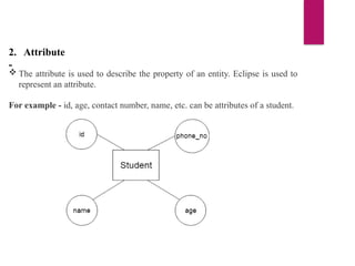
  • 101. Table Borrower Customer name Loan number Saurabh L33 Mehak L49 Ria L98 Table Depositor Customer name Account number Saurabh 1111 Mehak 1113 Suniti 1114 Example – Find the loan number, branch, and amount of loans greater than or equal to 10000 amount. {t| t loan ∈ ∧ t[amount]>=10000}
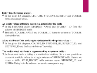
  • 102. Resulting relation - Loan number Branch name Amount L33 ABC 10000 L35 DEF 15000 L98 DEF 65000 Example 2 - Find the loan number for each loan of an amount greater or equal to 10000. {t| s loan(t[loan number] = s[loan number] ∃ ∈ ∧ s[amount]>=10000)}
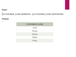
  • 103. Resulting relation - Loan number L33 L35 L98 Example 3 - Find the names of all customers who have a loan and an account at the bank. {t | s borrower( t[customer-name] = s[customer-name]) u depositor( t[customer-name] = u[customer- ∃ ∈ ∧ ∃ ∈ name])} Resulting relation - Customer name Saurabh Mehak