


![are reached, the recursive calls start to return, and their respective nodes in the tree are marked with the returned values.
The traversal continues until the entire tree has been traversed.
Time Complexity Analysis
Recursion trees aid in analyzing the time complexity of recursive algorithms. By examining the structure of the tree, we
can determine the number of recursive calls made and the work done at each level. This analysis helps in understanding
the overall efficiency of the algorithm and identifying any potential inefficiencies or opportunities for optimization.
Introduction
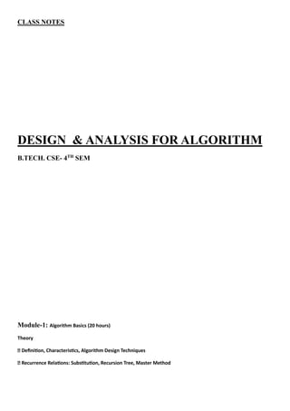
o Think of a program that determines a number's factorial. This function takes a number N as an input and returns
the factorial of N as a result. This function's pseudo-code will resemble,
1. // find factorial of a number
2. factorial(n) {
3. // Base case
4. if n is less than 2: // Factorial of 0, 1 is 1
5. return n
6.
7. // Recursive step
8. return n * factorial(n-1); // Factorial of 5 => 5 * Factorial(4)...
9. }
10.
11. /* How function calls are made,
12.
13. Factorial(5) [ 120 ]
14. |
15. 5 * Factorial(4) ==> 120
16. |
17. 4. * Factorial(3) ==> 24
18. |
19. 3 * Factorial(2) ==> 6
20. |
21. 2 * Factorial(1) ==> 2
22. |
23. 1
24.](https://image.slidesharecdn.com/module-1-classnotesdaa-250327121619-c723076d/85/Disign-and-Analysis-for-algorithm-in-computer-science-and-technology-8-320.jpg)


![How does this work?
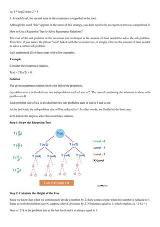
The master method is mainly derived from the recurrence tree method. If we draw the recurrence tree of T(n) =
aT(n/b) + f(n), we can see that the work done at the root is f(n), and work done at all leaves is Θ(nc
) where c is Logba.
And the height of the recurrence tree is Logbn
In the recurrence tree method, we calculate the total work done. If the work done at leaves is polynomially more, then
leaves are the dominant part, and our result becomes the work done at leaves (Case 1). If work done at leaves and root
is asymptotically the same, then our result becomes height multiplied by work done at any level (Case 2). If work done
at the root is asymptotically more, then our result becomes work done at the root (Case 3).
Examples of some standard algorithms whose time complexity can be evaluated using the Master Method
• Merge Sort: T(n) = 2T(n/2) + Θ(n). It falls in case 2 as c is 1 and Logba] is also 1. So the solution is Θ(n Logn)
• Binary Search: T(n) = T(n/2) + Θ(1). It also falls in case 2 as c is 0 and Logba is also 0. So the solution is
Θ(Logn)
Notes:
• It is not necessary that a recurrence of the form T(n) = aT(n/b) + f(n) can be solved using Master Theorem. The
given three cases have some gaps between them. For example, the recurrence T(n) = 2T(n/2) + n/Logn cannot
be solved using master method.
• Case 2 can be extended for f(n) = Θ(nc
Logk
n)
If f(n) = Θ(nc
Logk
n) for some constant k >= 0 and c = Logba, then T(n) = Θ(nc
Logk+1
n)](https://image.slidesharecdn.com/module-1-classnotesdaa-250327121619-c723076d/85/Disign-and-Analysis-for-algorithm-in-computer-science-and-technology-15-320.jpg)
Disign and Analysis for algorithm in computer science and technology
- 1. CLASS NOTES DESIGN & ANALYSIS FOR ALGORITHM B.TECH. CSE- 4TH SEM Module-1: Algorithm Basics (20 hours) Theory Definition, Characteristics, Algorithm Design Techniques Recurrence Relations: Substitution, Recursion Tree, Master Method
- 2. Introduction: What is an algorithm? An Algorithm is a procedure to solve a particular problem in a finite number of steps for a finite-sized input. The algorithms can be classified in various ways. They are: 1. Implementation Method 2. Design Method 3. Design Approaches 4. Other Classifications In this article, the different algorithms in each classification method are discussed. The classification of algorithms is important for several reasons: Organization: Algorithms can be very complex and by classifying them, it becomes easier to organize, understand, and compare different algorithms. Problem Solving: Different problems require different algorithms, and by having a classification, it can help identify the best algorithm for a particular problem. Performance Comparison: By classifying algorithms, it is possible to compare their performance in terms of time and space complexity, making it easier to choose the best algorithm for a particular use case. Reusability: By classifying algorithms, it becomes easier to re-use existing algorithms for similar problems, thereby reducing development time and improving efficiency. Research: Classifying algorithms is essential for research and development in computer science, as it helps to identify new algorithms and improve existing ones. Overall, the classification of algorithms plays a crucial role in computer science and helps to improve the efficiency and effectiveness of solving problems. Classification by Implementation Method: There are primarily three main categories into which an algorithm can be named in this type of classification. They are: 1. Recursion or Iteration: A recursive algorithm is an algorithm which calls itself again and again until a base condition is achieved whereas iterative algorithms use loops and/or data structures like stacks, queues to solve any problem. Every recursive solution can be implemented as an iterative solution and vice versa. Example: The Tower of Hanoi is implemented in a recursive fashion while Stock Span problem is implemented iteratively. 2. Exact or Approximate: Algorithms that are capable of finding an optimal solution for any problem are known as the exact algorithm. For all those problems, where it is not possible to find the most optimized solution, an approximation algorithm is used. Approximate algorithms are the type of algorithms that find the result as an average outcome of sub outcomes to a problem. Example: For NP-Hard Problems, approximation algorithms are used. Sorting algorithms are the exact algorithms. 3. Serial or Parallel or Distributed Algorithms: In serial algorithms, one instruction is executed at a time while parallel algorithms are those in which we divide the problem into subproblems and execute them on different processors. If parallel algorithms are distributed on different machines, then they are known as distributed algorithms.
- 3. Classification by Design Method: There are primarily three main categories into which an algorithm can be named in this type of classification. They are: 1. Greedy Method: In the greedy method, at each step, a decision is made to choose the local optimum, without thinking about the future consequences. Example: Fractional Knapsack, Activity Selection. 2. Divide and Conquer: The Divide and Conquer strategy involves dividing the problem into sub-problem, recursively solving them, and then recombining them for the final answer. Example: Merge sort, Quicksort. 3. Dynamic Programming: The approach of Dynamic programming is similar to divide and conquer. The difference is that whenever we have recursive function calls with the same result, instead of calling them again we try to store the result in a data structure in the form of a table and retrieve the results from the table. Thus, the overall time complexity is reduced. “Dynamic” means we dynamically decide, whether to call a function or retrieve values from the table. Example: 0-1 Knapsack, subset-sum problem. 4. Linear Programming: In Linear Programming, there are inequalities in terms of inputs and maximizing or minimizing some linear functions of inputs. Example: Maximum flow of Directed Graph 5. Reduction(Transform and Conquer): In this method, we solve a difficult problem by transforming it into a known problem for which we have an optimal solution. Basically, the goal is to find a reducing algorithm whose complexity is not dominated by the resulting reduced algorithms. Example: Selection algorithm for finding the median in a list involves first sorting the list and then finding out the middle element in the sorted list. These techniques are also called transform and conquer. 6. Backtracking: This technique is very useful in solving combinatorial problems that have a single unique solution. Where we have to find the correct combination of steps that lead to fulfillment of the task. Such problems have multiple stages and there are multiple options at each stage. This approach is based on exploring each available option at every stage one-by-one. While exploring an option if a point is reached that doesn’t seem to lead to the solution, the program control backtracks one step, and starts exploring the next option. In this way, the program explores all possible course of actions and finds the route that leads to the solution. Example: N-queen problem, maize problem. 7. Branch and Bound: This technique is very useful in solving combinatorial optimization problem that have multiple solutions and we are interested in find the most optimum solution. In this approach, the entire solution space is represented in the form of a state space tree. As the program progresses each state combination is explored, and the previous solution is replaced by new one if it is not the optimal than the current solution. Example: Job sequencing, Travelling salesman problem. Classification by Design Approaches : There are two approaches for designing an algorithm. these approaches include 1. Top-Down Approach : 2. Bottom-up approach • Top-Down Approach: In the top-down approach, a large problem is divided into small sub-problem. and keep repeating the process of decomposing problems until the complex problem is solved. • Bottom-up approach: The bottom-up approach is also known as the reverse of top-down approaches. In approach different, part of a complex program is solved using a programming language and then this is combined into a complete program.
- 4. Top-Down Approach: Breaking down a complex problem into smaller, more manageable sub-problems and solving each sub-problem individually. Designing a system starting from the highest level of abstraction and moving towards the lower levels. Bottom-Up Approach: Building a system by starting with the individual components and gradually integrating them to form a larger system. Solving sub-problems first and then using the solutions to build up to a solution of a larger problem. Note: Both approaches have their own advantages and disadvantages and the choice between them often depends on the specific problem being solved. ############### Recurrence Relation A recurrence is an equation or inequality that describes a function in terms of its values on smaller inputs. To solve a Recurrence Relation means to obtain a function defined on the natural numbers that satisfy the recurrence. Whenever any function makes a recursive call to itself, its time can be computed by a Recurrence Relation. Recurrence Relation is simply a mathematical relation/equation that can give the value of any term in terms of some previous smaller terms. For example, T(n) = T(n-1) + N It is a recurrence relation because the value of the nth term is given in its previous term i.e (n-1)the term. Types of Recurrence Relation: There are different types of recurrence relation that can be possible in the mathematical world. Some of them are- 1. Linear Recurrence Relation: In case of Linear Recurrence Relation every term is dependent linearly on its previous term. Example of Linear Recurrence Relation can be T(n) = T(n-1) + T(n-2) + T(n-3) 2. Divide and Conquer Recurrence Relation: It the type of Recurrence Relation which is obtained from Divide and Conquer Algorithm. Example of such recurrence relation can be T(n) = 3T(n/2) + 9n 3. First Order Recurrence Relation: It is the type of recurrence relation in which every term is dependent on just previous term. Example of this type of recurrence relation can be- T(n) = T(n-1)2 (4) Higher Order Recurrence Relation- It is the type of recurrence relation where one term is not only dependent on just one previous term but on multiple previous terms. If it will be dependent on two previous term then it will be called to be second order. Similarly, for three previous term its will be called to be of third order and so on. Let us see example of an third order Recurrence relation T(n) = 2T(n-1)2 + KT(n-2) + T(n-3)
- 5. Till now we have seen different recurrence relations but how to find time taken by any recursive algorithm. So to calculate time we need to solve the recurrence relation. Now for solving recurrence we have three famous methods- • Substitution Method • Recursive Tree Method • Master Theorem Now in this article we are going to focus on Substitution Method. Substitution Method: Substitution Method is very famous method for solving any recurrences. There are two types of substitution methods- 1. Forward Substitution 2. Backward Substitution 1. Forward Substitution: It is called Forward Substitution because here we substitute recurrence of any term into next terms. It uses following steps to find Time using recurrences- • Pick Recurrence Relation and the given initial Condition • Put the value from previous recurrence into the next recurrence • Observe and Guess the pattern and the time • Prove that the guessed result is correct using mathematical Induction. Now we will use these steps to solve a problem. The problem is- T(n) = T(n-1) + n, n>1 T(n) = 1, n=1 Now we will go step by step- 1. Pick Recurrence and the given initial Condition: T(n)=T(n-1)+n, n>1T(n)=1, n=1 2. Put the value from previous recurrence into the next recurrence: T(1) = 1T(2) = T(1) + 2 = 1 + 2 = 3T(3) = T(2) + 3 = 1 + 2 + 3 = 6T(4)= T(3) + 4 = 1 + 2 + 3 + 4 = 10 3. Observe and Guess the pattern and the time: So guessed pattern will be-T(n) = 1 + 2 + 3 .... + n = (n * (n+1))/2Time Complexity will be O(n2) 4. Prove that the guessed result is correct using mathematical Induction: • Prove T(1) is true: T(1) = 1 * (1+1)/2 = 2/2 = 1 and from definition of recurrence we know T(1) = 1. Hence proved T(1) is true • Assume T(N-1) to be true: Assume T(N-1) = ((N - 1) * (N-1+1))/2 = (N * (N-1))/2 to be true
- 6. • Then prove T(N) will be true:T(N) = T(N-1) + N from recurrence definition Now, T(N-1) = N * (N-1)/2So, T(N) = T(N-1) + N = (N * (N-1))/2 + N = (N * (N-1) + 2N)/2 =N * (N+1)/2And from our guess also T(N)=N(N+1)/2Hence T(N) is true.Therefore our guess was correct and time will be O(N2) 2. Backward Substitution: It is called Backward Substitution because here we substitute recurrence of any term into previous terms. It uses following steps to find Time using recurrences- • Take the main recurrence and try to write recurrences of previous terms • Take just previous recurrence and substitute into main recurrence • Again take one more previous recurrence and substitute into main recurrence • Do this process until you reach to the initial condition • After this substitute the the value from initial condition and get the solution Now we will use these steps to solve a problem. The problem is- T(n) = T(n-1) + n, n>1T(n) = 1, n = 1 Now we will go step by step- 1. Take the main recurrence and try to write recurrences of previous terms: T(n) = T(n-1) + nT(n-1) = T(n-2) + n - 1T(n-2) = T(n-3) + n - 2 2. Take just previous recurrence and substitute into main recurrence put T(n-1) into T(n)So, T(n)=T(n-2)+ n-1 + n 3. Again take one more previous recurrence and substitute into main recurrence put T(n-2) into T(n)So, T(n)=T(n-3)+ n-2 + n-1 + n 4. Do this process until you reach to the initial condition So similarly we can find T(n-3), T(n-4)......and so on and can insert into T(n). Eventually we will get following: T(n)=T(1) + 2 + 3 + 4 +.........+ n-1 + n 5. After this substitute the the value from initial condition and get the solution Put T(1)=1, T(n) = 1 +2 +3 + 4 +..............+ n-1 + n = n(n+1)/2. So Time will be O(N2) Limitations of Substitution method: The Substitution method is a useful technique to solve recurrence relations, but it also has some limitations. Some of the limitations are: • It is not guaranteed that we will find the solution as substitution method is based on guesses. • It doesn't provide guidance on how to make an accurate guess, often relying on intuition or trial and error. • It may only yield a specific or approximate solution rather than the most general or precise one.
- 7. • The substitution method isn't universally applicable to all recurrence relations, especially those with complex or variable forms that do not get simplified using substitution. Recursion Tree Method Recursion is a fundamental concept in computer science and mathematics that allows functions to call themselves, enabling the solution of complex problems through iterative steps. One visual representation commonly used to understand and analyze the execution of recursive functions is a recursion tree. In this article, we will explore the theory behind recursion trees, their structure, and their significance in understanding recursive algorithms. What is a Recursion Tree? A recursion tree is a graphical representation that illustrates the execution flow of a recursive function. It provides a visual breakdown of recursive calls, showcasing the progression of the algorithm as it branches out and eventually reaches a base case. The tree structure helps in analyzing the time complexity and understanding the recursive process involved. Tree Structure Each node in a recursion tree represents a particular recursive call. The initial call is depicted at the top, with subsequent calls branching out beneath it. The tree grows downward, forming a hierarchical structure. The branching factor of each node depends on the number of recursive calls made within the function. Additionally, the depth of the tree corresponds to the number of recursive calls before reaching the base case. Base Case The base case serves as the termination condition for a recursive function. It defines the point at which the recursion stops and the function starts returning values. In a recursion tree, the nodes representing the base case are usually depicted as leaf nodes, as they do not result in further recursive calls. PauseNext Mute Current Time 4:41 / Duration 18:10 Loaded: 31.55% Fullscreen Recursive Calls The child nodes in a recursion tree represent the recursive calls made within the function. Each child node corresponds to a separate recursive call, resulting in the creation of new sub problems. The values or parameters passed to these recursive calls may differ, leading to variations in the sub problems' characteristics. Execution Flow: Traversing a recursion tree provides insights into the execution flow of a recursive function. Starting from the initial call at the root node, we follow the branches to reach subsequent calls until we encounter the base case. As the base cases
- 8. are reached, the recursive calls start to return, and their respective nodes in the tree are marked with the returned values. The traversal continues until the entire tree has been traversed. Time Complexity Analysis Recursion trees aid in analyzing the time complexity of recursive algorithms. By examining the structure of the tree, we can determine the number of recursive calls made and the work done at each level. This analysis helps in understanding the overall efficiency of the algorithm and identifying any potential inefficiencies or opportunities for optimization. Introduction o Think of a program that determines a number's factorial. This function takes a number N as an input and returns the factorial of N as a result. This function's pseudo-code will resemble, 1. // find factorial of a number 2. factorial(n) { 3. // Base case 4. if n is less than 2: // Factorial of 0, 1 is 1 5. return n 6. 7. // Recursive step 8. return n * factorial(n-1); // Factorial of 5 => 5 * Factorial(4)... 9. } 10. 11. /* How function calls are made, 12. 13. Factorial(5) [ 120 ] 14. | 15. 5 * Factorial(4) ==> 120 16. | 17. 4. * Factorial(3) ==> 24 18. | 19. 3 * Factorial(2) ==> 6 20. | 21. 2 * Factorial(1) ==> 2 22. | 23. 1 24.
- 9. 25. */ o Recursion is exemplified by the function that was previously mentioned. We are invoking a function to determine a number's factorial. Then, given a lesser value of the same number, this function calls itself. This continues until we reach the basic case, in which there are no more function calls. o Recursion is a technique for handling complicated issues when the outcome is dependent on the outcomes of smaller instances of the same issue. o If we think about functions, a function is said to be recursive if it keeps calling itself until it reaches the base case. o Any recursive function has two primary components: the base case and the recursive step. We stop going to the recursive phase once we reach the basic case. To prevent endless recursion, base cases must be properly defined and are crucial. The definition of infinite recursion is a recursion that never reaches the base case. If a program never reaches the base case, stack overflow will continue to occur. Recursion Types Generally speaking, there are two different forms of recursion: o Linear Recursion o Tree Recursion o Linear Recursion Linear Recursion o A function that calls itself just once each time it executes is said to be linearly recursive. A nice illustration of linear recursion is the factorial function. The name "linear recursion" refers to the fact that a linearly recursive function takes a linear amount of time to execute. o Take a look at the pseudo-code below: 1. function doSomething(n) { 2. // base case to stop recursion 3. if nis 0: 4. return 5. // here is some instructions 6. // recursive step 7. doSomething(n-1); 8. } o If we look at the function doSomething(n), it accepts a parameter named n and does some calculations before calling the same procedure once more but with lower values. o When the method doSomething() is called with the argument value n, let's say that T(n) represents the total amount of time needed to complete the computation. For this, we can also formulate a recurrence relation, T(n) = T(n-1) + K. K serves as a constant here. Constant K is included because it takes time for the function to allocate or de-allocate memory to a variable or perform a mathematical operation. We use K to define the time since it is so minute and insignificant.
- 10. o This recursive program's time complexity may be simply calculated since, in the worst scenario, the method doSomething() is called n times. Formally speaking, the function's temporal complexity is O(N). Tree Recursion o When you make a recursive call in your recursive case more than once, it is referred to as tree recursion. An effective illustration of Tree recursion is the fibonacci sequence. Tree recursive functions operate in exponential time; they are not linear in their temporal complexity. o Take a look at the pseudo-code below, 1. function doSomething(n) { 2. // base case to stop recursion 3. if n is less than 2: 4. return n; 5. // here is some instructions 6. // recursive step 7. return doSomething(n-1) + doSomething(n-2); 8. } o The only difference between this code and the previous one is that this one makes one more call to the same function with a lower value of n. o Let's put T(n) = T(n-1) + T(n-2) + k as the recurrence relation for this function. K serves as a constant once more. o When more than one call to the same function with smaller values is performed, this sort of recursion is known as tree recursion. The intriguing aspect is now: how time-consuming is this function? o Take a guess based on the recursion tree below for the same function. o It may occur to you that it is challenging to estimate the time complexity by looking directly at a recursive function, particularly when it is a tree recursion. Recursion Tree Method is one of several techniques for calculating the temporal complexity of such functions. Let's examine it in further detail.
- 11. What Is Recursion Tree Method? o Recurrence relations like T(N) = T(N/2) + N or the two we covered earlier in the kinds of recursion section are solved using the recursion tree approach. These recurrence relations often use a divide and conquer strategy to address problems. o It takes time to integrate the answers to the smaller sub problems that are created when a larger problem is broken down into smaller sub problems. o The recurrence relation, for instance, is T(N) = 2 * T(N/2) + O(N) for the Merge sort. The time needed to combine the answers to two sub problems with a combined size of T(N/2) is O(N), which is true at the implementation level as well. o For instance, since the recurrence relation for binary search is T(N) = T(N/2) + 1, we know that each iteration of binary search results in a search space that is cut in half. Once the outcome is determined, we exit the function. The recurrence relation has +1 added because this is a constant time operation. o The recurrence relation T(n) = 2T(n/2) + Kn is one to consider. Kn denotes the amount of time required to combine the answers to n/2-dimensional sub problems. o Let's depict the recursion tree for the aforementioned recurrence relation. We may draw a few conclusions from studying the recursion tree above, including 1. The magnitude of the problem at each level is all that matters for determining the value of a node. The issue size is n at level 0, n/2 at level 1, n/2 at level 2, and so on. 2. In general, we define the height of the tree as equal to log (n), where n is the size of the issue, and the height of this recursion tree is equal to the number of levels in the tree. This is true because, as we just established, the divide-and- conquer strategy is used by recurrence relations to solve problems, and getting from issue size n to problem size 1 simply requires taking log (n) steps. o Consider the value of N = 16, for instance. If we are permitted to divide N by 2 at each step, how many steps are required to get N = 1? Considering that we are dividing by two at each step, the correct answer is 4, which is the value of log(16) base 2. log(16) base 2 log(2^4) base 2 4 * log(2) base 2, since log(a) base a = 1
- 12. so, 4 * log(2) base 2 = 4 3. At each level, the second term in the recurrence is regarded as the root. Although the word "tree" appears in the name of this strategy, you don't need to be an expert on trees to comprehend it. How to Use a Recursion Tree to Solve Recurrence Relations? The cost of the sub problem in the recursion tree technique is the amount of time needed to solve the sub problem. Therefore, if you notice the phrase "cost" linked with the recursion tree, it simply refers to the amount of time needed to solve a certain sub problem. Let's understand all of these steps with a few examples. Example Consider the recurrence relation, T(n) = 2T(n/2) + K Solution The given recurrence relation shows the following properties, A problem size n is divided into two sub-problems each of size n/2. The cost of combining the solutions to these sub- problems is K. Each problem size of n/2 is divided into two sub-problems each of size n/4 and so on. At the last level, the sub-problem size will be reduced to 1. In other words, we finally hit the base case. Let's follow the steps to solve this recurrence relation, Step 1: Draw the Recursion Tree Step 2: Calculate the Height of the Tree Since we know that when we continuously divide a number by 2, there comes a time when this number is reduced to 1. Same as with the problem size N, suppose after K divisions by 2, N becomes equal to 1, which implies, (n / 2^k) = 1 Here n / 2^k is the problem size at the last level and it is always equal to 1.
- 13. Now we can easily calculate the value of k from the above expression by taking log() to both sides. Below is a more clear derivation, n = 2^k o log(n) = log(2^k) o log(n) = k * log(2) o k = log(n) / log(2) o k = log(n) base 2 So the height of the tree is log (n) base 2. Step 3: Calculate the cost at each level o Cost at Level-0 = K, two sub-problems are merged. o Cost at Level-1 = K + K = 2*K, two sub-problems are merged two times. o Cost at Level-2 = K + K + K + K = 4*K, two sub-problems are merged four times. and so on.... Step 4: Calculate the number of nodes at each level Let's first determine the number of nodes in the last level. From the recursion tree, we can deduce this o Level-0 have 1 (2^0) node o Level-1 have 2 (2^1) nodes o Level-2 have 4 (2^2) nodes o Level-3 have 8 (2^3) nodes So the level log(n) should have 2^(log(n)) nodes i.e. n nodes. Step 5: Sum up the cost of all the levels o The total cost can be written as, o Total Cost = Cost of all levels except last level + Cost of last level o Total Cost = Cost for level-0 + Cost for level-1 + Cost for level-2 +.... + Cost for level-log(n) + Cost for last level The cost of the last level is calculated separately because it is the base case and no merging is done at the last level so, the cost to solve a single problem at this level is some constant value. Let's take it as O (1). Let's put the values into the formulae, o T(n) = K + 2*K + 4*K + .... + log(n)` times + `O(1) * n o T(n) = K(1 + 2 + 4 + .... + log(n) times)` + `O(n) o T(n) = K(2^0 + 2^1 + 2^2 + ....+ log(n) times + O(n) If you closely take a look to the above expression, it forms a Geometric progression (a, ar, ar^2, ar^3 ...... infinite time). The sum of GP is given by S(N) = a / (r - 1). Here is the first term and r is the common ratio.
- 14. Recurrence Tree Method: In this method, we draw a recurrence tree and calculate the time taken by every level of the tree. Finally, we sum the work done at all levels. To draw the recurrence tree, we start from the given recurrence and keep drawing till we find a pattern among levels. The pattern is typically arithmetic or geometric series. For example, consider the recurrence relation T(n) = T(n/4) + T(n/2) + cn2 cn2 / T(n/4) T(n/2) If we further break down the expression T(n/4) and T(n/2), we get the following recursion tree. cn2 / c(n2 )/16 c(n2 )/4 / / T(n/16) T(n/8) T(n/8) T(n/4) Breaking down further gives us following cn2 / c(n2 )/16 c(n2 )/4 / / c(n2 )/256 c(n2 )/64 c(n2 )/64 c(n2 )/16 / / / / To know the value of T(n), we need to calculate the sum of tree nodes level by level. If we sum the above tree level by level, we get the following series T(n) = c(n^2 + 5(n^2)/16 + 25(n^2)/256) + …. The above series is a geometrical progression with a ratio of 5/16. To get an upper bound, we can sum the infinite series. We get the sum as (n2 )/(1 – 5/16) which is O(n2 ) Master Method: Master Method is a direct way to get the solution. The master method works only for the following type of recurrences or for recurrences that can be transformed into the following type. T(n) = aT(n/b) + f(n) where a >= 1 and b > 1 There are the following three cases: • If f(n) = O(nc ) where c < Logba then T(n) = Θ(nLogba ) • If f(n) = Θ(nc ) where c = Logba then T(n) = Θ(nc Log n) • If f(n) = Ω(nc ) where c > Logba then T(n) = Θ(f(n))
- 15. How does this work? The master method is mainly derived from the recurrence tree method. If we draw the recurrence tree of T(n) = aT(n/b) + f(n), we can see that the work done at the root is f(n), and work done at all leaves is Θ(nc ) where c is Logba. And the height of the recurrence tree is Logbn In the recurrence tree method, we calculate the total work done. If the work done at leaves is polynomially more, then leaves are the dominant part, and our result becomes the work done at leaves (Case 1). If work done at leaves and root is asymptotically the same, then our result becomes height multiplied by work done at any level (Case 2). If work done at the root is asymptotically more, then our result becomes work done at the root (Case 3). Examples of some standard algorithms whose time complexity can be evaluated using the Master Method • Merge Sort: T(n) = 2T(n/2) + Θ(n). It falls in case 2 as c is 1 and Logba] is also 1. So the solution is Θ(n Logn) • Binary Search: T(n) = T(n/2) + Θ(1). It also falls in case 2 as c is 0 and Logba is also 0. So the solution is Θ(Logn) Notes: • It is not necessary that a recurrence of the form T(n) = aT(n/b) + f(n) can be solved using Master Theorem. The given three cases have some gaps between them. For example, the recurrence T(n) = 2T(n/2) + n/Logn cannot be solved using master method. • Case 2 can be extended for f(n) = Θ(nc Logk n) If f(n) = Θ(nc Logk n) for some constant k >= 0 and c = Logba, then T(n) = Θ(nc Logk+1 n)