Distributed Architecture of Subspace Clustering and Related

1
Jan. 14, 2019
Jay Chang
Subspace Clustering

2
• Feature extraction and clustering at the same time from incomplete tensors data by using
• Subspace clustering and
• Tensor decomposition/completion
• Subspace clustering models (based on spectral clustering):
• SCC (Sparse Subspace Clustering)
• LRR (Low-Rank Representation), BD-LRR (Block Diagonal LRR)…
• LSR (Least Squares Regression)…
• Tensor decomposition/completion algorithms:
• Convex: ADMM
• Non-convex: Bayesian approach (probabilistic model for tensor CP, Tucker or TT)
• Complexity, convergence…
• Applications:
• Face recognition
• Object/action classification
• Face/gait clustering, multi-view clustering
• TIM (Topology Interference Management)
• Challenge competitor:
• PCA (Principal Components Analysis) ? Non-linear space clustering ? …
• TensorFlow regression model ? or SSC + GAN (Generative Adversarial Networks) ? …
Main Goal

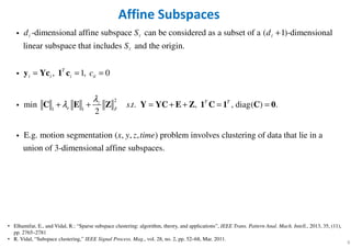
3
Sparse Subspace Clustering
1 1
1
1 1
{ } , linear subspaces, each subspace of dimensions { } , 0 .
noise-free data points { } lie in the union of linear subspaces.
[ ,..., ] [ ,..., ] , is
n n
N D
i i
D N
N n
S n d d D
N n
= =
=
×
< <
∈
≡ = ∈
y
Y y y Y Y Γ Y ℓ
ℓ ℓ ℓ ℓ ℓ
ℓ
i
i ℝ
i ℝ a rank- matrix of the points lie in ,
unknown permutation matrix.
Priori bases of the subspaces and which data points belong to which subspace both unknown.
Subspace Clustering :
N N
d N d S
×
>
∈Γ
ℓ ℓ ℓ ℓ
ℝ
i
i
1 1
finding the number of subspaces, their dimensions,
a basis for each subspace, and the segmentation
Self-expressiveness property
of
:
the data from .
for , 0, [ ,..., ]n
i i i ii i i iNS c c c=∈ = = ≡
Y
y y Yc cℓ ℓi ∪
1
.
There exists a , whose nonzero entries correspond to data points from
the same subspace as . (# nonzero elements dimension of subspace)
In matrix fo
spars
rm : m
e solution
in . .
,
,
i
T
i
s t
=
=
y
C Y
c
YCi 1diag( ) 0, where [ ,..., ] .N N
N
×
= ≡ ∈C C c c ℝ

4
Clustering using Sparse Coefficients
1
Build a weighted graph ( , , )
symmetric non-negative
representing the weights of the edges.
0
, for subspaces .
0
SSC algorithm :
N N
T
n
n
×
=
∈
 
 = + =  
  
W
W similarity matrix
W
W C C W Γ
W
GGGG VVVV EEEEi
ℝ
⋯
i ⋮ ⋱ ⋮
⋯
i
i j
ij ij jiw c c= +

5
Noise and Sparse Outlying Entries
0 0 0 0 0
0
In real-world problems, data are often corrupted by noise and sparse outlying entries.
, sparse outlying entries , noise .
Using the self-expressiveness property
D D
i i i i i i
i c
= + + ∈ ∈
=
y y e z e z
y
i
ℝ ℝ
i 0
0 0 0 0
2
1 1
,
, , .
, diag( ) 0,
where sparse coefficient matrix, sparse outlying matrix, noise matrix.
convex min
2
ij j
j i
i ij j i i i i ij j i i ij jj i j i
j i
z
e F
c c c
λ
λ
≠
≠ ≠
≠
= + + ≡ − ≡ −
= + + =
 + +

  
y
y y e z e e e z z z
Y YC E Z C
C E Z
C E Z
i
i
1
. . , diag( ) ,
/ , / ; , 1; min max , min max .
Use to build a similarity graph and infer the clustering of data using spectral clustering.
T
z z z e e e z e z i j e j
i ij i j i
s t
λ α µ λ α µ α α µ µ
≠ ≠
= + + =
= = > ≡ ≡
Y YC E Z C 0
y y y
Ci

6
Affine Subspaces
2
1 1
-dimensional affine subspace can be considered as a subset of a ( 1)-dimensional
linear subspace that includes and the origin.
, 1, 0
min . .
2
T
i i i ii
z
e F
d S d
S
c
s t
λ
λ
+
= = =
+ + = +
y Yc 1 c
C E Z Y YC
ℓ ℓ ℓ
ℓ
i
i
i , , diag( ) .
E.g. motion segmentation ( , , , ) problem involves clustering of data that lie in a
union of 3-dimensional affine subspaces.
T T
x y z time
+ = =E Z 1 C 1 C 0
i
• Elhamifar, E., and Vidal, R.: “Sparse subspace clustering: algorithm, theory, and applications”, IEEE Trans. Pattern Anal. Mach. Intell., 2013, 35, (11),
pp. 2765–2781
• R. Vidal, “Subspace clustering,” IEEE Signal Process. Mag., vol. 28, no. 2, pp. 52–68, Mar. 2011.

7
Spectral Clustering - Similarity Graphs
Similarity graph ( , ), vertex in graph represents a data point ,
the edge is weighted by 0.
We want to find a partition of the graph such that the edges between different groups
h
i i
ij
G V E v x
w
=
≥
i
i
1
ave very low weights and the edges within a group have high weights.
( , ) be an undirected graph ( ) with vertex set { ,..., },
weighted adjacency matrix, degree matrix defined as
ij ji nG V E w w V v v= = =
W D
i
1
1
,
diagonal matrix.
1, if
A subset of vertices , indicator vector ( ,..., ) .
0, otherwise
For two disjoint sets , , ( , ) .
n
i ij
j
i iT n
A n
i
ij
i A j B
d w
f v A
A V f f
f
A B V W A B w
=
∈ ∈
=
= ∈
⊂ = ∈ 
=
⊂ =


1i ℝ
i
• U. Luxburg, “A tutorial on spectral clustering,” Statistics and Computing, vol. 17, no. 4, pp. 395–416, 2007

8
Spectral Clustering - Similarity Graphs
2
2
-neighborhood graph :
Only include edges with distances , treat as unweighted.
0,
, .
,
-NN ( -Nearest Neighbor) graph :
Connect and if is a k-NN of
ij
ij i j ij
ij
i j j
s
s x x w
s
k k
v v v v
ε
ε
ε
ε ε
<
>
= − = 
≤
i
i
, weighted by similarity .
Directed or undirected.
Mutual -NN graph :
Same as -NN, but only include mutual k-NN.
Fully connected graph :
longer distance lower similarity, Gaussian si
i ij ijw s
k
k
=
i
i
( )2 2
milarity function exp / (2 )i jx x σ− −

9
Unnormalized Graph Laplacians and Their Basic Properties
2
, 1
Unnormalized Laplacian matrix .
is an undirected, weighted graph with weight matrix , where = 0.
1
1. we have ( ) .
2
2. is symmetric and positive semi-
ij ji
n
n T
ij i j
i j
G w w
w f f
=
≥
∀ ∈ = −
= −

W
f f
L
L
W
Lf
D
i
ℝ
1 2
denite.
3. The smallest eigenvalue of is 0, the corresponding eigenvector is the constant one vector .
4. has non-negative, real-valued eigenvalues 0 ... .
Invariance to self-edge
nn λ λ λ= ≤ ≤ ≤
L 1
L
i
1
s : , .
The multiplicity of the eigenvalue 0 of equals the number of connected components ,...,
in the graph. The eigenspace of eigenvalue 0 is spanned by the indicator ve
ii i ii ij ij
k
L d w L w
k A A
= − = −
Li
1
1
2
ctors ,..., of
those components.
, block diagonal form.
kA A
k
 
 
 =
 
 
 
1 1
L
L
L
L
⋱

10
Normalized Graph Laplacians and Their Basic Properties
1/2 1/2 1/2 1/2
1 1
ormalizN .
N
ed symmetry Laplacian matrix
ormalized random walk Laplacian matrix .
sym
rw
− − − −
− −
≡ = −
≡ = −
L D LD I D WD
L D L I D W
i

11
Spectral Clustering Algorithms – Unnormalized
“the first k eigenvectors” corresponding to the k smallest eigenvalues.
= −L D W

12
Spectral Clustering Algorithms – Normalized
1 1
rw
− −
≡ = −L D L I D W

13
Spectral Clustering Algorithms – Normalized
1/2 1/2 1/2 1/2
sym
− − − −
≡ = −L D LD I D WD

14
Graph Cut Point of View
We want to find a partition of the graph such that the edges between different groups
have very low weights and the edges within a group have high weights.
Mincut approach simply consists in ch
i
i 1
1
1
oosing a partition ,..., which minimizes
1
cut( ,..., ) ( , ), where for the complement of .
2
k
k
k i i
i
A A
A A W A A A A
=
≡ 

15
MinCut
• Problem: MinCut favors isolated clusters
• Solution:
• Ratio cuts (RatioCut)
• Normalized cuts (Ncut)

17
RatioCut
• Two measures of size of a subset:
1
1
Given a partition of into sets ,..., define indicator vectors
1/ , if
,..., , and set the matrix .
0, otherwise
min tr( ) . .n k
k
T n kj i j
j j nj j
T T
H
V k A A k
A v A
h h
s t×
×
∈
 ∈
 = = ∈ 

=
h h H
H LH H H
ℝ
i
ℝ
i
nnormalized Lap
.
Correspondin lacian matrixg to u .= −L
I
D Wi

18
NCut
1
1
Given a partition of into sets ,..., define indicator vectors
1/ vol( ), if
,..., , and set the matrix .
0, otherwise
min tr( )n k
k
T j i j n k
j j nj j
T
H
V k A A k
A v A
h h
×
×
∈
 ∈
 = = ∈ 

h h H
H LH
ℝ
i
ℝ
i
1/2 1/2 1/2 1/2
1 1
ormalized symmetry Laplacian matrix
ormalized random walk La
. . .
Corresponding to
N .
placian mN .atrix
T
sym
rw
s t
− − − −
− −
=
≡ = −
≡ = −
H DH I
L D LD I D WD
L D L I D W
i
• Two measures of size of a subset:

19
Low-Rank Representation (LRR)
2
1 1, ,
2,12,1,
SSC : min . . , , diag( ) .
2
LRR (noise-free) : min . . , .
LRR (noise or outliers) : min . . , , where -nor
T Tz
e F
T T
T T
e
s t
s t
s t
λ
λ
λ
∗
∗
+ + = + + = =
= =
+ = + =
C E Z
C
C E
C E Z Y YC E Z 1 C 1 C 0
C Y YC 1 C 1
C E Y YC E 1 C 1
i
i
i ℓ
2
2,1 1 1
m
.
N N
jkk j
E= =
=  E

20
Drawback of SSC/LRR
SSC:
• Disadvantage of SSC is that it is provably correct only in the case of independent or
disjoint subspaces.
LRR:
• Disadvantage of LRR is that it is provably correct only in the case of noiseless data drawn
from independent subspaces.
• Another drawback is that the optimization problem involves O(N2) variables.

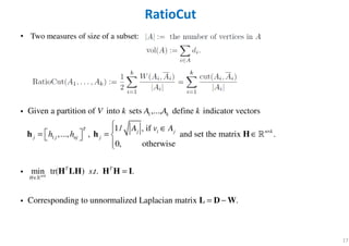
21
Subspace Clustering Model
1 2
1
Given a data set [ , ,..., ] belong to , where is clusters.
k
D N
N i
i
S k×
=
= ∈X x x xi ℝ ∪
• Each data sample xi is represented as a linear combination of other data samples. (Self-
expressiveness property)
( )
self-represe
, ( 1,..., ), 0 for
equivalent to where calle ntation (coefficied matrix.
Affinity matrix define as ,
nt)
Laplacian matrix .
2
i ij j i ij j
j i
N N
T
z S k z Sα αα
≠
×
= ∈ = = ∀ ∉
+
= −
= ∈
=
x x x x
X XZ Z
Z
L
Z
DW W
ℝ
xi

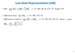
• Sparse Representation (compressive sensing):
• Sparse Subspace Clustering:
23
Sparse Models
0
min
. . .
z
s t y Az=
0
ˆ ˆ 1 1 1
min
. . , where [ ,..., , ,..., ].
i
i i i i Ni i
z
s t x X z X x x x x− += =
0
min
. . , diag( ) 0.s t = =
Z
X XZ Z
1
min
. . , diag( ) 0.s t = =
Z
X XZ Z
R. Vidal and E. Elhamifar, "Sparse subspace clustering," 2009 IEEE Conference on Computer Vision and Pattern Recognition(CVPR), Miami, FL, USA,
2009, pp. 2790-2797.
SIM (Shape Interaction Matrix)

• Matrix Completion (MC):
• Robust PCA:
• Low-Rank Representation (LRR) based clustering:
24
Low-Rank Models
min rank( ) . . ( ) ( ).
, if ( , )
where ( ) project operator
0, otherwise
ij
s t
D i j
π π
π
Ω Ω
Ω
=
∈Ω
= 

A
A D A
D
0,
min rank( ) . . .s tλ+ = +
A E
A E D A E
Filling in missing entries
Denoising
2,0,
min rank( ) . . .s tλ+ = +
Z E
Z E X XZ E Clustering
NP Hard !

25
Low-Rank Models - Convex Formulation
• Matrix Completion (MC):
• Robust PCA:
• Low-Rank Representation (LRR) based clustering:
min . . ( ) ( ).
, if ( , )
where ( ) project operator
0, otherwise
ij
s t
D i j
π π
π
Ω Ω∗
Ω
=
∈Ω
= 

A
A D A
D
1,
min . . .s tλ∗
+ = +
A E
A E D A E
Filling in missing entries
Denoising
2,1,
min . . .s tλ∗
+ = +
Z E
Z E X XZ E Clustering
:,1 2,1 2
,
where ( ), , .i ij j
i i j j
E Eσ∗
= = =  A A E E

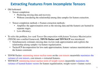
26
Traditional Framework of Sparse Subspace Clustering
Input data Clustering results
Subspace
represent
Spectral clustering
(e.g. Ncut)
Affinity matrix
W
Subspace
coefficient matrix Z
,
1 2 1 2
min ( ) ( ,
[ , ,..., ] , [ , ,..., ] , is error matrix
( , ) denotes loss function, ( ) is regularizer and
is hyperparameter that control
)
s the intensit
. .
y
.
D N N N
N N
L
R L
R
s tλ
λ
× ×
+ =
=
⋅
+
= ∈ ∈
⋅ ⋅
Z E
Z X XZ X XZ
X x Z z z z E
E
x x ℝ ℝ
of the loss penalty.
1
min
. . , diag( ) 0.s t = =
Z
Z
X XZ Z
min
. . , diag( ) 0.s t
∗
= =
Z
Z
X XZ Z
2,1,
min . . .s tλ∗
+ = +
Z E
Z E X XZ E
• General form of subspace clustering representation:
1/2 1/2
RatioCut : arg min tr( ) . . ,
NCut :arg min tr( ) . . .
Spectral clustering :
T T
T T
s t
s t− −
=
=
H
H
H LH H H I
F D LD F F F I
or

27
Database Introduction and How to Deal With
• ORL Database: https://www.cl.cam.ac.uk/research/dtg/attarchive/facedatabase.html
• In orl_faces folder include 40 subfolders (= 40 different people), each subfolder has 10 pictures
(same person) files are in PGM format. The size of each image is 92 x 112 pixels, with 256 grey
levels per pixel.
Downsize to 32 x 32 pixels
and normalized to [0,1].
32
32
400
1024
400
1 2
1
data set [ , ,..., ]
belong to , where is clusters
D N
N
k
i
i
S k
×
=
= ∈X x x x ℝ
∪
×1024 400
=X
or 500
100
∗
=X
PCA
and we hope 40
in this example.
k =

28
Evaluation Metrics
• Normalized Mutual Information (NMI)
• Accuracy (ACC)
• Adjusted Rand Index (ARI)
• F-score
• Precision
• Recall
• Representation Visualization
1 2 1 2
1 1
[ , ,..., ], [ , ,..., ]
( , ) MI( , )
MI( , ) ( , )log , NMI( , )
( ) ( )
entr
( ) ( )
( ) ( )log ( ).opy
r s
r s
i j
k kk
X x x x Y y y y
P i j X Y
X Y P i j X Y
P i P j H X H Y
H P x P x
= =
= =
= =
= −



29
SC Novel Research Approach Including
(1) Design the R(Z) regularization term let the coefficient matrix Z has a good clustering
structure and without losing realistic data hypothesis.
(2) Design L(.) term which robustness to any kind of noise (not just for Gaussian noise).
Bayesian estimation maybe a good way to approach.
(3) Fast and high accuracy algorithm design.
(4) Application exploration.
,
1 2 1 2
min ( ) ( ,
[ , ,..., ] , [ , ,..., ] , is error matrix
( , ) denotes loss function, ( ) is regularizer and
is hyperparameter that control
)
s the intensit
. .
y
.
D N N N
N N
L
R L
R
s tλ
λ
× ×
+ =
=
⋅
+
= ∈ ∈
⋅ ⋅
Z E
Z X XZ X XZ
X x Z z z z E
E
x x ℝ ℝ
of the loss penalty.

30
Drawback of SSC/LRR and Model We Proposed
SSC:
• Disadvantage of SSC is that it is provably correct only in the case of independent or
disjoint subspaces.
LRR:
• Disadvantage of LRR is that it is provably correct only in the case of noiseless data drawn
from independent subspaces.
• Another drawback is that the optimization problem involves O(N2) variables.
Model we proposed:
1 2,1,
2
2,1 2,1 1 1
SSC LRR : min . . , , diag( ) .
where -norm .
T T
N N
jkk j
s t
E
λ∗
= =
+ + + = + + = =
=  
C E
C C E Y YC E Z 1 C 1 C 0
E
i
ℓ

31
Why use L2,1-Norm ?
2
1
2,1
• Illustrating three typical types of errors :
(a) For the small Gaussian noise.
(b) For the random corruptions noise.
(c) For sample-specific corruptions noise and outliers .( )
F
E
E
E
1 2,1,
2
2,1 2,1 1 1
SSC LRR : min . . , , diag( ) .
where -norm .
T T
N N
jkk j
s t
E
λ∗
= =
+ + + = + + = =
=  
C E
C C E Y YC E Z 1 C 1 C 0
E
i
ℓ
G. Liu, Z. Lin, S. Yan, J. Sun, Y. Yu, and Y. Ma, “Robust recovery of subspace structures by low-rank representation,” IEEE Trans. Pattern Anal. Mach.
Intell., vol. 35, no. 1, pp. 171–184, Jan. 2013.

32
Research Interests – YW Peter Hong
Signal Processing & Communication
Mobile Communication
UAV Communications
Machine Learning & Artificial Intelligence
User
Connected UAVs
Beamforming
Broadcasting
physical
connection
Deep Learning based
Communications
Crowdsourcing & IoT
Distributed Learning
Recommender Systems

Centralized Architecture
Centralized
Data Center
34

n data samples
cluster
1
cluster
K
…
n data samples
cluster
1
cluster
K
…
Subspace Clustering (SC)
• Subspace Clustering: Data points from the same
cluster should belong to the same subspace.
 Self Representation Property
n data samples
cluster
1
cluster
K
…
n data samples
cluster
1
cluster
K
…
Different views, but
similar representation
coefficients.
37

Distributed Multi-View SC
Local clustering at node :
Spectral clustering at Center:
Extended Yale-B IXMAS
NMI ACC F1-Score NMI ACC F1-Score
DiMSC 0.580 0.567 0.424 0.655 0.571 0.463
ECMSC 0.780 0.814 0.599 0.656 0.501 0.446
Proposed
DMSC-AE
0.926 0.948 0.892 0.758 0.650 0.540
Spectral
embedding
38

Feature Extraction for Incomplete
Data Via Low-Rank Tensor
Decomposition With Feature
Regularization
40
Q. Shi, Y. M. Cheung, Q. Zhao, H. Lu, "Feature Extraction for Incomplete Data Via Low-Rank Tensor Decomposition With Feature Regularization,"
IEEE Transactions on Neural Networks and Learning Systems, 2018

41
Extracting Features From Incomplete Tensors
• Old fashioned:
• Tensor completion:
• Predicting missing data and recovery.
• Without considering the relationship among data samples for feature extraction.
• Tensor completion methods + Feature extraction methods:
• Amplifies the approximation error as the missing data and the features are learned in
separate stages.
• Low efficiency.
• To solve the problem, low-rank Tensor Decomposition with feature Variance Maximization
(TDVM) into a unified framework, TDVM-Tucker and TDVM-CP was introduced.
• Simultaneously estimates missing data via low-rank approximation and explores the
relationship among samples via feature regularization.
• Tucker/CP decomposition for low-rank approximation, feature variance maximization as
the feature constraint.
• TDVM-Tucker: minimizing tensor nuclear norm on the core tensors meanwhile maximizes the
variance of core tensors, core tensors = extracted features.
• TDVM-CP: minimizing tensor nuclear norm of weight vectors meanwhile maximizes the
variance of learned feature vectors for feature regularization, weight vector = feature vector.

42
Tucker Decomposition
tensor with , , ,I J K P Q R I P J Q K R× × × × × × ×
∈ ∈ ∈ ∈ ∈A B Cℝ ℝ ℝ ℝ ℝX GX GX GX G
core tensor
factor matrix
factor matrix
factor matrix
The factor matrices (which are usually orthogonal) A, B, and C are often referred to as
the principal component in the respective tensor mode.
this will result in a compression of XXXX, with GGGG being the compressed version of XXXX.
is Kronecker product⊗

• Factor matrices:
• Columns of A, B, and C are normalized to length one
• For a general Nth-order tensor
43
Canonical Polyadic (CP) Decomposition
1λ Rλ

44
TDVM-Tucker: Learning Low-dimensional Tensor Features
maximize the variance of learned features
low-rank Tucker approximation, which aims to minimize the reconstruction
error and obtains low-dimensional features.

45
TDVM-CP: Learning Low-dimensional Vector Features

Low-Rank Regularized
Heterogeneous Tensor
Decomposition (LRRHTD) for
Subspace Clustering
46
J. Zhang, X. Li, P. Jing, J. Liu, Y. Su, "Low-rank regularized heterogeneous tensor decomposition for subspace clustering", IEEE Signal Process. Lett.,
vol. 25, no. 3, pp. 333-337, Mar. 2018.

47
tensor with , , ,I J K P Q R I P J Q K R× × × × × × ×
∈ ∈ ∈ ∈ ∈A B Cℝ ℝ ℝ ℝ ℝX GX GX GX G
core tensor
factor matrix
factor matrix
factor matrix
The factor matrices (which are usually orthogonal) A, B, and C are often referred to as
the principal component in the respective tensor mode.
this will result in a compression of XXXX, with GGGG being the compressed version of XXXX.
is Kronecker product⊗

48
• Tucker model can be generalized to N-way tensors
• The concept of n-rank (denoted by rankn(XXXX)): corresponds to the column rank of the n-th
unfolding of the tensor XXXX.
• According to the type of constraints Tucker decomposition approaches can be roughly grouped
into three categories:
• orthogonal tensor decomposition
• non-negative tensor decomposition
• sparse tensor decomposition
• Almost all of the above algorithms decompose tensors based on the isotropy hypothesis (i.e.
orthogonal, non-negative...), meaning that the factor matrices are learned in an equivalent way
for all modes.
• Not suitable for heterogeneous tensor data.
( )rank ( ) rank( )n n= XXXXX

• For all but the last mode, LRRHTD seeks a set of orthogonal projection matrices to map the
original tensor data into a low-dimensional common subspace.
• But for the last mode, a low-rank projection matrix is learned by imposing a nuclear-norm so that
a lowest rank representation that reveals the global structure of samples is obtained for
performing clustering.
• M-th order tensors, N is the total number of samples:
• We concatenate the N tensors to yield a (M + 1)-th order tensor
• The goal of LRRHTD is to find M orthogonal factor matrices for intrinsic
low-dimensional representation and the lowest rank representation using the mapped
low-dimensional tensor as a dictionary, and D < N.
49
Low-Rank Regularized Heterogeneous Tensor
Decomposition (LRRHTD)

• Tucker decomposition of the concatenated tensor XXXX can be estimated in a general form as follows:
where is the core tensor and is the approximation error tensor.
• Cost function:
and
50
arg min

51

Multiview Subspace Clustering
via Tensorial t-Product
Representation
52
M. Yin, J. Gao, S. Xie and Y. Guo, "Multiview Subspace Clustering via Tensorial t-Product Representation,“ IEEE Transactions on Neural Networks
and Learning Systems, pp.1-14, 2018.

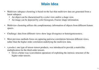
53
• Multiview subspace clustering is based on the fact that multiview data are generated from a
latent subspace.
• An object can be characterized by a color view and/or a shape view.
• An image can be depicted by color histogram, Fourier shape information.
• Multiview clustering utilizes the complementary information of objects from different feature
spaces.
• Challenge: data from different views show large divergence or heterogeneousness.
• Most previous methods focus on capturing pairwise correlations between different views,
rather than the higher order correlation underlying the multiview data.
• t-product, one type of tensor–tensor products, was introduced to provide a matrixlike
multiplication for the third-order tensors.
• Gives a better way (convolution operation) of exploiting the intrinsic structure of the
higher order tensors.
Main Idea

54
Conventional Methods Unfold the Data to Vectors
• ORL Database: https://www.cl.cam.ac.uk/research/dtg/attarchive/facedatabase.html
• In orl_faces folder include 40 subfolders (= 40 different people), each subfolder has 10 pictures
(same person) files are in PGM format. The size of each image is 92 x 112 pixels, with 256 grey
levels per pixel.
Downsize to 32 x 32 pixels
and normalized to [0,1].
32
32
400
1024
400
1 2
1
data set [ , ,..., ]
belong to , where is clusters
D N
N
k
i
i
S k
×
=
= ∈X x x x ℝ
∪
×1024 400
=X
or 500
100
∗
=X
PCA
and we hope 40
in this example.
k =

55
• Conventional methods usually unfold the data to vectors.
• But blindly vectorizing may cause the problem of “curse of dimensionality” and also
damage the second-order structure within data, such as spatial information.
Drawback of Conventional Methods

56
t-Linear Combination for Third-Order Tensor
• Traditional tensor methods (CP, Tucker and HOSVD) are not directly applicable to the third-
order tensors.
• Kilmer et al. presented t-product to define a matrixlike multiplication for third-order tensors.
Called t-Product.
M. E. Kilmer, K. Braman, N. Hao, and R. C. Hoover, “Third-order tensors as operators on matrices: A theoretical and computational framework with
applications in imaging,” SIAM J. Matrix Anal. Appl., vol. 34, no. 1, pp. 148–172, 2013.
matrixm n× 1 tensorm n× ×
3-order tensor is a linear combination of
basis with coefficients .
where is circular convolution operation.∗
AAAA
X BX BX BX B
i
t-linear combination:

57
• A tensor signal represented by a t-linear combination of K tensor dictionary atoms.
t-Linear Combination

58
3-Order Tensor is Built From Different Views

59
Sparse and Low-Rank Representation Using
the t-Linear Combination
• We propose to seek the most sparse and lowest rank representation of multiview data by
employing the self-expressive property.
Most sparse Lowest rank

60
• We propose to seek the most sparse and lowest rank representation of multiview data by
employing the self-expressive property. (continued…)
• fits the representation errors in the 3-order tensor space by using the t-linear combination.
• Different from the previous matricization along certain dimensions, the block circulant
matricization will preserve more spatial correlation within data.
• t-linear combination is a generalization of the standard linear combination.
• is imposed for multiview data encourages consensus representation by forcing all the lowest
rank coefficients close in all views.

61
Overview of the Proposed Framework

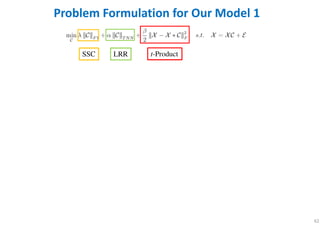
62
Problem Formulation for Our Model 1
SSC LRR t-Product

63
Tensor LRR and
Sparse Coding-Based
Subspace Clustering
Y. Fu, J. Gao, D. Tien, Z. Lin, and X. Hong, “Tensor LRR and sparse coding-based subspace clustering,” IEEE Trans. Neural Netw. Learn. Syst.,
vol. 27, no. 9, pp. 2120–2133, Sep. 2016.
#有德

64
Main Idea
Problems
• Traditional subspace clustering algorithms may be compromised in practical applications:
1. Don’t consider the inherent structure and correlations in the original data.
2. Original high-dimensional features is not effective to filter the noisy/redundant information
in the original feature spaces, and the time complexity grows exponentially with dimensions.
Solutions
1. Finds a lowest rank representation for the input tensor, which can be further used to build an
affinity matrix and then do the spectral clustering.
2. Dictionary learning: finding low-dimensional inherent feature spaces.
• Sparse representation: define holistic sparsity on a whole data representation matrix.
• Sparse coding (SC): finds the sparsest representation of each data vector individually.
• Drawback: SC deteriorates when data are corrupted.
Proposed model
• Input data are represented in their original structural form a tensor.
• Finds the lowest rank representation for each spatial mode of the input tensor.
• Sparse representation with respect to a learned dictionary in the feature mode.
• Spatial spaces + feature spaces to build an affinity matrix for spectral clustering.

65
Dictionary Learning
• Dictionary learning for sparse representation aims at learning a dictionary D, such that each
sample in the data set can be represented as a sparse linear combination of the atoms of D.
• Optimization (e.g. K-SVD):
1. Update zi (SC) by fixing the dictionary D.
2. Update dictionary with a fixed sparse representation.

• Tucker Decomposition:
• Proposed data representation model:
if we let and
• The entries of Z interprets as the similarities between the pairs of all the vectors along the N-mode
of the data tensor X.
• Subspace clustering self-expressiveness: aim to find a linear representation, Z, for all the samples
in terms of all other samples.
66
Tensor Low-Rank Representation on Spatial Modes
core tensor factor matrices
Kronecker product
b = 1 in SSC
b = * in LRR
spatial modes

67
Dictionary Learning for Sparse Representation
on Feature Mode
• We consider a dictionary learning model for sparse representation along the N-mode
(feature mode) of X.
• Feature vectors of each sample can be represented by a few atoms of D.
dictionary to be learned.
mode-N matricization of tensor X(N)
sparse representation on feature spaces.
• Soft reminder TLRR in spatial modes:
feature mode
is the maximum # nonzero elements in
the matrix A.

• Try to combine spatial modes + feature mode.
• Define a transformation of inverse matricization converts a matrix back into an order-N tensor.
•
68
Tensor LRR model
Proposed model
Tensor Spatial Low-Rank Representation
and Feature Sparse Coding
where
feature mode
spatial modes
1 2 1( ... )
where is the dictionary to be learned and
is the sparse representation coefficient matr
feature
ix.
modeN
N
I m
m I I I −
×
×
∈
∈
D
A
ℝ
ℝ
• Finally
proposed
learning model
where R is a given sparsity.

• Finally proposed learning model
• Aims:
• Find the lowest rank representations along all the spatial modes.
• Learn a dictionary with its sparse representation over the samples on the feature mode.
At the same time.
69
Tensor LRR model
Proposed model
b = 1 in SSC
b = * in LRR
spatial modes
feature mode

70
Problem Formulation for Our Model 2
SC LRR Tucker

71
Compare Two Our Models
SSC LRR t-Product
SC LRR Tucker
2,1or robust noise -normℓ

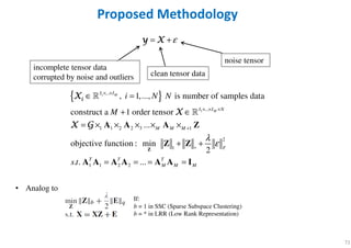
72
ε= +y Xy Xy Xy X
Proposed Methodology
incomplete tensor data
corrupted by noise and outliers clean tensor data
noise tensor
{ }1
1
...
...
1 1 2 2 3 1
2
1
1 1 2 2
, 1,..., is number of samples data
construct a 1 order tensor
...
objective function : min
2
. . ...
M
M
I I
I I N
M M M
F
T T T
M M M
i N N
M
s t
λ
ε
× ×
× × ×
+
∗
∈ =
+ ∈
= × × × × ×
+ +
= = = =
Z
A A A Z
Z Z
A A A A A A I
iiiiXXXX
XXXX
X GX GX GX G
ℝ
ℝ
If:
b = 1 in SSC (Sparse Subspace Clustering)
b = * in LRR (Low Rank Representation)
• Analog to

73
Bayesian Tensor Factorization Probabilistic Model
{ }1
1
...
...
1 1 2 2 3 1
2
1
1 1 2 2
, 1,..., is number of samples data
construct a 1 order tensor
...
objective function : min
2
. . ...
M
M
I I
I I N
M M M
F
T T T
M M M
i N N
M
s t
ε
λ
ε
× ×
× × ×
+
∗
∈ =
+ ∈
= +
= × × × × ×
+ +
= = = =
Z
A A A Z
Z Z
A A A A A A I
iiiiXXXX
XXXX
y Xy Xy Xy X
X GX GX GX G
ℝ
ℝ
Using MAP estimation
max log-joint distribution
Predictive distribution over missing entries
Z
Try to add a
prior on Z
base on SSC
and LRR.

74
Model Learning via Bayesian Inference
• Because integrate over all latent variables as well as hyperparameters is intractable. So
we use variational Bayesian (VB) framework.
• Based on mean-field approximation
We seek a distribution ( ) to approximate the true posterior distribution ( | )
by min KL divergence.
q q ΩΘ Θ yyyyi

75
PARAFAC-based Multilinear
Subspace Clustering
for Tensor data
P. A. Traganitis and G. B. Giannakis, “PARAFAC-based multilinear subspace clustering for tensor data,” in Proc. IEEE Global Conf. Signal Inf. Process.,
Washington, DC, USA, 2016, pp. 1280–1284.

76
Main Idea
• Subspace clustering
• K
aim to find
• When data are high-dimensional both LRR and SSC have high computation complexity.
,
columns form a basis of ,
is low-dimensional representation of in ,
is the "centroid" or intercept of ,
is noise vector,
cluster assignment vector for ,
[ ] de
k
k
D d
k k
d
k n n k
D
k k
D
n
n n
n k
S
S
S
×
∈
∈
∈
∈
U
y x
m
v
π x
π
ℝ
ℝ
ℝ
ℝ
notes the th entry of .nk π
hard clustering
soft/probabilistic clustering

77
• This work aims to extend the union of subspaces model, used by the SC algorithms, to a union
of multilinear subspaces.
• This given data can be reshaped in a tensor format.
• Data in the same cluster share the factor matrices Bk, Ak, and differ only in the factor matrix Ck.
Implies that each cluster k can be represented by a tensor Xk.
Main Idea

79
6 8 1
7 4 9
3 5 2
1 2 6
7 7 3
8 2 1
8 8 1
4 1 9
1 8 3
9 8 8
1 1 4
7 4 9
(user-user)
(celebrity-celebrity)
(movie-movie)
correlation matrix
correlation matrix
correlation
matrix

81
Five Pillars Of The Mamba Mentality:
1. Be Passionate.
2. Be Obsessive.
3. Be Relentless.
4. Be Resilient.
5. Be Fearless.
“Obsessiveness is having the attention to detail for the action you are performing at the time
you’re performing it.”
“Success is the ability to use your passion to help someone else discover their passion.”
https://www.youtube.com/watch?v=NLElzEJPceA

82https://www.ted.com/talks/linda_hill_how_to_manage_for_collective_creativity

83
Thank you for your attention

Distributed Architecture of Subspace Clustering and Related

Recommended

More Related Content

What's hot (20)

Similar to Distributed Architecture of Subspace Clustering and Related (20)

More from Pei-Che Chang (20)

Recently uploaded (20)

Distributed Architecture of Subspace Clustering and Related