Dynamic Programming for 4th sem cse students

Dynamic Programming
Dynamic Programming is a general algorithm design technique
for solving problems defined by recurrences with overlapping
subproblems
• Invented by American mathematician Richard Bellman in the
1950s to solve optimization problems and later assimilated by CS
• “Programming” here means “planning”
• Main idea:
- set up a recurrence relating a solution to a larger instance
to solutions of some smaller instances
- solve smaller instances once
- record solutions in a table
- extract solution to the initial instance from that table

Example 1: Fibonacci numbers
• Recall definition of Fibonacci numbers:
F(n) = F(n-1) + F(n-2)
F(0) = 0
F(1) = 1
• Computing the nth Fibonacci number recursively (top-down):
F(n)
F(n-1) + F(n-2)
F(n-2) + F(n-3) F(n-3) + F(n-4)
...

Example 1: Fibonacci numbers (cont.)
Computing the nth Fibonacci number using bottom-up iteration
and recording results:
F(0) = 0
F(1) = 1
F(2) = 1+0 = 1
…
F(n-2) =
F(n-1) =
F(n) = F(n-1) + F(n-2)
0 1 1 . . . F(n-2) F(n-1) F(n)

DP Steps
F(n) = max{cn + F(n-2), F(n-1)} for n > 1,
F(0) = 0, F(1)=c₁
1. Recursive math function describing maximum
2. Recursive function solving problem, top down (too slow)
3. Iterative solution, bottom up
4. Add information to find how to get maximum
5. Work backward to find maximum

Other examples of DP algorithms
• Computing a binomial coefficient
•General case of the change making problem
• Some difficult discrete optimization problems:
- knapsack
- traveling salesman
• Constructing an optimal binary search tree
• Warshall’s algorithm for transitive closure
•Floyd’s algorithm for all-pairs shortest paths

Dynamic Programming for 4th sem cse students

Warshall’s Algorithm: Transitive Closure
• Computes the transitive closure of a relation
• Alternatively: existence of all nontrivial paths in a digraph
• Example of transitive closure:
3
4
2
1
0 0 1 0
1 0 0 1
0 0 0 0
0 1 0 0
0 0 1 0
1 1 1 1
0 0 0 0
1 1 1 1
3
4
2
1

Warshall’s Algorithm (recurrence)
On the k-th iteration, the algorithm determines for every pair of
vertices i, j if a path exists from i and j with just vertices 1,…,k
allowed as intermediate
R(k-1)[i,j] (path using just 1 ,…,k-1)
R(k)[i,j] = or
R(k-1)[i,k] and R(k-1)[k,j] (path from i to k
and from k to i
using just 1 ,…,k-1)
i
j
k
{

Warshall’s Algorithm (matrix generation)
Recurrence relating elements R(k) to elements of R(k-1) is:
R(k)[i,j] = R(k-1)[i,j] or (R(k-1)[i,k] and R(k-1)[k,j])
It implies the following rules for generating R(k) from R(k-1):
Rule 1 If an element in row i and column j is 1 in R(k-1),
it remains 1 in R(k)
Rule 2 If an element in row i and column j is 0 in R(k-1),
it has to be changed to 1 in R(k) if and only if
the element in its row i and column k and the element
in its column j and row k are both 1’s in R(k-1)

Warshall’s Algorithm
Constructs transitive closure T as the last matrix in the sequence
of n-by-n matrices R(0), … , R(k), … , R(n) where
R(k)[i,j] = 1 iff there is nontrivial path from i to j with only first k
vertices allowed as intermediate
Note that R(0) = A (adjacency matrix), R(n) = T (transitive closure)
3
4
2
1
3
4
2
1
3
4
2
1
3
4
2
1
R(0)
0 0 1 0
1 0 0 1
0 0 0 0
0 1 0 0
R(1)
0 0 1 0
1 0 1 1
0 0 0 0
0 1 0 0
R(2)
0 0 1 0
1 0 1 1
0 0 0 0
1 1 1 1
R(3)
0 0 1 0
1 0 1 1
0 0 0 0
1 1 1 1
R(4)
0 0 1 0
1 1 1 1
0 0 0 0
1 1 1 1
3
4
2
1

Warshall’s Algorithm (example)
3
4
2
1 0 0 1 0
1 0 0 1
0 0 0 0
0 1 0 0
R(0) =
0 0 1 0
1 0 1 1
0 0 0 0
0 1 0 0
R(1) =
0 0 1 0
1 0 1 1
0 0 0 0
1 1 1 1
R(2) =
0 0 1 0
1 0 1 1
0 0 0 0
1 1 1 1
R(3) =
0 0 1 0
1 1 1 1
0 0 0 0
1 1 1 1
R(4) =

Warshall’s Algorithm (pseudocode and analysis)
Time efficiency: Θ(n3)
Space efficiency: Matrices can be written over their predecessors

Floyd’s Algorithm: All pairs shortest paths
Problem: In a weighted (di)graph, find shortest paths between
every pair of vertices
Same idea: construct solution through series of matrices D(0), …,
D (n) using increasing subsets of the vertices allowed
as intermediate
Example: 3
4
2
1
4
1
6
1
5
3

Floyd’s Algorithm (matrix generation)
On the k-th iteration, the algorithm determines shortest paths
between every pair of vertices i, j that use only vertices among
1,…,k as intermediate
D(k)[i,j] = min {D(k-1)[i,j], D(k-1)[i,k] + D(k-1)[k,j]}
i
j
k
D(k-1)[i,j]
D(k-1)[i,k]
D(k-1)[k,j]

Floyd’s Algorithm (example)
0 ∞ 3 ∞
2 0 ∞ ∞
∞ 7 0 1
6 ∞ ∞ 0
D(0) =
0 ∞ 3 ∞
2 0 5 ∞
∞ 7 0 1
6 ∞ 9 0
D(1) =
0 ∞ 3 ∞
2 0 5 ∞
9 7 0 1
6 ∞ 9 0
D(2) =
0 10 3 4
2 0 5 6
9 7 0 1
6 16 9 0
D(3) =
0 10 3 4
2 0 5 6
7 7 0 1
6 16 9 0
D(4) =
3
1
3
2
6 7
4
1 2
D(3): 3 to 1 not allowing 4=9. D(4): 3 to 1 with allowing 4=7

Floyd’s Algorithm (pseudocode and analysis)
Time efficiency: Θ(n3)
Space efficiency: Matrices can be written over their predecessors
Note: Shortest paths themselves can be found, too (Problem 10)

Knapsack Problem by DP
Given n items of
integer weights: w1 w2 … wn
values: v1 v2 … vn
a knapsack of integer capacity W
find most valuable subset of the items that fit into the knapsack
Consider instance defined by first i items and capacity j (j  W).
Let V[i,j] be optimal value of such instance. Then
max {V[i-1,j], vi + V[i-1,j- wi]} if j- wi  0
V[i,j] =
V[i-1,j] if j- wi < 0
Initial conditions: V[0,j] = 0 and V[i,0] = 0

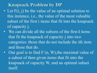
• Let F(i, j) be the value of an optimal solution to
this instance, i.e., the value of the most valuable
subset of the first i items that fit into the knapsack
of capacity j.
• We can divide all the subsets of the first i items
that fit the knapsack of capacity j into two
categories: those that do not include the ith item
and those that do.
• Our goal is to find F (n, W),the maximal value of
a subset of then given items that fit into the
knapsack of capacity W, and an optimal subset
itself.
Knapsack Problem by DP

Table for solving the knapsack problem by dynamic
programming
Recurrence relation for the knapsack problem by dynamic
programming

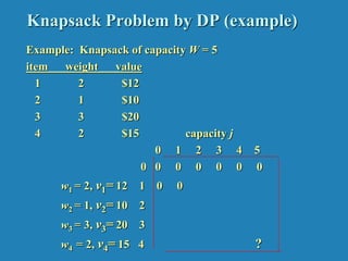
Knapsack Problem by DP (example)
Example: Knapsack of capacity W = 5
item weight value
1 2 $12
2 1 $10
3 3 $20
4 2 $15 capacity j
0 1 2 3 4 5
0 0 0 0 0 0 0
w1 = 2, v1= 12 1 0 0
w2 = 1, v2= 10 2
w3 = 3, v3= 20 3
w4 = 2, v4= 15 4 ?

Example: Knapsack of capacity W = 5
item weight value
1 2 $12
2 1 $10
3 3 $20
4 2 $15 capacity j
0 1 2 3 4 5
0 0 0 0 0 0 0
w1 = 2, v1= 12 1 0 0 12 12 12 12
w2 = 1, v2= 10 2 0 10 12 22 22 22
w3 = 3, v3= 20 3 0 10 12 22 30 32
w4 = 2, v4= 15 4 0 10 15 25 30 37

V[i,j]= max(v[i-1, j] , vi + v[i-1, j-wi] if j-wi >=0
v[i-1, j] if j-wi < 0
v[1,1] = 1-2= -1 j-wi<0 = v[0,1]=0
v[1,2]=max(0,12+0)=12
v[2,3]=max(12,10+12)=22
v[3,5]=max(22,20+12)=32
capacity j
0 1 2 3 4 5
0 0 0 0 0 0 0
w1 = 2, v1= 12 1 0 0 12 12 12 12
w2 = 1, v2= 10 2 0 10 12 22 22 22
w3 = 3, v3= 20 3 0 10 12 22 30 32
w4 = 2, v = 15 4 0 10 15 25 30 37

V[i,j]= max(v[i-1, j] , vi + v[i-1, j-wi] if j-wi >=0
v[i-1, j] if j-wi < 0
v[1,1] = 1-2= -1 j-wi<0 = v[0,1]=0
v[1,2]=max(0,12+0)=12 v[4,5]= max(32, 15+22) =37
v[2,3]=max(12,10+12)=22
v[3,5]=max(22,20+12)=32
capacity j
0 1 2 3 4 5
0 0 0 0 0 0 0
w1 = 2, v1= 12 1 0 0 12 12 12 12
w2 = 1, v2= 10 2 0 10 12 22 22 22
w3 = 3, v3= 20 3 0 10 12 22 30 32
w4 = 2, v4= 15 4 0 10 15 25 30 37

To know which objects are placed, v[objects, capacity]
If v[4,5] != v[3,5], 4th object is placed else it is not placed
37 != 32 therefore 4th object is placed
Decrease the capacity by the weight of the object
v[3, 5-2]= v[3,3] = v[2,3] , object 3 not placed
v[2,3]!= v[1,3]] 2nd object is placed
v[1, 3-1] = v[1,2] != v[0,2], 1st object is placed
capacity j
0 1 2 3 4 5
0 0 0 0 0 0 0
w1 = 2, v1= 12 1 0 0 12 12 12 12
w2 = 1, v2= 10 2 0 10 12 22 22 22
w3 = 3, v3= 20 3 0 10 12 22 30 32
w4 = 2, v4= 15 4 0 10 15 25 30 37

Optimal Binary Search Trees
Problem: Given n keys a1 < …< an and probabilities p1 ≤ … ≤ pn
searching for them, find a BST with a minimum
average number of comparisons in successful search.
Since total number of BSTs with n nodes is given by
C(2n,n)/(n+1), which grows exponentially, brute force is hopeless.
Example: What is an optimal BST for keys A, B, C, and D with
search probabilities 0.1, 0.2, 0.4, and 0.3, respectively?
What smaller problems could we use?
Let’s first look at an example.

Example: key A B C D
probability 0.1 0.2 0.4 0.3
Expected number of comparisons?
optimal BST
B
A
C
D

Expected number of comparisons for optimal BST:
1*0.4 + 2*(0.2+0.3) + 3*(0.1) = 0.4+1.0+0.3=1.7
Non-optimal BST – Swap A and B:
1*0.4 + 2*(0.1+0.3) + 3*(0.2) = 0.4+0.8+0.6=1.8
optimal BST
B
A
C
D

1*0.4 + 2*(0.2+0.3) + 3*(0.1) = 0.4+1.0+0.3=1.7
Can factor out cost of visiting each node once:
1*0.4 + 2*(0.2+0.3) + 3*(0.1) = 0*.4+1*.5+2*.1 + 1*(.4+.5+.1)
Moving subtree up or down changes total by weight of subtree
- BA at level 1/2 has cost 1*.2 + 2*.1 = .4 =
- BA at level 2/3 has cost 2*.2 + 3*.1 = .7 = .4 + (.2 + .1)
- BA at level 3/4 has cost ???
optimal BST
B
A
C
D

1*0.4 + 2*(0.2+0.3) + 3*(0.1) = 0.4+1.0+0.3=1.7
Can factor out cost of visiting each node once:
1*0.4 + 2*(0.2+0.3) + 3*(0.1) = 0*.4+1*.5+2*.1 + 1*(.4+.5+.1)
Moving subtree up or down changes total by weight of subtree
- BA at level 1/2 has cost 1*.2 + 2*.1 = 0.4 =
- BA at level 2/3 has cost 2*.2 + 3*.1 = 0.7 = .4 + (.2 + .1)
- BA at level 3/4 has cost 3*.2 + 4*.1 = 1.0 = .4 + (.2 + .1)
optimal BST
B
A
C
D

What if we let each element be the root?
What is needed then?

DP for Optimal BST Problem
Let T[i,j] be optimal BST for keys ai < …< aj , C[i,j] be minimum
average number of comparisons made in T[i,j], for 1 ≤ i ≤ j ≤ n.
Consider optimal BST among all BSTs with some ak (i ≤ k ≤ j )
as their root; T[i,j] is the best among them.
a
Optimal
BST for
a , ..., a
Optimal
BST for
a , ..., a
i
k
k-1 k+1 j
C[i,j] =
min {pk · 1 +
∑ ps · (level as in T[i,k-1] +1) +
∑ ps · (level as in T[k+1,j] +1)}
i ≤ k ≤ j
s = i
k-1
s =k+1
j
Min Num Comparisons
Best Tree

DP for Optimal BST Problem (cont.)
After simplifications, we obtain the recurrence for C[i,j]:
C[i,j] = min {C[i,k-1] + C[k+1,j]} + ∑ ps for 1 ≤ i ≤ j ≤ n
C[i,i] = pi for 1 ≤ i ≤ j ≤ n
What table elements are involved?
s = i
j
i ≤ k ≤ j

goal
0
0
C[i,j]
0
1
n+1
0 1 n
p 1
p2
n
p
i
j
DP for Optimal BST Problem (cont.)
After simplifications, we obtain the recurrence for C[i,j]:
C[i,j] = min {C[i,k-1] + C[k+1,j]} + ∑ ps for 1 ≤ i ≤ j ≤ n
C[i,i] = pi for 1 ≤ i ≤ j ≤ n
s = i
j
i ≤ k ≤ j

The left table is filled using the recurrence
C[i,j] = min {C[i,k-1] + C[k+1,j]} + ∑ ps , C[i,i] = pi
The right saves the tree roots, which are the k’s that give the minima
0 1 2 3 4
1 0 .1 .4 1.1 1.7
2 0 .2 .8 1.4
3 0 .4 1.0
4 0 .3
5 0
0 1 2 3 4
1 1 2 3 3
2 2 3 3
3 3 3
4 4
5
i ≤ k ≤ j s = i
j
optimal BST
B
A
C
D
i
j i
j
Tables filled diagonal by diagonal (remember what C[i,j] is).

Analysis DP for Optimal BST Problem
Time efficiency: Θ(n3) but can be reduced to Θ(n2) by taking
advantage of monotonicity of entries in the
root table, i.e., R[i,j] is always in the range
between R[i,j-1] and R[i+1,j]
Space efficiency: Θ(n2)
Method can be expanded to include unsuccessful searches

Dynamic Programming for 4th sem cse students

More Related Content

Similar to Dynamic Programming for 4th sem cse students (20)

Recently uploaded (20)

Dynamic Programming for 4th sem cse students