E views 6 users guide i
1 like705 views

This document is the user guide for EViews 6. It covers copyright information and the disclaimer, then provides a table of contents outlining the guide's chapters which cover topics like the basics of EViews, workfiles, objects, data handling, and more advanced features. The guide is intended to help users learn how to use EViews for tasks like importing data, estimating models, testing hypotheses, and forecasting. It provides instructions and explanations throughout.


![Numeric Expressions—127
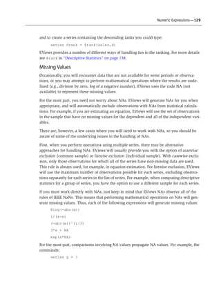
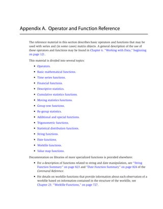
You can take higher order differences by specifying the difference order. For example, the
expressions:
d(income,4)
dlog(income,4)
represent the fourth-order differences of INCOME and log(INCOME).
If you wish to take seasonal differences, you should specify both the ordinary, and a sea-
sonal difference term:
d(income,1,4)
dlog(income,1,4)
These commands produce first order differences with a seasonal difference at lag 4. If you
want only the seasonal difference, specify the ordinary difference term to be 0:
d(income,0,4)
dlog(income,0,4)
Other time series functions provided by EViews include a number of percentage change type
functions. The simplest of these, @pc calculates a simple one-period percentage change in a
series. For example typing:
@pca(income)
calculates the annual percentage change in INCOME.
Two special types of time series functions, moving functions and cumulative functions are
also available in EViews, and are described below.
Mathematical details of lags, leads, differences and percentage change functions are pro-
vided in Appendix A. “Operator and Function Reference,” on page 733.
Cumulative and Moving Statistic Functions
Cumulative and moving statistic functions provide information over a range, or “window” of
observations. The cumulative functions come in two types, those that move forwards and
those that move backwards. The forwards functions, which take the form @cum[stat], have
a window that starts at the start of the workfile (or if a sample is given in the function, from
the start of the sample) up until the current observation.
The backwards functions, which take the form @cumb[stat], start at the end of the workfile,
or sample, and move backwards until the current observation.
Note for both type of cumulative function the length of the window is different for each
observation. The cumulative functions may be thought of as perform “running total” type
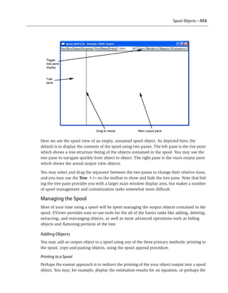
calculations. Missing values are not propagated in the cumulative functions, i.e., observa-](https://image.slidesharecdn.com/eviews6usersguidei-150511081027-lva1-app6892/85/E-views-6-users-guide-i-141-320.jpg)
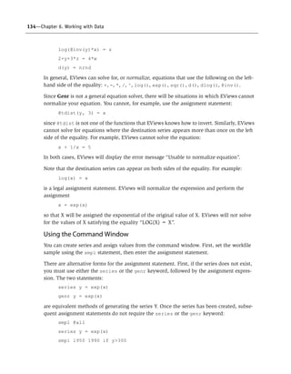
![128—Chapter 6. Working with Data
tions with a value equal to NA are simply skipped. More information on Missing Values is
given below in “Missing Values” on page 129.
The moving statistic functions have a shorter, user specified, window length. They provide
information on the n observations up to, and including, the current observation, where n is
chosen by the user.
The moving functions come in two types, those that propagate missing values and those
that do not. For the functions that do propagate missing values, which take the form
@mov[stat], if any of the observations within the window contain an NA the function will
return NA. The functions that do not propagate, which take the form @m[stat], will simply
skip any NA observations. For more information on missing values see “Missing Values” on
page 129.
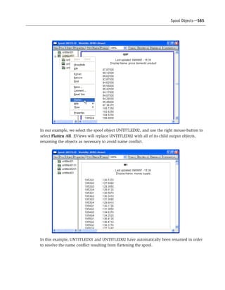
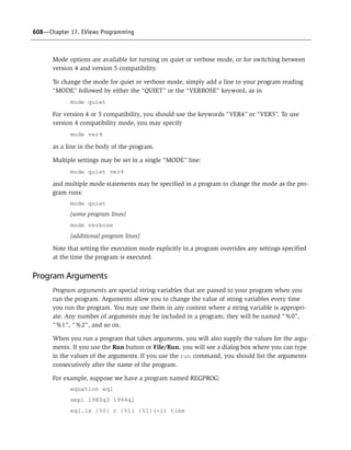
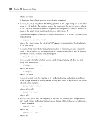
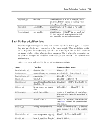
As an example, you could find out the maximum value of INCOME from the start of the
workfile to each observation by typing:
show @cummax(income)
If the first, say, four observations of INCOME are 100, 120, 110, 140 then this command will
show a series as 100, 120, 120, 140 as the first four observations.
If you wanted to know at each observation the average of the previous 3 years (including the
current year) SALES figures you could type:
show @movav(sales,3)
Note this is equal to:
show (sales + sales(-1) + sales(-2))/3
Note that the lag or lead operators can be used inside a moving statistic function to allow
you to control the exact start and end point of your window. For example if you wanted to
know, at each observation, the sum of SALES from three years ago, two years ago and last
year (i.e. the sum of SALES(-1), SALES(-2) and SALES(-3) ) you could type:
show @movsum(sales(-1),3)
Further details and a complete list of cumulative functions can be found in “Cumulative Sta-
tistic Functions” on page 741, and for moving functions in “Moving Statistic Functions” on
page 743.
Ranking Series
EViews has an @rank function which will generate a series based upon the ranking of
another series. Ranking can be either ascending or descending depending upon whether “a”
or “d” is used as an option in the function. For example to create series, ARANK, which con-
tains the ascending ranks of the observations in the series SALES you could type:
series arank = @rank(sales,a)](https://image.slidesharecdn.com/eviews6usersguidei-150511081027-lva1-app6892/85/E-views-6-users-guide-i-142-320.jpg)


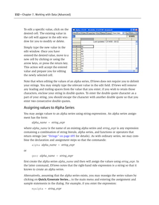


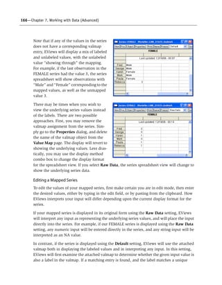
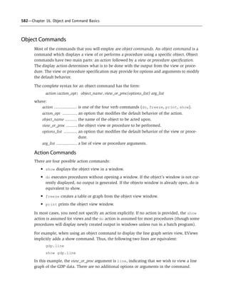
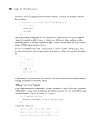
![Date Series—157
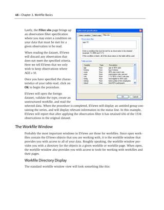
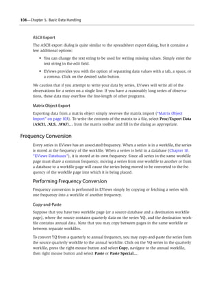
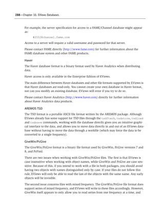
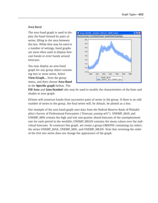
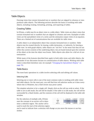
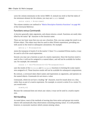
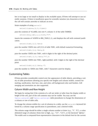
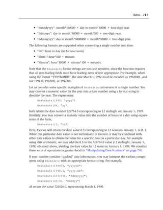
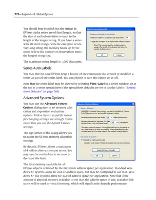
For example, the following series
QDATES in our quarterly workfile is
a numeric series containing valid
date values for the start of each
quarter. The numeric values of
QDATES depicted here show the
number of days since 1 January
A.D. 1.
Obviously, this is not the way that
most people will wish to view their
date series. Accordingly, EViews
provides considerable control over
the display of the date values in
your series. To change the display, click on the Properties button in the series toolbar, or
select View/Properties... from the main menu.
EViews will display a dialog prompting you to change the display properties of the series.
While you may change a variety of display settings such as the column width, justification,
and indentation, here, for the moment, we are more interested in setting the properties of
the Numeric Display.
For a date series, there are four settings of interest in the Numeric Display combo box
(Period, Day, Day-Time, and Time), with each corresponding to specific information that
we wish to display in the series spreadsheet. For example, the Day selection allows you to
display date information up to the day in various formats; with year, month, and day all
included in the representation.
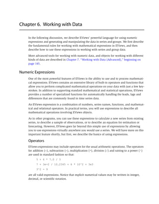
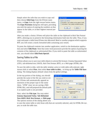
Let us consider our quarterly workfile
example. Here we have selected Period and
chosen a specific Date format entry
(“YYYY[Q]Q”), which tells EViews that
you wish to display the year, followed by
the “Q” separator, and then the quarter
number. Note also that when Period is
selected, there is a Current Workfile set-
ting in the Date format combo box which
tells EViews to use the current workfile dis-
play settings.
The two checkboxes below the Date for-
mat combo box may be used to modify the
selected date format. If you select Two digit year, EViews will only display the last two-dig-](https://image.slidesharecdn.com/eviews6usersguidei-150511081027-lva1-app6892/85/E-views-6-users-guide-i-171-320.jpg)
![158—Chapter 7. Working with Data (Advanced)
its of the year (if the selected format is “YYYY[Q]Q”, the actual format used will be
“YY[Q]Q”); if you select Day/month order, days will precede months in whichever format is
selected (if you select “mm/dd/YYYY” as the format for a day display, EViews will use “dd/
mm/YYYY”).
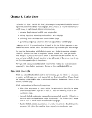
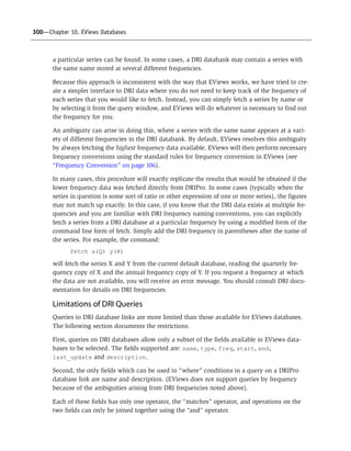
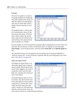
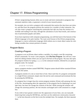
Applying this format to the QDATES series, the display changes to show the data in the new
format:
If instead we select the Day display, and choose the “YYYY-MM-DD” format, the QDATES
spreadsheet will show:
There is one essential fact to remember about the QDATES series. Despite the fact that we
have changed the display to show a text representation of the date, QDATES still contains
the underlying numeric date values. This is in contrast to using an alpha series to hold a text
representation of the date.](https://image.slidesharecdn.com/eviews6usersguidei-150511081027-lva1-app6892/85/E-views-6-users-guide-i-172-320.jpg)


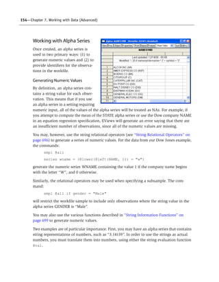
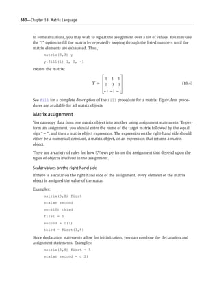
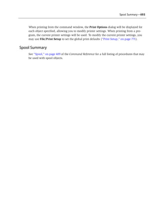
![Value Maps—161
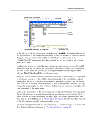
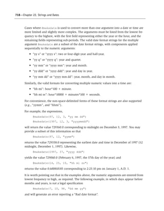
Defining a Valmap
To create a valmap object, select
Object/New Object.../ValMap from
the main menu and optionally enter
an object name, or enter the keyword
“VALMAP” in the command line, fol-
lowed by an optional name. EViews
will open a valmap object.
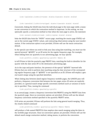
You will enter your new mappings
below the double line by typing or by
copy-and-pasting. In the Value col-
umn, you should enter the values for which you wish to provide labels; in the Label col-
umn, you will enter the corresponding text label. Here, we define a valmap named
FEMALEMAP in which the value 0 is mapped to the string “Male”, and the value 1 is
mapped to the string “Female”.
The two special entries above the double line should be used to define mappings for blank
strings and numeric missing values. The default mapping is to represent blank strings as
themselves, and to represent numeric missing values with the text “NA”. You may change
these defaults by entering the appropriate text in the Label column. For example, to change
the representation of missing numeric values to, say, a period, simply type the “.” character
in the appropriate cell.
We caution that when working with maps, EViews will look for exact equality between the
value in a series and the value in the valmap. Such an equality comparison is subject to the
usual issues associated with comparing floating point numbers. To mitigate these issues and
to facilitate mapping large numbers of values, EViews allows you to define value maps using
intervals.
To map an interval, simply enter a
range of values in the Value column
and the associated label in the Label
column. You may use round and square
parentheses, to denote open (“(“, “)“)
or closed (“[“, “]”) interval endpoints,
and the special values “–INF” and
“INF” to represent minus and plus
infinity.
Using interval mapping, we require
only three entries to map all of the negative values to the string “negative”, the positive val-
ues to the string “positive”, and the value 0 to the string “zero”. Note that the first interval in](https://image.slidesharecdn.com/eviews6usersguidei-150511081027-lva1-app6892/85/E-views-6-users-guide-i-175-320.jpg)
![162—Chapter 7. Working with Data (Advanced)
our example, “[–inf, 0)”, is mathematically incorrect since the lower bound should not be
closed, but EViews allows the closed interval syntax in this case since there is no possibility
of confusion.
While the primary use for valmaps will
be to map numeric series values, there is
nothing stopping you from defining
labels corresponding to alpha series val-
ues (note that value and label matching
is case sensitive). One important applica-
tion of string value mapping is to expand
abbreviations. For example, one might
wish to map the U.S. Postal Service state
abbreviations to full state names.
Since valmaps may be used with both
numeric and alpha series, the text entries
in the Value column may generally be used to match both numeric and alphanumeric val-
ues. For example, if you enter the text “0” as your value, EViews treats the entry as repre-
senting either a numeric 0 or the string value “0”. Similarly, entering the text string “[0,1]”
will match both numeric values in the interval, as well as the string value “[0,1]”.
There is one exception to this dual inter-
pretation. You may, in the process of
defining a given valmap, provide an
entry that conflicts with a previous entry.
EViews will automatically identify the
conflict, and will convert the latter entry
into a string-only valmap entry.
For example, if the first line of your val-
map maps 0 to “Zero”, a line that maps
0 to “New Zero”, or one that maps “[0,
1]” to “Unit interval” conflicts with the existing entry. In the latter cases, the conflicting
maps will be treated as text maps. Such a map is identified by enclosing the entry with quo-
tation marks. Here, EViews has automatically added the enclosing quotation marks to indi-
cate that the latter two label entries will only be interpreted as string maps, and not as
numeric maps.
Once you have defined your mappings, click on the Update button on the toolbar to validate
the object. EViews will examine your valmap and will remove entries with values that are
exact duplicates. In this example, the last entry, which maps the string “0” to the value
“New Zero” will be removed since it conflicts with the first line. The second entry will be
retained since it is not an exact duplicate of any other entry. It will, however, be interpreted](https://image.slidesharecdn.com/eviews6usersguidei-150511081027-lva1-app6892/85/E-views-6-users-guide-i-176-320.jpg)


![Value Maps—167
underlying value, EViews will put the value in the series. If there is no matching valmap
label entry, or if there is an entry but the corresponding value is ambiguous, EViews will put
the input value directly into the series. One implication of this behavior is that so long as the
underlying values are not themselves valmap labels, you may enter data in either mapped or
unmapped form. Note, again, that text value and label matching is case-sensitive.
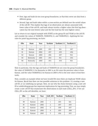
Let us consider a simple example.
Suppose that the FEMALE series is set
to display mapped values, and that
you enter the value “Female”. EViews
will examine the assigned valmap,
determine that “Female” corresponds
to the underlying value “1”, and will
assign this value to the series. Since
“1” is a valid form of numeric input,
the numeric value 1 will be placed in
the series. Note that even though we
have implicitly entered 1 into the series, the mapped spreadsheet view will continue to show
the value “Female”.
Alternatively, we could have directly entered the “1” corresponding to the underlying
numeric value. Since “1” is not a valmap label, EViews will put the value 1 in the series,
which will be displayed using the label “Female”.
While quite useful, entering data in mapped display mode requires some care, as your
results may be somewhat unexpected. For one, you should bear in mind that the required
reverse lookup of values associated with a given input requires an exact match of the input
to a label value, and a one-to-one correspondence between the given label and a valmap
value. If this condition is not met, the original input value will be placed in the series.
Consider, for example, the result of entering the string “female” instead of “Female”. In this
case, there is no matching valmap label entry, so EViews will put the input value, “female”,
into the series. Since FEMALE is a numeric series, the resulting value will be an NA, and the
display will show the mapped value for numeric missing values.
Similarly, suppose you enter “3” into the last observation of the FEMALE series. Again,
EViews does not find a corresponding valmap label entry, so the input is entered directly
into the series. In this case, the input represents a valid number so that the resulting value
will be a 3. Since there is no valmap entry for this value, the underlying value will be dis-
played.
Lastly, note that if the matching valmap label corresponds to multiple underlying values,
EViews will be unable to perform the reverse lookup. If, for example, we modify our valmap
so that the interval “[1, 10]” (instead of just the value 1) maps to the label “Female”, then](https://image.slidesharecdn.com/eviews6usersguidei-150511081027-lva1-app6892/85/E-views-6-users-guide-i-181-320.jpg)

![Value Maps—169
Valmap Functions
To facilitate working with valmaps, three new genr functions are provided which allow you
to translate between unmapped and mapped values. These functions may be used as part of
standard series or alpha expressions.
First, to obtain the mapped values corresponding to a set of numbers or strings, you may use
the command:
@map(arg[, map_name])
where arg is a numeric or string series expression or literal, and the optional map_name is
the name of a valmap object. If map_name is not provided, EViews will attempt to determine
the map by inspecting arg. This attempt will succeed only if arg is a numeric series or alpha
series that has previously been mapped.
Let us consider our original example where the FEMALEMAP maps 0 to “Male” and 1 to
“Female”. Suppose that we have two series that contain the values 0 and 1. The first series,
MAPPEDSER, has previously applied the FEMALEMAP, while the latter series, UNMAPPED-
SER, has not.
Then the commands:
alpha s1 = @map(mappedser)
alpha s2 = @map(mappedser, femalemap)
are equivalent. Both return the labels associated with the numeric values in the series. The
first command uses the assigned valmap to determine the mapped values, while the second
uses FEMALEMAP explicitly.
Alternately, the command:
alpha s3 = @map(unmappedser)
will generate an error since there is no valmap assigned to the series. To use @map in this
context, you must provide the name of a valmap, as in:
alpha s4 = @map(unmappedser, femalemap)
which will return the mapped values of UNMAPPEDSER, using the valmap FEMALEMAP.
Conversely, you may obtain the numeric values associated with a set of string value labels
using the @unmap function. The @unmap function takes the general form:
@unmap(arg, map_name)
to return the numeric values that have been mapped into the string given in the string
expression or literal arg, where map_name is the name of a valmap object. Note that if a
given label is associated with multiple numeric values, the missing value NA will be
returned. Note that the map_name argument is required with the @unmap function.](https://image.slidesharecdn.com/eviews6usersguidei-150511081027-lva1-app6892/85/E-views-6-users-guide-i-183-320.jpg)


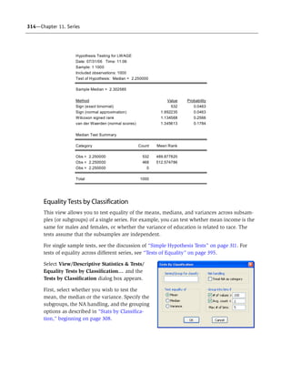


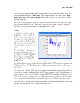
![Descriptive Statistics & Tests—317
The results show that there is strong evidence that LWAGE differs across groups defined by
MARRIED and UNION; both the standard ANOVA and the Welch adjusted ANOVA statistics
are in excess of 40, with probability values near zero.
The analysis of variance table shows the decomposition of the total sum of squares into the
between and within sum of squares, where:
Mean Sq. = Sum of Sq./df
The F-statistic is the ratio:
F = Between Mean Sq./Within Mean Sq.
The bottom portion of the output provides the category statistics:
Median (Distribution) Equality Tests
EViews computes various rank-based nonparametric tests of the hypothesis that the sub-
groups have the same general distribution, against the alternative that at least one subgroup
has a different distribution.
In the two group setting, the null hypothesis is that the two subgroups are independent sam-
ples from the same general distribution. The alternative hypothesis may loosely be defined
as “the values [of the first group] tend to differ from the values [of the second group]” (see
Conover 1980, p. 281 for discussion). See also Bergmann, Ludbrook and Spooren (2000) for
a more precise analysis of the issues involved.
We note that the “median” category in which we place these tests is somewhat misleading
since the tests focus more generally on the equality of various statistics computed across
subgroups. For example, the Wilcoxon test examines the comparability of mean ranks across
subgroups. The categorization reflects common usage for these tests and various textbook
definitions. The tests should, of course, have power against median differences.
• Wilcoxon signed ranks test. This test is computed when there are two subgroups.
The test is identical to the Wilcoxon test outlined in the description of median tests
(“Median Test” on page 313) but the division of the series into two groups is based
upon the values of the classification variable instead of the value of the observation
relative to the median.
Category Statistics
Std. Err.
UNION MARRIED Count Mean Std. Dev. of Mean
0 0 305 1.993829 0.574636 0.032904
0 1 479 2.368924 0.557405 0.025468
1 0 54 2.387019 0.395838 0.053867
1 1 162 2.492371 0.380441 0.029890
All 1000 2.275496 0.563464 0.017818](https://image.slidesharecdn.com/eviews6usersguidei-150511081027-lva1-app6892/85/E-views-6-users-guide-i-331-320.jpg)


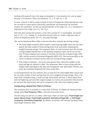
![336—Chapter 11. Series
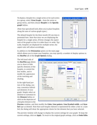
In addition to the default Index (0, 1, 2,...) method, you may elect to use the Left edges of
bins, the Right edges of bins, or the Midpoints of bins. Each of these encoding methods
should be self-explanatory. Note that index encoding is the only method available for classi-
fication by quantile values.
Value maps are not created for classifications employing non-index encoding.
NA classification
By default, observations in the original series which are NA are given the value NA in the
classification series. If you treat the NA as a category by checking Include NAs in classifica-
tion, EViews will assign NAs the index value of 0 in the classification, and will map this
value to the label “NA”.
For example, re-running our first example (step size of 100, a grid start value of 200) but
keeping NAs, we have the following raw data (note that the mapped values will be identical
to those from the earlier example):
We see that the observations 2 and 6, which were missing values in the original data, are
encoded with the index value 0.
Out-of-Range Values
You may instruct EViews to generate an error if it encounters an observation that does not
fall into one of the specified bins; by default, observations that lie outside the bin range are
simply assigned an NA.
This option is irrelevant for quantile value classification.
Right-closed Bins
Bins are left-closed by default, so that lies in the bin defined by and if . To
change the non-strict inequality from the left to the right , you must instruct
EViews to use right-closed bins by checking the box Right-closed bin intervals (a, b]. This
setting should have little effect, if any, if your data are reasonably continuous.
x a b a x b<£
a x b£<](https://image.slidesharecdn.com/eviews6usersguidei-150511081027-lva1-app6892/85/E-views-6-users-guide-i-350-320.jpg)
![Resample—337
A Couple of Warnings
In determining whether an observation is in a particular interval, EViews performs compari-
sons of real numbers to assess, for example, whether and whether . We urge
you to exercise caution in cases where and are finite precision representations of real
numbers.
To take a specific example, suppose that we wish to divide the interval from 0 to 1 into bins
of size 0.1 (so that our limit points are 0.1, 0.2, 0.3, etc.). Since 0.1 cannot be represented in
floating point by a computer, comparisons will be made with numbers that are close to, but
not exactly equal to 0.1. As a result, when there are data values approximately equal to the
limit points, classifications may behave unexpectedly since they are based on a comparison
of two floating point numbers.
A related issue occurs when you classify by number of bins, and set the start or end values
equal to the data minimum or maximum. In this situation, depending upon whether you
have selected left or right-closed intervals, observations with values equal to the start or end
may fall out-of-range.
To illustrate this issue, we extend our simple example by assuming that we wish to divide
the 0–1 range into right-closed bins. Each bin will be of the form [0.1 , 0.1 ). with
the first interval given by (0, 1]. Now consider classifying those data values that are exactly
equal to 0, and note that these values are out-of-range since they lie outside the first inter-
val. The same is true for observations equal to 1 if we have defined left-closed bins. The
comparison is more complex if the relevant endpoint is real valued since the out-of-range
status would depend upon a floating point comparison.
The obvious recommendation in this latter case are that: (1) you specify at most only one of
range start and range end at the data extremes, and (2) if you set either the start or end to
the corresponding data extreme, you define the intervals so that they are closed on the cor-
responding end (i.e., starts that equal the minimum have left-closed intervals, and ends that
equal the maximum have right-closed intervals) and you set the range so that it extends past
the other extreme. Our first example above adopts this strategy, setting the low value to the
data minimum (200), setting the steps size, and leaving the upper limit unspecified.
More generally, we urge you to exercise caution when defining intervals with real-valued
limits.
Resample
The series resampling procedure selects from the observations in a series to create a new
series (the resampled series). You may draw your new sample with replacement (allow a
given observation to be drawn multiple times) or without replacement. When you select
Proc/Resample... from the series window, you will be prompted to specify various options.
a x£ x b<
a b
i 1–( ) i](https://image.slidesharecdn.com/eviews6usersguidei-150511081027-lva1-app6892/85/E-views-6-users-guide-i-351-320.jpg)


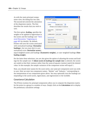
![Seasonal Adjustment—343
ARIMA Specification allows you to choose between two different methods for specifying
your ARIMA model. The Specify in-line option asks you to provide a single ARIMA specifi-
cation to fit. The X12 syntax for the ARIMA specification is different from the one used by
EViews and follows the Box-Jenkins notation “(p d q)(P D Q)” where:
The default specification “(0 1 1)(0 1 1)” is the seasonal IMA model:
(11.35)
Here are some other examples ( is the lag operator):
You can skip lags using square brackets and explicitly specify the seasonal order after the
parentheses:
See the X12-ARIMA Reference Manual (p. 110–114) for further details and examples of
ARIMA specification in X12. Note that there is a limit of 25 total AR, MA, and differencing
coefficients in a model and that the maximum lag of any AR or MA parameter is 24 and the
maximum number of differences in any ARIMA factor is 3.
Alternatively, if you choose Select from file, X12 will select an ARIMA model from a set of
possible specifications provided in an external file. The selection process is based on a pro-
cedure developed by Statistics Canada for X11-ARIMA/88 and is described in the X12-
ARIMA Reference Manual (p. 133). If you use this option, you will be asked to provide the
name of a file that contains a set of possible ARIMA specifications. By default, EViews will
p nonseasonal AR order
d order of nonseasonal differences
q nonseasonal MA order
P (multiplicative) seasonal AR order
D order of seasonal differences
Q (multiplicative) seasonal MA order
(1 0 0)
(0 1 1)
(1 0 1)(1 0 0) where
for quarterly data and for monthly
data.
([2 3] 0 0)
(0 1 1)12
1 L–( ) 1 L
s
–( )yt 1 v1L–( ) 1 vsL
s
–( )et=
L
1 fL–( )yt et=
1 L–( )yt 1 vL–( )et=
1 f1L–( ) 1 fsL
s
–( )yt 1 vL–( )et=
s 4= s 12=
1 f2L
2
– f3L
3
–( )yt et=
1 L
12
–( )yt 1 vL
12
–( )et=](https://image.slidesharecdn.com/eviews6usersguidei-150511081027-lva1-app6892/85/E-views-6-users-guide-i-357-320.jpg)


![Graph Types—485
The Bracket Bandwidth option fits three kernel regressions using bandwidths , ,
and .
For nearest neighbor (variable) bandwidths, see “Nearest Neighbor Fit,” on page 485.
Number of grid points
You must specify the number of points at which to evaluate the local polynomial regres-
sion. The default is points; you can specify any integer in the field. Suppose the
range of the series is . Then the polynomial is evaluated at equi-spaced
points:
(13.8)
Method
Given a number of evaluation points, EViews provides you with two additional computa-
tional options: exact computation and linear binning.
The Linear Binning method (Fan and Marron, 1994) approximates the kernel regression by
binning the raw data fractionally to the two nearest evaluation points, prior to evaluat-
ing the kernel estimate. For large data sets, the computational savings may be substantial,
with virtually no loss of precision.
The Exact method performs a regression at each , using all of the data points ,
for . Since the exact method computes a regression at every grid point, it
may be quite time consuming when applied to large samples. In these settings, you may
wish to consider the linear binning method.
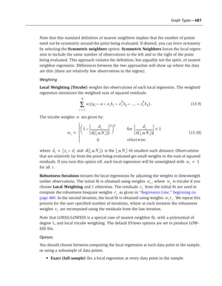
Nearest Neighbor Fit
The nearest neighbor fit displays
local polynomial regressions for
two series with bandwidth based
on nearest neighbors. Briefly, for
each data point in a sample, we fit
a locally weighted polynomial
regression. It is a local regression
since we use only the subset of
observations which lie in a neigh-
borhood of the point to fit the
regression model; it may be
weighted so that observations fur-
ther from the given data point are
given less weight.
0.5h h
1.5h
M
M 100=
X XL XU[ , ] M
xi XL i
XU XL–
M
---------------------
Ë ¯
Ê ˆ for i⋅+ 0 1 ºM 1–, ,= =
Xj
xi Xj Yj,( )
j 1 2 º N, , ,=](https://image.slidesharecdn.com/eviews6usersguidei-150511081027-lva1-app6892/85/E-views-6-users-guide-i-499-320.jpg)


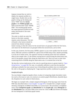


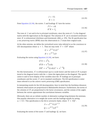
![512—Chapter 14. Categorical Graphs
To change the ordering of levels for a given fac-
tor, click on Factor and Graph Layout Options
to display the options dialog, select a factor in
the left-hand side list box, then change the Dis-
play order combo from the default Ascending
to Descending.
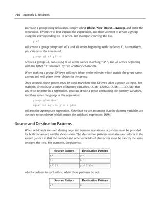
We may, for example, modify our categorical
graph for CITY_MPG using the binned values of
DISPLACEMENT. Double click on the graph to
open the main graph dialog, click on Factor and
Graph Layout Options to show the options dia-
log, and change the display order.
Note that changing the ordering of the levels
changes the order in which they are displayed
in the graph. The categories for DISPLACE-
MENT now start at the largest level for the fac-
tor and continue on through the smallest.
Multiple Factor Ordering
You may specify more than one factor variable, thereby forming a set of categories defined
by each combination of the distinct factor values. In this case, the order in which the factors
vary has an important effect on the final display.
Suppose, in addition to the FEM variable, you have a second factor variable UNION repre-
senting whether the individual is in “Union” or “Non-union” employment. Then the four
categories for these two factors are: {(“Male,” “Non-union”), (“Male,” “Union”), (“Female,”
“Non-union”), (“Female,” “Union”)}.
Note that in this list, we have arranged these factors so that:
with the “Male” categories coming first, followed by the “Female” categories, and with the
UNION status categories varying within the FEM categories. We say that the FEM factor var-
ies more slowly in this ordering than the UNION category since the latter varies within each
level of FEM.
Order FEM UNION
1 “Male” “Non-union”
2 “Male” “Union”
3 “Female” “Non-union”
4 “Female” “Union”
12
14
16
18
20
22
24
26
28
30
DISPLA
CEM
E
NT
(8,6]
DISPLA
CEM
E
NT
(6,4]
DISPLA
CEM
E
NT
(4,2]
DISPLA
CEM
E
NT
(2,0]
Mean of CITY_MPG by DISPLACEMENT](https://image.slidesharecdn.com/eviews6usersguidei-150511081027-lva1-app6892/85/E-views-6-users-guide-i-526-320.jpg)


Ad
More Related Content
What's hot (14)
Viewers also liked (11)


Ad
Similar to E views 6 users guide i (20)


Ad
Recently uploaded (20)


E views 6 users guide i
- 1. EViews 6 User’s Guide I
- 2. EViews 6 User’s Guide I Copyright © 1994–2007 Quantitative Micro Software, LLC All Rights Reserved Printed in the United States of America This software product, including program code and manual, is copyrighted, and all rights are reserved by Quantitative Micro Software, LLC. The distribution and sale of this product are intended for the use of the original purchaser only. Except as permitted under the United States Copyright Act of 1976, no part of this product may be reproduced or distributed in any form or by any means, or stored in a database or retrieval system, without the prior written permission of Quantitative Micro Software. Disclaimer The authors and Quantitative Micro Software assume no responsibility for any errors that may appear in this manual or the EViews program. The user assumes all responsibility for the selection of the program to achieve intended results, and for the installation, use, and results obtained from the program. Trademarks Windows, Windows 95/98/2000/NT/Me/XP, and Microsoft Excel are trademarks of Microsoft Corporation. PostScript is a trademark of Adobe Corporation. X11.2 and X12- ARIMA Version 0.2.7 are seasonal adjustment programs developed by the U. S. Census Bureau. Tramo/Seats is copyright by Agustin Maravall and Victor Gomez. All other product names mentioned in this manual may be trademarks or registered trademarks of their respective companies. Quantitative Micro Software, LLC 4521 Campus Drive, #336, Irvine CA, 92612-2621 Telephone: (949) 856-3368 Fax: (949) 856-2044 e-mail: [email protected] web: www.eviews.com March 9, 2007
- 3. Table of Contents EVIEWS 6 USER’S GUIDE I PREFACE . . . . . . . . . . . . . . . . . . . . . . . . . . . . . . . . . . . . . . . . . . . . . . . . . . . . . . . . . . . . . . . . . . . . 1 PART I. EVIEWS FUNDAMENTALS . . . . . . . . . . . . . . . . . . . . . . . . . . . . . . . . . . . . . . . . . . . . . . . . . 3 CHAPTER 1. INTRODUCTION . . . . . . . . . . . . . . . . . . . . . . . . . . . . . . . . . . . . . . . . . . . . . . . . . . . . . . . . . . . . 5 What is EViews? . . . . . . . . . . . . . . . . . . . . . . . . . . . . . . . . . . . . . . . . . . . . . . . . . . . . . . . . . . . 5 Installing and Running EViews . . . . . . . . . . . . . . . . . . . . . . . . . . . . . . . . . . . . . . . . . . . . . . . . . 5 Windows Basics . . . . . . . . . . . . . . . . . . . . . . . . . . . . . . . . . . . . . . . . . . . . . . . . . . . . . . . . . . . 6 The EViews Window . . . . . . . . . . . . . . . . . . . . . . . . . . . . . . . . . . . . . . . . . . . . . . . . . . . . . . . . 9 Closing EViews . . . . . . . . . . . . . . . . . . . . . . . . . . . . . . . . . . . . . . . . . . . . . . . . . . . . . . . . . . . 13 Where to Go For Help . . . . . . . . . . . . . . . . . . . . . . . . . . . . . . . . . . . . . . . . . . . . . . . . . . . . . . 13 CHAPTER 2. A DEMONSTRATION . . . . . . . . . . . . . . . . . . . . . . . . . . . . . . . . . . . . . . . . . . . . . . . . . . . . . . . 15 Getting Data into EViews . . . . . . . . . . . . . . . . . . . . . . . . . . . . . . . . . . . . . . . . . . . . . . . . . . . . 15 Examining the Data . . . . . . . . . . . . . . . . . . . . . . . . . . . . . . . . . . . . . . . . . . . . . . . . . . . . . . . . 18 Estimating a Regression Model . . . . . . . . . . . . . . . . . . . . . . . . . . . . . . . . . . . . . . . . . . . . . . . . 23 Specification and Hypothesis Tests . . . . . . . . . . . . . . . . . . . . . . . . . . . . . . . . . . . . . . . . . . . . . 26 Modifying the Equation . . . . . . . . . . . . . . . . . . . . . . . . . . . . . . . . . . . . . . . . . . . . . . . . . . . . . 28 Forecasting from an Estimated Equation . . . . . . . . . . . . . . . . . . . . . . . . . . . . . . . . . . . . . . . . . 30 Additional Testing . . . . . . . . . . . . . . . . . . . . . . . . . . . . . . . . . . . . . . . . . . . . . . . . . . . . . . . . . 34 CHAPTER 3. WORKFILE BASICS . . . . . . . . . . . . . . . . . . . . . . . . . . . . . . . . . . . . . . . . . . . . . . . . . . . . . . . . 37 What is a Workfile? . . . . . . . . . . . . . . . . . . . . . . . . . . . . . . . . . . . . . . . . . . . . . . . . . . . . . . . . 37 Creating a Workfile . . . . . . . . . . . . . . . . . . . . . . . . . . . . . . . . . . . . . . . . . . . . . . . . . . . . . . . . 38 The Workfile Window . . . . . . . . . . . . . . . . . . . . . . . . . . . . . . . . . . . . . . . . . . . . . . . . . . . . . . 46 Saving a Workfile . . . . . . . . . . . . . . . . . . . . . . . . . . . . . . . . . . . . . . . . . . . . . . . . . . . . . . . . . 50 Loading a Workfile . . . . . . . . . . . . . . . . . . . . . . . . . . . . . . . . . . . . . . . . . . . . . . . . . . . . . . . . 53 Multi-page Workfiles . . . . . . . . . . . . . . . . . . . . . . . . . . . . . . . . . . . . . . . . . . . . . . . . . . . . . . . 53 Addendum: File Dialog Features . . . . . . . . . . . . . . . . . . . . . . . . . . . . . . . . . . . . . . . . . . . . . . . 61 CHAPTER 4. OBJECT BASICS . . . . . . . . . . . . . . . . . . . . . . . . . . . . . . . . . . . . . . . . . . . . . . . . . . . . . . . . . . 63 What is an Object? . . . . . . . . . . . . . . . . . . . . . . . . . . . . . . . . . . . . . . . . . . . . . . . . . . . . . . . . 63 Basic Object Operations . . . . . . . . . . . . . . . . . . . . . . . . . . . . . . . . . . . . . . . . . . . . . . . . . . . . . 67 The Object Window . . . . . . . . . . . . . . . . . . . . . . . . . . . . . . . . . . . . . . . . . . . . . . . . . . . . . . . . 69
- 4. ii— Table of Contents Working with Objects . . . . . . . . . . . . . . . . . . . . . . . . . . . . . . . . . . . . . . . . . . . . . . . . . . . . . . .71 CHAPTER 5. BASIC DATA HANDLING . . . . . . . . . . . . . . . . . . . . . . . . . . . . . . . . . . . . . . . . . . . . . . . . . . . 77 Data Objects . . . . . . . . . . . . . . . . . . . . . . . . . . . . . . . . . . . . . . . . . . . . . . . . . . . . . . . . . . . . . .77 Samples . . . . . . . . . . . . . . . . . . . . . . . . . . . . . . . . . . . . . . . . . . . . . . . . . . . . . . . . . . . . . . . . .86 Sample Objects . . . . . . . . . . . . . . . . . . . . . . . . . . . . . . . . . . . . . . . . . . . . . . . . . . . . . . . . . . . .93 Importing Data . . . . . . . . . . . . . . . . . . . . . . . . . . . . . . . . . . . . . . . . . . . . . . . . . . . . . . . . . . . .95 Exporting Data . . . . . . . . . . . . . . . . . . . . . . . . . . . . . . . . . . . . . . . . . . . . . . . . . . . . . . . . . . .104 Frequency Conversion . . . . . . . . . . . . . . . . . . . . . . . . . . . . . . . . . . . . . . . . . . . . . . . . . . . . . .106 Importing ASCII Text Files . . . . . . . . . . . . . . . . . . . . . . . . . . . . . . . . . . . . . . . . . . . . . . . . . . .111 CHAPTER 6. WORKING WITH DATA . . . . . . . . . . . . . . . . . . . . . . . . . . . . . . . . . . . . . . . . . . . . . . . . . . . .121 Numeric Expressions . . . . . . . . . . . . . . . . . . . . . . . . . . . . . . . . . . . . . . . . . . . . . . . . . . . . . . .121 Series . . . . . . . . . . . . . . . . . . . . . . . . . . . . . . . . . . . . . . . . . . . . . . . . . . . . . . . . . . . . . . . . . .131 Auto-series . . . . . . . . . . . . . . . . . . . . . . . . . . . . . . . . . . . . . . . . . . . . . . . . . . . . . . . . . . . . . .135 Groups . . . . . . . . . . . . . . . . . . . . . . . . . . . . . . . . . . . . . . . . . . . . . . . . . . . . . . . . . . . . . . . . .139 Scalars . . . . . . . . . . . . . . . . . . . . . . . . . . . . . . . . . . . . . . . . . . . . . . . . . . . . . . . . . . . . . . . . .143 CHAPTER 7. WORKING WITH DATA (ADVANCED) . . . . . . . . . . . . . . . . . . . . . . . . . . . . . . . . . . . . . . . .145 Auto-Updating Series . . . . . . . . . . . . . . . . . . . . . . . . . . . . . . . . . . . . . . . . . . . . . . . . . . . . . . .145 Alpha Series . . . . . . . . . . . . . . . . . . . . . . . . . . . . . . . . . . . . . . . . . . . . . . . . . . . . . . . . . . . . .150 Date Series . . . . . . . . . . . . . . . . . . . . . . . . . . . . . . . . . . . . . . . . . . . . . . . . . . . . . . . . . . . . . .156 Value Maps . . . . . . . . . . . . . . . . . . . . . . . . . . . . . . . . . . . . . . . . . . . . . . . . . . . . . . . . . . . . .159 CHAPTER 8. SERIES LINKS . . . . . . . . . . . . . . . . . . . . . . . . . . . . . . . . . . . . . . . . . . . . . . . . . . . . . . . . . . . .173 Basic Link Concepts . . . . . . . . . . . . . . . . . . . . . . . . . . . . . . . . . . . . . . . . . . . . . . . . . . . . . . .173 Creating a Link . . . . . . . . . . . . . . . . . . . . . . . . . . . . . . . . . . . . . . . . . . . . . . . . . . . . . . . . . . .187 Working with Links . . . . . . . . . . . . . . . . . . . . . . . . . . . . . . . . . . . . . . . . . . . . . . . . . . . . . . .197 CHAPTER 9. ADVANCED WORKFILES . . . . . . . . . . . . . . . . . . . . . . . . . . . . . . . . . . . . . . . . . . . . . . . . . . .203 Structuring a Workfile . . . . . . . . . . . . . . . . . . . . . . . . . . . . . . . . . . . . . . . . . . . . . . . . . . . . . .203 Resizing a Workfile . . . . . . . . . . . . . . . . . . . . . . . . . . . . . . . . . . . . . . . . . . . . . . . . . . . . . . . .227 Appending to a Workfile . . . . . . . . . . . . . . . . . . . . . . . . . . . . . . . . . . . . . . . . . . . . . . . . . . . .230 Contracting a Workfile . . . . . . . . . . . . . . . . . . . . . . . . . . . . . . . . . . . . . . . . . . . . . . . . . . . . .233 Copying from a Workfile . . . . . . . . . . . . . . . . . . . . . . . . . . . . . . . . . . . . . . . . . . . . . . . . . . . .233 Reshaping a Workfile . . . . . . . . . . . . . . . . . . . . . . . . . . . . . . . . . . . . . . . . . . . . . . . . . . . . . .237 Sorting a Workfile . . . . . . . . . . . . . . . . . . . . . . . . . . . . . . . . . . . . . . . . . . . . . . . . . . . . . . . . .254 Exporting from a Workfile . . . . . . . . . . . . . . . . . . . . . . . . . . . . . . . . . . . . . . . . . . . . . . . . . . .254 References . . . . . . . . . . . . . . . . . . . . . . . . . . . . . . . . . . . . . . . . . . . . . . . . . . . . . . . . . . . . . .255
- 5. Table of Contents—iii CHAPTER 10. EVIEWS DATABASES . . . . . . . . . . . . . . . . . . . . . . . . . . . . . . . . . . . . . . . . . . . . . . . . . . . . 257 Database Overview . . . . . . . . . . . . . . . . . . . . . . . . . . . . . . . . . . . . . . . . . . . . . . . . . . . . . . . 257 Database Basics . . . . . . . . . . . . . . . . . . . . . . . . . . . . . . . . . . . . . . . . . . . . . . . . . . . . . . . . . . 258 Working with Objects in Databases . . . . . . . . . . . . . . . . . . . . . . . . . . . . . . . . . . . . . . . . . . . 262 Database Auto-Series . . . . . . . . . . . . . . . . . . . . . . . . . . . . . . . . . . . . . . . . . . . . . . . . . . . . . . 269 The Database Registry . . . . . . . . . . . . . . . . . . . . . . . . . . . . . . . . . . . . . . . . . . . . . . . . . . . . . 271 Querying the Database . . . . . . . . . . . . . . . . . . . . . . . . . . . . . . . . . . . . . . . . . . . . . . . . . . . . . 273 Object Aliases and Illegal Names . . . . . . . . . . . . . . . . . . . . . . . . . . . . . . . . . . . . . . . . . . . . . 281 Maintaining the Database . . . . . . . . . . . . . . . . . . . . . . . . . . . . . . . . . . . . . . . . . . . . . . . . . . 283 Foreign Format Databases . . . . . . . . . . . . . . . . . . . . . . . . . . . . . . . . . . . . . . . . . . . . . . . . . . 285 Working with DRIPro Links . . . . . . . . . . . . . . . . . . . . . . . . . . . . . . . . . . . . . . . . . . . . . . . . . 296 PART II. BASIC DATA ANALYSIS . . . . . . . . . . . . . . . . . . . . . . . . . . . . . . . . . . . . . . . . . . . . . . . .303 CHAPTER 11. SERIES . . . . . . . . . . . . . . . . . . . . . . . . . . . . . . . . . . . . . . . . . . . . . . . . . . . . . . . . . . . . . . . .305 Series Views Overview . . . . . . . . . . . . . . . . . . . . . . . . . . . . . . . . . . . . . . . . . . . . . . . . . . . . 305 Spreadsheet . . . . . . . . . . . . . . . . . . . . . . . . . . . . . . . . . . . . . . . . . . . . . . . . . . . . . . . . . . . . 306 Graph . . . . . . . . . . . . . . . . . . . . . . . . . . . . . . . . . . . . . . . . . . . . . . . . . . . . . . . . . . . . . . . . . 306 Descriptive Statistics & Tests . . . . . . . . . . . . . . . . . . . . . . . . . . . . . . . . . . . . . . . . . . . . . . . . 306 One-Way Tabulation . . . . . . . . . . . . . . . . . . . . . . . . . . . . . . . . . . . . . . . . . . . . . . . . . . . . . . 323 Correlogram . . . . . . . . . . . . . . . . . . . . . . . . . . . . . . . . . . . . . . . . . . . . . . . . . . . . . . . . . . . . 324 Unit Root Test . . . . . . . . . . . . . . . . . . . . . . . . . . . . . . . . . . . . . . . . . . . . . . . . . . . . . . . . . . . 327 BDS Test . . . . . . . . . . . . . . . . . . . . . . . . . . . . . . . . . . . . . . . . . . . . . . . . . . . . . . . . . . . . . . . 327 Label . . . . . . . . . . . . . . . . . . . . . . . . . . . . . . . . . . . . . . . . . . . . . . . . . . . . . . . . . . . . . . . . . 331 Properties . . . . . . . . . . . . . . . . . . . . . . . . . . . . . . . . . . . . . . . . . . . . . . . . . . . . . . . . . . . . . . 331 Series Procs Overview . . . . . . . . . . . . . . . . . . . . . . . . . . . . . . . . . . . . . . . . . . . . . . . . . . . . . 332 Generate by Equation . . . . . . . . . . . . . . . . . . . . . . . . . . . . . . . . . . . . . . . . . . . . . . . . . . . . . 332 Generate by Classification . . . . . . . . . . . . . . . . . . . . . . . . . . . . . . . . . . . . . . . . . . . . . . . . . . 333 Resample . . . . . . . . . . . . . . . . . . . . . . . . . . . . . . . . . . . . . . . . . . . . . . . . . . . . . . . . . . . . . . 337 Seasonal Adjustment . . . . . . . . . . . . . . . . . . . . . . . . . . . . . . . . . . . . . . . . . . . . . . . . . . . . . . 339 Exponential Smoothing . . . . . . . . . . . . . . . . . . . . . . . . . . . . . . . . . . . . . . . . . . . . . . . . . . . . 354 Hodrick-Prescott Filter . . . . . . . . . . . . . . . . . . . . . . . . . . . . . . . . . . . . . . . . . . . . . . . . . . . . . 360 Frequency (Band-Pass) Filter . . . . . . . . . . . . . . . . . . . . . . . . . . . . . . . . . . . . . . . . . . . . . . . . 361 References . . . . . . . . . . . . . . . . . . . . . . . . . . . . . . . . . . . . . . . . . . . . . . . . . . . . . . . . . . . . . 365 CHAPTER 12. GROUPS . . . . . . . . . . . . . . . . . . . . . . . . . . . . . . . . . . . . . . . . . . . . . . . . . . . . . . . . . . . . . . 367 Group Views Overview . . . . . . . . . . . . . . . . . . . . . . . . . . . . . . . . . . . . . . . . . . . . . . . . . . . . 367
- 6. iv— Table of Contents Group Members . . . . . . . . . . . . . . . . . . . . . . . . . . . . . . . . . . . . . . . . . . . . . . . . . . . . . . . . . .367 Spreadsheet . . . . . . . . . . . . . . . . . . . . . . . . . . . . . . . . . . . . . . . . . . . . . . . . . . . . . . . . . . . . .368 Dated Data Table . . . . . . . . . . . . . . . . . . . . . . . . . . . . . . . . . . . . . . . . . . . . . . . . . . . . . . . . .370 Graph . . . . . . . . . . . . . . . . . . . . . . . . . . . . . . . . . . . . . . . . . . . . . . . . . . . . . . . . . . . . . . . . . .379 Descriptive Statistics . . . . . . . . . . . . . . . . . . . . . . . . . . . . . . . . . . . . . . . . . . . . . . . . . . . . . . .379 Covariance Analysis . . . . . . . . . . . . . . . . . . . . . . . . . . . . . . . . . . . . . . . . . . . . . . . . . . . . . . .380 N-Way Tabulation . . . . . . . . . . . . . . . . . . . . . . . . . . . . . . . . . . . . . . . . . . . . . . . . . . . . . . . .392 Tests of Equality . . . . . . . . . . . . . . . . . . . . . . . . . . . . . . . . . . . . . . . . . . . . . . . . . . . . . . . . . .395 Principal Components . . . . . . . . . . . . . . . . . . . . . . . . . . . . . . . . . . . . . . . . . . . . . . . . . . . . . .397 Correlograms . . . . . . . . . . . . . . . . . . . . . . . . . . . . . . . . . . . . . . . . . . . . . . . . . . . . . . . . . . . .409 Cross Correlations and Correlograms . . . . . . . . . . . . . . . . . . . . . . . . . . . . . . . . . . . . . . . . . . .409 Cointegration Test . . . . . . . . . . . . . . . . . . . . . . . . . . . . . . . . . . . . . . . . . . . . . . . . . . . . . . . . .410 Unit Root Test . . . . . . . . . . . . . . . . . . . . . . . . . . . . . . . . . . . . . . . . . . . . . . . . . . . . . . . . . . .410 Granger Causality . . . . . . . . . . . . . . . . . . . . . . . . . . . . . . . . . . . . . . . . . . . . . . . . . . . . . . . . .410 Label . . . . . . . . . . . . . . . . . . . . . . . . . . . . . . . . . . . . . . . . . . . . . . . . . . . . . . . . . . . . . . . . . .412 Group Procedures Overview . . . . . . . . . . . . . . . . . . . . . . . . . . . . . . . . . . . . . . . . . . . . . . . . .412 References . . . . . . . . . . . . . . . . . . . . . . . . . . . . . . . . . . . . . . . . . . . . . . . . . . . . . . . . . . . . . .413 CHAPTER 13. GRAPHING DATA . . . . . . . . . . . . . . . . . . . . . . . . . . . . . . . . . . . . . . . . . . . . . . . . . . . . . . .415 Quick Start . . . . . . . . . . . . . . . . . . . . . . . . . . . . . . . . . . . . . . . . . . . . . . . . . . . . . . . . . . . . . .416 Graphing a Series . . . . . . . . . . . . . . . . . . . . . . . . . . . . . . . . . . . . . . . . . . . . . . . . . . . . . . . . .419 Graphing Multiple Series (Groups) . . . . . . . . . . . . . . . . . . . . . . . . . . . . . . . . . . . . . . . . . . . . .427 Basic Customization . . . . . . . . . . . . . . . . . . . . . . . . . . . . . . . . . . . . . . . . . . . . . . . . . . . . . . .438 Graph Types . . . . . . . . . . . . . . . . . . . . . . . . . . . . . . . . . . . . . . . . . . . . . . . . . . . . . . . . . . . . .449 References . . . . . . . . . . . . . . . . . . . . . . . . . . . . . . . . . . . . . . . . . . . . . . . . . . . . . . . . . . . . . .490 CHAPTER 14. CATEGORICAL GRAPHS . . . . . . . . . . . . . . . . . . . . . . . . . . . . . . . . . . . . . . . . . . . . . . . . . .491 Illustrative Examples . . . . . . . . . . . . . . . . . . . . . . . . . . . . . . . . . . . . . . . . . . . . . . . . . . . . . . .491 Specifying Factors . . . . . . . . . . . . . . . . . . . . . . . . . . . . . . . . . . . . . . . . . . . . . . . . . . . . . . . . .508 CHAPTER 15. GRAPHS, TABLES, TEXT, AND SPOOLS . . . . . . . . . . . . . . . . . . . . . . . . . . . . . . . . . . . . . .523 Background . . . . . . . . . . . . . . . . . . . . . . . . . . . . . . . . . . . . . . . . . . . . . . . . . . . . . . . . . . . . .523 Graph Objects . . . . . . . . . . . . . . . . . . . . . . . . . . . . . . . . . . . . . . . . . . . . . . . . . . . . . . . . . . . .523 Table Objects . . . . . . . . . . . . . . . . . . . . . . . . . . . . . . . . . . . . . . . . . . . . . . . . . . . . . . . . . . . .545 Text Objects . . . . . . . . . . . . . . . . . . . . . . . . . . . . . . . . . . . . . . . . . . . . . . . . . . . . . . . . . . . . .554 Spool Objects . . . . . . . . . . . . . . . . . . . . . . . . . . . . . . . . . . . . . . . . . . . . . . . . . . . . . . . . . . . .554
- 7. Table of Contents—v PART III. COMMANDS AND PROGRAMMING . . . . . . . . . . . . . . . . . . . . . . . . . . . . . . . . . . . . . .575 CHAPTER 16. OBJECT AND COMMAND BASICS . . . . . . . . . . . . . . . . . . . . . . . . . . . . . . . . . . . . . . . . . . 577 Using Commands . . . . . . . . . . . . . . . . . . . . . . . . . . . . . . . . . . . . . . . . . . . . . . . . . . . . . . . . 577 Object Declaration and Initialization . . . . . . . . . . . . . . . . . . . . . . . . . . . . . . . . . . . . . . . . . . . 578 Object Commands . . . . . . . . . . . . . . . . . . . . . . . . . . . . . . . . . . . . . . . . . . . . . . . . . . . . . . . . 582 Interactive Commands . . . . . . . . . . . . . . . . . . . . . . . . . . . . . . . . . . . . . . . . . . . . . . . . . . . . . 585 Auxiliary Commands . . . . . . . . . . . . . . . . . . . . . . . . . . . . . . . . . . . . . . . . . . . . . . . . . . . . . . 586 CHAPTER 17. EVIEWS PROGRAMMING . . . . . . . . . . . . . . . . . . . . . . . . . . . . . . . . . . . . . . . . . . . . . . . . . 593 Program Basics . . . . . . . . . . . . . . . . . . . . . . . . . . . . . . . . . . . . . . . . . . . . . . . . . . . . . . . . . . 593 Simple Programs . . . . . . . . . . . . . . . . . . . . . . . . . . . . . . . . . . . . . . . . . . . . . . . . . . . . . . . . . 596 Program Variables . . . . . . . . . . . . . . . . . . . . . . . . . . . . . . . . . . . . . . . . . . . . . . . . . . . . . . . . 598 Program Modes . . . . . . . . . . . . . . . . . . . . . . . . . . . . . . . . . . . . . . . . . . . . . . . . . . . . . . . . . . 607 Program Arguments . . . . . . . . . . . . . . . . . . . . . . . . . . . . . . . . . . . . . . . . . . . . . . . . . . . . . . 608 Control of Execution . . . . . . . . . . . . . . . . . . . . . . . . . . . . . . . . . . . . . . . . . . . . . . . . . . . . . . 610 Multiple Program Files . . . . . . . . . . . . . . . . . . . . . . . . . . . . . . . . . . . . . . . . . . . . . . . . . . . . . 618 Subroutines . . . . . . . . . . . . . . . . . . . . . . . . . . . . . . . . . . . . . . . . . . . . . . . . . . . . . . . . . . . . . 619 CHAPTER 18. MATRIX LANGUAGE . . . . . . . . . . . . . . . . . . . . . . . . . . . . . . . . . . . . . . . . . . . . . . . . . . . . .627 Declaring Matrix Objects . . . . . . . . . . . . . . . . . . . . . . . . . . . . . . . . . . . . . . . . . . . . . . . . . . . 627 Assigning Matrix Values . . . . . . . . . . . . . . . . . . . . . . . . . . . . . . . . . . . . . . . . . . . . . . . . . . . 628 Copying Data Between Objects . . . . . . . . . . . . . . . . . . . . . . . . . . . . . . . . . . . . . . . . . . . . . . . 631 Matrix Expressions . . . . . . . . . . . . . . . . . . . . . . . . . . . . . . . . . . . . . . . . . . . . . . . . . . . . . . . 638 Matrix Commands and Functions . . . . . . . . . . . . . . . . . . . . . . . . . . . . . . . . . . . . . . . . . . . . . 641 Matrix Views and Procs . . . . . . . . . . . . . . . . . . . . . . . . . . . . . . . . . . . . . . . . . . . . . . . . . . . . 645 Matrix Operations versus Loop Operations . . . . . . . . . . . . . . . . . . . . . . . . . . . . . . . . . . . . . . 647 Summary of Automatic Resizing of Matrix Objects . . . . . . . . . . . . . . . . . . . . . . . . . . . . . . . . 648 CHAPTER 19. WORKING WITH GRAPHS . . . . . . . . . . . . . . . . . . . . . . . . . . . . . . . . . . . . . . . . . . . . . . . . 651 Creating a Graph . . . . . . . . . . . . . . . . . . . . . . . . . . . . . . . . . . . . . . . . . . . . . . . . . . . . . . . . . 651 Changing Graph Types . . . . . . . . . . . . . . . . . . . . . . . . . . . . . . . . . . . . . . . . . . . . . . . . . . . . 655 Customizing a Graph . . . . . . . . . . . . . . . . . . . . . . . . . . . . . . . . . . . . . . . . . . . . . . . . . . . . . . 656 Labeling Graphs . . . . . . . . . . . . . . . . . . . . . . . . . . . . . . . . . . . . . . . . . . . . . . . . . . . . . . . . . 672 Printing Graphs . . . . . . . . . . . . . . . . . . . . . . . . . . . . . . . . . . . . . . . . . . . . . . . . . . . . . . . . . . 673 Exporting Graphs to Files . . . . . . . . . . . . . . . . . . . . . . . . . . . . . . . . . . . . . . . . . . . . . . . . . . . 673 Graph Summary . . . . . . . . . . . . . . . . . . . . . . . . . . . . . . . . . . . . . . . . . . . . . . . . . . . . . . . . . 674
- 8. vi— Table of Contents CHAPTER 20. WORKING WITH TABLES . . . . . . . . . . . . . . . . . . . . . . . . . . . . . . . . . . . . . . . . . . . . . . . . .675 Creating a Table . . . . . . . . . . . . . . . . . . . . . . . . . . . . . . . . . . . . . . . . . . . . . . . . . . . . . . . . . .675 Assigning Table Values . . . . . . . . . . . . . . . . . . . . . . . . . . . . . . . . . . . . . . . . . . . . . . . . . . . . .676 Customizing Tables . . . . . . . . . . . . . . . . . . . . . . . . . . . . . . . . . . . . . . . . . . . . . . . . . . . . . . . .678 Labeling Tables . . . . . . . . . . . . . . . . . . . . . . . . . . . . . . . . . . . . . . . . . . . . . . . . . . . . . . . . . . .684 Printing Tables . . . . . . . . . . . . . . . . . . . . . . . . . . . . . . . . . . . . . . . . . . . . . . . . . . . . . . . . . . .684 Exporting Tables to Files . . . . . . . . . . . . . . . . . . . . . . . . . . . . . . . . . . . . . . . . . . . . . . . . . . . .684 Customizing Spreadsheet Views . . . . . . . . . . . . . . . . . . . . . . . . . . . . . . . . . . . . . . . . . . . . . . .685 Table Summary . . . . . . . . . . . . . . . . . . . . . . . . . . . . . . . . . . . . . . . . . . . . . . . . . . . . . . . . . .686 CHAPTER 21. WORKING WITH SPOOLS . . . . . . . . . . . . . . . . . . . . . . . . . . . . . . . . . . . . . . . . . . . . . . . . .687 Creating a Spool . . . . . . . . . . . . . . . . . . . . . . . . . . . . . . . . . . . . . . . . . . . . . . . . . . . . . . . . . .687 Working with a Spool . . . . . . . . . . . . . . . . . . . . . . . . . . . . . . . . . . . . . . . . . . . . . . . . . . . . . .687 Printing the Spool . . . . . . . . . . . . . . . . . . . . . . . . . . . . . . . . . . . . . . . . . . . . . . . . . . . . . . . . .692 Spool Summary . . . . . . . . . . . . . . . . . . . . . . . . . . . . . . . . . . . . . . . . . . . . . . . . . . . . . . . . . .693 CHAPTER 22. STRINGS AND DATES . . . . . . . . . . . . . . . . . . . . . . . . . . . . . . . . . . . . . . . . . . . . . . . . . . . .695 Strings . . . . . . . . . . . . . . . . . . . . . . . . . . . . . . . . . . . . . . . . . . . . . . . . . . . . . . . . . . . . . . . . .695 Dates . . . . . . . . . . . . . . . . . . . . . . . . . . . . . . . . . . . . . . . . . . . . . . . . . . . . . . . . . . . . . . . . . .704 CHAPTER 23. WORKFILE FUNCTIONS . . . . . . . . . . . . . . . . . . . . . . . . . . . . . . . . . . . . . . . . . . . . . . . . . .727 Basic Workfile Information . . . . . . . . . . . . . . . . . . . . . . . . . . . . . . . . . . . . . . . . . . . . . . . . . .727 Dated Workfile Information . . . . . . . . . . . . . . . . . . . . . . . . . . . . . . . . . . . . . . . . . . . . . . . . . .728 Panel Workfile Functions . . . . . . . . . . . . . . . . . . . . . . . . . . . . . . . . . . . . . . . . . . . . . . . . . . .731 APPENDIX A. OPERATOR AND FUNCTION REFERENCE . . . . . . . . . . . . . . . . . . . . . . . . . . . . . . . . . . . . .733 Operators . . . . . . . . . . . . . . . . . . . . . . . . . . . . . . . . . . . . . . . . . . . . . . . . . . . . . . . . . . . . . . .734 Basic Mathematical Functions . . . . . . . . . . . . . . . . . . . . . . . . . . . . . . . . . . . . . . . . . . . . . . . .735 Time Series Functions . . . . . . . . . . . . . . . . . . . . . . . . . . . . . . . . . . . . . . . . . . . . . . . . . . . . . .736 Financial Functions . . . . . . . . . . . . . . . . . . . . . . . . . . . . . . . . . . . . . . . . . . . . . . . . . . . . . . . .737 Descriptive Statistics . . . . . . . . . . . . . . . . . . . . . . . . . . . . . . . . . . . . . . . . . . . . . . . . . . . . . . .738 Cumulative Statistic Functions . . . . . . . . . . . . . . . . . . . . . . . . . . . . . . . . . . . . . . . . . . . . . . . .741 Moving Statistic Functions . . . . . . . . . . . . . . . . . . . . . . . . . . . . . . . . . . . . . . . . . . . . . . . . . . .743 Group Row Functions . . . . . . . . . . . . . . . . . . . . . . . . . . . . . . . . . . . . . . . . . . . . . . . . . . . . . .748 By-Group Statistics . . . . . . . . . . . . . . . . . . . . . . . . . . . . . . . . . . . . . . . . . . . . . . . . . . . . . . . .749 Special Functions . . . . . . . . . . . . . . . . . . . . . . . . . . . . . . . . . . . . . . . . . . . . . . . . . . . . . . . . .751 Trigonometric Functions . . . . . . . . . . . . . . . . . . . . . . . . . . . . . . . . . . . . . . . . . . . . . . . . . . . .754 Statistical Distribution Functions . . . . . . . . . . . . . . . . . . . . . . . . . . . . . . . . . . . . . . . . . . . . . .754
- 9. Table of Contents—vii String Functions . . . . . . . . . . . . . . . . . . . . . . . . . . . . . . . . . . . . . . . . . . . . . . . . . . . . . . . . . 758 Date Functions . . . . . . . . . . . . . . . . . . . . . . . . . . . . . . . . . . . . . . . . . . . . . . . . . . . . . . . . . . 759 Workfile Functions . . . . . . . . . . . . . . . . . . . . . . . . . . . . . . . . . . . . . . . . . . . . . . . . . . . . . . . 760 Valmap Functions . . . . . . . . . . . . . . . . . . . . . . . . . . . . . . . . . . . . . . . . . . . . . . . . . . . . . . . . 762 References . . . . . . . . . . . . . . . . . . . . . . . . . . . . . . . . . . . . . . . . . . . . . . . . . . . . . . . . . . . . . 762 APPENDIX B. GLOBAL OPTIONS . . . . . . . . . . . . . . . . . . . . . . . . . . . . . . . . . . . . . . . . . . . . . . . . . . . . . .763 The Options Menu . . . . . . . . . . . . . . . . . . . . . . . . . . . . . . . . . . . . . . . . . . . . . . . . . . . . . . . . 763 Print Setup . . . . . . . . . . . . . . . . . . . . . . . . . . . . . . . . . . . . . . . . . . . . . . . . . . . . . . . . . . . . . 771 APPENDIX C. WILDCARDS . . . . . . . . . . . . . . . . . . . . . . . . . . . . . . . . . . . . . . . . . . . . . . . . . . . . . . . . . . . 775 Wildcard Expressions . . . . . . . . . . . . . . . . . . . . . . . . . . . . . . . . . . . . . . . . . . . . . . . . . . . . . 775 Using Wildcard Expressions . . . . . . . . . . . . . . . . . . . . . . . . . . . . . . . . . . . . . . . . . . . . . . . . . 775 Source and Destination Patterns . . . . . . . . . . . . . . . . . . . . . . . . . . . . . . . . . . . . . . . . . . . . . . 776 Resolving Ambiguities . . . . . . . . . . . . . . . . . . . . . . . . . . . . . . . . . . . . . . . . . . . . . . . . . . . . . 777 Wildcard versus Pool Identifier . . . . . . . . . . . . . . . . . . . . . . . . . . . . . . . . . . . . . . . . . . . . . . 778 EVIEWS 6 USER’S GUIDE II PREFACE . . . . . . . . . . . . . . . . . . . . . . . . . . . . . . . . . . . . . . . . . . . . . . . . . . . . . . . . . . . . . . . . . . . . 1 PART IV. BASIC SINGLE EQUATION ANALYSIS . . . . . . . . . . . . . . . . . . . . . . . . . . . . . . . . . . . . . . . 3 CHAPTER 24. BASIC REGRESSION . . . . . . . . . . . . . . . . . . . . . . . . . . . . . . . . . . . . . . . . . . . . . . . . . . . . . . . 5 Equation Objects . . . . . . . . . . . . . . . . . . . . . . . . . . . . . . . . . . . . . . . . . . . . . . . . . . . . . . . . . . . 5 Specifying an Equation in EViews . . . . . . . . . . . . . . . . . . . . . . . . . . . . . . . . . . . . . . . . . . . . . . 6 Estimating an Equation in EViews . . . . . . . . . . . . . . . . . . . . . . . . . . . . . . . . . . . . . . . . . . . . . . 9 Equation Output . . . . . . . . . . . . . . . . . . . . . . . . . . . . . . . . . . . . . . . . . . . . . . . . . . . . . . . . . . 11 Working with Equations . . . . . . . . . . . . . . . . . . . . . . . . . . . . . . . . . . . . . . . . . . . . . . . . . . . . 17 Estimation Problems . . . . . . . . . . . . . . . . . . . . . . . . . . . . . . . . . . . . . . . . . . . . . . . . . . . . . . . 21 References . . . . . . . . . . . . . . . . . . . . . . . . . . . . . . . . . . . . . . . . . . . . . . . . . . . . . . . . . . . . . . 22 CHAPTER 25. ADDITIONAL REGRESSION METHODS . . . . . . . . . . . . . . . . . . . . . . . . . . . . . . . . . . . . . . . . 23 Special Equation Terms . . . . . . . . . . . . . . . . . . . . . . . . . . . . . . . . . . . . . . . . . . . . . . . . . . . . . 23 Weighted Least Squares . . . . . . . . . . . . . . . . . . . . . . . . . . . . . . . . . . . . . . . . . . . . . . . . . . . . . 32 Heteroskedasticity and Autocorrelation Consistent Covariances . . . . . . . . . . . . . . . . . . . . . . . . 35 Two-stage Least Squares . . . . . . . . . . . . . . . . . . . . . . . . . . . . . . . . . . . . . . . . . . . . . . . . . . . . 37 Nonlinear Least Squares . . . . . . . . . . . . . . . . . . . . . . . . . . . . . . . . . . . . . . . . . . . . . . . . . . . . 43 Generalized Method of Moments (GMM) . . . . . . . . . . . . . . . . . . . . . . . . . . . . . . . . . . . . . . . . 51
- 10. viii— Table of Contents Stepwise Least Squares Regression . . . . . . . . . . . . . . . . . . . . . . . . . . . . . . . . . . . . . . . . . . . . . .55 References . . . . . . . . . . . . . . . . . . . . . . . . . . . . . . . . . . . . . . . . . . . . . . . . . . . . . . . . . . . . . . .62 CHAPTER 26. TIME SERIES REGRESSION . . . . . . . . . . . . . . . . . . . . . . . . . . . . . . . . . . . . . . . . . . . . . . . . . 63 Serial Correlation Theory . . . . . . . . . . . . . . . . . . . . . . . . . . . . . . . . . . . . . . . . . . . . . . . . . . . . .63 Testing for Serial Correlation . . . . . . . . . . . . . . . . . . . . . . . . . . . . . . . . . . . . . . . . . . . . . . . . . .64 Estimating AR Models . . . . . . . . . . . . . . . . . . . . . . . . . . . . . . . . . . . . . . . . . . . . . . . . . . . . . . .67 ARIMA Theory . . . . . . . . . . . . . . . . . . . . . . . . . . . . . . . . . . . . . . . . . . . . . . . . . . . . . . . . . . . .71 Estimating ARIMA Models . . . . . . . . . . . . . . . . . . . . . . . . . . . . . . . . . . . . . . . . . . . . . . . . . . . .73 ARMA Equation Diagnostics . . . . . . . . . . . . . . . . . . . . . . . . . . . . . . . . . . . . . . . . . . . . . . . . . .83 Nonstationary Time Series . . . . . . . . . . . . . . . . . . . . . . . . . . . . . . . . . . . . . . . . . . . . . . . . . . . .87 Unit Root Tests . . . . . . . . . . . . . . . . . . . . . . . . . . . . . . . . . . . . . . . . . . . . . . . . . . . . . . . . . . . .88 Panel Unit Root Tests . . . . . . . . . . . . . . . . . . . . . . . . . . . . . . . . . . . . . . . . . . . . . . . . . . . . . .100 References . . . . . . . . . . . . . . . . . . . . . . . . . . . . . . . . . . . . . . . . . . . . . . . . . . . . . . . . . . . . . .111 CHAPTER 27. FORECASTING FROM AN EQUATION . . . . . . . . . . . . . . . . . . . . . . . . . . . . . . . . . . . . . . . .113 Forecasting from Equations in EViews . . . . . . . . . . . . . . . . . . . . . . . . . . . . . . . . . . . . . . . . . .113 An Illustration . . . . . . . . . . . . . . . . . . . . . . . . . . . . . . . . . . . . . . . . . . . . . . . . . . . . . . . . . . .116 Forecast Basics . . . . . . . . . . . . . . . . . . . . . . . . . . . . . . . . . . . . . . . . . . . . . . . . . . . . . . . . . . .119 Forecasts with Lagged Dependent Variables . . . . . . . . . . . . . . . . . . . . . . . . . . . . . . . . . . . . . .125 Forecasting with ARMA Errors . . . . . . . . . . . . . . . . . . . . . . . . . . . . . . . . . . . . . . . . . . . . . . . .127 Forecasting from Equations with Expressions . . . . . . . . . . . . . . . . . . . . . . . . . . . . . . . . . . . . .132 Forecasting with Nonlinear and PDL Specifications . . . . . . . . . . . . . . . . . . . . . . . . . . . . . . . . .138 References . . . . . . . . . . . . . . . . . . . . . . . . . . . . . . . . . . . . . . . . . . . . . . . . . . . . . . . . . . . . . .139 CHAPTER 28. SPECIFICATION AND DIAGNOSTIC TESTS . . . . . . . . . . . . . . . . . . . . . . . . . . . . . . . . . . . .141 Background . . . . . . . . . . . . . . . . . . . . . . . . . . . . . . . . . . . . . . . . . . . . . . . . . . . . . . . . . . . . .141 Coefficient Tests . . . . . . . . . . . . . . . . . . . . . . . . . . . . . . . . . . . . . . . . . . . . . . . . . . . . . . . . . .142 Residual Tests . . . . . . . . . . . . . . . . . . . . . . . . . . . . . . . . . . . . . . . . . . . . . . . . . . . . . . . . . . . .154 Specification and Stability Tests . . . . . . . . . . . . . . . . . . . . . . . . . . . . . . . . . . . . . . . . . . . . . . .164 Applications . . . . . . . . . . . . . . . . . . . . . . . . . . . . . . . . . . . . . . . . . . . . . . . . . . . . . . . . . . . . .176 References . . . . . . . . . . . . . . . . . . . . . . . . . . . . . . . . . . . . . . . . . . . . . . . . . . . . . . . . . . . . . .180 PART V. ADVANCED SINGLE EQUATION ANALYSIS . . . . . . . . . . . . . . . . . . . . . . . . . . . . . . . .183 CHAPTER 29. ARCH AND GARCH ESTIMATION . . . . . . . . . . . . . . . . . . . . . . . . . . . . . . . . . . . . . . . . .185 Basic ARCH Specifications . . . . . . . . . . . . . . . . . . . . . . . . . . . . . . . . . . . . . . . . . . . . . . . . . . .185 Estimating ARCH Models in EViews . . . . . . . . . . . . . . . . . . . . . . . . . . . . . . . . . . . . . . . . . . . .188 Working with ARCH Models . . . . . . . . . . . . . . . . . . . . . . . . . . . . . . . . . . . . . . . . . . . . . . . . .195
- 11. Table of Contents—ix Additional ARCH Models . . . . . . . . . . . . . . . . . . . . . . . . . . . . . . . . . . . . . . . . . . . . . . . . . . . 197 Examples . . . . . . . . . . . . . . . . . . . . . . . . . . . . . . . . . . . . . . . . . . . . . . . . . . . . . . . . . . . . . . 202 References . . . . . . . . . . . . . . . . . . . . . . . . . . . . . . . . . . . . . . . . . . . . . . . . . . . . . . . . . . . . . 206 CHAPTER 30. DISCRETE AND LIMITED DEPENDENT VARIABLE MODELS . . . . . . . . . . . . . . . . . . . . . . . 209 Binary Dependent Variable Models . . . . . . . . . . . . . . . . . . . . . . . . . . . . . . . . . . . . . . . . . . . . 209 Ordered Dependent Variable Models . . . . . . . . . . . . . . . . . . . . . . . . . . . . . . . . . . . . . . . . . . 226 Censored Regression Models . . . . . . . . . . . . . . . . . . . . . . . . . . . . . . . . . . . . . . . . . . . . . . . . 232 Truncated Regression Models . . . . . . . . . . . . . . . . . . . . . . . . . . . . . . . . . . . . . . . . . . . . . . . . 242 Count Models . . . . . . . . . . . . . . . . . . . . . . . . . . . . . . . . . . . . . . . . . . . . . . . . . . . . . . . . . . . 246 Technical Notes . . . . . . . . . . . . . . . . . . . . . . . . . . . . . . . . . . . . . . . . . . . . . . . . . . . . . . . . . 255 References . . . . . . . . . . . . . . . . . . . . . . . . . . . . . . . . . . . . . . . . . . . . . . . . . . . . . . . . . . . . . 257 CHAPTER 31. QUANTILE REGRESSION . . . . . . . . . . . . . . . . . . . . . . . . . . . . . . . . . . . . . . . . . . . . . . . . . . 259 Estimating Quantile Regression in EViews . . . . . . . . . . . . . . . . . . . . . . . . . . . . . . . . . . . . . . 259 Views and Procedures . . . . . . . . . . . . . . . . . . . . . . . . . . . . . . . . . . . . . . . . . . . . . . . . . . . . . 265 Background . . . . . . . . . . . . . . . . . . . . . . . . . . . . . . . . . . . . . . . . . . . . . . . . . . . . . . . . . . . . . 270 References . . . . . . . . . . . . . . . . . . . . . . . . . . . . . . . . . . . . . . . . . . . . . . . . . . . . . . . . . . . . . 281 CHAPTER 32. THE LOG LIKELIHOOD (LOGL) OBJECT . . . . . . . . . . . . . . . . . . . . . . . . . . . . . . . . . . . . . 283 Overview . . . . . . . . . . . . . . . . . . . . . . . . . . . . . . . . . . . . . . . . . . . . . . . . . . . . . . . . . . . . . . 283 Specification . . . . . . . . . . . . . . . . . . . . . . . . . . . . . . . . . . . . . . . . . . . . . . . . . . . . . . . . . . . . 285 Estimation . . . . . . . . . . . . . . . . . . . . . . . . . . . . . . . . . . . . . . . . . . . . . . . . . . . . . . . . . . . . . 290 LogL Views . . . . . . . . . . . . . . . . . . . . . . . . . . . . . . . . . . . . . . . . . . . . . . . . . . . . . . . . . . . . . 292 LogL Procs . . . . . . . . . . . . . . . . . . . . . . . . . . . . . . . . . . . . . . . . . . . . . . . . . . . . . . . . . . . . . 293 Troubleshooting . . . . . . . . . . . . . . . . . . . . . . . . . . . . . . . . . . . . . . . . . . . . . . . . . . . . . . . . . 296 Limitations . . . . . . . . . . . . . . . . . . . . . . . . . . . . . . . . . . . . . . . . . . . . . . . . . . . . . . . . . . . . . 297 Examples . . . . . . . . . . . . . . . . . . . . . . . . . . . . . . . . . . . . . . . . . . . . . . . . . . . . . . . . . . . . . . 298 References . . . . . . . . . . . . . . . . . . . . . . . . . . . . . . . . . . . . . . . . . . . . . . . . . . . . . . . . . . . . . 304 PART VI. MULTIPLE EQUATION ANALYSIS . . . . . . . . . . . . . . . . . . . . . . . . . . . . . . . . . . . . . . . .305 CHAPTER 33. SYSTEM ESTIMATION . . . . . . . . . . . . . . . . . . . . . . . . . . . . . . . . . . . . . . . . . . . . . . . . . . . . 307 Background . . . . . . . . . . . . . . . . . . . . . . . . . . . . . . . . . . . . . . . . . . . . . . . . . . . . . . . . . . . . . 307 System Estimation Methods . . . . . . . . . . . . . . . . . . . . . . . . . . . . . . . . . . . . . . . . . . . . . . . . . 308 How to Create and Specify a System . . . . . . . . . . . . . . . . . . . . . . . . . . . . . . . . . . . . . . . . . . . 310 Working With Systems . . . . . . . . . . . . . . . . . . . . . . . . . . . . . . . . . . . . . . . . . . . . . . . . . . . . 321 Technical Discussion . . . . . . . . . . . . . . . . . . . . . . . . . . . . . . . . . . . . . . . . . . . . . . . . . . . . . . 333 References . . . . . . . . . . . . . . . . . . . . . . . . . . . . . . . . . . . . . . . . . . . . . . . . . . . . . . . . . . . . . 343
- 12. x— Table of Contents CHAPTER 34. VECTOR AUTOREGRESSION AND ERROR CORRECTION MODELS . . . . . . . . . . . . . . . . . .345 Vector Autoregressions (VARs) . . . . . . . . . . . . . . . . . . . . . . . . . . . . . . . . . . . . . . . . . . . . . . .345 Estimating a VAR in EViews . . . . . . . . . . . . . . . . . . . . . . . . . . . . . . . . . . . . . . . . . . . . . . . . .346 VAR Estimation Output . . . . . . . . . . . . . . . . . . . . . . . . . . . . . . . . . . . . . . . . . . . . . . . . . . . . .346 Views and Procs of a VAR . . . . . . . . . . . . . . . . . . . . . . . . . . . . . . . . . . . . . . . . . . . . . . . . . . .348 Structural (Identified) VARs . . . . . . . . . . . . . . . . . . . . . . . . . . . . . . . . . . . . . . . . . . . . . . . . . .357 Cointegration Testing . . . . . . . . . . . . . . . . . . . . . . . . . . . . . . . . . . . . . . . . . . . . . . . . . . . . . .363 Panel Cointegration Testing . . . . . . . . . . . . . . . . . . . . . . . . . . . . . . . . . . . . . . . . . . . . . . . . . .372 Vector Error Correction (VEC) Models . . . . . . . . . . . . . . . . . . . . . . . . . . . . . . . . . . . . . . . . . .377 A Note on Version Compatibility . . . . . . . . . . . . . . . . . . . . . . . . . . . . . . . . . . . . . . . . . . . . . .381 References . . . . . . . . . . . . . . . . . . . . . . . . . . . . . . . . . . . . . . . . . . . . . . . . . . . . . . . . . . . . . .381 CHAPTER 35. STATE SPACE MODELS AND THE KALMAN FILTER . . . . . . . . . . . . . . . . . . . . . . . . . . . . .383 Background . . . . . . . . . . . . . . . . . . . . . . . . . . . . . . . . . . . . . . . . . . . . . . . . . . . . . . . . . . . . .383 Specifying a State Space Model in EViews . . . . . . . . . . . . . . . . . . . . . . . . . . . . . . . . . . . . . . .388 Working with the State Space . . . . . . . . . . . . . . . . . . . . . . . . . . . . . . . . . . . . . . . . . . . . . . . .399 Converting from Version 3 Sspace . . . . . . . . . . . . . . . . . . . . . . . . . . . . . . . . . . . . . . . . . . . . .404 Technical Discussion . . . . . . . . . . . . . . . . . . . . . . . . . . . . . . . . . . . . . . . . . . . . . . . . . . . . . . .405 References . . . . . . . . . . . . . . . . . . . . . . . . . . . . . . . . . . . . . . . . . . . . . . . . . . . . . . . . . . . . . .405 CHAPTER 36. MODELS . . . . . . . . . . . . . . . . . . . . . . . . . . . . . . . . . . . . . . . . . . . . . . . . . . . . . . . . . . . . . .407 Overview . . . . . . . . . . . . . . . . . . . . . . . . . . . . . . . . . . . . . . . . . . . . . . . . . . . . . . . . . . . . . . .407 An Example Model . . . . . . . . . . . . . . . . . . . . . . . . . . . . . . . . . . . . . . . . . . . . . . . . . . . . . . . .410 Building a Model . . . . . . . . . . . . . . . . . . . . . . . . . . . . . . . . . . . . . . . . . . . . . . . . . . . . . . . . . .424 Working with the Model Structure . . . . . . . . . . . . . . . . . . . . . . . . . . . . . . . . . . . . . . . . . . . . .426 Specifying Scenarios . . . . . . . . . . . . . . . . . . . . . . . . . . . . . . . . . . . . . . . . . . . . . . . . . . . . . . .430 Using Add Factors . . . . . . . . . . . . . . . . . . . . . . . . . . . . . . . . . . . . . . . . . . . . . . . . . . . . . . . . .432 Solving the Model . . . . . . . . . . . . . . . . . . . . . . . . . . . . . . . . . . . . . . . . . . . . . . . . . . . . . . . . .434 Working with the Model Data . . . . . . . . . . . . . . . . . . . . . . . . . . . . . . . . . . . . . . . . . . . . . . . .452 References . . . . . . . . . . . . . . . . . . . . . . . . . . . . . . . . . . . . . . . . . . . . . . . . . . . . . . . . . . . . . .456 PART VII. PANEL AND POOLED DATA . . . . . . . . . . . . . . . . . . . . . . . . . . . . . . . . . . . . . . . . . . .457 CHAPTER 37. POOLED TIME SERIES, CROSS-SECTION DATA . . . . . . . . . . . . . . . . . . . . . . . . . . . . . . . .459 The Pool Workfile . . . . . . . . . . . . . . . . . . . . . . . . . . . . . . . . . . . . . . . . . . . . . . . . . . . . . . . . .459 The Pool Object . . . . . . . . . . . . . . . . . . . . . . . . . . . . . . . . . . . . . . . . . . . . . . . . . . . . . . . . . .460 Pooled Data . . . . . . . . . . . . . . . . . . . . . . . . . . . . . . . . . . . . . . . . . . . . . . . . . . . . . . . . . . . . .463 Setting up a Pool Workfile . . . . . . . . . . . . . . . . . . . . . . . . . . . . . . . . . . . . . . . . . . . . . . . . . . .465
- 13. Table of Contents—xi Working with Pooled Data . . . . . . . . . . . . . . . . . . . . . . . . . . . . . . . . . . . . . . . . . . . . . . . . . . 472 Pooled Estimation . . . . . . . . . . . . . . . . . . . . . . . . . . . . . . . . . . . . . . . . . . . . . . . . . . . . . . . . 480 References . . . . . . . . . . . . . . . . . . . . . . . . . . . . . . . . . . . . . . . . . . . . . . . . . . . . . . . . . . . . . 506 CHAPTER 38. WORKING WITH PANEL DATA . . . . . . . . . . . . . . . . . . . . . . . . . . . . . . . . . . . . . . . . . . . . 509 Structuring a Panel Workfile . . . . . . . . . . . . . . . . . . . . . . . . . . . . . . . . . . . . . . . . . . . . . . . . 509 Panel Workfile Display . . . . . . . . . . . . . . . . . . . . . . . . . . . . . . . . . . . . . . . . . . . . . . . . . . . . 511 Panel Workfile Information . . . . . . . . . . . . . . . . . . . . . . . . . . . . . . . . . . . . . . . . . . . . . . . . . 513 Working with Panel Data . . . . . . . . . . . . . . . . . . . . . . . . . . . . . . . . . . . . . . . . . . . . . . . . . . . 517 Basic Panel Analysis . . . . . . . . . . . . . . . . . . . . . . . . . . . . . . . . . . . . . . . . . . . . . . . . . . . . . . 528 References . . . . . . . . . . . . . . . . . . . . . . . . . . . . . . . . . . . . . . . . . . . . . . . . . . . . . . . . . . . . . 539 CHAPTER 39. PANEL ESTIMATION . . . . . . . . . . . . . . . . . . . . . . . . . . . . . . . . . . . . . . . . . . . . . . . . . . . . .541 Estimating a Panel Equation . . . . . . . . . . . . . . . . . . . . . . . . . . . . . . . . . . . . . . . . . . . . . . . . . 541 Panel Estimation Examples . . . . . . . . . . . . . . . . . . . . . . . . . . . . . . . . . . . . . . . . . . . . . . . . . 548 Panel Equation Testing . . . . . . . . . . . . . . . . . . . . . . . . . . . . . . . . . . . . . . . . . . . . . . . . . . . . 562 Estimation Background . . . . . . . . . . . . . . . . . . . . . . . . . . . . . . . . . . . . . . . . . . . . . . . . . . . . 570 References . . . . . . . . . . . . . . . . . . . . . . . . . . . . . . . . . . . . . . . . . . . . . . . . . . . . . . . . . . . . . 575 PART VIII. OTHER MULTIVARIATE ANALYSIS . . . . . . . . . . . . . . . . . . . . . . . . . . . . . . . . . . . . . .577 CHAPTER 40. FACTOR ANALYSIS . . . . . . . . . . . . . . . . . . . . . . . . . . . . . . . . . . . . . . . . . . . . . . . . . . . . . . 579 Creating a Factor Object . . . . . . . . . . . . . . . . . . . . . . . . . . . . . . . . . . . . . . . . . . . . . . . . . . . . 580 Rotating Factors . . . . . . . . . . . . . . . . . . . . . . . . . . . . . . . . . . . . . . . . . . . . . . . . . . . . . . . . . 586 Estimating Scores . . . . . . . . . . . . . . . . . . . . . . . . . . . . . . . . . . . . . . . . . . . . . . . . . . . . . . . . 587 Factor Views . . . . . . . . . . . . . . . . . . . . . . . . . . . . . . . . . . . . . . . . . . . . . . . . . . . . . . . . . . . . 590 Factor Procedures . . . . . . . . . . . . . . . . . . . . . . . . . . . . . . . . . . . . . . . . . . . . . . . . . . . . . . . . 594 Factor Data Members . . . . . . . . . . . . . . . . . . . . . . . . . . . . . . . . . . . . . . . . . . . . . . . . . . . . . . 595 An Example . . . . . . . . . . . . . . . . . . . . . . . . . . . . . . . . . . . . . . . . . . . . . . . . . . . . . . . . . . . . 595 Background . . . . . . . . . . . . . . . . . . . . . . . . . . . . . . . . . . . . . . . . . . . . . . . . . . . . . . . . . . . . . 610 References . . . . . . . . . . . . . . . . . . . . . . . . . . . . . . . . . . . . . . . . . . . . . . . . . . . . . . . . . . . . . 622 APPENDIX D. ESTIMATION AND SOLUTION OPTIONS . . . . . . . . . . . . . . . . . . . . . . . . . . . . . . . . . . . . . 625 Setting Estimation Options . . . . . . . . . . . . . . . . . . . . . . . . . . . . . . . . . . . . . . . . . . . . . . . . . . 625 Optimization Algorithms . . . . . . . . . . . . . . . . . . . . . . . . . . . . . . . . . . . . . . . . . . . . . . . . . . . 629 Nonlinear Equation Solution Methods . . . . . . . . . . . . . . . . . . . . . . . . . . . . . . . . . . . . . . . . . 633 References . . . . . . . . . . . . . . . . . . . . . . . . . . . . . . . . . . . . . . . . . . . . . . . . . . . . . . . . . . . . . 635
- 14. xii— Table of Contents APPENDIX E. GRADIENTS AND DERIVATIVES . . . . . . . . . . . . . . . . . . . . . . . . . . . . . . . . . . . . . . . . . . . . .637 Gradients . . . . . . . . . . . . . . . . . . . . . . . . . . . . . . . . . . . . . . . . . . . . . . . . . . . . . . . . . . . . . . .637 Derivatives . . . . . . . . . . . . . . . . . . . . . . . . . . . . . . . . . . . . . . . . . . . . . . . . . . . . . . . . . . . . . .640 References . . . . . . . . . . . . . . . . . . . . . . . . . . . . . . . . . . . . . . . . . . . . . . . . . . . . . . . . . . . . . .644 APPENDIX F. INFORMATION CRITERIA . . . . . . . . . . . . . . . . . . . . . . . . . . . . . . . . . . . . . . . . . . . . . . . . . .645 Definitions . . . . . . . . . . . . . . . . . . . . . . . . . . . . . . . . . . . . . . . . . . . . . . . . . . . . . . . . . . . . . .645 Using Information Criteria as a Guide to Model Selection . . . . . . . . . . . . . . . . . . . . . . . . . . . .647 References . . . . . . . . . . . . . . . . . . . . . . . . . . . . . . . . . . . . . . . . . . . . . . . . . . . . . . . . . . . . . .647 INDEX . . . . . . . . . . . . . . . . . . . . . . . . . . . . . . . . . . . . . . . . . . . . . . . . . . . . . . . . . . . . . . . . . . . . .649
- 15. Preface The EViews 6 documentation is divided into three volumes. The first two User’s Guide vol- umes provide basic documentation on using EViews. User’s Guide I, describes EViews fun- damentals and describes using EViews to perform basic data analysis and display. The second volume, User’s Guide II, offers a description of EViews’ statistical and estimation fea- tures. The Command Reference offers details on specific commands and functions. This first volume, User’s Guide I, is divided into three distinct parts: • Part I. “EViews Fundamentals,” beginning on page 3 introduces you to the basics of using EViews. In addition to a discussion of basic Windows operations, we explain how to use EViews to work with your data. • Part II. “Basic Data Analysis,” beginning on page 303 describes the use of EViews to perform basic analysis of data and to draw graphs and create tables describing your data. • Part III. “Commands and Programming,” beginning on page 575 discusses the basics of working with EViews objects and commands. Among the topics considered are the use of strings and dates in EViews, the customization of graphs and tables using com- mands, and the basics of the EViews programming language. You need not read the manuals from cover-to-cover in order to use EViews. Once you gain a basic familiarity with the program you should be able to perform most operations without consulting the documentation. We do recommend, however, that you glance at most of Part I. “EViews Fundamentals” to gain familiarity with the basic concepts and operation of the program. At a minimum, you may wish to look over the first four chapters, especially the extended demonstration in Chapter 2. “A Demonstration,” on page 15.
- 16. 2— Preface
- 17. Part I. EViews Fundamentals The following chapters document the fundamentals of working with EViews: • Chapter 1. “Introduction” describes the basics of installing EViews. • Chapter 2. “A Demonstration” guides you through a typical EViews session, introducing you to the basics of working with EViews. • Chapter 3. “Workfile Basics” describes working with workfiles (the containers for your data in EViews). • Chapter 4. “Object Basics” provides an overview of EViews objects, which are the building blocks for all analysis in EViews. • Chapter 5. “Basic Data Handling” and Chapter 6. “Working with Data” provide background on the basics of working with numeric data. We describe methods of getting your data into EViews, manipulating and managing your data held in series and group objects, and exporting your data into spreadsheets, text files and other Windows applications. We recommend that you browse through most of the material in the above section before beginning serious work with EViews. The remaining material is somewhat more advanced and may be ignored until needed: • Chapter 7. “Working with Data (Advanced),” Chapter 8. “Series Links,” and Chapter 9. “Advanced Workfiles” describe advanced tools for working with numeric data, and tools for working with different kinds of data (alphanumeric and date series, irregular and panel workfiles). • Chapter 10. “EViews Databases” describes the EViews database features and advanced data handling features. This material is relevant only if you wish to work with the advanced tools.
- 18. 4—Part I. EViews Fundamentals
- 19. Chapter 1. Introduction What is EViews? EViews provides sophisticated data analysis, regression, and forecasting tools on Windows- based computers. With EViews you can quickly develop a statistical relation from your data and then use the relation to forecast future values of the data. Areas where EViews can be useful include: scientific data analysis and evaluation, financial analysis, macroeconomic forecasting, simulation, sales forecasting, and cost analysis. EViews is a new version of a set of tools for manipulating time series data originally devel- oped in the Time Series Processor software for large computers. The immediate predecessor of EViews was MicroTSP, first released in 1981. Though EViews was developed by econo- mists and most of its uses are in economics, there is nothing in its design that limits its use- fulness to economic time series. Even quite large cross-section projects can be handled in EViews. EViews provides convenient visual ways to enter data series from the keyboard or from disk files, to create new series from existing ones, to display and print series, and to carry out sta- tistical analysis of the relationships among series. EViews takes advantage of the visual features of modern Windows software. You can use your mouse to guide the operation with standard Windows menus and dialogs. Results appear in windows and can be manipulated with standard Windows techniques. Alternatively, you may use EViews’ powerful command and batch processing language. You can enter and edit commands in the command window. You can create and store the com- mands in programs that document your research project for later execution. Installing and Running EViews Your copy of EViews 6 is distributed on a single CD-ROM. Installation is straightforward— simply insert your CD-ROM disc into a drive, wait briefly while the disc spins-up and the setup program launches, and then simply follow the prompts. If the disc does not spin-up, navigate to the drive using Windows Explorer, then click on the Setup icon. We have also provided more detailed installation instructions in a separate sheet that you should have received with your EViews package. If you did not receive this sheet, please contact our office, or see our website: www.eviews.com.
- 20. 6—Chapter 1. Introduction Windows Basics In this section, we provide a brief discussion of some useful techniques, concepts, and con- ventions that we will use in this manual. We urge those who desire more detail to obtain one of the many good books on Windows. The Mouse EViews uses both buttons of the standard Windows mouse. Unless otherwise specified, when we say that you should click on an item, we mean a single click of the left mouse-but- ton. Double click means to click the left mouse-button twice in rapid succession. We will often refer to dragging with the mouse; this means that you should click and hold the left mouse-button down while moving the mouse. Window Control As you work, you may find that you wish to change the size of a window or temporarily move a window out of the way. Alternatively, a window may not be large enough to display all of your output, so that you want to move within the window in order to see relevant items. Windows provides you with methods for performing each of these tasks. Changing the Active Window When working in Windows, you may find that you have a number of open windows on your screen. The active (top-most) window is easily identified since its title bar will generally dif- fer (in color and/or intensity) from the inactive windows. You can make a window active by clicking anywhere in the window, or by clicking on the word Window in the main menu, and selecting the window by clicking on its name. Scrolling Windows provides both horizontal and vertical scroll bars so that you can view information which does not fit inside the window (when all of the information in a window fits inside the viewable area, the scroll bars will be hidden). The scroll box indicates the overall relative position of the window and the data. Here, the vertical scroll box is near the bottom, indicat- ing that the win- dow is showing
- 21. Windows Basics—7 the lower portion of our data. The size of the box also changes to show you the relative sizes of the amount of data in the window and the amount of data that is off-screen. Here, the current display covers roughly half of the horizontal contents of the window. Clicking on the up, down, left, or right scroll arrows on the scroll bar will scroll the display one line in that direction. Clicking on the scroll bar on either side of a scroll box moves the information one screen in that direction. If you hold down the mouse button while you click on or next to a scroll arrow, you will scroll continuously in the desired direction. To move quickly to any position in the window, drag the scroll box to the desired position. Minimize/Maximize/Restore/Close There may be times when you wish to move EViews out of the way while you work in another Windows program. Or you may wish to make the EViews window as large as possi- ble by using the entire display area. In the upper right-hand corner of each window, you will see a set of buttons which control the window display. By clicking on the middle (Restore/Maximize) but- ton, you can toggle between using your entire display area for the win- dow, and using the origi- nal window size. Maximize (1) uses your entire monitor display for the application window. Restore (2)returns the window to its original size, allowing you to view multiple windows. If you are already using the entire dis- play area for your window, the middle button will display the icon for restoring the window, otherwise it will display the icon for using the full screen area. You can minimize your window by clicking on the minimize button in the upper right-hand corner of the window. To restore a program that has been minimized, click on the icon in your taskbar. Lastly, the close button provides you with a convenient method for closing the window. To close all of your open EViews windows, you may also select Window in the main menu, and either Close All, or Close All Objects. Moving and Resizing You can move or change the size of the window (if it is not maximized or minimized). To move your window, simply click on the title bar (the top of your application window) and
- 22. 8—Chapter 1. Introduction drag the window to a new location. To resize, simply put the cursor on one of the four sides or corners of the window. The cursor will change to a double arrow. Drag the window to the desired size, then release the mouse button. Selecting and Opening Items To select a single item, you should place the pointer over the item and single click. The item will now be highlighted. If you change your mind, you can change your selection by clicking on a different item, or you can cancel your selection by clicking on an area of the window where there are no items. You can also select multiple items: • To select sequential items, click on the first item you want to select, then drag the cur- sor to the last item you want to select and release the mouse button. All of the items will be selected. Alternatively, you can click on the first item, then hold down the SHIFT key and click on the last item. • To select non-sequential items, click on the first item you want to select, then while holding the CTRL key, click on each additional item. • You can also use CTRL-click to “unselect” items which have already been selected. In some cases it may be easier first to select a set of sequential items and then to unse- lect individual items. Double clicking on an item will usually open the item. If you have multiple items selected, you can double click anywhere in the highlighted area. Menus and Dialogs Windows commands are accessed via menus. Most applications contain their own set of menus, which are located on the menu bar along the top of the application window. There are generally drop-down menus associated with the items in the main menu bar. For example, the main EViews menu contains: Selecting File from this menu will open a drop-down menu containing additional com- mands. We will describe the EViews menus in greater detail in the coming sections. There are a few conventions which Windows uses in its menus that are worth remembering: • A grayed-out command means the command is not currently available. • An ellipse (...) following the command means that a dialog box (prompting you for additional input) will appear before the command is executed.
- 23. The EViews Window—9 • A right-triangle (8) means that additional (cascading) menus will appear if you select this item. • A check mark (a) indicates that the option listed in the menu is currently in effect. If you select the item again, the option will no longer be in effect and the check mark will be removed. This behavior will be referred to as toggling. • Most menu items contain underlined characters representing keyboard shortcuts. You can use the keyboard shortcuts to the commands by pressing the ALT key, and then the underlined character. For example, ALT-F in EViews brings up the File drop-down menu. • If you wish to close a menu without selecting an item, simply click on the menu name, or anywhere outside of the menu. Alternatively, you can press the ESC key. We will often refer to entering information in dialogs. Dialogs are boxes that prompt for additional input when you select certain menu items. For example, when you select the menu item to run a regression, EViews opens a dialog prompting you for additional informa- tion about the specification, while providing default suggestions for various options. You can always tell when a menu item opens a dialog by the ellipses in the drop-down menu entry. Break/Cancel EViews follows the Windows standard in using the ESC key as the break key. If you wish to cancel the current task or ongoing operation, simply press ESC. The EViews Window If the program is installed correctly, you should see the EViews window when you launch the program.
- 24. 10—Chapter 1. Introduction You should familiarize yourself with the following main areas in the EViews window. The Title Bar The title bar, labeled EViews, is at the very top of the main window. When EViews is the active program in Windows, the title bar has a color and intensity that differs from the other windows (generally it is darker). When another program is active, the EViews title bar will be lighter. If another program is active, EViews may be made active by clicking anywhere in the EViews window or by using ALT-TAB to cycle between applications until the EViews window is active. The Main Menu Just below the title bar is the main menu. If you move the cursor to an entry in the main menu and click on the left mouse button, a drop-down menu will appear. Clicking on an entry in the drop-down menu selects the highlighted item.
- 25. The EViews Window—11 For example, here we click on the Object entry in the main menu to reveal a drop-down menu. Notice that some of the items in the drop-down menu are listed in black and others are in gray. In menus, black items may be executed while the gray items are not available. In this example, you cannot create a New Object or Store an object, but you can Print and View Options. We will explain this behavior in our discussion of “The Object Window” on page 69. The Command Window Below the menu bar is an area called the command window. EViews commands may be typed in this window. The command is executed as soon as you hit ENTER. The vertical bar in the command window is called the insertion point. It shows where the letters that you type on the keyboard will be placed. As with standard word processors, if you have typed something in the command area, you can move the insertion point by pointing to the new location and clicking the mouse. If the insertion point is not visible or your key- strokes are not appearing in the window, it probably means that the command window is not active (not receiving keyboard focus); simply click anywhere in the command window to tell EViews that you wish to enter commands. To toggle between the active window and the command window, press F5. You may move the insertion point to previously executed commands, edit the existing com- mand, and then press ENTER to execute the edited version of the command.
- 26. 12—Chapter 1. Introduction The command window supports Windows cut-and-paste so that you can easily move text between the command window, other EViews text windows, and other Windows programs. The contents of the command area may also be saved directly into a text file for later use: make certain that the command window is active by clicking anywhere in the window, and then select File/Save As… from the main menu. If you have entered more commands than will fit in your command window, EViews turns the window into a standard scrollable window. Simply use the scroll bar or up and down arrows on the right-hand side of the window to see various parts of the list of previously executed commands. You may find that the default size of the command window is too large or small for your needs. You can resize the command window by placing the cursor at the bottom of the com- mand window, holding down the mouse button and dragging the window up or down. Release the mouse button when the command window is the desired size. See also “Window and Font Options” on page 763 of the User’s Guide II for a discussion of global settings which affect the use of the command window. The Status Line At the very bottom of the window is a status line which is divided into several sections. The left section will some- times contain status mes- sages sent to you by EViews. These status mes- sages can be cleared manu- ally by clicking on the box at the far left of the status line. The next section shows the default directory that EViews will use to look for data and programs. The last two sections display the names of the default database and workfile. In later chapters, we will show you how to change both defaults. The Work Area The area in the middle of the window is the work area where EViews will display the vari- ous object windows that it creates. Think of these windows as similar to the sheets of paper you might place on your desk as you work. The windows will overlap each other with the foremost window being in focus or active. Only the active window has a darkened titlebar. When a window is partly covered, you can bring it to the top by clicking on its titlebar or on a visible portion of the window. You can also cycle through the displayed windows by press- ing the F6 or CTRL-TAB keys. Alternatively, you may select a window by clicking on the Window menu item, and select- ing the desired name.
- 27. Where to Go For Help—13 You can move a window by clicking on its title bar and dragging the window to a new loca- tion. You can change the size of a window by clicking on any corner and dragging the corner to a new location. Closing EViews There are a number of ways to close EViews. You can always select File/Exit from the main menu, or you can press ALT-F4. Alternatively, you can click on the close box in the upper right-hand corner of the EViews window, or double click on the EViews icon in the upper left-hand corner of the window. If necessary, EViews will warn you and provide you with the opportunity to save any unsaved work. Where to Go For Help The EViews Manuals This User’s Guide describes how to use EViews to carry out your research. The earlier chap- ters deal with basic operations, the middle chapters cover basic econometric methods, and the later chapters describe more advanced methods. Though we have tried to be complete, it is not possible to document every aspect of EViews. There are almost always several ways to do the same thing in EViews, and we cannot describe them all. In fact, one of the strengths of the program is that you will undoubtedly discover alternative, and perhaps more efficient, ways to get your work done. Most of the User’s Guide explains the visual approach to using EViews. It describes how you can use your mouse to perform operations in EViews. To keep the explanations simple, we do not tell you about alternative ways to get your work done. For example, we will not remind you about the ALT- keyboard alternatives to using the mouse. When we get to the discussion of the substantive statistical methods available in EViews, we will provide some technical information about the methods, and references to econometrics textbooks and other sources for additional information. The Help System Almost all of the EViews documentation may be viewed from within EViews by using the help system. To access the EViews help system, simply go to the main menu and select Help. Since EViews uses standard Windows Help, the on-line manual is fully searchable and hypertext linked. In addition, the Help system will contain updates to the documentation that were made after the manuals went to press.
- 28. 14—Chapter 1. Introduction The World Wide Web To supplement the information provided in the manuals and the help system, we have set up information areas on the Web that you may access using your favorite browser. You can find answers to common questions about installing, using, and getting the most out of EViews. Another popular area is our Download Section, which contains on-line updates to EViews 5, sample data and programs, and much more. Your purchase of EViews provides you with much more than the enclosed program and printed documentation. As we make minor changes and revisions to the current version of EViews, we will post them on our web site for you to download. As a valued QMS customer, you are free to download updates to the current version as often as you wish. So set a bookmark to our site and visit often; the address is: http://www.eviews.com.
- 29. Chapter 2. A Demonstration In this chapter, we provide a demonstration of some basic features of EViews. The demonstration is meant to be a brief introduction to EViews; not a comprehensive description of the program. A full description of the program begins in Chapter 4. “Object Basics,” on page 63. This demo takes you through the following steps: • getting data into EViews from an Excel spreadsheet • examining your data and performing simple statistical analyses • using regression analysis to model and forecast a statistical relationship • performing specification and hypothesis testing • plotting results Getting Data into EViews The first step in most projects will be to read your data into an EViews workfile. EViews provides sophisticated tools for reading from a variety of common data for- mats, making it extremely easy to get started. Before we describe the process of reading a foreign data file, note that the data for this demonstration have been included in both Excel spreadsheet and EViews workfile for- mats in your EViews installation directory (“./Example Files/Data”). If you wish to skip the discussion of opening foreign files, going directly to the analysis part of the demonstration, you may load the EViews workfile by selecting File/Open/Foreign Data as Workfile… and opening DEMO.WF1. The easiest way to open the Excel file DEMO.XLS, is to drag-and-drop the file into an open EViews application window. You may also drag-and-drop the file onto the EViews icon. Windows will first start the EViews application and will then open the demon- stration Excel workfile. Alternately, you may use the File/Open/EViews workfile... dialog, selecting Files of type Excel and selecting the desired file.
- 30. 16—Chapter 2. A Demonstration As EViews opens the file, the program determines that the file is in Excel file format, ana- lyzes the contents of the file, and opens the Excel Read wizard. The first page of the wizard includes a pre- view of the data found in the spreadsheet. In most cases, you need not worry about any of the options on this page. In more compli- cated cases, you may use the options on this page to provide a cus- tom range of cells to read, or to select a dif- ferent sheet in the workbook. The second page of the wizard contains various options for reading the Excel data. These options are set at the most likely choices given the EViews analysis of the contents of your workbook. In most cases, you should simply click on Finish to accept the default settings. In other cases where the preview window does not correctly display the desired data, you may click on Next and
- 31. Getting Data into EViews—17 adjust the options that appear on the second page of the wizard. In our example, the data appear to be correct, so we simply click on Finish to accept the default settings. When you accept the settings, EViews automatically creates a workfile that is sized to hold the data, and imports the series into the workfile. The workfile ranges from 1952 quarter 1 to 1996 quarter 4, and contains five series (GDP, M1, OBS, PR, and RS) that you have read from the Excel file. There are also two objects, the coefficient vector C and the series RESID, that are found in all EViews workfiles. In addition, EViews opens the imported data in a spreadsheet view, allowing you to perform a initial examination of your data. You should compare the spreadsheet views with the Excel worksheet to ensure that the data have been read correctly. You can use the scroll bars and scroll arrows on the right side of the window to view and verify the reminder of the data. You may wish to click on Name in the group toolbar to provide a name for your UNTITLED group. Enter the name ORIGINAL, and click on OK to accept the name. Once you are satisfied that the data are correct, you should save the workfile by clicking on the Save button in the workfile window. A saved dialog will open, prompting you for a workfile name and location. You should enter DEMO2.WF1, and then click OK. A second dialog may be displayed prompting you to set storage options. Click OK to accept the defaults. EViews will save the workfile in the specified directory with the name
- 32. 18—Chapter 2. A Demonstration DEMO2.WF1. A saved workfile may be opened later by selecting File/Open/Workfile.… from the main menu. Examining the Data Now that you have your data in an EViews workfile, you may use basic EViews tools to examine the data in your series and groups in a variety of ways. First, we examine the characteristics of individual series. To see the con- tents of the M1 series, simply double click on the M1 icon in the workfile window, or select Quick/Show… in the main menu, enter m1, and click OK. EViews will open the M1 series object and will display the default spread- sheet view of the series. Note the description of the contents of the series (“Series: M1”) in the upper leftmost corner of the series window toolbar, indicating that you are working with the M1 series. You will use the entries in the View and Proc menus to examine various characteristics of the series. Simply click on the buttons on the toolbar to access these menu entries, or equiva- lently, select View or Proc from the main menu. To compute, for example, a table of basic descriptive statistics for M1, simply click on the View button, then select Descriptive Statistics & Tests/ Stats Table. EViews will compute descriptive statistics for M1 and change the series view to display a table of results. Similarly, to examine a line graph of the series, simply select View/Graph... to bring up the Graph Options dialog, and select Line & Symbol from the list of graph types on the left- hand side. EViews will change the M1 series window to display a line graph of the data in the M1 series.
- 33. Examining the Data—19 At this point, you may wish to explore the contents of the View and Proc menus in the M1 series window to see the various tools for examining and working with series data. You may always return to the spreadsheet view of your series by selecting View/Spreadsheet from the toolbar or main menu. Since our ultimate goal is to perform regression analysis with our data expressed in natural logarithms, we may instead wish to work with the log of M1. Fortunately, EViews allows you to work with expressions involving series as easily as you work with the series them- selves. To open a series containing this expression, select Quick/Show… from the main menu, enter the text for the expression, log(m1), and click OK. EViews will open a series window for containing LOG(M1). Note that the titlebar for the series shows that we are working with the desired expression. You may work with this auto-series in exactly the same way you worked with M1 above. For example, clicking on View in the series toolbar and selecting Descriptive Statistics & Tests/ Histogram and Stats displays a view containing a histogram and descriptive statistics for LOG(M1):
- 34. 20—Chapter 2. A Demonstration Alternately, we may display a smoothed version of the histogram by selecting View/ Graph..., choosing Distribution from the list on the left and Kernel Density from the drop- down on the right, and clicking on OK to accept the default options: Suppose that you wish to examine multiple series or series expressions. To do so, you will need to construct a group object that contains the series of interest. Earlier, you worked with an EViews created group object containing all of the series read from your Excel file. Here, we will construct a group object containing expressions involving a subset of those series. We wish to create a group object containing the logarithms of the series M1 and GDP, the level of RS, and the first difference of the logarithm of the series PR. Simply select Quick/Show... from the main EViews menu, and enter the list of expressions and series names: log(m1) log(gdp) rs dlog(pr)
- 35. Examining the Data—21 Click on OK to accept the input. EViews will open a group window containing a spreadsheet view of the series and expressions of interest. As with the series object, you will use the View and Proc menus of the group to examine various characteristics of the group of series. Simply click on the buttons on the toolbar to access these menu entries or select View or Proc from the main menu to call up the relevant entries. Note that the entries for a group object will differ from those for a series object since the kinds of operations you may perform with multiple series differ from the types of opera- tions available when working with a single series. For example, you may select View/Graph... from the group object toolbar, and then select Line & Symbol from the list on the left side of the dialog to display a single graph containing line plots of each of the series in the group:
- 36. 22—Chapter 2. A Demonstration Alternately, you may select View/Graph... and choose Multiple graphs from the Multiple series drop-down on the right side of the dialog to display the same information, but with each series expression plotted in an individual graph: Likewise, you may select View/Descriptive Stats/Individual Samples to display a table of descriptive statistics computed for each of the series in the group: Note that the number of observations used for computing descriptive statistics for DLOG(PR) is one less than the number used to compute the statistics for the other expres- sions. By electing to compute our statistics using “Individual Samples”, we informed EViews that we wished to use the series specific samples in each computation, so that the loss of an observation in DLOG(PR) to differencing should not affect the samples used in calculations for the remaining expressions.
- 37. Estimating a Regression Model—23 We may instead choose to use “Common Samples” so that observations are only used if the data are available for all of the series in the group. Click on View/Covariance Analysis... and select the Correlation checkbox to display the correlation matrix of the four series for the 179 common observations: Once again, we suggest that you may wish to explore the contents of the View and Proc menus for this group to see the various tools for examining and working with sets of series You can always return to the spreadsheet view of the group by selecting View/Spreadsheet. Estimating a Regression Model We now estimate a regression model for M1 using data over the period from 1952Q1– 1992Q4 and use this estimated regression to construct forecasts over the period 1993Q1– 2003Q4. The model specification is given by: (2.1) where log(M1) is the logarithm of the money supply, log(GDP) is the log of income, RS is the short term interest rate, and is the log first difference of the price level (the approximate rate of inflation). To estimate the model, we will create an equation object. Select Quick from the main menu and choose Estimate Equation… to open the estimation dialog. Enter the following equa- tion specification: M1t( )log b1 b2log GDPt( ) b3RSt b4 log PRt( ) et+D+ ++= PR( )logD
- 38. 24—Chapter 2. A Demonstration Here we list the expression for the dependent variable, followed by the expressions for each of the regressors, separated by spaces. The built-in series name C stands for the constant in the regression. The dialog is initialized to estimate the equation using the LS - Least Squares method for the sample 1952Q1 1996Q4. You should change text in the Sample edit box to “1952Q1 1992Q4” to estimate the equation for the subsample of observations. Click OK to estimate the equation using least squares and to display the regression results:
- 39. Estimating a Regression Model—25 Note that the equation is estimated from 1952Q2 to 1992Q4 since one observation is dropped from the beginning of the estimation sample to account for the DLOG difference term. The estimated coefficients are statistically significant, with t-statistic values well in excess of 2. The overall regression fit, as measured by the value, indicates a very tight fit. You can select View/Actual, Fitted, Residual/Actual, Fitted, Residual Graph in the equa- tion toolbar to display a graph of the actual and fitted values for the dependent variable, along with the residuals: Dependent Variable: LOG(M1) Method: Least Squares Date: 07/18/06 Time: 16:29 Sample (adjusted): 1952Q2 1992Q4 Included observations: 163 after adjustments Coefficient Std. Error t-Statistic Prob. C 1.312383 0.032199 40.75850 0.0000 LOG(GDP) 0.772035 0.006537 118.1092 0.0000 RS -0.020686 0.002516 -8.221196 0.0000 DLOG(PR) -2.572204 0.942556 -2.728967 0.0071 R-squared 0.993274 Mean dependent var 5.692279 Adjusted R-squared 0.993147 S.D. dependent var 0.670253 S.E. of regression 0.055485 Akaike info criterion -2.921176 Sum squared resid 0.489494 Schwarz criterion -2.845256 Log likelihood 242.0759 Hannan-Quinn criter. -2.890354 F-statistic 7826.904 Durbin-Watson stat 0.140967 Prob(F-statistic) 0.000000 R 2
- 40. 26—Chapter 2. A Demonstration Specification and Hypothesis Tests We can use the estimated equation to perform hypothesis tests on the coefficients of the model. For example, to test the hypothesis that the coefficient on the price term is equal to 2, we will perform a Wald test. First, determine the coefficient of interest by selecting View/ Representations from the equation toolbar: Note that the coefficients are assigned in the order that the variables appear in the specifica- tion so that the coefficient for the PR term is labeled C(4). To test the restriction on C(4) you should select View/Coefficient Tests/Wald–Coefficient Restrictions…, and enter the restriction c(4)=2. EViews will report the results of the Wald test: The low probability values indicate that the null hypothesis that C(4)=2 is strongly rejected. We should, however, be somewhat cautious of accepting this result without additional anal- ysis. The low value of the Durbin-Watson statistic reported above is indicative of the pres- Wald Test: Equation: Untitled Test Statistic Value df Probability F-statistic 23.53081 (1, 159) 0.0000 Chi-square 23.53081 1 0.0000 Null Hypothesis Summary: Normalized Restriction (= 0) Value Std. Err. -2 + C(4) -4.572204 0.942556 Restrictions are linear in coefficients.
- 41. Specification and Hypothesis Tests—27 ence of serial correlation in the residuals of the estimated equation. If uncorrected, serial correlation in the residuals will lead to incorrect estimates of the standard errors, and invalid statistical inference for the coefficients of the equation. The Durbin-Watson statistic can be difficult to interpret. To perform a more general Breusch- Godfrey test for serial correlation in the residuals, select View/Residual Tests/Serial Corre- lation LM Test… from the equation toolbar, and specify an order of serial correlation to test against. Entering 1 yields a test against first-order serial correlation: The top part of the output presents the test statistics and associated probability values. The test regression used to carry out the test is reported below the statistics. The statistic labeled “Obs*R-squared” is the LM test statistic for the null hypothesis of no serial correlation. The (effectively) zero probability value strongly indicates the presence of serial correlation in the residuals. Breusch-Godfrey Serial Correlation LM Test: F-statistic 813.0060 Prob. F(1,158) 0.0000 Obs*R-squared 136.4770 Prob. Chi-Square(1) 0.0000 Test Equation: Dependent Variable: RESID Method: Least Squares Date: 07/18/06 Time: 16:36 Sample (adjusted): 1952Q2 1992Q4 Included observations: 163 after adjustments Presample missing value lagged residuals set to zero. Coefficient Std. Error t-Statistic Prob. C -0.006355 0.013031 -0.487683 0.6265 LOG(GDP) 0.000997 0.002645 0.376929 0.7067 RS -0.000567 0.001018 -0.556748 0.5785 DLOG(PR) 0.404143 0.381676 1.058864 0.2913 RESID(-1) 0.920306 0.032276 28.51326 0.0000 R-squared 0.837282 Mean dependent var -1.58E-15 Adjusted R-squared 0.833163 S.D. dependent var 0.054969 S.E. of regression 0.022452 Akaike info criterion -4.724644 Sum squared resid 0.079649 Schwarz criterion -4.629744 Log likelihood 390.0585 Hannan-Quinn criter. -4.686116 F-statistic 203.2515 Durbin-Watson stat 1.770965 Prob(F-statistic) 0.000000
- 42. 28—Chapter 2. A Demonstration Modifying the Equation The test results suggest that we need to modify our original specification to take account of the serial correlation. One approach is to include lags of the independent variables. To add variables to the existing equation, click on the Estimate button in the equation toolbar and edit the specification to include lags for each of the original explanatory variables: log(m1) c log(gdp) rs dlog(pr) log(m1(-1)) log(gdp(-1)) rs(-1) dlog(pr(-1)) Note that lags are specified by including a negative number, enclosed in parentheses, follow- ing the series name. Click on OK to estimate the new specification and to display the results: Note that EViews has automatically adjusted the estimation sample to accommodate the additional lagged variables. We will save this equation in the workfile for later use. Press the Name button in the toolbar and name the equation EQLAGS. Dependent Variable: LOG(M1) Method: Least Squares Date: 07/18/06 Time: 16:38 Sample (adjusted): 1952Q3 1992Q4 Included observations: 162 after adjustments Coefficient Std. Error t-Statistic Prob. C 0.071297 0.028248 2.523949 0.0126 LOG(GDP) 0.320338 0.118186 2.710453 0.0075 RS -0.005222 0.001469 -3.554801 0.0005 DLOG(PR) 0.038615 0.341619 0.113036 0.9101 LOG(M1(-1)) 0.926640 0.020319 45.60375 0.0000 LOG(GDP(-1)) -0.257364 0.123264 -2.087910 0.0385 RS(-1) 0.002604 0.001574 1.654429 0.1001 DLOG(PR(-1)) -0.071650 0.347403 -0.206246 0.8369 R-squared 0.999604 Mean dependent var 5.697490 Adjusted R-squared 0.999586 S.D. dependent var 0.669011 S.E. of regression 0.013611 Akaike info criterion -5.707729 Sum squared resid 0.028531 Schwarz criterion -5.555255 Log likelihood 470.3261 Hannan-Quinn criter. -5.645823 F-statistic 55543.30 Durbin-Watson stat 2.393764 Prob(F-statistic) 0.000000
- 43. Modifying the Equation—29 The EQLAGS equation object will be placed in the workfile. One common method of accounting for serial correlation is to include autoregressive (AR) and/or moving average (MA) terms in the equation. To estimate the model with an AR(1) error specification, you should make a copy of the EQLAGS equation by clicking Object/ Copy Object… in the EQLAGS window. EViews will create a new untitled equation contain- ing all of the information from the previous equation. Press Estimate on the toolbar of the copy and modify the specification to read log(m1) c log(gdp) rs dlog(pr) ar(1) This specification removes the lagged terms, replacing them with an AR(1) specification: (2.2) Click OK to accept the new specification. EViews will estimate the equation and will report the estimation results, including the estimated first-order autoregressive coefficient of the error term: M1t( )log b1 b2log GDPt( ) b3RSt b4 log PRt( ) ut+D+ ++= ut rut 1– et+=
- 44. 30—Chapter 2. A Demonstration The fit of the AR(1) model is roughly comparable to the lag model, but its somewhat higher values for both the Akaike and the Schwarz information criteria indicate that the previous lag model may be preferred. Accordingly, we will work with the lag model in EQLAGS for the remainder of the demonstration. Forecasting from an Estimated Equation We have been working with a subset of our data, so that we may compare forecasts based upon this model with the actual data for the post-estimation sample 1993Q1–1996Q4. Click on the Forecast button in the EQLAGS equation toolbar to open the forecast dialog: Dependent Variable: LOG(M1) Method: Least Squares Date: 07/18/06 Time: 16:41 Sample (adjusted): 1952Q3 1992Q4 Included observations: 162 after adjustments Convergence achieved after 17 iterations Coefficient Std. Error t-Statistic Prob. C 1.050283 0.328313 3.199031 0.0017 LOG(GDP) 0.794937 0.049332 16.11418 0.0000 RS -0.007395 0.001457 -5.075131 0.0000 DLOG(PR) -0.008018 0.348689 -0.022996 0.9817 AR(1) 0.968109 0.018189 53.22351 0.0000 R-squared 0.999526 Mean dependent var 5.697490 Adjusted R-squared 0.999514 S.D. dependent var 0.669011 S.E. of regression 0.014751 Akaike info criterion -5.564584 Sum squared resid 0.034164 Schwarz criterion -5.469288 Log likelihood 455.7313 Hannan-Quinn criter. -5.525892 F-statistic 82748.93 Durbin-Watson stat 2.164286 Prob(F-statistic) 0.000000 Inverted AR Roots .97
- 45. Forecasting from an Estimated Equation—31 We set the forecast sample to 1993Q1–1996Q4 and provide names for both the forecasts and forecast standard errors so both will be saved as series in the workfile. The forecasted values will be saved in M1_F and the forecast standard errors will be saved in M1_SE. Note also that we have elected to forecast the log of M1, not the level, and that we request both graphical and forecast evaluation output. The Dynamic option constructs the forecast for the sample period using only information available at the beginning of 1993Q1. When you click OK, EViews displays both a graph of the forecasts, and statistics evaluating the quality of the fit to the actual data: Alternately, we may also choose to examine forecasts of the level of M1. Click on the Fore- cast button in the EQLAGS toolbar to open the forecast dialog, and select M1 under the Series to forecast option. Enter a new name to hold the forecasts, say M1LEVEL_F, and click
- 46. 32—Chapter 2. A Demonstration OK. EViews will present a graph of the forecast of the level of M1, along with the asymmet- ric confidence intervals for this forecast: The series that the forecast procedure generates are ordinary EViews series that you may work with in the usual ways. For example, we may use the forecasted series for LOG(M1) and the standard errors of the forecast to plot actuals against forecasted values with (approx- imate) 95% confidence intervals for the forecasts. We will first create a new group object containing these values. Select Quick/Show... from the main menu, and enter the expressions: m1_f+2*m1_se m1_f-2*m1_se log(m1) to create a group containing the confidence intervals for the forecast of LOG(M1) and the actual values of LOG(M1): There are three expressions in the dialog. The first two represent the upper and lower bounds of the (approximate) 95% forecast interval as computed by evaluating the values of
- 47. Forecasting from an Estimated Equation—33 the point forecasts plus and minus two times the standard errors. The last expression repre- sents the actual values of the dependent variable. When you click OK, EViews opens an untitled group window containing a spreadsheet view of the data. Before plotting the data, we will change the sample of observations so that we only plot data for the forecast sample. Select Quick/Sample… or click on the Sample button in the group toolbar, and change the sample to include only the forecast period: To plot the data for the forecast period, select View/Graph... from the group window and choose Line & Symbol from the list on the left of the Graph Options dialog: The actual values of log(M1) are within the forecast interval for most of the forecast period, but fall below the lower bound of the 95% confidence interval beginning in 1996:1. For an alternate view of these data, you can select View/Graph... and Error Bar from the list in the dialog, which displays the graph as follows:
- 48. 34—Chapter 2. A Demonstration This graph shows clearly that the forecasts of LOG(M1) over-predict the actual values in the last four quarters of the forecast period. Additional Testing Note that the above specification has been selected for illustration pur- poses only. Indeed, performing vari- ous specification tests on EQLAGS suggests that there may be a number of problems with the existing specifi- cation. For one, there is quite a bit of serial correlation remaining even after estimating the lag spec- ification. A test of serial correlation in the EQLAGS equation (by selecting View/Residual Tests/Serial Correlation LM Test…, and entering 1 for the number of lags) rejects the null hypothesis of no serial correlation in the reformulated equation: Moreover, there is strong evidence of autoregressive conditional heteroskedasticity (ARCH) in the residuals. Select View/Residual Tests/ARCH LM Test… and accept the default of 1. The ARCH test results strongly suggest the presence of ARCH in the residuals: In addition to serial correlation and ARCH, there is an even more fundamental problem with the above specification since, as the graphs attest, LOG(M1) exhibits a pronounced upward trend, suggesting that we should perform a unit root in this series. The presence of a unit root will indicate the need for further analysis. We once again display the LOG(M1) series window by clicking on Window and selecting the LOG(M1) series window from the menu. If the series window for LOG(M1) is not present (if you previously closed the window), you may again open a new window by selecting Quick/Show…, entering log(m1), and clicking OK. Breusch-Godfrey Serial Correlation LM Test: F-statistic 7.880369 Prob. F(1,153) 0.0056 Obs*R-squared 7.935212 Prob. Chi-Square(1) 0.0048 ARCH Test: F-statistic 11.21965 Probability 0.001011 Obs*R-squared 10.61196 Probability 0.001124
- 49. Additional Testing—35 Before computing the test statistic, we will reset the workfile sample to all of the observa- tions by clicking on Quick/Sample... and entering @all in the dialog. Next, to perform an Augmented Dickey-Fuller (ADF) test for nonstationarity of this series, select View/Unit Root Test… and click on OK to accept the default options. EViews will perform an ADF test and display the test results. The top portion of the output reads: EViews performs the ADF test statistic with the number of lagged difference terms in the test equation (here, four) determined by automatic selection. The ADF test statistic value has a probability value of 0.9911, providing little evidence that we may reject the null hypothesis of a unit root. If a unit root were present in our data, we may wish to adopt more sophisticated statistical models. These techniques are discussed in Chapter 26. “Time Series Regression” and Chapter 34. “Vector Autoregression and Error Correction Models” of the User’s Guide II which deal with basic time series and vector autoregression and vector error correction specifications, respectively). Null Hypothesis: LOG(M1) has a unit root Exogenous: Constant Lag Length: 4 (Automatic based on SIC, MAXLAG=13) t-Statistic Prob.* Augmented Dickey-Fuller test statistic 0.665471 0.9911 Test critical values: 1% level -3.467851 5% level -2.877919 10% level -2.575581 *MacKinnon (1996) one-sided p-values.
- 50. 36—Chapter 2. A Demonstration
- 51. Chapter 3. Workfile Basics Managing the variety of tasks associated with your work can be a complex and time- consuming process. Fortunately, EViews’ innovative design takes much of the effort out of organizing your work, allowing you to concentrate on the substance of your project. EViews provides sophisticated features that allow you to work with various types of data in an intuitive and convenient fashion. Before describing these features, we begin by outlining the basic concepts underlying the EViews approach to working with datasets using workfiles, and describing simple methods to get you started on creating and working with workfiles in EViews. What is a Workfile? At a basic level, a workfile is simply a container for EViews objects (see Chapter 4. “Object Basics,” on page 63). Most of your work in EViews will involve objects that are contained in a workfile, so your first step in any project will be to create a new workfile or to load an existing workfile into memory. Every workfile contains one or more workfile pages, each with its own objects. A work- file page may be thought of as a subworkfile or subdirectory that allows you to orga- nize the data within the workfile. For most purposes, you may treat a workfile page as though it were a workfile (just as a subdirectory is also a directory) since there is often no practical distinction between the two. Indeed, in the most common setting where a workfile contains only a single page, the two are completely synonymous. Where there is no possibility of confusion, we will use the terms “workfile” and “workfile page” interchangeably. Workfiles and Datasets While workfiles and workfile pages are designed to hold a variety of EViews objects, such as equations, graphs, and matrices, their primary purpose is to hold the contents of datasets. A dataset is defined here as a data rectangle, consisting of a set of observa- tions on one or more variables—for example, a time series of observations on the vari- ables GDP, investment, and interest rates, or perhaps a random sample of observations containing individual incomes and tax liabilities. Key to the notion of a dataset is the idea that each observation in the dataset has a unique identifier, or ID. Identifiers usually contain important information about the observation, such as a date, a name, or perhaps an identifying code. For example, annual time series data typically use year identifiers (“1990”, “1991”, ...), while cross-
- 52. 38—Chapter 3. Workfile Basics sectional state data generally use state names or abbreviations (“AL”, “AK”, ..., “WY”). More complicated identifiers are associated with longitudinal data, where one typically uses both an individual ID and a date ID to identify each observation. Observation IDs are often, but not always, included as a part of the dataset. Annual datasets, for example, usually include a variable containing the year associated with each observa- tion. Similarly, large cross-sectional survey data typically include an interview number used to identify individuals. In other cases, observation IDs are not provided in the dataset, but external information is available. You may know, for example, that the 21 otherwise unidentified observations in a dataset are for consecutive years beginning in 1990 and continuing to 2010. In the rare case were there is no additional identifying information, one may simply use a set of default integer identifiers that enumerate the observations in the dataset (“1”, “2”, “3”, ...). Since the primary purpose of every workfile page is to hold the contents of a single dataset, each page must contain information about observation identifiers. Once identifier informa- tion is provided, the workfile page provides context for working with observations in the associated dataset, allowing you to use dates, handle lags, or work with longitudinal data structures. Creating a Workfile There are several ways to create and set up a new workfile. The first task you will face in setting up a workfile (or workfile page) is to specify the structure of your workfile. We focus here on three distinct approaches: First, you may simply describe the structure of your workfile. EViews will create a new work- file for you to enter or import your data. Describing the workfile is the simplest method, requiring only that you answer a few simple questions—it works best when the identifiers follow a simple pattern that is easily described (for example, “annual data from 1950 to 2000” or “quarterly data from 1970Q1 to 2002Q4”). This approach must be employed if you plan to enter data into EViews by typing or copy- and-pasting data. In the second approach, you simply open and read data from a foreign data source. EViews will analyze the data source, create a workfile, and then automatically import your data. The final approach, which should be reserved for more complex settings, involves two dis- tinct steps. In the first, you create a new workfile using one of the first two approaches (by describing the structure of the workfile, or by opening and reading from a foreign data
- 53. Creating a Workfile—39 source). Next, you will structure the workfile, by showing EViews how to construct unique identifiers, in some cases by using values of the variables contained in the dataset. We begin by describing the first two methods. The third approach, involving the more com- plicated task of structuring a workfile, will be taken up in “Structuring a Workfile” on page 203. Creating a Workfile by Describing its Structure To describe the structure of your workfile, you will need to provide EViews with external information about your observations and their associated identifiers. As examples, you might tell EViews that your dataset consists of a time series of observations for each quarter from 1990Q1 to 2003Q4, or that you have information for every day from the beginning of 1997 to the end of 2001, or that you have a dataset with 500 observations and no additional identifier information. To create a new workfile, select File/New/Workfile... from the main menu to open the Workfile Create dialog. On the left side of the dialog is a combo box for describing the underlying structure of your dataset. You will choose between the Dated - regular frequency, the Unstructured, and the Balanced Panel settings. Generally speaking, you should use Dated - regular frequency if you have a simple time series dataset, for a simple panel dataset you should use Balanced Panel, and in all other cases, you should select Unstructured. Additional detail to aid you in making a selection is provided in the description of each category. Describing a Dated Regular Frequency Workfile When you select Dated - regular fre- quency, EViews will prompt you to select a frequency for your data. You may choose between the standard EViews supported date frequencies (Annual, Semi-annual, Quarterly, Monthly, Weekly, Daily - 5 day week, Daily - 7 day week), and a special frequency (Integer date) which is a gener- alization of a simple enumeration. In selecting a frequency, you set intervals between observations in your data (whether they are annual, semi-annual, quarterly, monthly, weekly, 5-day daily, or 7-day daily), which allows EViews to use all available cal- endar information to organize and manage your data. For example, when moving between daily and weekly or annual data, EViews knows that some years contain days in each of 53 weeks, and that some years have 366 days, and will use this information when working with your data.
- 54. 40—Chapter 3. Workfile Basics As the name suggests, regular frequency data arrive at regular intervals, defined by the spec- ified frequency (e.g., monthly). In contrast, irregular frequency data do not arrive in regular intervals. An important example of irregular data is found in stock and bond prices where the presence of holidays and other market closures ensures that data are observed only irregularly, and not in a regular 5-day daily frequency. Standard macroeconomic data such as quarterly GDP or monthly housing starts are examples of regular data. EViews also prompts you to enter a Start date and End date for your workfile. When you click on OK, EViews will create a regular frequency workfile with the specified number of observations and the associated identifiers. Suppose, for example, that you wish to create a quarterly workfile that begins with the first quarter of 1970 and ends in the last quarter of 2020. • First, select Dated - regular frequency for the workfile structure, and then choose the Quarterly frequency. • Next, enter the Start date and End date. There are a number of ways to fill in the dates. EViews will use the largest set of observations consistent with those dates, so if you enter “1970” and “2020”, your quarterly workfile will begin in the first quarter of 1970, and end in the last quarter of 2020. Entering the date pair “Mar 1970” and “Nov 2020”, or the start-end pair “3/2/1970” and “11/15/2020” would have generated a workfile with the same structure, since the implicit start and end quarters are the same in all three cases. This latter example illustrates a fundamental principle regarding the use of date information in EViews. Once you specify a date frequency for a workfile, EViews will use all available calendar information when interpreting date information. For example, given a quarterly fre- quency workfile, EViews knows that the date “3/2/1990” is in the first quarter of 1990 (see “Dates” on page 704 for details). Lastly, you may optionally provide a name to be given to your workfile and a name to be given to the workfile page. Describing an Unstructured Workfile Unstructured data are simply undated data which use the default integer identifiers. You should choose the Unstructured type if you wish to create a workfile that uses the default identifiers, or if your data are not a Dated - regular frequency or Balanced Panel. When you select this structure in the combo box, the remainder of the dialog will change, displaying a single field prompting you
- 55. Creating a Workfile—41 for the number of observations. Enter the number of observations, and click on OK to pro- ceed. In the example depicted here, EViews will create a 500 observation workfile containing integer identifiers ranging from 1 to 500. In many cases, the integer identifiers will be sufficient for you to work with your data. In more complicated settings, you may wish to further refine your identifiers. We describe this process in “Applying a Structure to a Workfile” on page 213. Describing a Balanced Panel Workfile The Balanced Panel entry provides a simple method of describing a regular frequency panel data structure. Panel data is the term that we use to refer to data containing observations with both a group (cross-section) and cell (within-group) identifiers. This entry may be used when you wish to create a balanced structure in which every cross- section follows the same regular frequency with the same date observations. Only the barest outlines of the procedure are provided here since a proper discussion requires a full descrip- tion of panel data and the creation of the advanced workfile structures. Panel data and struc- tured workfiles are discussed at length in “Structuring a Workfile” on page 203. To create a balanced panel, select Bal- anced Panel in the combo box, specify the desired Frequency, and enter the Start date and End date, and Number of cross sections. You may optionally name the workfile and the workfile page. Click on OK. EViews will create a balanced panel workfile of the given frequency, using the specified start and end dates and number of cross-sections. Here, EViews creates a 200 cross-section, regular frequency, quarterly panel workfile with observations beginning in 1970Q1 and ending in 2020Q4. Unbalanced panel workfiles or workfiles involving more complex panel structures should be created by first defining an unstructured workfile, and then applying a panel workfile struc- ture. Creating a Workfile by Reading from a Foreign Data Source A second method of creating an EViews workfile is to open a foreign (non-EViews format) data source and to read the data into an new EViews workfile. The easiest way to read foreign data into a new workfile is to copy the foreign data source to the Windows clipboard, right click on the gray area in your EViews window, and select Paste as new Workfile. EViews will automatically create a new workfile containing the con-
- 56. 42—Chapter 3. Workfile Basics tents of the clipboard. Such an approach, while convenient, is only practical for small amounts of data. Alternately, you may open a foreign data source as an EViews workfile. To open a foreign data source, first select File/Open/Foreign Data as Workfile..., to bring up the standard file Open dialog. Clicking on the Files of type combo box brings up a list of the file types that EViews currently supports for opening a workfile. If you select a time series database file (Aremos TSD, GiveWin/Pc-Give, Rats 4.x, Rats Porta- ble, TSP Portable), EViews will create a new, regular frequency workfile containing the con- tents of the entire file. If there are mixed frequencies in the database, EViews will select the lowest frequency, and convert all of the series to that frequency using the default conversion settings (we emphasize here that all of these database formats may also be opened as data- bases by selecting File/Open/Database... and filling out the dialogs, allowing for additional control over the series to be read, the new workfile frequency, and any frequency conver- sion). If you choose one of the remaining source types, EViews will create a new unstructured workfile. First, EViews will open a series of dialogs prompting you to describe and select data to be read. The data will be read into the new workfile, which will be resized to fit. If there is a single date series in the data, EViews will attempt to restructure the workfile using the date series. If this is not possible but you still wish to use dates with these data, you will have to define a structured workfile using the advanced workfile structure tools (see “Struc- turing a Workfile” on page 203). The import as workfile interface is available for Microsoft Access files, Gauss Dataset files, ODBC Dsn files, ODBC Query files, SAS Transport files, native SPSS files (using the SPSS Input/output .DLL that should be installed on your system), SPSS Portable files, Stata files, Excel files, raw ASCII or binary files, or ODBC Databases and queries (using the ODBC driver already present on your system). An Illustration We will use a Stata file to illustrate the basic process of creating a new workfile (or a work- file page) by opening a foreign source file.
- 57. Creating a Workfile—43 To open the file, first navigate to the appropriate direc- tory and select Stata file to display avail- able files of that type. Next, double- click on the name to select and open the file, or enter the file- name in the dialog and click on Open to accept the selec- tion. A simple alternative to opening the file from the menu is to drag-and-drop your foreign file into the EViews window. EViews will open the selected file, val- idate its type, and will display a tabbed dialog allowing you to select the specific data that you wish to read into your new workfile. If you wish to read all of your data using the default settings, click on OK to proceed. Otherwise you may use each of the tabs to change the read behav- ior.
- 58. 44—Chapter 3. Workfile Basics The Select variables tab of the dia- log should be used to choose the series data to be included. The upper list box shows the names of the variables that can be read into EViews series, along with the vari- able data type, and if available, a description of the data. The vari- ables are first listed in the order in which they appear in the file. You may choose to sort the data by clicking on the header for the col- umn. The display will be toggled between three states: the original order, sorted (ascending), and sorted (descending). In the latter two cases, EViews will display a small arrow on the header column indicating the sort type. Here, the data are sorted by variable name in ascending order. When the dialog first opens, all variables are selected for reading. You can change the cur- rent state of any variable by checking or unchecking the corresponding checkbox. The num- ber of variables selected is displayed at the bottom right of the list. There may be times when checking and unchecking individual variables is inconvenient (e.g., when there are thousands of variable names). The bottom portion of the dialog pro- vides you with a control that allows you to select or unselect variables by name. Simply enter the names of variables using wildcard characters if desired, choose the types of inter- est, and click on the appropriate button. For example, entering “A* B?” in the selection edit box, selecting only the Numeric checkbox, and clicking on Unselect will uncheck all numeric series beginning with the letter “A” and all numeric series with two character names beginning in “B”.
- 59. Creating a Workfile—45 When opening datasets that contain value labels, EViews will display a second tabbed dialog page labeled Select maps, which controls the importing of value maps. On this page, you will specify how you wish EViews to handle these value labels. You should bear in mind that when opening datasets which do not con- tain value labels, EViews will not display the value map tab. The upper portion of the dialog con- tains a combo box where you spec- ify which labels to read. You may choose between the default Attached to selected series, None, All, or Selected from list. The selections should be self- explanatory—Attached to selected series will only load maps that are used by the series that you have selected for inclusion; Selected from list (depicted) displays a map selection list in which you may check and uncheck individual label names along with a control to facilitate selecting and deselecting labels by name.
- 60. 46—Chapter 3. Workfile Basics Lastly, the Filter obs page brings up an observation filter specification where you may enter a condition on your data that must be met for a given observation to be read. When reading the dataset, EViews will discard any observation that does not meet the specified criteria. Here we tell EViews that we only wish to keep observations where AGE>10. Once you have specified the charac- teristics of your table read, click on OK to begin the procedure. EViews will open the foreign dataset, validate the type, create an unstructured workfile, and read the selected data. When the procedure is completed, EViews will display an untitled group con- taining the series, and will display relevant information in the status line. In this example, EViews will report that after applying the observation filter it has retained 636 of the 1534 observations in the original dataset. The Workfile Window Probably the most important windows in EViews are those for workfiles. Since open work- files contain the EViews objects that you are working with, it is the workfile window that provides you with access to all of your data. Roughly speaking, the workfile window pro- vides you with a directory for the objects in a given workfile or workfile page. When open, the workfile window also provides you with access to tools for working with workfiles and their pages. Workfile Directory Display The standard workfile window view will look something like this:
- 61. The Workfile Window—47 In the title bar of the workfile window you will see the “Workfile” designation followed by the workfile name. If the workfile has been saved to disk, you will see the name and the full disk path. Here, the name of the workfile is “TESTFILE”, and it is located in the “C:EVIEWSDATA” directory on disk. If the workfile has not been saved, it will be desig- nated “UNTITLED”. Just below the titlebar is a button bar that provides you with easy access to useful workfile operations. Note that the buttons are simply shortcuts to items that may be accessed from the main EViews menu. For example, the clicking on the Fetch button is equivalent to selecting Object/Fetch from DB... from the main menu. Below the toolbar are two lines of status information where EViews displays the range (and optionally, the structure) of the workfile, the current sample of the workfile (the range of observations that are to be used in calculations and statistical operations), and the display filter (rule used in choosing a subset of objects to display in the workfile window). You may change the range, sample, and filter by double clicking on these labels and entering the rele- vant information in the dialog boxes. Lastly, in the main portion of the window, you will see the contents of your workfile page in the workfile directory. In normal display mode, all named objects are listed in the directory, sorted by name, with an icon showing the object type. The different types of objects and their icons are described in detail in “Object Types” on page 65. You may also show a subset of the objects in your workfile page, as described below. It is worth keeping in mind that the workfile window is a specific example of an object win- dow. Object windows are discussed in “The Object Window” on page 69.
- 62. 48—Chapter 3. Workfile Basics Workfile Directory Display Options You may choose View/Name Display… in the workfile toolbar to specify whether EViews should use upper or lower case letters when it displays the workfile directory. The default is lower case. You can change the default workfile display to show additional information about your objects. If you select View/Details+/–, or click on the Details +/- button on the toolbar, EViews will toggle between the standard workfile display format, and a display which pro- vides additional information about the date the object was created or updated, as well as the label information that you may have attached to the object. Filtering the Workfile Directory Display When working with workfiles containing a large number of objects, it may become difficult to locate specific objects in the workfile directory display. You can solve this problem by using the workfile display filter to instruct EViews to display only a subset of objects in the workfile window. This subset can be defined on the basis of object name as well as object type. Select View/Display Filter… or double click on the Filter description in the workfile window. The following dialog box will appear: There are two parts to this dialog. In the edit field (blank space) of this dialog, you may place one or several name descriptions that include the standard wildcard characters: “*” (match any number of characters) and “?” (match any single character). Below the edit field are a series of check boxes corresponding to various types of EViews objects.
- 63. The Workfile Window—49 EViews will display only objects of the specified types whose names match those in the edit field list. The default string is “*”, which will display all objects of the specified types. However, if you enter the string: x* only objects with names beginning with X will be displayed in the workfile window. Enter- ing: x?y displays all objects that begin with the letter X, followed by any single character and then ending with the letter Y. If you enter: x* y* *z all objects with names beginning with X or Y and all objects with names ending in Z will be displayed. Similarly, the more complicated expression: ??y* *z* tells EViews to display all objects that begin with any two characters followed by a Y and any or no characters, and all objects that contain the letter Z. Wildcards may also be used in more general settings—a complete description of the use of wildcards in EViews is provided in Appendix C. “Wildcards,” on page 775 of the User’s Guide I. When you specify a display filter, the Filter description in the workfile window changes to reflect your request. EViews always displays the current string used in matching names. Additionally, if you have chosen to display a subset of EViews object types, a “–” will be dis- played in the Display Filter description at the top of the workfile window.
- 64. 50—Chapter 3. Workfile Basics Workfile Summary View In place of the directory display, you can display a summary view for your workfile. If you select this view, the display will change to provide a description of the current workfile structure, along with a list of the types and numbers of the various objects in each of the pages of the workfile. To select the summary view, click on View/Statistics in the main workfile menu or toolbar. Here we see the dis- play for a first page of a two page workfile. To return to the directory display view, select View/Workfile Directory. Saving a Workfile You should name and save your workfile for future use. Push the Save button on the work- file toolbar to save a copy of the workfile on disk. You can also save a file using the File/ Save As… or File/Save… choices from the main menu. EViews will display the Windows common file dialog.
- 65. Saving a Workfile—51 You can specify the target directory in the upper file menu labeled Save in. You can navigate between directories in the standard Windows fashion—click once on the down arrow to access a directory tree; double clicking on a directory name in the display area gives you a list of all the files and subdirectories in that directory. Once you have worked your way to the right directory, type the name you want to give the workfile in the File name field and push the Save button. Alternatively, you could just type the full Windows path information and name in the File name edit field. In most cases, you will save your data as an EViews workfile. By default, EViews will save your data in this format, using the specified name and the extension “.WF1”. You may, of course, choose to save the data in your workfile in a foreign data format by selecting a differ- ent format in the combo box. We explore the subject of saving foreign formats below in “Exporting from a Workfile” on page 254. Saving Updated Workfiles You may save modified or updated versions of your named workfile using the Save button on the workfile toolbar, or by selecting File/Save… from the main menu. Selecting Save will update the existing workfile stored on disk. You may also use File/Save As… to save the workfile with a new name. If the file you save to already exists, EViews will ask you whether you want to update the version on disk. When you overwrite a workfile on disk, EViews will usually keep a backup copy of the over- written file. The backup copy will have the same name as the file, but with the first charac-
- 66. 52—Chapter 3. Workfile Basics ter in the extension changed to ~. For example, if you have a workfile named MYDATA.WF1, the backup file will be named MYDATA.~F1. The existence of these backup files will prove useful if you accidentally overwrite or delete the current version of the work- file file, or if the current version becomes damaged. If you wish to turn on or off the creation of these backup copies you should set the desired global options by selecting Options/Workfile Storage Defaults..., and selecting the desired settings. Workfile Save Options By default, when you click on the Save button, EViews will display a dialog showing the cur- rent global default options for storing the data in your workfile. Your first choice is whether to save your series data in either Single precision or Double pre- cision. Single precision will create smaller files on disk, but saves the data with fewer digits of accuracy (7 versus 16). You may also choose to save your data in com- pressed or non-compressed form. If you select Use compression, EViews will analyze the contents of your series, choose an optimal (lossless) storage precision for each series, and will apply compression algorithms, all to reduce the size of the workfile on disk. The storage savings may be considerable, especially for large datasets containing lots of integer and 0, 1 variables. We caution however, that a compressed workfile is not backward compatible, and will not be readable by versions of EViews prior to 5.0. There is also a checkbox for showing the options dialog on each save operation. By default, the dialog will be displayed every time you save a workfile. Unchecking the Prompt on each Save option instructs EViews to hide this dialog on subsequent saves. If you later wish to change the save settings or wish to display the dialog on saves, you must update your global settings by selecting Options/Workfile Storage Defaults... from the main EViews menu. Lastly, there is a checkbox to backup a previously saved version of the workfile. If this is checked, EViews will rename the existing version of the workfile with the .~F1 extension. Note that, with the exception of compressed workfiles, workfiles saved in EViews 6 may be read by previous versions of EViews. Objects such as valmaps or alpha series that are not supported by previous versions will, however, be dropped when read by earlier versions of EViews. You should take great caution when saving workfiles using older versions of EViews as you will lose these deleted objects (see “Workfile Compatibility” on page 19 of Getting Started).
- 67. Multi-page Workfiles—53 Note also that only the first page of a multi-page workfile will be read by previous versions; all other pages will be dropped. You may save individual pages of a multi-page workfile to separate workfiles so that they may be read by previous versions; see “Saving a Workfile Page” on page 60. Loading a Workfile You can use File/Open/EViews Workfile… to load into memory a previously saved work- file. You will typically save a workfile containing all of your data and results at the end of the day, and later load the workfile to pick up where you left off. When you select File/Open/EViews Workfile… you will see a standard Windows file dia- log. Simply navigate to the appropriate directory and double click on the name of the work- file to load it into RAM. The workfile window will open and all of the objects in the workfile will immediately be available. For convenience, EViews keeps a record of the most recently used files at the bottom of the File menu. Select an entry and it will be opened in EViews. Version 5 of EViews can read workfiles from all previous versions of EViews. Due to changes in the program, however, some objects may be modified when they are read into EViews 5. Multi-page Workfiles While a great many of your workfiles will probably contain a single page, you may find it useful to organize your data into multiple workfile pages. Multi-page workfiles are primarily designed for situations in which you must work with multiple datasets. For example, you may have both quarterly and monthly data that you wish to analyze. The multi-page workfile allows you to hold both sets of data in their native frequency, and to perform automatic frequency conversion as necessary. Organizing your data in this fashion allows you to switch instantly between performing your analysis at the monthly and the quarterly level. Likewise, you may have a panel dataset on individuals that you wish to use along with a cross-sectional dataset on state level variables. By creating a workfile with a separate page for the individual level data, and a separate page for the state level data, you can move back and forth between the individual and the state level analyses, or you can link data between the two to perform dynamic match merging.
- 68. 54—Chapter 3. Workfile Basics Creating a Workfile Page There are several ways to create a new workfile page. Creating a Page by Describing its Structure First, you may describe the structure of the workfile page. This method follows the approach outlined in “Creating a Workfile by Describing its Structure” on page 39. Simply call up the new page menu by clicking on the tab labeled New Page and selecting Specify by Fre- quency/Range..., and EViews will dis- play the familiar Workfile Create dialog. Simply describe the structure of your workfile page as you would for a new workfile, and enter OK. EViews will create a new workfile page with the specified structure and the new page will be given a default name and designated as the active workfile page. The default name will be constructed from the next available name for the given workfile structure. For example, if you create a regular frequency annual page, EViews will attempt to name the page ANNUAL, ANNUAL1, and so forth. The active page is noted visually by the tab selection at the bottom of the workfile window. With the exception of a few page-specific operations, you may generally treat the active page as if it were a standard workfile. Creating a Workfile Page Using Identifiers The second approach creates a new page using the unique values of one or more identifier series. Click on the New Page tab and select Specify by Identifier Series... EViews will open a dialog for creating a new page using one or more identifier series. At the top of the dialog is a combo box labeled Method that you may use to select between the var- ious ways of using identifiers to specify a new page. You may choose between creating the page using: (1) the unique ID values from the current workfile page, (2) the union of unique ID values from multiple pages, (3) the intersection of unique ID values from multiple pages, (4) and (5) the cross of the unique values of two ID series, (6) the cross of a single ID series with a date range. As you change the selected method, the dialog will change to provide you with different options for specifying identifiers.
- 69. Multi-page Workfiles—55 Unique values of ID series from one page The easiest way to create a new page from identifiers is to use the unique values in one or more series in the current workfile page. If you select Unique values of ID series from one page in the Method combo, EViews will prompt you for one or more identifier series which you should enter in the Cross-sec- tion ID series and Date series edit fields. EViews will take the set of series and will identify the unique values in the specified Sample. Note that when multiple identifiers are specified, the unique values are defined over the values in the set of ID series, not over each individual series. The new page will contain identifier series containing the unique values, and EViews will structure the workfile using this information. If Date ID series were provided in the original dialog, EViews will restructure the result as a dated workfile page. Suppose, for example, that we begin with a workfile page UNDATED that contains 471 observations on 157 firms observed for 3 years. There is a series FCODE identifying the firm, and a series YEAR representing the year. We first wish to create a new work- file page containing 157 observa- tions representing the unique values of FCODE. Simply enter FCODE in the Cross-section ID series, set the sample to “@ALL”, name the new page “UNDATED1”, and click on OK. EViews will create a new structured (undated - with identifier series) workfile page UNDATED1 containing 157 observations. The new page will contain a series FCODE with the 157 unique values found in the original series FCODE, and the workfile will be struc- tured using this series.
- 70. 56—Chapter 3. Workfile Basics Similarly, we may choose to create a new page using the series YEAR, which identi- fies the year that the firm was observed. There are three dis- tinct values for YEAR in the original workfile page (“1987,” “1988,” “1989”). Click on the Click on the New Page tab and select Specify by Identifier Series... from the menu, and Unique val- ues of ID series from one page in the Method combo. Enter “YEAR” in the Date ID series field, and click on OK to create a new annual page with range 1987–1989. Note that EViews will structures the result as a dated workfile page. Union of common ID series from multiple pages In some cases, you may wish to create your new page using unique ID values taken from more than one workfile page. If you select Union of common ID series from multiple pages, EViews will find, for each source page, a set of unique ID values, and will create the new workfile page using the union of these values. Simply enter the list of identifiers in the Cross-section ID series and Date series and edit fields, and a list of pages in which the common identifiers may be found. When you click on OK, EViews will first make certain that each of the identifier series is found in each page, then will create the new workfile page using the union of the observed ID values. We may extend our earlier example where there are three distinct values for YEAR in the original page (“1987,” “1988,” “1989”). To make things more interesting, suppose there is a second page in the workfile, ANNUAL, containing annual data for the years 1985–1988 and that this page contains also contains a series YEAR with those values (“1985,” “1986,” “1987,” “1988”). Since we want to exploit the fact that YEAR contains date information, we create a page using the union of IDs by selecting Union of common ID series from multiple pages, enter- ing YEAR in the Date series field, and then entering “UNDATED” and “ANNUAL” in the page field. When you click on OK, EViews will create a 5 observation, regular annual fre-
- 71. Multi-page Workfiles—57 quency workfile page for 1987–1989, formed by taking the union of the unique values in the YEAR series in the UNDATED panel page, and the YEAR series in the ANNUAL page. Intersection of common ID series from multiple pages In other cases, you may wish to create your new page using common unique ID values taken from more than one workfile page. If you select Intersection of common ID series from multiple pages, EViews will take the specified set of series and will identify the unique values in the specified Sample. The intersection of these sets of unique values across the pages will then be used to create a new workfile page. In our extended YEAR example, we have two pages: UNDATED, with 471 observations and 3 distinct YEAR values (“1987,” “1988,” and “1989”); and the ANNUAL workfile page containing annual data for four years from 1985–1988, with corre- sponding values for the series YEAR. Suppose that we enter YEAR in the Date ID field, and tell EViews to examine the intersection of values in the Multiple pages UNDATED and ANNUAL. EViews will create a new workfile page containing the intersection of the unique values of the YEAR series across pages (“1987,” “1988”). Since YEAR was specified as a date ID, the page will be structured as a dated annual page. Cross of two ID series There are two choices if you wish to create a page by taking the cross of the unique values from two ID series: Cross of two non-date ID series creates an undated panel page using the unique values of the two identifiers, while Cross of one date and one non-date ID series uses the additional specification of a date ID to allow for the structuring of a dated panel page. Suppose for example, that you wish to create a page by crossing the 187 unique FCODE val- ues in the UNDATED page with the 4 unique YEAR values in the ANNUAL page (“1985,” “1986,” “1987,” “1988”). Since the YEAR values may be used to create a dated panel, we select Cross of one date and one non-date ID from our Method combo.
- 72. 58—Chapter 3. Workfile Basics Since we wish to use YEAR to date structure our result, we enter “FCODE” and “UNDATED” in the Cross ID series and Cross page fields, and we enter “YEAR” and “ANNUAL” in the Date ID series and Date page fields. When you click on OK, EViews will create a new page by crossing the unique values of the two ID series. The resulting workfile will be an annual dated panel for 1985–1988, with FCODE as the cross-section identifier. It is worth noting that had we had entered the same information in the Cross of two non- date ID dialog, the result would be an undated panel with two identifier series. Cross of ID Series with a date range In our example of crossing a date ID series with a non-date ID, we were fortunate to have an annual page to use in constructing the date ID. In some cases, the dated page may not be immediately available, and will have to be created prior to performing the crossing opera- tion. In cases where the page is not available, but where we wish to cross our non-date ID series with a regular frequency range, we may skip the intermediate page creation by selecting the Cross of ID series with a date range method. Here, instead of specifying a date ID series and page, we need only spec- ify a page frequency, start, and end dates. In this example, the resulting annual panel page is identical to the page specified by crossing FCODE with the YEAR series from the ANNUAL page. While specifying a frequency and range is more convenient than speci- fying a date ID and page, this method is obviously more restrictive
- 73. Multi-page Workfiles—59 since it does not allow for irregular dated data. In these latter cases, you must explicitly specify your date ID series and page. Creating a Page by Copying the Current Page You may also create a new workfile page by copying data from the current page. Click on New Page or click on Proc in the main workfile menu, and select Copy/Extract from Cur- rent Page and either By Link to New Page... or By Value to New Page or Workfile.... EViews will open a dialog prompting you to specify the objects and data that you wish to copy to a new page. See “Copying from a Workfile” on page 233 for a complete discussion. Creating a Page by Loading a Workfile or Data Source The next method for creating a new page is to load an existing workfile or data source. Call up the new page menu by clicking on New Page and selecting Load Workfile Page... or by selecting Proc/Load Workfile Page... from the main workfile menu. EViews will present you with the File Open dialog, prompting you to select your file. If you select an existing EViews workfile, EViews will add a page corresponding to each page in the source workfile. If you load a workfile with a single page named QUARTERLY, EViews will attempt to load the entire workfile in the new page. If your workfile contains multiple pages, each page of the workfile will be loaded into a new and separate page. The active page will be the newest page. If you select a foreign data source as described in “Creating a Workfile by Reading from a Foreign Data Source” on page 41, EViews will load the data into a single newly created page in the workfile. This method is exactly the same as that used when creating a new workfile except that the results are placed in a new workfile page. Creating a Page by Pasting from the Clipboard You may create a new workfile page by pasting the contents of the Windows Clipboard. This method is particularly useful for copying and pasting data from another application such as Microsoft Word, Excel, or your favorite web browser. Simply copy the data you wish to use in creating your page, then click on New Page and select Paste from Clipboard as Page. EViews will first analyze the contents of the clipboard. EViews then creates a page to hold the data and then will read the data into series in the page. Note that while EViews can correctly analyze a wide range of data representations, the results may not be as expected in more complex settings.
- 74. 60—Chapter 3. Workfile Basics Working With Workfile Pages While workfile pages may generally be thought of simply as workfiles, there are certain operations that are page-specific or fundamental to multi-page workfiles. Setting the Active Workfile Page To select the active workfile page, simply click on the visible tab for the desired page in the workfile window. The active page is noted visually by the tab selection at the bottom of the workfile window. If the desired page is not visible, you may click on the small right and left arrows in the bottom left-hand corner of the workfile window to scroll the page tab display until the desired page is visible, then click on the tab. You should note that it is possible to hide existing page tabs. If a page appears to be missing, for example if New Page is the only visible tab, the remaining tabs are probably hidden. You should click on the left arrow located in the bottom right of the workfile window until your page tabs are visible. Renaming a Workfile Page EViews will give your workfile pages a default name corresponding to the workfile structure. You may wish to rename these pages to something more informative. Simply click on the tab for the page you wish to rename and right-mouse-button click to open the workfile page menu. Select Rename Workfile Page... from the menu and enter the page name. Alterna- tively, you may select Proc/Rename Current Page... from the main workfile menu to call up the dialog. Workfile page names must satisfy the same naming restrictions as EViews objects. Notably, the page names must not contain spaces or other delimiters. Deleting a Workfile Page To delete a workfile page, right mouse click on the page tab and select Delete Workfile Page, or with the page active, click on the Proc menu and select Delete Current Page. Saving a Workfile Page If you wish to save the active workfile page as an individual workfile click on the page tab, right mouse click to open the workfile page menu and select Save Workfile Page... to open
- 75. Addendum: File Dialog Features—61 the SaveAs dialog. Alternatively, you may select Proc/Save Current Page... from the main workfile menu to access the dialog. Saving a page as an individual workfile is quite useful when you wish to load a single page into several workfiles, or if you wish to use the page in a previous version of EViews. Once saved on disk, it is the same as any other single-page EViews workfile. Addendum: File Dialog Features There are additional features in the file open and save dialogs which you may find useful. Set Default Directory All EViews file dialogs begin with a display of the contents of the default directory. You can always identify the default directory from the listing on the EViews status line. The default directory is set initially to be the directory containing the EViews program, but it can be changed at any time. You can change the default directory by using the File/Open… or the File/Save As… menu items, navigating to the new directory, and checking the Update Default Directory box in the dialog. If you then open or save a workfile, the default directory will change to the one you have selected. The default directory may also be set from the Options/File locations... dialog. See “File Locations” on page 764 of the User’s Guide II. An alternative method for changing the default EViews directory is to use the cd command. Simply enter “CD” followed by the directory name in the command window (see cd for details). File Operations Since EViews uses a variant of the Windows common file dialog for all open and save oper- ations, you may use the dialog to perform routine file operations such as renaming, copying, moving, and deleting files.
- 76. 62—Chapter 3. Workfile Basics For example, to delete a file, click once of the file name to select the file, then right click once to call up the menu, and select Delete. Likewise, you may select a file, right-mouse click, and perform various file operations such as Copy or Rename.
- 77. Chapter 4. Object Basics At the heart of the EViews design is the concept of an object. In brief, objects are collections of related information and operations that are bundled together into an easy-to-use unit. Vir- tually all of your work in EViews will involve using and manipulating various objects. EViews holds all of its objects in object containers. You can think of object containers as fil- ing cabinets or organizers for the various objects with which you are working. The most important object container in EViews is the workfile, which is described in Chapter 3. “Workfile Basics,” beginning on page 37. The remainder of this chapter describes basic techniques for working with objects in a workfile. While you may at first find the idea of objects to be a bit foreign, the basic con- cepts are easy to master and will form the foundation for your work in EViews. But don’t feel that you have to understand all of the concepts the first time through. If you wish, you can begin working with EViews immediately, developing an intuitive understanding of objects and workfiles as you go. Subsequent chapters will provide a more detailed description of working with the various types of objects and other types of object containers. Note that the current discussion focuses on interactive methods for working with objects. If you feel more comfortable using commands, Chapter 16. “Object and Command Basics,” beginning on page 577, offers command equivalents for the operations described in this chapter. What is an Object? Information in EViews is stored in objects. Each object consists of a collection of information related to a particular area of analysis. For example, a series object is a collection of informa- tion related to a set of observations on a particular variable. An equation object is a collec- tion of information related to the relationship between a collection of variables. Note that an object need not contain only one type of information. For example, an esti- mated equation object contains not only the coefficients obtained from estimation of the equation, but also a description of the specification, the variance-covariance matrix of the coefficient estimates, and a variety of statistics associated with the estimates. Associated with each type of object is a set of views and procedures which can be used with the information contained in the object. This association of views and procedures with the type of data contained in the object is what we term the object oriented design of EViews. The object oriented design simplifies your work in EViews by organizing information as you work. For example, since an equation object contains all of the information relevant to an
- 78. 64—Chapter 4. Object Basics estimated relationship, you can move freely between a variety of equation specifications simply by working with different equation objects. You can examine results, perform hypothesis and specification tests, or generate forecasts at any time. Managing your work is simplified since only a single object is used to work with an entire collection of data and results. This brief discussion provides only the barest introduction to the use of objects. The remain- der of this section will provide a more general description of EViews objects. Subsequent chapters will discuss series, equations, and other object types in considerable detail. Object Data Each object contains various types of information. For example, series, matrix, vector, and scalar objects, all contain mostly numeric information. In contrast, equations and systems contain complete information about the specification of the equation or system, and the esti- mation results, as well as references to the underlying data used to construct the estimates. Graphs and tables contain numeric, text, and formatting information. Since objects contain various kinds of data, you will want to work with different objects in different ways. For example, you might wish to compute summary statistics for the observa- tions in a series, or you may want to perform forecasts based upon the results of an equa- tion. EViews understands these differences and provides you with custom tools, called views and procedures, for working with an object’s data. Object Views There is more than one way to examine the data in an object. Views are tabular and graphi- cal windows that provide various ways of looking at the data in an object. For example, a series object has a spreadsheet view, which shows the raw data, a line graph view, a bar graph view, a histogram-and-statistics view, and a correlogram view. Other views of a series include distributional plots, QQ-plots, and kernel density plots. Series views also allow you to compute simple hypothesis tests and statistics for various subgroups of your sample. An equation object has a representation view showing the equation specification, an output view containing estimation results, an actual-fitted-residual view containing plots of fitted values and residuals, a covariance view containing the estimated coefficient covariance matrix, and various views for specification and parameter tests. Views of an object are displayed in the object’s window. Only one window can be opened for each object and each window displays only a single view of the object at a time. You can change views of an object using the View menu located in the object window’s toolbar or the EViews main menu.
- 79. What is an Object?—65 Perhaps the most important thing to remember about views is that views normally do not change data outside the object. Indeed, in most cases, changing views only changes the dis- play format for the data, and not the data in the object itself. Object Procedures Most EViews objects also have procedures, or procs. Like views, procedures often display tables or graphs in the object’s window. Unlike views, however, procedures alter data, either in the object itself or in another object. Many procedures create new objects. For example, a series object contains procedures for smoothing or seasonally adjusting time series data and creating a new series containing the smoothed or adjusted data. Equation objects contain procedures for generating new series containing the residuals, fitted values, or forecasts from the estimated equation. You select procedures from the Proc menu on the object’s toolbar or from the EViews main menu. Object Types The most common objects in EViews are series and equation objects. There are, however, a number of different types of objects, each of which serves a unique function. Most objects are represented by a unique icon which is displayed in the object container (workfile or database) window. The basic object icons are given by: Despite the fact that they are also objects, object containers do not have icons since they cannot be placed in other object containers—thus, workfiles and databases do not have icons since they cannot be placed in other workfiles or databases. Note also that there are special icons that correspond to special versions of the objects: Alpha Model Sym Coefficient Vector Pool System Equation Rowvector Table Factor Sample Text Graph Scalar Valmap Group Series VAR Logl Spool Vector Matrix Sspace
- 80. 66—Chapter 4. Object Basics If you set a series object to be auto-updating (see “Auto-Updating Series” on page 145), EViews will use the special icon to indicate that the series depends upon a formula. In con- trast, an auto-updating alpha series (which we imagine to be less common) uses the original alpha icon, with an orange color to indicate the presence of a formula. When group data are stored in databases, you will be given the option of storing the group definition (list of series names) alone, or both the group definition and the series contained in the group (see “Store, Fetch, and Copy of Group Objects” on page 267). If the latter are stored, the standard group icon will be modified, with the “+” indicating the additional presence of the series data. Lastly, a link object (see “Series Links” on page 173), is always in one of three states, depending upon the definition contained in the link. If the link is to a numeric source series, the link object be displayed using a series icon, since it may be used as though it were an ordinary series, with a distinctive pink color used to indicate that the object depends on linked data. If the link is to an alpha source series, the link will show up as an alpha series icon, again in pink. If, however, the link object is unable to locate the source series, EViews will display the “?” icon indicating that the series type is unknown. Auto-updating Series Group data and definitions (in databases) Undefined Link
- 81. Basic Object Operations—67 Basic Object Operations Creating Objects To create an object, you must first make certain that you have an open workfile container and that its window is active. Next, select Object/New Object… from the main menu. Until you have created or loaded a workfile, this selection is unavailable. After you click on the Object/New Object… menu entry, you will see the New Object dialog box. You can click on the type of object you want, optionally provide a name for the object, and then click on OK. For some object types, a second dialog box will open prompting you to describe your object in more detail. For most objects, however, the object window will open immediately. For example, if you select Equation, you will see a dialog box prompting you for additional information. Alternatively, if you click on Series and then select OK, you will see an object window (series window) displaying the spread- sheet view of an UNTITLED series. We will discuss object win- dows in greater detail in “The Object Window” on page 69. Objects can also be created by applying procedures to other objects or by freezing an object view (see “Freezing Objects” on page 74). Selecting Objects Creating a new object will not always be necessary. Instead, you may want to work with an existing object. One of the fundamental operations in EViews is selecting one or more objects from the workfile directory. The easiest way to select objects is to point-and-click, using the standard Windows conven- tions for selecting contiguous or multiple items if necessary (“Selecting and Opening Items”
- 82. 68—Chapter 4. Object Basics on page 8). Keep in mind that if you are selecting a large number of items, you may find it useful to use the display filter before beginning to select items. In addition, the View button in the workfile toolbar provides convenient selection shortcuts: • Select All selects all of the objects in the workfile with the exception of the C coeffi- cient vector and the RESID series. • Deselect All eliminates any existing selections. Note that all of the selected objects will be highlighted. Opening Objects Once you have selected your object or objects, you will want to open your selection, or cre- ate a new object containing the selected objects. You can do so by double clicking anywhere in the highlighted area. If you double click on a single selected object, you will open an object window. If you select multiple graphs or series and double click, a pop-up menu appears, giving you the option of creating and opening new objects (group, equation, VAR, graph) or displaying each of the selected objects in its own window. Note that if you select multiple graphs and double click or select View/Open as One Win- dow, all of the graphs will be merged into a single graph and displayed in a single window. Other multiple item selections are not valid, and will either issue an error or will simply not respond when you double click. When you open an object, EViews will display the current view. In general, the current view of an object is the view that was displayed the last time the object was opened (if an object has never been opened, EViews will use a default view). The exception to this general rule is for those views that require significant computational time. In this latter case, the current view will revert to the default. Showing Objects An alternative method of selecting and opening objects is to “show” the item. Click on the Show button on the toolbar, or select Quick/Show… from the menu and type in the object name or names. Showing an object works exactly as if you first selected the object or objects, and then opened your selection. If you enter a single object name in the dialog box, EViews will open the object as if you double clicked on the object name. If you enter multiple names, EViews will always open a single window to display results, creating a new object if necessary.
- 83. The Object Window—69 The Show button can also be used to display functions of series, also known as auto-series. All of the rules for auto-series that are outlined in “Database Auto-Series” on page 269 will apply. The Object Window We have been using the term object window somewhat loosely in the previous discussion of the process of creating and opening objects. Object windows are the windows that are dis- played when you open an object or object container. An object’s window will contain either a view of the object, or the results of an object procedure. One of the more important features of EViews is that you can display object windows for a number of items at the same time. Managing these object windows is similar to the task of managing pieces of paper on your desk. Components of the Object Window Let’s look again at a typical object window: Here, we see the equation window for OLS_RESULTS. First, notice that this is a standard window which can be closed, resized, minimized, maximized, and scrolled both vertically and horizontally. As in other Windows applications, you can make an object window active by clicking once on the titlebar, or anywhere in its window. Making an object window active is equivalent to saying that you want to work with that object. Active windows may be iden- tified by the darkened titlebar.
- 84. 70—Chapter 4. Object Basics Second, note that the titlebar of the object window identifies the object type, name, and object container (in this case, the BONDS workfile or the OLS_RESULTS equation). If the object is itself an object container, the container information is replaced by directory infor- mation. Lastly, at the top of the window there is a toolbar containing a number of buttons that pro- vide easy access to frequently used menu items. These toolbars will vary across objects—the series object will have a different toolbar from an equation or a group or a VAR object. There are several buttons that are found on all object toolbars: • The View button lets you change the view that is displayed in the object window. The available choices will differ, depending upon the object type. • The Proc button provides access to a menu of procedures that are available for the object. • The Object button lets you manage your objects. You can store the object on disk, name, delete, copy, or print the object. • The Print button lets you print the current view of the object (the window contents). • The Name button allows you to name or rename the object. • The Freeze button creates a new object graph, table, or text object out of the current view. Menus and the Object Toolbar As we have seen, the toolbar provides a shortcut to frequently accessed menu commands. There are a couple of subtle, but important, points associated with this relationship that deserve special emphasis: • Since the toolbar simply provides a shortcut to menu items, you can always find the toolbar commands in the menus. • This fact turns out to be quite useful if your window is not large enough to display all of the buttons on the toolbar. You can either enlarge the window so that all of the but- tons are displayed, or you can access the command directly from the menu. • The toolbar and menu both change with the object type. In particular, the contents of the View menu and the Proc menu will always change to reflect the type of object (series, equation, group, etc.) that is active. The toolbars and menus differ across objects. For example, the View and Proc drop-down menus differ for every object type. When the active window is displaying a series window, the menus provide access to series views and series procedures. Alternatively, when the active window is a group window, clicking on View or Proc in the main menu provides access to the different set of items associated with group objects.
- 85. Working with Objects—71 The figure above illustrates the relationship between the View toolbar button and the View menu when the series window is the active window. In the left side of the illustration, we see a portion of the EViews main window, as it appears, after you click on View in the main menu (note that the RC series window is the active window). On the right, we see a depic- tion of the series window as it appears after you click on the View button in the series tool- bar. Since the two operations are identical, the two drop-down menus are identical. In contrast to the View and Proc menus, the Object menu does not, in general, vary across objects. An exception occurs, however, when an object container window (a workfile or database window) is active. In this case, clicking on Object in the toolbar, or selecting Object from the menu provides access to menu items for manipulating the objects in the container. Working with Objects Naming Objects Objects may be named or unnamed. When you give an object a name, the name will appear in the directory of the workfile, and the object will be saved as part of the workfile when the workfile is saved. You must name an object if you wish to keep its results. If you do not name an object, it will be called “UNTITLED”. Unnamed objects are not saved with the workfile, so they are deleted when the workfile is closed and removed from memory.
- 86. 72—Chapter 4. Object Basics To rename an object, first open the object win- dow by double clicking on its icon, or by click- ing on Show on the workfile toolbar, and entering the object name. Next, click on the Name button on the object window, and enter the name (up to 24 characters), and optionally, a display name to be used when labeling the object in tables and graphs. If no display name is provided, EViews will use the object name. You can also rename an object from the workfile window by selecting Object/Rename Selected… and then specifying the new object name. This method saves you from first hav- ing to open the object. The following names are reserved and cannot be used as object names: ABS, ACOS, AND, AR, ASIN, C, CON, CNORM, COEF, COS, D, DLOG, DNORM, ELSE, ENDIF, EXP, LOG, LOGIT, LPT1, LPT2, MA, NA, NOT, NRND, OR, PDL, RESID, RND, SAR, SIN, SMA, SQR, and THEN. EViews accepts both capital and lower case letters in the names you give to your series and other objects, but does not distinguish between names based on case. Its messages to you will follow normal capitalization rules. For example, “SALES”, “sales”, and “sAles” are all the same object in EViews. For the sake of uniformity, we have written all examples of input using names in lower case, but you should feel free to use capital letters instead. Despite the fact that names are not case sensitive, when you enter text information in an object, such as a plot legend or label information, your capitalization will be preserved. By default, EViews allows only one untitled object of a given type (one series, one equation, etc.). If you create a new untitled object of an existing type, you will be prompted to name the original object, and if you do not provide one, EViews will replace the original untitled object with the new object. The original object will not be saved. If you prefer, you can instruct EViews to retain all untitled objects during a session but you must still name the ones you want to save with the workfile. See “Window and Font Options” on page 763 of the User’s Guide II. Labeling Objects In addition to the display name described above, EViews objects have label fields where you can provide extended annotation and commentary. To view these fields, select View/Label from the object window:
- 87. Working with Objects—73 This is the label view of an unmodified object. By default, every time you modify the object, EViews automatically records the modification in a History field that will be appended at the bot- tom of the label view. You can edit any of the fields, except the Last Update field. Sim- ply click in the field cell that you want to edit. All fields, except the Remarks and History fields, contain only one line. The Remarks and History fields can contain multiple lines. Press ENTER to add a new line to these two fields. These annotated fields are most useful when you want to search for an object stored in an EViews database. Any text that is in the fields is searchable in an EViews database; see “Querying the Database” on page 273 for further discussion. Copying Objects There are two distinct methods of duplicating the information in an object: copying and freezing. If you select Object/Copy from the menu, EViews will create a new untitled object contain- ing an exact copy of the original object. By exact copy, we mean that the new object dupli- cates all the features of the original (except for the name). It contains all of the views and procedures of the original object and can be used in future analyses just like the original object. You may also copy an object from the workfile window. Simply highlight the object and click on Object/Copy Selected… or right mouse click and select Object/Copy..., then spec- ify the destination name for the object. We mention here that Copy is a very general and powerful operation with many additional features and uses. For example, you can copy objects across both workfiles and databases using wildcards and patterns. See “Copying Objects” on page 265 for details on these addi- tional features. Copy-and-Pasting Objects The standard EViews copy command makes a copy of the object in the same workfile. When two workfiles are in memory at the same time, you may copy objects between them using copy-and-paste.
- 88. 74—Chapter 4. Object Basics Highlight the objects you wish to copy in the source workfile. Then select Edit/Copy from the main menu. Select the destination workfile by clicking on its titlebar. Then select either Edit/Paste or Edit/Paste Special... from the main menu or simply Paste or Paste Special... following a right mouse click. Edit/Paste will perform the default paste operation. For most objects, this involves simply copying over the entire object and its contents. In other cases, the default paste operation is more involved. For example, when copy-and-pasting series between source and destination workfiles that are of different frequency, frequency conversion will be performed, if possible, using the default series settings (see “Frequency Conversion” on page 106 for additional details). EViews will place named copies of all of the highlighted objects in the destination workfile, prompting you to replace existing objects with the same name. If you elect to Paste Special..., EViews will open a dialog prompting you for any relevant paste options. For example, when pasting series, you may use the dialog to override the default series settings for frequency conversion, to perform special match merging by creat- ing links (“Series Links” on page 173). In other settings, Paste Special... will simply prompt you to rename the objects in the destination workfile. Freezing Objects The second method of copying information from an object is to freeze a view of the object. If you click Object/Freeze Output or press the Freeze button on the object’s toolbar, a table or graph object is created that duplicates the current view of the original object. Before you press Freeze, you are looking at a view of an object in the object window. Freez- ing the view makes a copy of the view and turns it into an independent object that will remain even if you delete the original object. A frozen view does not necessarily show what is currently in the original object, but rather shows a snapshot of the object at the moment you pushed the button. For example, if you freeze a spreadsheet view of a series, you will see a view of a new table object; if you freeze a graphical view of a series, you will see a view of a new graph object. The primary feature of freezing an object is that the tables and graphs created by freezing may be edited for presentations or reports. Frozen views do not change when the workfile sample or data change. Deleting Objects To delete an object or objects from your workfile, select the object or objects in the workfile directory. When you have selected everything you want to delete, click Delete or Object/ Delete Selected on the workfile toolbar. EViews will prompt you to make certain that you wish to delete the objects.
- 89. Working with Objects—75 Printing Objects To print the currently displayed view of an object, push the Print button on the object win- dow toolbar. You can also choose File/Print or Object/Print on the main EViews menu bar. EViews will open a Print dialog containing the default print settings for the type of output you are printing. Here, we see the dialog for printing text information; the dialog for printing from a graph will differ slightly. The default settings for printer type, output redirection, orientation, and text size may be set in the Print Setup... dialog (see “Print Setup” on page 771 of the User’s Guide II) or they may be overridden in the current print dialog. For example, the print commands nor- mally send a view or procedure output to the current Windows printer. You may specify instead that the output should be saved in the workfile as a table or graph, spooled to an RTF or ASCII text file on disk, or sent to a spool object. Simply click on Redirect, then select the output type from the list. Storing Objects EViews provides three ways to save your data on disk. You have already seen how to save entire workfiles, where all of the objects in the workfile are saved together in a single file with the .WF1 extension. You may also store individual objects in their own data bank files. They may then be fetched into other workfiles. We will defer a full discussion of storing objects to data banks and databases until Chapter 10. “EViews Databases,” on page 257. For now, note that when you are working with an object, you can place it in a data bank or database file by clicking on the Object/ Store to DB… button on the object's toolbar or menu. EViews will prompt you for additional information. You can store several objects, by selecting them in the workfile window and then pressing the Object/Store selected to DB… button on the workfile toolbar or menu. Fetching Objects You can fetch previously stored items from a data bank or database. One of the common methods of working with data is to create a workfile and then fetch previously stored data into the workfile as needed.
- 90. 76—Chapter 4. Object Basics To fetch objects into a workfile, select Object/Fetch from DB… from the workfile menu or toolbar. You will see a dialog box prompting you for additional information for the fetch: objects to be fetched, directory and database location, as applicable. See “Fetching Objects from the Database” on page 263 for details on the advanced features of the fetch procedure. Updating Objects Updating works like fetching objects, but requires that the objects be present in the workfile. To update objects in the workfile, select them from the workfile window, and click on Object/Update from DB… from the workfile menu or toolbar. The Fetch dialog will open, but with the objects to be fetched already filled in. Simply specify the directory and database location and click OK. The selected objects will be replaced by their counterparts in the data bank or database. See Chapter 10. “EViews Databases,” on page 257 for additional details on the process of updating objects from a database. Copy-and-Paste of Object Information You can copy the list of object information displayed in a workfile or database window to the Windows clipboard and paste the list to other program files such as word processing files or spreadsheet files. Simply highlight the objects in the workfile directory window, select Edit/Copy (or click anywhere in the highlighted area, with the right mouse button, and select Copy). Then move to the application (word processor or spreadsheet) where you want to paste the list, and select Edit/Paste. If only object names and icons are displayed in the window, EViews will copy a single line containing the highlighted names to the clipboard, with each name separated by a space. If the window contains additional information, either because View/Display Comments (Label+/–) has been chosen in a workfile window or a query has been carried out in a database window, each name will be placed in a separate line along with the additional information. Note that if you copy-and-paste the list of objects into another EViews workfile, the objects themselves will be copied.
- 91. Chapter 5. Basic Data Handling The process of entering, reading, editing, manipulating, and generating data forms the foun- dation of most data analyses. Accordingly, most of your time in EViews will probably be spent working with data. EViews provides you with a sophisticated set of data manipulation tools that make these tasks as simple and straightforward as possible. This chapter describes the fundamentals of working with data in EViews. There are three cornerstones of data handling in EViews: the two most common data objects, series and groups, and the use of samples which define the set of observations in the workfile that we wish to use in analysis. We begin our discussion of data handling with a brief description of series, groups, and sam- ples, and then discuss the use of these objects in basic input, output, and editing of data. Lastly, we describe the basics of frequency conversion. In Chapter 6. “Working with Data,” on page 121, we discuss the basics of EViews’ powerful language for generating and manipulating the data held in series and groups. Subsequent chapters describe additional techniques and objects for working with data. Data Objects The actual numeric values that make up your data will generally be held in one or more of EViews’ data objects (series, groups, matrices, vectors, and scalars). For most users, series and groups will by far be the most important objects, so they will be the primary focus of our discussion. Matrices, vectors, and scalars are discussed at greater length in Chapter 18. “Matrix Language,” on page 627. The following discussion is intended to provide only a brief introduction to the basics of series and groups. Our goal is to describe the fundamentals of data handling in EViews. An in-depth discussion of series and group objects follows in subsequent chapters. Series An EViews series contains a set of observations on a numeric variable. Associated with each observation in the series is a date or observation label. For series in dated workfiles, the observations are presumed to be observed regularly over time. For undated data, the obser- vations are not assumed to follow any particular frequency. Note that the series object may only be used to hold numeric data. If you wish to work with alphanumeric data, you should employ alpha series. See “Alpha Series” on page 150 for dis- cussion.
- 92. 78—Chapter 5. Basic Data Handling Creating a series One method of creating a numeric series is to select Object/New Object… from the menu, and then to select Series. You may, at this time, provide a name for the series, or you can let the new series be unti- tled. Click on OK. EViews will open a spreadsheet view of the new series object. All of the observations in the series will be assigned the missing value code “NA”. You may then edit or use expressions to assign values for the series. You may also use the New Object dialog to create alpha series. Alpha series are discussed in greater detail in “Alpha Series” on page 150. A second method of creating a series is to generate the series using mathematical expres- sions. Click on Quick/Generate Series… in the main EViews menu, and enter an expression defining the series. We will discuss this method in depth in the next chapter. Lastly, you may create the numeric or alpha series by entering a series or alpha command in the command window. Entering an expression of the form: series series_name = series_expr creates a series with the name series_name and assigns the expression to each observaton. Alternately: alpha alpha_name = alpha_expr creates an alpha series object and assigns the alpha_expr to each observation. You may leave out the right-hand side assignment portion of the commands; in this case, the series or alpha will be initialized to missing values (NA and blank strings, respectively). Changing the Spreadsheet Display EViews provides you with extensive ability to customize your series spreadsheet display. Column Widths To resize the width of a column, simply move your mouse over the column separator and until the icon changes, then drag the column to its desired width. The new width will be remembered the next time you open the series and will be used when the series is displayed in a group spreadsheet.
- 93. Data Objects—79 Display Type The series display type, which is listed in the combo box in the series toolbar, determines how the series spreadsheet window shows your data. The Default method shows data in either raw (underlying data) form or, if a value map is attached to the series, shows the mapped values. Alternatively, you may use the Raw Data to show only the underlying data. See “Value Maps” on page 159 for a description of the use of value maps. You may also use the display type setting to show transforma- tions of the data. You may, for example, set the display method to Differenced, in order to have EViews display the first-differ- ences of your data. Changing the display of your series values does not alter the underlying values in the series, it only modifies the values shown in the spreadsheet (the series header, located above the labels, will also change to indicate the transformation). Note, however, that if you edit the values of your series while displayed in transformed mode, EViews will change the underly- ing values of the series accordingly. Changing the display and editing data in transformed mode is a convenient method of inputting data that arrive as changes or other transformed values. Display Formats You may customize the way that numbers or characters in your series are displayed in the spreadsheet by setting the series display properties. To display the dialog, click on Proper- ties in the series toolbar, or right mouse click and select the Display Format... entry in the menu to display the first tab of the dialog.
- 94. 80—Chapter 5. Basic Data Handling EViews will open the Properties dialog with the Display tab selected. You should use this dialog to change the default col- umn width and justification for the series, and to choose from a large list of numeric display formats. You may, for example, elect to change the display of numbers to show additional dig- its, to separate thousands with a comma, or to display numbers as fractions. The last four items in the Numeric display combo box provide options for the formatting of date number. Similarly, you may elect to change the series justification by selecting Auto, Left, Center, or Right. Note that Auto justification will set justification to right for numeric series, and left for alpha series. You may also use this dialog to change the column width (note that column widths in spreadsheets may also be changed interactively by dragging the column headers). Once you click on OK, EViews will accept the current settings and change the spreadsheet display to reflect your choices. In addition, these display settings will be used whenever the series spreadsheet is displayed or as the default settings when the series is used in a group spreadsheet display. Note that when you apply a display format, you may find that a portion of the contents of a cell are not visible, when, for example, the column widths are too small to show the entire cell. Alternately, you may have a numeric cell for which the current display format only shows a portion of the full precision value.
- 95. Data Objects—81 In these cases, it may be useful to examine the actual contents of a table cell. To do so, simply select the table cell. The unformatted contents of the cell will appear in the status line at the bot- tom of the EViews win- dow. Narrow versus Wide The narrow display dis- plays the observations for the series in a single column, with date labels in the margin. The typi- cal series spreadsheet display will use this dis- play format. The wide display arranges the observations from left to right and top to bottom, with the label for the first observation in the row displayed in the margin. For dated workfiles, EViews will, if possible, arrange the data in a form which matches the frequency of the data. Thus, semi-annual data will be displayed with two observations per row, quarterly data will contain four observations per row, and 5-day daily data will contain five observations in each row. You can change the display to show the observations in your series in mul- tiple columns by clicking on the Wide +/- button on the spreadsheet view toolbar (you may need to resize the series window to make this but- ton visible). For example, toggling
- 96. 82—Chapter 5. Basic Data Handling the Wide +/- button switches the display between the wide display (as depicted), and the narrow (single column) display. This wide display format is useful when you wish to arrange observations for a particular season in each of the columns. Sample Subset Display By default, all observations in the workfile are displayed, even those observations not in the current sample. By pressing Smpl +/– you can toggle between showing all observations in the workfile, and showing only those observations included in the current sample. There are two features that you should keep in mind as you toggle between the various dis- play settings: • If you choose to display only the observations in the current sample, EViews will switch to single column display. • If you switch to wide display, EViews automatically turns off the display filter so that all observations in the workfile are displayed. One consequence of this behavior is that if you begin with a narrow display of observations in the current sample, click on Wide +/- to switch to wide display, and then press the Wide +/- button again, EViews will provide a narrow display of all of the observations in the workfile. To return to the original narrow display of the current sample, you will need to press the Smpl +/- button again. Editing a series You can edit individual values of the data in a series. First, open the spreadsheet view of the series. If the series window display does not show the spreadsheet view, click on the Sheet button, or select View/Spreadsheet, to change the default view. Next, make certain that the spreadsheet window is in edit mode. EViews provides you with the option of protecting the data in your series by turning off the ability to edit from the spreadsheet window. You can use the Edit +/– button on the toolbar to toggle between edit mode and protected mode.
- 97. Data Objects—83 Here we see a series spreadsheet window in edit mode. Notice the pres- ence of the edit window just beneath the series toolbar containing the value of RC in 1953M01, and the box around the selected cell in the spread- sheet; neither are present in protected mode. To change the value for an observation, select the cell, type in the value, and press ENTER. For example, to change the value of RC in 1953M01, simply click on the cell containing the value, type the new value in the edit window, and press ENTER. When editing series values, you should pay particular attention to the series display format, which tells you the units in which your series are displayed. Here, we see that the series val- ues are displayed in Default mode so that you are editing the underlying series values (or their value mapped equivalents). Alternately, if the series were displayed in Differenced mode, then the edited values correspond to the first differences of the series. Note that some cells in the spreadsheet are protected. For example, you may not edit the observation labels, or the “Last update” series label. If you select one of the protected cells, EViews will display a message in the edit window telling you that the cell cannot be edited. When you have finished editing, you should protect yourself from inadvertently changing values of your data by clicking on Edit +/– to turn off edit mode. Inserting and deleting observations in a series You can also insert and delete observations in the series. First, click on the cell where you want the new observation to appear. Next, right click and select Insert Obs or Delete Obs from the menu. You will see a dialog asking how many observations you wish to insert or delete at the current position and whether you wish to insert observations in the selected series or in all of the series in the group.
- 98. 84—Chapter 5. Basic Data Handling If you choose to insert a single observation, EViews will insert a missing value at the appropriate position and push all of the obser- vations down so that the last observation will be lost from the workfile. If you wish to pre- serve this observation, you will have to expand the workfile before inserting observa- tions. If you choose to delete an observation, all of the remaining observations will move up, so that you will have a missing value at the end of the workfile range. Sorting a series The data in a series may be sorted by observation or by the values in the series. From the spreadsheet view of a series (see “Editing a series,” on page 82), you can sort by pressing the Sort button on the button bar or by pressing the right-mouse button and select- ing Sort from the menu. To sort by series value, the entire series must be selected. To select the series, simply press the column header directly above the series values. Similarly, to sort by observation, the observation column must be selected. If only a subset of the entire data series or observation series is selected, the Sort menu item will not be available. Groups When working with multiple series, you will often want to create a group object to help you manage your data. A group is a list of series names (and potentially, mathematical expres- sions) that provides simultaneous access to all of the elements in the list. With a group, you can refer to sets of variables using a single name. Thus, a set of variables may be analyzed, graphed, or printed using the group object, rather than each one of the individual series. Therefore, groups are often used in place of entering a lengthy list of names. Once a group is defined, you can use the group name in many places to refer to all of the series contained in the group. You will also create groups of series when you wish to analyze or examine multiple series at the same time. For example, groups are used in computing correlation matrices, testing for cointegration and estimating a VAR or VEC, and graphing series against one another. Creating Groups There are several ways to create a group. Perhaps the easiest method is to select Object/New Object… from the main menu or workfile toolbar, click on Group, and if desired, name the object.
- 99. Data Objects—85 You should enter the names of the series to be included in the group, separated by spaces, and then click OK. A group window will open show- ing a spreadsheet view of the group. You may have noticed that the dialog allows you to use group names and series expressions. If you include a group name, all of the series in the named group will be included in the new group. For example, suppose that the group GR1 con- tains the series X, Y, and Z, and you create a new group GR2, which contains GR1 and the series A and B. Then GR2 will contain X, Y, Z, A and B. Bear in mind that only the series contained in GR1, not GR1 itself, are included in GR2; if you later add series to GR1, they will not be added to GR2. Series expressions will be discussed in greater depth later. For now, it suffices to note that series expressions are mathematical expressions that may involve one or more series (e.g. “7/2” or “3*X*Y/Z”). EViews will automatically evaluate the expressions for each observa- tion and display the results as if they were an ordinary series. Users of spreadsheet programs will be familiar with this type of automatic recalculation. Here, for example, is a spreadsheet view of an unti- tled group containing the series RC, a series expres- sion for the lag of RG, RG(– 1), and a series expression involving RC and RG. Notice here the Default set- ting for the group spread- sheet display indicates that the series RC and RG(-1) are displayed using the original values, spreadsheet types, and formats set in the original series (see “Display Formats” on page 79). A newly created group always uses the Default display setting, regardless of the settings in the original series, but the group does adopt the original series cell formatting. You may temporarily override the display setting by selecting a group display format. For example, to use the display settings of the original series, you should select Series Spec; to display differences of all of the series in the group, select Differenced. An equivalent method of creating a group is to select Quick/Show…, or to click on the Show button on the workfile toolbar, and then to enter the list of series, groups and series
- 100. 86—Chapter 5. Basic Data Handling expressions to be included in the group. This method differs from using Object/New Object… only in that it does not allow you to name the object at the time it is created. You can also create an empty group that may be used for entering new data from the key- board or pasting data copied from another Windows program. These methods are described in detail in “Entering Data” on page 96 and “Copying-and-Pasting” on page 98. Editing in a Group Editing data in a group is similar to editing data in a series. Open the group window, and click on Sheet, if necessary, to display the spreadsheet view. If the group spreadsheet is in protected mode, click on Edit +/– to enable edit mode, then select a cell to edit, enter the new value, and press RETURN. The new number should appear in the spreadsheet. Since groups are simply references to series, editing the series within a group changes the values in the original series. As with series spreadsheet views, you may click on Smpl +/– to toggle between showing all of the observations in the workfile and showing only those observations in the current sam- ple. Unlike the series window, the group window always shows series in a single column. Note that while groups inherit many of the series display formats when they are created, to reduce confusion, groups do not initially show transformed values of the series. If you wish to edit a series in a group in transformed form, you must explicitly set a transformation type for the group display. Samples One of the most important concepts in EViews is the sample of observations. The sample is the set (often a subset) of observations in the workfile to be included in data display and in performing statistical procedures. Samples may be specified using ranges of observations and “if conditions” that observations must satisfy to be included. For example, you can tell EViews that you want to work with observations from 1953M1 to 1970M12 and 1995M1 to 1996M12. Or you may want to work with data from 1953M1 to 1958M12 where observations in the RC series exceed 3.6. The remainder of this discussion describes the basics of using samples in non-panel work- files. For a discussion of panel samples, see “Panel Samples,” beginning on page 517 of the User’s Guide II. The Workfile Sample When you create a workfile, the workfile sample or global sample is set initially to be the entire range of the workfile. The workfile sample tells EViews what set of observations you
- 101. Samples—87 wish to use for subsequent operations. Unless you want to work with a different set of observations, you will not need to reset the workfile sample. You can always determine the current workfile sample of observations by looking at the top of your workfile win- dow. Here the BONDS workfile consists of 528 observations from January 1953 to December 1996. The current workfile sample uses a subset of those observations consisting of the 45 observations between 1953M01 and 1958M12 for which the value of the RC series exceeds 3.6. Changing the Sample There are four ways to set the workfile sample: you may click on the Sample button in the workfile toolbar, you may double click on the sample string display in the workfile window, you can select Proc/Set Sample… from the main workfile menu, or you may enter a smpl command in the command window. If you use one of the interactive methods, EViews will open the Sample dialog prompting you for input. Date Pairs In the upper edit field you will enter one or more pairs of dates (or observation numbers). Each pair identifies a starting and ending observation for a range to be included in the sample. For example, if, in an annual workfile, you entered the string “1950 1980 1990 1995”, EViews will use observations for 1950 through 1980 and observations for 1990 through 1995 in subsequent operations; observations from 1981 through 1989 will be excluded. For undated data, the date pairs correspond to observation identifiers such as “1 50” for the first 50 observations. You may enter your date pairs in a frequency other than that of the workfile. Dates used for the starts of date pairs are rounded down to the first instance of the corresponding date in the workfile frequency, while dates used for the ends of date pairs are rounded up to the last instance of the corresponding date in the workfile frequency. For example, the date pair “1990m1 2002q3” in an annual workfile will be rounded to “1990 2002”, while the date pair “1/30/2003 7/20/2004” in a quarterly workfile will be rounded to “2003q1 2004q3”.
- 102. 88—Chapter 5. Basic Data Handling EViews provides special keywords that may make entering sample date pairs easier. First, you can use the keyword “@ALL”, to refer to the entire workfile range. In the workfile above, entering “@ALL” in the dialog is equivalent to entering “1953M1 1996M12”. Further- more, you may use “@FIRST” and “@LAST” to refer to the first and last observation in the workfile. Thus, the three sample specifications for the above workfile: @all @first 1996m12 1953m1 @last are identical. Note that when interpreting sample specifications involving days, EViews will, if necessary, use the global defaults (“Dates & Frequency Conversion” on page 766 of the User’s Guide II) to determine the correct ordering of days, months, and years. For example, the order of the months and years is ambiguous in the date pair: 1/3/91 7/5/95 so EViews will use the default date settings to determine the desired ordering. We caution you, however, that using the default settings to disambiguate dates in samples is not gener- ally a good idea since a given pair may be interpreted in different ways at different times if your settings change. Alternately, you may use the IEEE standard format, “YYYY-MM-DD”, which uses a four-digit year, followed by a dash, a two-digit month, a second dash, and a two-digit day. The pres- ence of a dash in the format means that you must enclose the date in quotes for EViews to accept this format. For example: "1991-01-03" "1995-07-05" will always be interpreted as January 3, 1991 and July 5, 1995. See “Free-format Conversion Details” on page 724 for related discussion. Sample IF conditions The lower part of the sample dialog allows you to add conditions to the sample specifica- tion. The sample is the intersection of the set of observations defined by the range pairs in the upper window and the set of observations defined by the “if” conditions in the lower window. For example, if you enter: Upper window: 1980 1993 Lower window: incm > 5000 the sample includes observations for 1980 through 1993 where the series INCM is greater than 5000.
- 103. Samples—89 Similarly, if you enter: Upper window: 1958q1 1998q4 Lower window: gdp > gdp(-1) all observations from the first quarter of 1958 to the last quarter of 1998, where GDP has risen from the previous quarter, will be included. The “or” and “and” operators allow for the construction of more complex expressions. For example, suppose you now wanted to include in your analysis only those individuals whose income exceeds 5000 dollars per year and who have at least 13 years of education. Then you can enter: Upper window: @all Lower window: income > 5000 and educ >= 13 Multiple range pairs and “if” conditions may also be specified: Upper window: 50 100 200 250 Lower window: income >= 4000 and educ > 12 includes undated workfile observations 50 through 100 and 200 through 250, where the series INCOME is greater than or equal to 4000 and the series EDUC is greater than 12. You can create even more elaborate selection rules by including EViews built-in functions: Upper window: 1958m1 1998m1 Lower window: (ed>=6 and ed<=13) or earn<@mean(earn) includes all observations where the value of the variable ED falls between 6 and 13, or where the value of the variable EARN is lower than its mean. Note that you may use paren- theses to group the conditions and operators when there is potential ambiguity in the order of evaluation. It is possible that one of the comparisons used in the conditioning statement will generate a missing value. For example, if an observation on INCM is missing, then the comparison INCM>5000 is not defined for that observation. EViews will treat such missing values as though the condition were false, and the observation will not be included in the sample. Sample Commands You may find it easier to set your workfile sample from the command window—instead of using the dialog, you may set the active sample using the smpl command. Simply click on the command window to make it active, and type the keyword “SMPL”, followed by the sample string: smpl 1955m1 1958m12 if rc>3.6
- 104. 90—Chapter 5. Basic Data Handling and then press ENTER (notice, in the example above, the use of the keyword “IF” to sepa- rate the two parts of the sample specification). You should see the sample change in the workfile window. Sample Offsets Sample range elements may contain mathematical expressions to create date offsets. This feature can be particularly useful in setting up a fixed width window of observations. For example, in the regular frequency monthly workfile above, the sample string: 1953m1 1953m1+11 defines a sample that includes the 12 observations in the calendar year beginning in 1953M1. While EViews expects date offsets that are integer values, there is nothing to stop you from adding or subtracting non-integer values—EViews will automatically convert the number to an integer. You should be warned, however, that the conversion behavior is not guaranteed to be well-defined. If you must use non-integer values, you are strongly encouraged to use the “@ROUND”, “@FLOOR” or “@CEIL” functions to enforce the desired behavior. The offsets are perhaps most useful when combined with the special keywords to trim observations from the beginning or end of the sample. For example, to drop the first obser- vation in your sample, you may use the sample statement: smpl @first+1 @last Accordingly, the following commands generate a series containing cumulative sums of the series X in XSUM: smpl @first @first series xsum = x smpl @first+1 @last xsum = xsum(-1) + x (see “Basic Assignment” on page 132). The first two commands initialize the cumulative sum for the first observation in each cross-section. The last two commands accumulate the sum of values of X over the remaining observations. Similarly, if you wish to estimate your equation on a subsample of data and then perform cross-validation on the last 20 observations, you may use the sample defined by, smpl @first @last-20 to perform your estimation, and the sample, smpl @last-19 @last to perform your forecast evaluation.
- 105. Samples—91 While the use of sample offsets is generally straightforward, there are a number of important subtleties to note when working with irregular dated data and other advanced workfile structures (“Advanced Workfiles” on page 203). To understand the nuances involved, note that there are three basic steps in the handling of date offsets. First, dates used for the starts of date pairs are rounded down to the first instance of the cor- responding date in the workfile regular frequency, while dates used for the ends of date pairs are rounded up to the last instance of the corresponding date in the regular frequency. If date pairs are specified in the workfile frequency (e.g., the pair “1990 2000” is used in an annual workfile), this step has no effect. Next, EViews examines the workfile frequency date pair to determine whether the sample dates fall within the range of the observed dates in the workfile, or whether they fall outside the observed date range. The behavior of sample offsets differs in the two cases. For simplicity of discussion, assume first that both dates fall within the range of observed dates in the workfile. In this case: • EViews identifies base observations consisting of the earliest and latest workfile observations falling within the date pair range. • Offsets to the date pair are then applied to the base observations by moving through the workfile observations. If, for example, the offset for the first element of a date pair is “+1”, then the sample is adjusted so that it begins with the observation following the base start observation. Similarly, if the offset for the last element of a date pair is “-2”, then the sample is adjusted to end two observations prior to the base end obser- vation. Next, we assume that both dates fall outside the range of observed workfile dates. In this setting: • EViews applies offsets to the date pair outside of the workfile range using the regular frequency until the earliest and latest workfile dates are reached. The base observa- tions are then set to the earliest and latest workfile observations. • Any remaining offsets are applied to the base observations by moving through the workfile observations, as in the earlier case. The remaining two cases, where one element of the pair falls within, and the other element falls outside the workfile date range, follow immediately. It is worth pointing out that the difference in behavior is not arbitrary. It follows from the fact that within the date range of the data, EViews is able to use the workfile structure to identify an irregular calendar, but since there is no corresponding information for the dates beyond the range of the workfile, EViews is forced to use the regular frequency calendar.
- 106. 92—Chapter 5. Basic Data Handling A few examples will help to illustrate the basic concepts. Suppose for example, that we have an irregular dated annual workfile with observations for the years “1991,” “1994,” “1995,” “1997,” “2000,” and “2002”: The sample statement: smpl 1993m8+1 2002q2-2 is processed in several steps. First, the date “1993m8” is rounded to the previous regular fre- quency date, “1993,” and the date “2002q2” is rounded up to the last instance of the regular frequency date “2002”; thus, we have the equivalent sample statement: smpl 1993+1 2002-2 Next, we find the base observations in the workfile corresponding to the base sample pair (“1993 2002”). The “1994” and the “2002” observations are the earliest and latest, respec- tively, that fall in the range. Lastly, we apply the offsets to the remaining obser- vations. The offsets for the start and end will drop one observation (“1994”) from the beginning and two obser- vations (“2002” and “2000”) from the end of
- 107. Sample Objects—93 the sample, leaving two observations (“1995,” “1997”) in the sample. Consider instead the sample statement: smpl 1995-1 2004-4 In this case, no rounding is necessary since the dates are specified in the workfile frequency. For the start of the date pair, we note that the observation for “1995” corre- sponds to the start date. Com- puting the offset “-1” simply adds the “1994” observation. For the end of the date pair, we note that “2004” is beyond the last observation in the workfile, “2002”. We begin by computing offsets to “2004” using the regular frequency calendar, until we reach the highest date in the workfile, so that we “drop” the two observa- tions “2004” and “2003”. The remaining two offsets, which use the observed dates, drop the observations for “2002” and “2000”. The resulting sample includes the observations “1994,” “1995,” and “1997”. Sample Objects As you have seen, it is possible to develop quite elaborate selection rules for the workfile sample. However, it can become quite cumbersome and time-consuming to re-enter these rules if you change samples frequently. Fortunately, EViews provides you with a method of saving sample information in an object which can then be referred to by name. If you work with many well-defined subsets of your data, you will soon find sample objects to be indis- pensable. Creating a Sample Object To create a sample object, select Object/New Object… from the main menu or the workfile toolbar. When the New Object dialog appears, select Sample and, optionally provide a name. If you do not provide a name, EViews will automatically assign one for you (sample
- 108. 94—Chapter 5. Basic Data Handling objects may not be untitled). Click on OK and EViews will open the sample object specifica- tion dialog: Here is a partially filled-in sample object dia- log for SMPL1. Notice that while this dialog looks very similar to the one we described above for setting the sample, there are minor cosmetic differences: the name of the sample object appears in the title bar, and there is a check box for setting the workfile sample equal to this sample object. These cosmetic differences reflect the two dis- tinct purposes of the dialog: (1) to define the sample object, and (2) to set the workfile sample. Since EViews separates the act of defining the sample object from the act of setting the workfile sample, you can define the object with- out changing the workfile sample, and vice versa. To define the sample object, you should fill out this dialog as described before and click on OK. The sample object now appears in the workfile directory with a double-arrow icon. To declare a sample object using a command, simply issue the sample declaration, followed by the name to be given to the sample object, and then the sample string: sample mysample 1955m1 1958m12 if rc>3.6 EViews will create the sample object MYSAMPLE which will use observations between 1955:01 and 1958:12, where the value of the RC series is greater than 3.6. Using a Sample Object You may use a previously defined sample object directly to set the workfile sample. Simply open a sample object by double clicking on the name or icon. This will reopen the sample dialog. If you wish to change the sample object, you may edit the sample specification; oth- erwise, simply click the Set workfile sample check box and click on OK. Or, you may set the workfile sample using the sample object, by entering the smpl com- mand, followed by the sample object name. For example, the command: smpl mysample will set the workfile sample according to the rules contained in the sample object MYSAM- PLE. For many purposes, you may also use a named sample object as though it were an ordinary EViews series containing the values 1 and 0, for observations that are and are not included, respectively. Thus, if SMP2 is a named sample object, you may use it as though it were a series in any EViews expressions (see “Series Expressions” on page 123). For example:
- 109. Importing Data—95 y1*(smp2=0) + 3*y2*(smp2=1) is a valid EViews expression, evaluating to the value of 3*Y2 if an observation is in SMP2, and Y1, otherwise. You may also, for example, create a new series that is equal to a sample object, and then examine the values of the series to see which observations do and do not satisfy the sample criterion. Additionally, one important consequence of this treatment of sample objects is that you may use sample objects in the construction of other sample objects. For example, if you create a sample object FEMALE containing observations for individuals who are females, sample female @all if gender="female" and a second sample object HIGHINC if INCOME is greater than 25000: sample highinc @all if income>25000 You may set the sample to observations where individuals are low income females using: smpl @all if female and not highinc where we use the NOT keyword to take the complement of the observations in HIGHINC. To create a sample object HIGHFEMALE using this sample, use the command: sample highfemale @all if female and not highinc Alternatively, we could have used the equivalent expression sample highfemale @all if female and highinc=0 More generally, we may use any expression involving sample objects and the keywords “AND”, “OR”, and “NOT”, as in smpl 1950 1980 if female or not highinc which sets the sample to those observations from 1950 to 1980 that are also in the sample FEMALE, but not in the sample HIGHINC. Importing Data The data for your project may be available in a variety of forms. The data may be in a machine readable spreadsheet or text file that you created yourself or downloaded from the Internet, or perhaps they are in book or photocopy form. There are a number of ways to read such data into EViews. Earlier, we described workfile creation tools that allow you to open data from foreign sources into a new workfile (“Creat- ing a Workfile by Reading from a Foreign Data Source” on page 41). This is most likely the easiest way to move data from foreign files and database sources such as ODBC into
- 110. 96—Chapter 5. Basic Data Handling EViews, but you should note that these tools are expressly designed for creating new work- files. Alternatively, you may wish to import data into an existing workfile, perhaps into existing series in the workfile—you may, for example, wish to read a portion of an Excel file into a subset of observations in a series or group of series. We term the reading of data into exist- ing workfiles and/or series importing series data to distinguish it from the creation of entirely new workfiles and series. There are several methods for importing series data into EViews. In the remainder of this discussion, we outline the basics of data import from spreadsheet, text file, or printed for- mats, into series and group objects. Note that we omit, for the moment, discussion of importing data into EViews matrix, vector and pool objects, and discussion of EViews and foreign databases: • Matrix and vector import tools are discussed briefly in “Matrix Object Import” on page 103. • Pool import is described in “Importing Pooled Data” on page 466 of the User’s Guide II. • EViews databases are the subject of Chapter 10. “EViews Databases,” beginning on page 257. Entering Data For small datasets in printed form, you may wish to enter the data by typing at the key- board. • Your first step is to open a temporary spreadsheet window in which you will enter the data. Choose Quick/Empty Group (Edit Series) from the main menu to open an unti- tled group window:
- 111. Importing Data—97 • The next step is to create and name the series. First click once on the up arrow in the scroll bar to display the second obs label on the left-hand column. The row of cells next to the second obs label is where you will enter and edit series names. Click once in the cell next to the second obs label, and enter your first series name. Here we have typed “income” in the edit window (the name in the cell changes as we type in the edit window). Press RETURN. If you enter the name of an existing series, the series data will be brought into the group. • EViews will prompt you to specify a series type for the column. You may select a numeric series, numeric series containing date values, or an alpha series. When you click on OK, EViews will create a numeric or alpha series and will apply formatting information that will aid you in viewing your data. • You should repeat this procedure in subsequent col- umns for each additional series. If you decide you want to rename one of your series, simply select the cell containing the series name, edit the name in the edit window, and then press RETURN. EViews will prompt you to confirm the series rename. • To enter the data, click on the appropriate cell and type the number or text. Pressing RETURN after entering the cell value will move you to the next cell. If you prefer, you can use the cursor keys to navigate the spreadsheet.
- 112. 98—Chapter 5. Basic Data Handling • When you are finished entering data, close the group window. If you wish, you can first name the untitled group by clicking on the Name button. Otherwise, if you do not wish to keep the group, answer Yes when EViews asks you to confirm the dele- tion. Copying-and-Pasting The Windows clipboard is a handy way to move small amounts of data within EViews and between EViews and other software applications. It is a natural tool for importing these types of data from Excel and other Windows applications that support Windows copy-and- paste. Copying from Windows applications The following discussion involves an example using an Excel spreadsheet, but the basic principles apply for other Windows applications. Suppose you have bond yield and interest rate data in an Excel spreadsheet that you would like to bring into EViews. Open the spreadsheet in Excel. Your first step is to highlight the cells to be imported into EViews. Since the column headings YIELD and INTEREST will be used as EViews variable names, you should highlight them as well. Since EViews understands dated data, and we are going to create a monthly workfile, you do not need to copy the date column. Instead, click on the column label B and drag to the column label C. The two columns of the spreadsheet will be highlighted. Select Edit/Copy to copy the high- lighted data to the clipboard. Pasting into New Series Start EViews and create a new, or load an existing, monthly workfile containing the dates in the Excel spreadsheet (in our example, 1953:1 through 1994:11). Make certain that the sample is set to include the same observations that you have copied onto the clipboard.
- 113. Importing Data—99 Select Quick/Empty Group (Edit Series). Note that the spreadsheet opens in edit mode so there is no need to click the Edit +/– button. Here, we have created a monthly workfile with a range from 1953:1 to 1999:12. The first row of the EViews spreadsheet is labeled 1953:01. Since we are pasting in the series names as well, you should click on the up arrow in the scroll bar to make room for the series names. Place the cursor in the upper-left cell, just to the right of the second obs label. Then select Edit/Paste from the main menu (not Edit +/– in the toolbar). The group spreadsheet will now contain the data from the clipboard. EViews automatically analyzes the data on the clipboard to determine the most likely series type. If, for example, your series contains text that can always be interpreted as a number, EViews will create a numeric series. Here, the numeric series YIELD and INTEREST have been created in the workfile. If the numbers in the series may all be interpreted as date values, or if the data are all string representations of dates, EViews will create a numeric series formatted to display dates. If you paste a name corresponding to an object that already exists in the workfile, EViews will find the next available name by appending an integer to the series name. For example, if SER already exists in the workfile, pasting the name “SER” will create a series SER01. You may now close the group window and delete the untitled group without losing the two series. Pasting into Existing Series You can import data from the clipboard into an existing EViews series or group spreadsheet by using Edit/Paste in the same fashion. There are only a few additional issues to consider: • To paste several series, you will first open a group window containing the existing series. The easiest way to do this is to click on Show, and then type the series names in the order they appear on the clipboard. Alternatively, you can create an untitled group by selecting the first series, holding down the Ctrl-key and click select each subsequent series (in order), and then double clicking to open. • Make certain that the group window is showing the sample range that corresponds to the data on the clipboard.
- 114. 100—Chapter 5. Basic Data Handling • Next, make certain that the group window is in edit mode. If not in edit mode, press the Edit +/– button to toggle to edit mode. Place the cursor in the target cell, and select Edit/Paste from the main menu. • Finally, click on Edit +/– to return to protected mode. • If you are pasting into a single series you will need to make certain that the series window is in edit mode, and that the series is viewed in a single column. If the series is in multiple columns, push on the Wide +/– button. Then Edit/Paste the data as usual, and click on Edit +/– to protect the data. Importing Data from a Spreadsheet or Text File You can also read data directly from files created by other programs. Data may be in stan- dard ASCII form or in either Lotus (.WKS, .WK1 or .WK3) or Excel (.XLS) spreadsheet for- mats. First, make certain that you have an open workfile to receive the contents of the data import and that the workfile window is active. Next, click on Proc/Import/Read Text-Lotus-Excel... You will see a standard File Open dia- log box asking you to specify the type and name of the file. Select a file type, navigate to the directory containing the file, and double click on the name. Alternatively, type in the name of the file that you wish to read (with full path information, if appropriate); if possible, EViews will automatically set the file type, otherwise it will treat the file as an ASCII file. Click on Open. EViews will open a dialog prompting you for additional information about the import proce- dure. The dialog will differ greatly depending on whether the source file is a spreadsheet or an ASCII file. Spreadsheet Import The title bar of the dialog will identify the type of file that you have asked EViews to read. Here is the dialog for importing an Excel 5 (or later versions of Excel) spreadsheet:
- 115. Importing Data—101 You will see slightly different versions of this dialog depending on whether you are reading a Lotus or an Excel 4 (and earlier) file. Now fill in the dialog: • First, you need to tell EViews whether the data are ordered by observation or by series. By observation means that all of the data for the first observation are followed by all of the data for the second observation, etc. By series means that all of the data for the first variable are followed by all data for the second variable, etc. Another interpretation for “by observation” is that variables are arranged in columns while “by series” implies that all of the observations for a variable are in a single row. Our Excel example above (“Copying from Windows applications” on page 98) is organized by observa- tion since each series is in a separate column. If the Excel data for YIELD and INTEREST were each contained in a single row as depicted here, then the data should be read by series.
- 116. 102—Chapter 5. Basic Data Handling • Next, tell EViews the location of the beginning cell (upper left-hand corner) of your actual data, not including any label or date information. In both examples above, the upper left-hand cell is B2. • In the edit box in the middle of the dialog, enter the names to be assigned to the series you will be importing. EViews reads spreadsheet data in contiguous blocks, so you should provide a name for each column or row (depending on the orientation of the data), even if you only wish to read selected columns or rows. To read a column or row into an alpha series, you should enter the tag “$” following the series name (e.g., “NAME $ INCOME CONSUMP”). • Alternatively, if the names that you wish to use for your series are contained in the file, you can simply provide the number of series to be read. The names must be adja- cent to your data. If the data are organized by row and the starting cell is B2, then the names must be in column A, beginning at cell A2. If the data are organized by column beginning in B2, then the names must be in row 1, starting in cell B1. If, in the course of reading the data, EViews encounters an invalid cell name, it will automatically assign the next unused name with the prefix SER, followed by a number (e.g., SER01, SER02, etc.). • Lastly, you should tell EViews the sample of data that you wish to import. EViews begins with the first observation in the file and assigns it to the first date in the sam- ple for each variable. Each successive observation in the file is associated with succes- sive observations in the sample. Thus, in an annual workfile, if you enter the sample: 1971 1975 1990 1991 in the import dialog, the first five observations will be assigned to the dates 1971– 1975, and the sixth and seventh observations will be assigned to the dates 1990–1991. The data in the intermediate period will be unaffected by the importing procedure. You should be warned that if you read into a sample which has more observations than are present in your input file, observations for which there are no corresponding inputs will be assigned missing values. For example, if you read into the sample defined as “1971 1990”, and there are only 10 observations in the input file, the obser- vations from 1981 to 1990 will be assigned missing values. When the dialog is first displayed, EViews enters the current workfile sample in the edit box by default. You should edit this string to reflect the desired sample. To make it easier to set the sample, EViews provides you with three push-buttons which change the string in the edit box to commonly used values: 1. Current sample sets the dialog string to the current workfile sample. 2. Workfile range sets the dialog string to the entire range of the workfile. 3. To end of range sets the dialog string to all observations from the beginning of the current sample to the end of the workfile range.
- 117. Importing Data—103 • If you are reading data from an Excel 5 workbook file, there will be an additional edit box where you can enter the name of the sheet containing your data. If you do not enter a name, EViews will read from the topmost sheet in the Excel workbook. • When the dialog is completely filled out, simply click OK and EViews will read your file, creating series and assigning values as requested. ASCII Import If you choose to read from an ASCII file, EViews will open an ASCII Text Import dialog. Fill out the dialog to read from the specified file. The dialog box for ASCII file import is considerably more complicated than the correspond- ing spreadsheet dialog. While unfortunate, this complexity is necessary since there is no standard format for ASCII files. EViews provides you with a range of options to handle vari- ous types of ASCII files. ASCII file importing is explained in considerable detail in “Importing ASCII Text Files,” beginning on page 111. Matrix Object Import The preceding discussion focused on importing data into series or group objects. Similar tools are available for importing data directly into a matrix object from spreadsheet or from ASCII text files. To import data from a file into a matrix object, you must first open the correctly sized matrix object, and select Proc/Import Data (ASCII, .XLS, .WK?).... After you select your file, EViews will open an import dialog. Here, we depict the dialog for importing from an Excel spreadsheet. The corresponding ASCII dialog has many more options, since ASCII file reading is more compli- cated. Note that both the import and export dialogs dif- fer little from the series import dialogs described above. The differences reflect the different nature of series and matrix input and output. For exam- ple, dialog options for series names and the sample are omitted since they do not apply to matrices. In reading from a file, EViews first fills the matrix with NAs, puts the first data element in the (1,1) element of the matrix, and then continues reading the data by row or column according to the specified settings for Data order. If this option is set as Original, EViews will read by row, filling the first row from left to right, and then continuing on to the next row. If the ordering is set as Transpose, EViews will read by column, reading the first col-
- 118. 104—Chapter 5. Basic Data Handling umn from top to bottom and then continuing on to the next column. In either case, the data read from the file are placed into the matrix by row. ASCII files provide you with the option of reading your file as a rectangle. If your ASCII file is laid out as a rectangle, the contents of the rectangle will be placed in the matrix beginning at the (1,1) element of the matrix. For example, if you have a matrix X in EViews, and read from the ASCII file containing: 1 2 3 4 5 6 7 8 9 10 11 12 using the File laid out as rectangle option, the matrix X will contain the corresponding rect- angular portion of the ASCII file: 1 2 3 5 6 7 9 10 11 If you do not select the rectangular read option, EViews fills the matrix element-by-element, reading from the file line-by-line Then X will contain: 1 2 3 4 5 6 7 8 9 Exporting Data EViews provides you with a number of methods for getting data from EViews into other applications. Copying and Pasting You can click and drag in a spreadsheet view or table of statistical results to highlight the cells you want to copy. Then click Edit/Copy… in the main menu to put the data into the clipboard. You will see a dialog box asking whether to copy the numbers with the precision showing on your screen (formatted copy) or to copy the numbers at full precision (unfor- matted copy). As a shortcut, you can highlight entire rows or columns of cells by clicking on the gray bor- der that surrounds the spreadsheet. Dragging across the border selects multiple rows or col- umns. To copy several adjacent series from the spreadsheet, drag across their names in the top border. All of their data will be highlighted. Then click Edit/Copy… to put the data into the clipboard. 3 3¥
- 119. Exporting Data—105 Once the data are on the clipboard, switch to the target application, highlight the cells to which the data is to be copied and select Edit/Paste. When pasting to a spreadsheet view or a table in EViews, if the paste cell range is larger than the copy range, the data will be repeated to fill the entire paste range. However, this will only occur if the paste range is proportional to copy range. Ranges are considered pro- portional when the paste range is a multiple of the copy range. For example, if a 3 by 1 area (3 rows by 1 column) is copied, the paste range must be at least 3 by 1. Proportional paste ranges could include 3 by 2, 6 by 1, 6 by 2, etc. Exporting to a Spreadsheet or Text File First, click on Proc/Export/Write Text-Lotus-Excel… from the workfile toolbar or main menu, then enter the name and type of the output file in the SaveAs dialog. As you fill out the SaveAs dialog, keep in mind the following behavior: • If you enter a file name with an extension, EViews will use the file extension to iden- tify the file type. Files with common spreadsheet extensions (“.XLS”, “.WK3”, “.WK1”, and “.WKS”) will be saved to the appropriate spreadsheet type. All others will be saved as ASCII files. • If you do not enter an extension, EViews will use the file type selected in the combo- box to determine the output type. Spreadsheet files will have the appropriate exten- sions appended to the name. ASCII files will be saved using the name provided in the dialog, without an extension. EViews will not append extensions to ASCII files unless you explicitly include one in the file name. • Note that EViews cannot, at present, write into an existing file. The file that you select will, if necessary, be replaced. Once you have specified the output file, click OK to open the export dialog. Tip: if you highlight the series you wish to export before beginning the export procedure, the series names will be used to fill out the export dialog. Spreadsheet Export The dialogs for spreadsheet export are virtually identical to the dialogs for spreadsheet import. You should determine the orientation of your data, the series to export, and the sam- ple of observations to be written. Additionally, EViews provides you with checkboxes for determining whether to include the series names and/or the series dates in the spreadsheet. If you choose to write one or both to the spreadsheet, make certain that the starting cell for your data leaves the necessary room along the borders for the information. If the necessary room is not available, EViews will ignore the option—for example, if you choose to write your data beginning in cell A1, EViews will not write the names or dates.
- 120. 106—Chapter 5. Basic Data Handling ASCII Export The ASCII export dialog is quite similar to the spreadsheet export dialog, but it contains a few additional options: • You can change the text string to be used for writing missing values. Simply enter the text string in the edit field. • EViews provides you with the option of separating data values with a tab, a space, or a comma. Click on the desired radio button. We caution that if you attempt to write your data by series, EViews will write all of the observations for a series on a single line. If you have a reasonably long series of observa- tions, these data may overflow the line-length of other programs. Matrix Object Export Exporting data from a matrix object simply reverses the matrix import (“Matrix Object Import” on page 103). To write the contents of the matrix to a file, select Proc/Export Data (ASCII, .XLS, .WK?)… from the matrix toolbar and fill in the dialog as appropriate. Frequency Conversion Every series in EViews has an associated frequency. When a series is in a workfile, the series is stored at the frequency of the workfile. When a series is held in a database (Chapter 10. “EViews Databases”), it is stored at its own frequency. Since all series in the same workfile page must share a common frequency, moving a series from one workfile to another or from a database to a workfile page will cause the series being moved to be converted to the fre- quency of the workfile page into which it is being placed. Performing Frequency Conversion Frequency conversion is performed in EViews simply by copying or fetching a series with one frequency into a workfile of another frequency. Copy-and-Paste Suppose that you have two workfile page (or a source database and a destination workfile page), where the source contains quarterly data on the series YQ, and the destination work- file contains annual data. Note that you may copy between pages in the same workfile or between separate workfiles. To convert YQ from a quarterly to annual frequency, you may copy-and-paste the series from the source quarterly workfile to the annual workfile. Click on the YQ series in the quarterly workfile, press the right-mouse button and select Copy, navigate to the annual workfile, then right mouse button and select Paste or Paste Special....
- 121. Frequency Conversion—107 If you select Paste, EViews will copy YQ to the annual page, using the default frequency conversion settings present in YQ to perform the conversion. If you select Paste Special..., EViews will display a dialog offering you the opportunity to override the default frequency conversion settings. Before describing this dialog (“Overrid- ing Default Conversion Methods” on page 110), we provide a background on frequency con- version methods, and describe how default conversion methods are specified in EViews. Using Commands You may use either the copy or fetch command to move series between workfiles or between a database and a workfile. EViews will perform frequency conversion if the fre- quencies of the source and destination do not match. See copy and fetch for details. Frequency Conversion Methods There are three types of frequency conversion: high frequency to low frequency conversion, low frequency to high frequency conversion, and frequency conversion between a dated and undated workfile. EViews provides you with the ability to specify methods for all types of conversion. In addi- tion, there are settings that control the handling of missing values when performing the con- version. High Frequency to Low Frequency If a numeric series being imported has a higher frequency than the workfile, you may choose between a number of different conversion methods: • Average observations • Sum observations • First observation • Last observation • Maximum observation • Minimum observation • No down conversions with the latter setting permitting you to disallow high to low conversions. In this case, EViews will generate an error if you attempt to convert from high to low frequency. In addition, you may specify how EViews handles missing data when carrying out the calcu- lations. You may elect to propagate NAs so that whenever a missing value appears in a cal-
- 122. 108—Chapter 5. Basic Data Handling culation, the result for the corresponding period will be an NA. Alternatively, you may elect not to propagate NAs so that calculations will be performed ignoring the missing values (though if all values for a period are missing, the corresponding result will still be an NA). Low Frequency to High Frequency EViews also provides a number of different interpolation methods for dealing with the case where the series being brought into the workfile has a lower frequency than the workfile. Since observing a series at a lower frequency provides fundamentally less information than observing the same series at a higher frequency, it is generally not possible to recover the high frequency series from the low frequency data. Consequently, the results from EViews’ interpolation methods should be considered to be suggestive rather than providing the true values of the underlying series. EViews supports the following interpolation methods: • Constant: Constant with sum or average matched to the source data. • Quadratic: Local quadratic with sum or average matched to the source data. • Linear: Linear with last observation matched to the source data. • Cubic: Cubic spline with last observation matched to the source data. • No conversion: Do not allow up conversion. Using an interpolation method which matches the average means that the average of the interpolated points for each period is equal to the source data point for that period. Similarly if the sum is matched, the interpolated points will sum to the source data point for the period, and if the last observation is matched, the last interpolated point will equal the source data point for the period. For all methods, all relevant data from the low frequency series is used when forming the high frequency series, even if the destination observations are a subset of the observations available in the source. The following describes the different methods in greater detail: • Constant: match average, Constant: match sum—These two methods assign the same value to all observations in the high frequency series associated with a particu- lar low frequency period. In one case, the value is chosen so that the average of the high frequency observation matches the low frequency observation (the value is sim- ply repeated). In the other case, the value is chosen so that the sum of the high fre- quency observations matches the low frequency observation (the value is divided by the number of observations). • Quadratic: match average, Quadratic: match sum—These two methods fit a local quadratic polynomial for each observation of the low frequency series, then use this
- 123. Frequency Conversion—109 polynomial to fill in all observations of the high frequency series associated with the period. The quadratic polynomial is formed by taking sets of three adjacent points from the source series and fitting a quadratic so that either the average or the sum of the high frequency points matches the low frequency data actually observed. For most points, one point before and one point after the period currently being interpolated are used to provide the three points. For end points, the two periods are both taken from the one side where data is available. This method is a purely local method. The resulting interpolation curves are not con- strained to be continuous at the boundaries between adjacent periods. Because of this, the method is better suited to situations where relatively few data points are being interpolated and the source data is fairly smooth. • Linear: match last—This method assigns each value in the low frequency series to the last high frequency observation associated with the low frequency period, then places all intermediate points on straight lines connecting these points. • Cubic: match last—This method assigns each value in the low frequency series to the last high frequency observation associated with the low frequency period, then places all intermediate points on a natural cubic spline connecting all the points. A natural cubic spline is defined by the following properties: 1. Each segment of the curve is represented by a cubic polynomial. 2. Adjacent segments of the curve have the same level, first derivative and second derivative at the point where they meet. 3. The second derivative of the curve at the two global end points is equal to zero (this is the “natural” spline condition). Cubic spline interpolation is a global interpolation method so that changing any one point (or adding an additional point) to the source series will affect all points in the interpolated series. Undated Conversion If you fetch or copy a series to or from an undated or unstructured workfile into or from a dated workfile, the data will be copied sequentially, beginning at the starting observation number of the undated or unstructured series (generally the first observation). Specifying Default Conversion Methods When performing frequency conversion of one or more series, EViews uses the default set- tings in each series to perform the conversion. These settings may be specified in each series using the Freq Convert tab of the Properties dialog. To access the dialog, click on the Prop- erties button on the series toolbar and select the Freq Convert tab.
- 124. 110—Chapter 5. Basic Data Handling If the series default setting is set to EViews default, the series will take its frequency conversion setting from the EViews global options (see “Dates & Frequency Conver- sion” on page 766 in Appendix B. “Global Options” of the User’s Guide I). Here, the high to low conversion is set to Sum obser- vations, overriding the global setting, while the low to high uses the EViews default global setting. This two level default system allows you to set global default settings for frequency conversion that apply to all newly created series, while allowing you to override the default settings for specific series. As an example of controlling frequency conversion using default settings, suppose you have daily data consisting of HIGH, LOW, and CLOSE series for a particular stock, from which you would like to construct a monthly workfile. If you use the default frequency conversion methods, the monthly workfile will contain series which use the series defaults, which is not likely to be what you want. By setting the frequency conversion method of the HIGH series to Max observation, of the LOW series to Min observation, and of the CLOSE series to Last observation, you may use conversion to populate a monthly workfile with converted daily data that follow the desired behavior. Overriding Default Conversion Methods If you use copy-and-paste to copy one or more series between two workfiles, EViews will copy the series to the destination page, using the default frequency conversion settings present in the series to perform the conversion. If, when pasting the series into the destination, you use Paste Special... in place of Paste, EViews will display a dialog offering you the opportunity to override the default frequency conversion settings.
- 125. Importing ASCII Text Files—111 You need not concern yourself with most of the settings in this dialog at the moment; the dialog is discussed in greater detail in “Frequency con- version links” on page 194. We note, however, that the dialog offers us the opportunity to change both the name of the pasted YQ series, and the frequency conver- sion method. The “*” wildcard in the Pattern field is used to indicate that we will use the original name (wildcards are most useful when pasting multiple series). We may edit the field to provide a name or alternate wildcard pattern. For example, changing this setting to “*A” would copy the YQ series as YQA in the destination workfile. Additionally, we note that the dialog allows us to use the frequency conversion method Specified in series or to select alternative methods. If, instead of copy-and-paste, you are using either the copy or fetch command and you provide an option to set the conversion method, then EViews will use this method for all of the series listed in the command (see copy and fetch for details). Importing ASCII Text Files To import an ASCII text file, click on Proc/Import/Read Text-Lotus-Excel... from the main menu or the workfile toolbar, and select the file in the File Open dialog. The ASCII Text Import dialog will be displayed.
- 126. 112—Chapter 5. Basic Data Handling You may notice that the dialog is more compli- cated than the corresponding spreadsheet dia- log. Since there is no standard format for ASCII text files, we need to provide a variety of options to han- dle various types of files. Note that the preview win- dow at the bottom of the dialog shows you the first 16K of your file. You can use this infor- mation to set the various formatting options in the dialog. You must provide the following information: • Names for series or Number of series if names in file. If the file does not contain series names, or if you do not want to use the names in the file, list the names of the series in the order they appear in the file, separated by spaces. If the names of the series are located in the file before the start of the data, you can tell EViews to use these names by entering a number representing the number of series to be read. If possible, you should avoid using parentheses and mathematical symbols such as “*”, “+”, “-”, “/”, “^” in the series names in the file. If EViews tries to read the names from the file and encounters an invalid name, it will try to rename the series to a valid name by replacing invalid characters with underscores and numbers. For example, if the series is named “X(-3)” in the file, EViews will rename this series to “X__3_01”. If “X__3_01” is already a series name, then EViews will name the series “X__3_02”, and so forth. If EViews cannot name your series, say, because the name is a reserved name, or because the name is used by an object that is not a series, the series will be named “SER01”, “SER02”, etc.
- 127. Importing ASCII Text Files—113 You should be very careful in naming your series and listing the names in the dialog. If the name in the list or in the file is the same as an existing series name in the work- file, the data in the existing series will be overwritten. • Data order. You need to specify how the data are organized in your file. If your data are ordered by observation so that each series is in a column, select in Columns. If your data are ordered by series so that all the data for the first series are in one row followed by all the data for the second series, and so on, select, in Rows. • Import sample. You should specify the sample in which to place the data from the file. EViews fills out the dialog with the current workfile sample, but you can edit the sample string or use the sample reset buttons to change the input sample. The input sample only sets the sample for the import procedure, it does not alter the workfile sample. EViews fills all of the observations in the current sample using the data in the input file. There are a couple of rules to keep in mind: 1. EViews assigns values to all observations in the input sample. Observations out- side of the input sample will not be changed. 2. If there are too few values in the input file, EViews will assign NAs to the extra observations in the sample. 3. Once all of the data for the sample have been read, the remainder of the input file will be ignored. In addition to the above information, you can use the following options to further control the way EViews reads in ASCII data. EViews scans the first few lines of the source file and sets the default formatting options in the dialog based on what it finds. However, these settings are based on a limited number of lines and may not be appropriate. You may find that you need to reset these options. Delimiters Delimiters are the characters that your file uses to separate observations. You can specify multiple delimiters by selecting the appropriate entries. Tab, Comma, and Space are self- explanatory. The Alpha option treats any of the 26 characters from the alphabet as a delim- iter. For delimiters not listed in the option list, you can select the Custom option and specify the symbols you wish to treat as delimiters. For example, you can treat the slash “/” as a delim- iter by selecting Custom and entering the character in the edit box. If you enter more than one character, each character will be treated as a delimiter. For example, if you enter double slash “//” in the Custom field, then the single slash “/” will be treated as a delimiter, instead of the double slash “//”. The double slash will be interpreted as two delimiters.
- 128. 114—Chapter 5. Basic Data Handling EViews provides you with the option of treating multiple delimiter characters as a single delimiter. For example, if “,” is a delimiter and the option Treat multiple delimiters as one is selected, EViews will interpret “,,” as a single delimiter. If the option is turned off, EViews will view this string as two delimiters surrounding a missing value. Rectangular File Layout Options To treat the ASCII file as a rectangular file, select the File laid out as rectangle option in the upper right-hand portion of the dialog. If the file is rectangular, EViews reads the file as a set of lines, with each new line denoting a new observation or a new series, depending on whether you are reading by column or by row. If you turn off the rectangular option, EViews treats the whole file as one long string separated by delimiters and carriage returns. Knowing that a file is rectangular simplifies ASCII reading since EViews knows how many values to expect on a given line. For files that are not rectangular, you will need to be precise about the number of series or observations that are in your file. For example, suppose that you have a non-rectangular file that is ordered in columns and you tell EViews that there are four series in the file. EViews will ignore new lines and will read a new observation after reading every four values. If the file is rectangular, you can tell EViews to skip columns and/or rows. For example, if you have a rectangular file and you type 3 in the Rows to skip field, EViews will skip the first three rows of the data file. Note that you can only skip the first few rows or columns; you cannot skip rows or columns in the middle of the file. Series Headers This option tells EViews how many “cells” to offset as series name headers before reading the data in the file. The way that cell offsets are counted differs depending on whether the file is in rectangular form or not. For files in rectangular form, the offsets are given by rows (for data in columns) or by col- umns (for data in rows). For example, suppose your data file looks as follows: There is a one line (row) gap between the series name line and the data for the first observa- tion. In this case, you should set the series header offset as 2, one for the series name line and one for the gap. If there were no gap, then the correct offset would instead be 1. For files not in rectangular form, the offsets are given by the number of cells separated by the delimiters. For example, suppose you have a data file that looks as follows:
- 129. Importing ASCII Text Files—115 The data are ordered in columns, but each observation is recorded in two lines, the first line for the first 10 series and the second line for the remaining 4 series. It is instructive to examine what happens if you incorrectly read this file as a rectangular file with 14 series and a header offset of 2. EViews will look for the series names in the first line, will skip the second line, and will begin reading data starting with the third line, treating each line as one observation. The first 10 series names will be read correctly, but since EViews will be unable to find the remaining four names on the first line, the remaining series will be named SER01–SER04. The data will also be read incorrectly. For example, the first four observations for the series GR will be 215.9800, NA, 180.4800, and NA, since EViews treats each line as a new observation. To read this data file properly, you should turn off the rectangle file option and set the header offset to 1. Then EViews will read, from left to right, the first 14 values that are sepa- rated by a delimiter or carriage return and take them as series names. This corresponds to the header offset of 1, where EViews looks to the number of series (in the upper left edit box) to determine how many cells to read per header offset. The next 14 observations are the first observations of the 14 series, and so on. Miscellaneous Options • Quote with single ‘ not “. The default behavior in EViews is to treat anything inside a pair of matching double quotes as one string, unless it is a number. This option treats anything inside a pair of matching single quotes as one string, instead of the double quotes. Since EViews does not support strings, the occurrence of a pair of matching double quotes will be treated as missing, unless the text inside the pair of double quotes may be interpreted as a number. • Drop strings—don’t make NA. Any input into a numeric series that is not a number or delimiter will, by default, be treated as a missing observation. For example, “10b” and “90:4” will both be treated as missing values (unless Alphabetic characters or “:” are treated as delimiters). The Drop strings option will skip these strings instead of treating them as NAs. If you choose this option, the series names, which are strings, will also be skipped so that your series will be named using the EViews default names: “SER01”, “SER02”, and so on. If you wish to name your series, you should list the series names in the dialog. Note that strings that are specified as missing observations in the Text for NA edit box will not be skipped and will be properly indicated as missing.
- 130. 116—Chapter 5. Basic Data Handling • Numbers in ( ) are negative. By default, EViews treats parentheses as strings. How- ever, if you choose this option, numbers in parentheses will be treated as negative numbers and will be read accordingly. • Allow commas in numbers. By default, commas are treated as strings unless you specify them as a delimiter. For example, “1,000” will be read as either NA (unless you choose the drop string option, in which case it will be skipped) or as two observa- tions, 1 and 0 (if the comma is a delimiter). However, if you choose to Allow commas in numbers, “1,000” will be read as the number 1000. • Currency. This option allows you to specify a symbol for currency. For example, the default behavior treats “$10”’ as a string (which will either be NA or skipped) unless you specify “$” as a delimiter. If you enter “$” in the Currency option field, then “$10” will be read as the number 10. The currency symbol can appear either at the beginning or end of a number but not in the middle. If you type more than one symbol in the field, each symbol will be treated as a currency code. Note that currency symbols are case sensitive. For example, if the Japanese yen is denoted by the “Y” prefix, you should enter “Y”, not “y”. • Text for NA. This option allows you to specify a code for missing observations. The default is NA. You can use this option to read data files that use special values to indi- cate missing values, e.g., “.”, or “-99”. You can specify only one code for missing observations. The entire Text for NA string will be treated as the missing value code. Examples In these examples, we demonstrate the ASCII import options using example data files down- loaded from the Internet. The first example file looks as follows: This is a cross-section data set, with seven series ordered in columns, each separated by a single space. Note that the B series takes string values, which will be replaced by NAs. If we type 7 series in the number of series field and use the default setting, EViews will correctly read the data. By default, EViews checks the Treat multiple delimiters as one option even though the series are delimited by a single space. If you do not check this option, the last series BB will not be read. EViews will create a series named “SER01” and all data will be incorrectly imported. This strange behavior is caused by an extra space in the very first column of the data file, before the 1st and 3rd observations of the X series. EViews treats the very first
- 131. Importing ASCII Text Files—117 space as a delimiter and looks for the first series data before the first extra space, which is missing. Therefore the first series is named SER01 with data NA, 10, NA, 12 and all other series are incorrectly imported. To handle this case, EViews automatically ignores the delimiter before the first column data if you choose both the Treat multiple delimiters as one and the File laid out as rectangle options. The top of the second example file looks like: This is a cross-section data set, ordered in columns, with missing values coded as “-999.0”. There are eight series, each separated by spaces. The first series is the ID name in strings. If we use the EViews defaults, there will be problems reading this file. The spaces in the ID description will generate spurious NA values in each row, breaking the rectangular format of the file. For example, the first name will generate two NAs, since “African” is treated as one string, and “elephant” as another string. You will need to use the Drop strings option to skip all of the strings in your data so that you don’t generate NAs. Fill out the ASCII dialog as follows: Note the following: • Since we skip the first string series, we list only the remaining seven series names. • There are no header lines in the file, so we set the offset to 0. • If you are not sure whether the delimiter is a space or tab, mark both options. You should treat multiple delimiters as one.
- 132. 118—Chapter 5. Basic Data Handling • Text for NA should be entered exactly as it appears in the file. For this example, you should enter “–999.0”, not “–999”. The third example is a daily data file that looks as follows: This file has 10 lines of data description, line 11 is the series name header, and the data begin in line 12. The data are ordered in columns in rectangular form with missing values coded as a “0”. To read these data, you can instruct EViews to skip the first 10 rows of the rectangular file, and read three series with the names in the file, and NAs coded as “0”. The only problem with this method is that the DATE series will be filled with NAs since EViews treats the entry as a string (because of the “/” in the date entry). You can avoid this problem by identifying the slash as a delimiter using the Custom edit box. The first column will now be read as three distinct series since the two slashes are treated as delimiters. Therefore, we modify the option settings as follows:
- 133. Importing ASCII Text Files—119 Note the changes to the dialog entries: • We now list five series names. We cannot use the file header since the line only con- tains three names. • We skip 11 rows with no header offset since we want to skip the name header line. • We specify the slash “/” as an additional delimiter in the Custom option field. The month, day, and year will be read as separate series and can be used as a quick check of whether the data have been read correctly.
- 134. 120—Chapter 5. Basic Data Handling
- 135. Chapter 6. Working with Data In the following discussion, we describe EViews’ powerful language for using numeric expressions and generating and manipulating the data in series and groups. We first describe the fundamental rules for working with mathematical expressions in EViews, and then describe how to use these expressions in working with series and group data. More advanced tools for working with numeric data, and objects for working with different kinds of data are described in Chapter 7. “Working with Data (Advanced),” beginning on page 145. Numeric Expressions One of the most powerful features of EViews is the ability to use and to process mathemati- cal expressions. EViews contains an extensive library of built-in operators and functions that allow you to perform complicated mathematical operations on your data with just a few key- strokes. In addition to supporting standard mathematical and statistical operations, EViews provides a number of specialized functions for automatically handling the leads, lags and differences that are commonly found in time series data. An EViews expression is a combination of numbers, series names, functions, and mathemat- ical and relational operators. In practical terms, you will use expressions to describe all mathematical operations involving EViews objects. As in other programs, you can use these expressions to calculate a new series from existing series, to describe a sample of observations, or to describe an equation for estimation or forecasting. However, EViews goes far beyond this simple use of expressions by allowing you to use expressions virtually anywhere you would use a series. We will have more on this important feature shortly, but first, we describe the basics of using expressions. Operators EViews expressions may include operators for the usual arithmetic operations. The operators for addition (+), subtraction (-), multiplication (*), division (/) and raising to a power (^) are used in standard fashion so that: 5 + 6 * 7.0 / 3 7 + 3e-2 / 10.2345 + 6 * 10^2 + 3e3 3^2 - 9 are all valid expressions. Notice that explicit numerical values may be written in integer, decimal, or scientific notation.
- 136. 122—Chapter 6. Working with Data In the examples above, the first expression takes 5 and adds to it the product of 6 and 7.0 divided by 3 (5+14=19); the last expression takes 3 raised to the power 2 and subtracts 9 (9 – 9 = 0). These expressions use the order of evaluation outlined below. The “-” and “+” operators are also used as the unary minus (negation) and unary plus oper- ators. It follows that: 2-2 -2+2 2+++++++++++++-2 2---2 all yield a value of 0. EViews follows the usual order in evaluating expressions from left to right, with operator precedence order as follows (from highest precedence to lowest): • unary minus (-), unary plus (+) • exponentiation (^) • multiplication (*), division (/) • addition (+), subtraction (-) • comparison (<, >, <=, >=, =) • and, or The last two sets of operators are used in logical expressions. To enforce a particular order of evaluation, you can use parentheses. As in standard mathe- matical analysis, terms which are enclosed in parentheses are treated as a subexpression and evaluated first, from the innermost to the outermost set of parentheses. We strongly rec- ommend the use of parentheses when there is any possibility of ambiguity in your expres- sion. To take some simple examples, • -1^2, evaluates to (–1)^2=1 since the unary minus is evaluated prior to the power operator. • -1 + -2 * 3 + 4, evaluates to –1 + –6 + 4 = –3. The unary minus is evaluated first, followed by the multiplication, and finally the addition. • (-1 + -2) * (3 + 4), evaluates to –3 * 7 = –21. The unary minuses are evaluated first, followed by the two additions, and then the multiplication. • 3*((2+3)*(7+4) + 3), evaluates to 3 * (5*11 + 3) = 3 * 58 =174.
- 137. Numeric Expressions—123 A full listing of operators is presented in Appendix A. “Operator and Function Reference,” on page 733. Series Expressions Much of the power of EViews comes from the fact that expressions involving series operate on every observation, or element, of the series in the current sample. For example, the series expression: 2*y + 3 tells EViews to multiply every sample value of Y by 2 and then to add 3. We can also per- form operations that work with multiple series. For example: x/y + z indicates that we wish to take every observation for X and divide it by the corresponding observation on Y, and add the corresponding observation for Z. Series Functions EViews contains an extensive library of built-in functions that operate on all of the elements of a series in the current sample. Some of the functions are “element functions” which return a value for each element of the series, while others are “summary functions” which return scalars, vectors or matrices, which may then be used in constructing new series or working in the matrix language (see Chapter 18. “Matrix Language,” on page 627 for a dis- cussion of scalar, vector and matrix operations). Most function names in EViews are preceded by the @-sign. For example, @mean returns the average value of a series taken over the current sample, and @abs takes the absolute value of each observation in the current sample. All element functions return NAs when any input value is missing or invalid, or if the result is undefined. Functions which return summary information generally exclude observations for which data in the current sample are missing. For example, the @mean function will com- pute the mean for those observations in the sample that are non-missing. There is an extensive set of functions that you may use with series: • A list of mathematical functions is presented in Appendix A. “Operator and Function Reference,” on page 733. • Workfile functions that provide information about observations identifiers or allow you to construct time trends are described in Chapter 23. “Workfile Functions” of the Command Reference. • Functions for working with strings and dates are documented in “String Function Summary” on page 823 and “Date Function Summary” on page 824.
- 138. 124—Chapter 6. Working with Data The remainder of this chapter will provide additional information on some of these func- tions, then examples of expressions involving functions. Series Elements At times, you may wish to access a particular observation for a series. EViews provides you with a special function, @elem, which allows you to use a specific value of a series. @elem takes two arguments: the first argument is the name of the series, and the second is the date or observation identifier. For example, suppose that you want to use the 1980Q3 value of the quarterly series Y, or observation 323 of the undated series X. Then the functions: @elem(y, 1980Q3) @elem(x, 323) will return the values of the respective series in the respective periods. Numeric Relational Operators Relational comparisons may be used as part of a mathematical operation, as part of a sam- ple statement, or as part of an if-condition in programs. A numeric relational comparison is an expression which contains the “=” (equal), “>=” (greater than or equal), “<=” (less than or equal), “<>” (not equal), “>” (greater than), or “<” (less than) comparison operators. These expressions generally evaluate to TRUE or FALSE, returning a 1 or a 0, depending on the result of the comparison. Comparisons involving strings are discussed in “String Relational Operators,” beginning on page 696. Note that EViews also allows relational comparisons to take the value “missing” or NA, but for the moment, we will gloss over this point until our discussion of missing values (see “Missing Values” on page 129). We have already seen examples of expressions using relational operators in our discussion of samples and sample objects. For example, we saw the sample condition: incm > 5000 which allowed us to select observations meeting the specified condition. This is an example of a relational expression—it is TRUE for each observation on INCM that exceeds 5000; oth- erwise, it is FALSE. As described above in the discussion of samples, you may use the “and” and “or” conjunc- tion operators to build more complicated expressions involving relational comparisons: (incm>5000 and educ>=13) or (incm>10000)
- 139. Numeric Expressions—125 It is worth emphasizing the fact that EViews uses the number 1 to represent TRUE and 0 to represent FALSE. This internal representation means that you can create complicated expres- sions involving logical subexpressions. For example, you can use relational operators to recode your data: 0*(inc<100) + (inc>=100 and inc<200) + 2*(inc>=200) which yields 0 if INC<100, 1 if INC is greater than or equal to 100 and less than 200, and 2 for INC greater than or equal to 200. The equality comparison operator “=” requires a bit more discussion, since the equal sign is used both in assigning values and in comparing values. We consider this issue in greater depth when we discuss creating and modifying series (see “Series” on page 131). For now, note that if used in an expression: incm = 2000 evaluates to TRUE if INCOME is exactly 2000, and FALSE, otherwise. Descriptive Statistics Standard descriptive statistic functions are available in EViews. These include, but are not limited to functions to calculate the mean (@mean), the median (@median), the standard deviation (@stdev), the variance (@var) and covariance (@cov). A full list is available in “Descriptive Statistics” on page 125. It should be noted that EViews offers two ways to calculate standard deviations, variances and covariances. The simple standard deviation function, @stdev, calculates the sample standard deviation, that is the square root of the sum-of-squares divided by . To calcu- late the population standard deviation, that is division by n, use the @stdevp function. Note for symmetry purposes there is also a @stdevs which performs the same calculation as @stdev. The @var and @cov functions calculate the population variance and covariance respectively, i.e., they divide through by n. To calculate the sample variance or covariance use the @vars or @covs functions. Again, there are also @varp and @covp functions which do the same as @VAR or @cov. The descriptive statistic functions all take an optional sample as an argument. For details on the use of samples, and some example see “Descriptive Statistics” on page 125 Leads, Lags, Differences and Time Series Functions It is easy to work with lags or leads of your series. Simply use the series name, followed by the lag or lead enclosed in parentheses. Lags are specified as negative numbers and leads as positive numbers so that, income(-4) n 1–
- 140. 126—Chapter 6. Working with Data is the fourth lag of the income series, while: sales(2) is the second lead of sales. While EViews expects lead and lag arguments to be integers, there is nothing to stop you from putting non-integer values in the parentheses. EViews will automatically convert the number to an integer; you should be warned, however, that the conversion behavior is not guaranteed to be systematic. If you must use non-integer values, you are strongly encour- aged to use the @round, @floor, or @ceil functions to control the lag or lead behavior. In many places in EViews, you can specify a range of lead or lag terms. For example, when estimating equations, you can include expressions of the form: income(-1 to -4) to represent all of the INCOME lags from 1 to 4. Similarly, the expressions: sales sales(-1) sales(-2) sales(-3) sales(-4) sales(0 to -4) sales(to -4) are equivalent methods of specifying the level of SALES and all lags from 1 to 4. The @lag function can also be used to specify lags. Thus the expressions: @lag(sales,1) sales(-1) are equivalent. Note one useful function of @lag is that it will take the lag of everything within parenthesis. @lag can therefore be used to find the lag of an expression. Typing: @lag((sales-income)/sales,4) (sales(-4)-income(-4))/sales(-4) yields identical results. EViews also has several built-in functions for working with difference data in either levels or in logs. The “D” and “DLOG” functions will automatically evaluate the differences for you. For example, instead of taking differences explicitly, income - income(-1) log(income) - log(income(-1)) you may use the equivalent expressions, d(income) dlog(income)
- 141. Numeric Expressions—127 You can take higher order differences by specifying the difference order. For example, the expressions: d(income,4) dlog(income,4) represent the fourth-order differences of INCOME and log(INCOME). If you wish to take seasonal differences, you should specify both the ordinary, and a sea- sonal difference term: d(income,1,4) dlog(income,1,4) These commands produce first order differences with a seasonal difference at lag 4. If you want only the seasonal difference, specify the ordinary difference term to be 0: d(income,0,4) dlog(income,0,4) Other time series functions provided by EViews include a number of percentage change type functions. The simplest of these, @pc calculates a simple one-period percentage change in a series. For example typing: @pca(income) calculates the annual percentage change in INCOME. Two special types of time series functions, moving functions and cumulative functions are also available in EViews, and are described below. Mathematical details of lags, leads, differences and percentage change functions are pro- vided in Appendix A. “Operator and Function Reference,” on page 733. Cumulative and Moving Statistic Functions Cumulative and moving statistic functions provide information over a range, or “window” of observations. The cumulative functions come in two types, those that move forwards and those that move backwards. The forwards functions, which take the form @cum[stat], have a window that starts at the start of the workfile (or if a sample is given in the function, from the start of the sample) up until the current observation. The backwards functions, which take the form @cumb[stat], start at the end of the workfile, or sample, and move backwards until the current observation. Note for both type of cumulative function the length of the window is different for each observation. The cumulative functions may be thought of as perform “running total” type calculations. Missing values are not propagated in the cumulative functions, i.e., observa-
- 142. 128—Chapter 6. Working with Data tions with a value equal to NA are simply skipped. More information on Missing Values is given below in “Missing Values” on page 129. The moving statistic functions have a shorter, user specified, window length. They provide information on the n observations up to, and including, the current observation, where n is chosen by the user. The moving functions come in two types, those that propagate missing values and those that do not. For the functions that do propagate missing values, which take the form @mov[stat], if any of the observations within the window contain an NA the function will return NA. The functions that do not propagate, which take the form @m[stat], will simply skip any NA observations. For more information on missing values see “Missing Values” on page 129. As an example, you could find out the maximum value of INCOME from the start of the workfile to each observation by typing: show @cummax(income) If the first, say, four observations of INCOME are 100, 120, 110, 140 then this command will show a series as 100, 120, 120, 140 as the first four observations. If you wanted to know at each observation the average of the previous 3 years (including the current year) SALES figures you could type: show @movav(sales,3) Note this is equal to: show (sales + sales(-1) + sales(-2))/3 Note that the lag or lead operators can be used inside a moving statistic function to allow you to control the exact start and end point of your window. For example if you wanted to know, at each observation, the sum of SALES from three years ago, two years ago and last year (i.e. the sum of SALES(-1), SALES(-2) and SALES(-3) ) you could type: show @movsum(sales(-1),3) Further details and a complete list of cumulative functions can be found in “Cumulative Sta- tistic Functions” on page 741, and for moving functions in “Moving Statistic Functions” on page 743. Ranking Series EViews has an @rank function which will generate a series based upon the ranking of another series. Ranking can be either ascending or descending depending upon whether “a” or “d” is used as an option in the function. For example to create series, ARANK, which con- tains the ascending ranks of the observations in the series SALES you could type: series arank = @rank(sales,a)
- 143. Numeric Expressions—129 and to create a series containing the descending ranks you could type: series drank = @rank(sales,d) EViews provides a number of different ways of handling ties in the ranking. For more details see @rank in “Descriptive Statistics” on page 738. Missing Values Occasionally, you will encounter data that are not available for some periods or observa- tions, or you may attempt to perform mathematical operations where the results are unde- fined (e.g., division by zero, log of a negative number). EViews uses the code NA (not available) to represent these missing values. For the most part, you need not worry about NAs. EViews will generate NAs for you when appropriate, and will automatically exclude observations with NAs from statistical calcula- tions. For example, if you are estimating an equation, EViews will use the set of observations in the sample that have no missing values for the dependent and all of the independent vari- ables. There are, however, a few cases where you will need to work with NAs, so you should be aware of some of the underlying issues in the handling of NAs. First, when you perform operations using multiple series, there may be alternative approaches for handling NAs. EViews will usually provide you with the option of casewise exclusion (common sample) or listwise exclusion (individual sample). With casewise exclu- sion, only those observations for which all of the series have non-missing data are used. This rule is always used, for example, in equation estimation. For listwise exclusion, EViews will use the maximum number of observations possible for each series, excluding observa- tions separately for each series in the list of series. For example, when computing descriptive statistics for a group of series, you have the option to use a different sample for each series. If you must work directly with NAs, just keep in mind that EViews NAs observe all of the rules of IEEE NaNs. This means that performing mathematical operations on NAs will gen- erate missing values. Thus, each of the following expressions will generate missing values: @log(-abs(x)) 1/(x-x) (-abs(x))^(1/3) 3*x + NA exp(x*NA) For the most part, comparisons involving NA values propagate NA values. For example, the commands: series y = 3
- 144. 130—Chapter 6. Working with Data series x = NA series equal = (y = x) series greater = (y > x) will create series EQUAL and GREATER that contain NA values, since the comparison between observations in a series involving an NA yields an NA. Note that this behavior differs from EViews 4.1 and earlier in which NAs were treated as ordinary values for purposes of equality (“=”) and inequality (“<>”) testing. In these ver- sions of EViews, the comparison operators “=” and “<>” always returned a 0 or a 1. The change in behavior was deemed necessary to support the use of string missing values. In all versions of EViews, comparisons involving ordering (“>,” “<,“ “<=,” “>=”) propagate NAs. It is still possible to perform comparisons using the previous methods. One approach is to use the special functions @eqna and @neqna for performing equality and strict inequality comparisons without propagating NAs. For example, you may use the commands: series equal1 = @eqna(x, y) series nequal = @neqna(x, y) so that NAs in either X or Y are treated as ordinary values for purposes of comparison. Using these two functions, EQUAL1 will be filled with the value 0, and NEQUAL will be filled with the value 1. Note that the @eqna and @neqna functions do not compare their arguments to NA, but rather facilitate the comparison of values so that the results are guaranteed to be 0 or 1. See also “Version 4 Compatibility Mode” on page 607 for settings that enable the previ- ous behavior for element comparisons in programs. To test whether individual observations in a series are NAs, you may use the @isna func- tion. For example, series isnaval = @isna(x) will fill the series ISNAVAL with the value 1, since each observation in X is an NA. There is one special case where direct comparison involving NAs does not propagate NAs. If you test equality or strict inequality against the literal NA value: series equal2 = (x = NA) series nequal2 = (y <> NA) EViews will perform a special test against the NA value without propagating NA values. Note that these commands are equivalent to the comparisons involving the special func- tions: series equal3 = @eqna(x, NA) series nequal3 = @neqna(y, NA)
- 145. Series—131 If used in a mathematical operation, a relational expression resulting in an NA is treated as an ordinary missing value. For example, for observations where the series X contains NAs, the mathematical expression 5*(x>3) will yield NAs. However, if the relational expression is used as part of a sample or IF-state- ment, NA values are treated as FALSE. smpl 1 1000 if x>y smpl 1 1000 if x>y and not @isna(x) and not @isna(y) are equivalent since the condition x>3 implicitly tests for NA values. One consequence of this behavior is that: smpl 1 1000 if x<NA will result in a sample with no observations since less-than tests involving NAs yield NAs. Very early versions of EViews followed the IEEE rules for missing data with one important exception. In EViews 2 and earlier, multiplying any number by zero (including NAs) yielded a zero. In subsequent versions, the value NA times zero equals NA. Thus, an earlier recom- mended method of recoding (replacing) NA values in the series X no longer worked so that the command for replacing NA values with the values in Y: x = (x<>na)*x + (x=na)*y works in EViews 2, but does not work subsequent versions. The @nan function has been provided for this purpose. x = @nan(x,y) recodes NA values of X to take the values in the series Y. See “Operators” on page 734 of the Command Reference. Series One of the primary uses of expressions is to generate new series from existing data or to modify the values in an existing series. Used in combination with samples, expressions allow you to perform sophisticated transformations of your data, saving the results in new or existing series objects. The current discussion focuses on the basic numeric series object. Users who wish to work with alphanumeric or advanced series features should see Chapter 7. “Working with Data (Advanced),” on page 145 and Chapter 8. “Series Links,” on page 173. To create or modify a series, select Quick/Generate Series… or click on the Genr button on the workfile toolbar. EViews opens a window prompting you for additional information.
- 146. 132—Chapter 6. Working with Data You should enter the assignment statement in the upper edit box, and the relevant sample period in the lower edit box. The assignment statement is actually an implicit loop over observations. Beginning with the first observation in the sample, EViews will evaluate the assignment statement for each included obser- vation. Basic Assignment You can type the series name, followed by an equal sign and then an expression. For every element of the sample, EViews will evaluate the expression on the right-hand side of the equality, and assign the value to the destination series on the left-hand side, creating the series if necessary. For example, if there is no series named Y, y = 2*x + 37*z will first create the Y series and fill it with NAs. Then, for every observation in the current sample, EViews will fill each element of the Y series with the value of the expression. If Y does exist, EViews will only replace Y values in the current sample with the value of the expression. All observations not in the sample will be unchanged. One special form of assignment occurs when the right-hand side of the assignment state- ment is a constant expression: y = 3 y = 37 * 2 + 3 EViews will simply assign the value of the constant to all of the observations in the sample. Using Samples By modifying the sample of observations used in assignment, you can splice together series using multiple Genr commands. For example, if we enter three Genr commands with differ- ent samples: first Upper window: y = z Lower window: @all if z<=1 and z>-1 followed by a Genr with, Upper window: y = -2 + 3*z Lower window: if z>1
- 147. Series—133 and finally, Upper window: y = -.9 + .1*z Lower window: if z<=-1 we can generate Y as a piecewise linear function of the series Z. Note that the “@ALL” is implicit in the latter two assignments. While it is possible to perform these types of operations using loops and IF-statements (see Chapter 17. “EViews Programming,” on page 593), we strongly urge you to use Genr and sample statements where possible, since the latter approach is much more efficient. Dynamic Assignment Since EViews evaluates the assignment expression for each observation in the sample, you can perform dynamic assignment by using lagged values of the destination series on the right side of the equality. For example, suppose we have an annual workfile that ranges from 1945 to 1997. Then if we enter: Upper window: y = y + y(-1) Lower window: 1946 1997 EViews will replace the Y series with the cumulative sum of Y. We begin with 1946, since we do not want to transform the first value in the workfile. Then for each period, EViews will take the current value of Y and add it to the lagged value of Y. The assignment is dynamic because as we successively move on to the next period, the lagged value of Y contains the cumulative sum. Note that this procedure destroys the original data. To create a new series with the cumula- tive sums, you will have to perform the assignment in two steps, first making a copy of the original series, and then performing the dynamic assignment. Implicit Assignment You can make an implicit assignment by putting a simple formula on the left-hand side of the equal sign. EViews will examine your expression and select, as the destination series, the first valid series name on the left-hand side of the equality. Then for every observation in the sample, EViews will assign values using the implicit relationship. For example, if you enter: log(y) = x EViews will treat Y as the destination series, and evaluate y=exp(x) for every observation in the sample. The following are examples of valid assignment statements where Y is the destination series: 1/y = z log(y/x)/14.14 = z
- 148. 134—Chapter 6. Working with Data log(@inv(y)*x) = z 2+y+3*z = 4*w d(y) = nrnd In general, EViews can solve for, or normalize, equations that use the following on the left- hand side of the equality: +, –, *, /, ^, log(), exp(), sqr(), d(), dlog(), @inv(). Since Genr is not a general equation solver, there will be situations in which EViews cannot normalize your equation. You cannot, for example, use the assignment statement: @tdist(y, 3) = x since @tdist is not one of the functions that EViews knows how to invert. Similarly, EViews cannot solve for equations where the destination series appears more than once on the left side of the equality. For example, EViews cannot solve the equation: x + 1/x = 5 In both cases, EViews will display the error message “Unable to normalize equation”. Note that the destination series can appear on both sides of the equality. For example: log(x) = x is a legal assignment statement. EViews will normalize the expression and perform the assignment x = exp(x) so that X will be assigned the exponential of the original value of X. EViews will not solve for the values of X satisfying the equality “LOG(X) = X”. Using the Command Window You can create series and assign values from the command window. First, set the workfile sample using the smpl statement, then enter the assignment statement. There are alternative forms for the assignment statement. First, if the series does not exist, you must use either the series or the genr keyword, followed by the assignment expres- sion. The two statements: series y = exp(x) genr y = exp(x) are equivalent methods of generating the series Y. Once the series has been created, subse- quent assignment statements do not require the series or the genr keyword: smpl @all series y = exp(x) smpl 1950 1990 if y>300
- 149. Auto-series—135 y = y/2 This set of commands first sets the series to equal EXP(X) for all observations, then assigns the values Y/2 for the subset of observations from 1950 to 1990 if Y>300. Auto-series Another important method of working with expressions is to use an expression in place of a series. EViews’ powerful tools for expression handling allow you to substitute expressions virtually any place you would use a series—as a series object, as a group element, in equa- tion specifications and estimation, and in models. We term expressions that are used in place of series as auto-series, since the transformations in the expressions are automatically calculated without an explicit assignment statement. Auto-series are most useful when you wish to see the behavior of an expression involving one ore more series, but do not want to keep the transformed series, or in cases where the underlying series data change frequently. Since the auto-series expressions are automatically recalculated whenever the underlying data change, they are never out-of-date. See “Auto-Updating Series” on page 145 for a more advanced method of handling series and expressions. Creating Auto-series It is easy to create and use an auto-series—anywhere you might use a series name, simply enter an EViews expression. For example, suppose that you wish to plot the log of CP against time for the period 1953M01 to 1958M12. There are two ways in which you might plot these values. One way to plot these values is to generate an ordinary series, as described earlier in “Basic Assignment” on page 132, and then to plot its values. To generate an ordinary series con- taining the log of CP, say with the name LOGCP, select Quick/Generate series... from the main menu, and enter, logcp = log(cp) or type the command, series logcp = log(cp) in the command window. EViews will evaluate the expression LOG(CP) for the current val- ues of CP, and will place these values into the series LOGCP. To view a line graph view of the series, open the series LOGCP and select View/Graph/Line. Note that the values of the ordinary series LOGCP will not change when CP is altered. If you wish to update the values in LOGCP to reflect subsequent changes in CP, you will need to issue another series or genr assignment statement.
- 150. 136—Chapter 6. Working with Data Alternatively, you may create and use an auto-series by clicking on the Show button on the toolbar, or selecting Quick/Show… and entering the command, log(cp) or by typing show log(cp) in the command window. EViews will open a series window in spreadsheet view: Note that in place of an actual series name, EViews substitutes the expression used to create the auto-series. An auto-series may be treated as a standard series window so all of the series views and pro- cedures are immediately available. To display a time series graph of the LOG(CP) auto- series, simply select View/Graph/Line from the series window toolbar:
- 151. Auto-series—137 All of the standard series views and procedures are also accessible from the menus. Note that if the data in the CP series are altered, the auto-series will reflect these changes. Suppose, for example, that we take the first four years of the CP series, and multiply theme by a factor of 10: smpl 1953m01 1956m12 cp = cp*10 smpl 1953m01 1958m12 The auto-series graph will automatically change to reflect the new data: In contrast, the values of the ordinary series LOGCP are not affected by the changes in the CP data. Similarly, you may use an auto-series to compute a 12-period, backward-looking, geometric moving average of the updated CP data. The command: show @exp(@movav(@log(cp),12)) will display the auto-series containing the geometric moving average:
- 152. 138—Chapter 6. Working with Data Naming an Auto-series The auto-series is deleted from your computer memory when you close the series window containing the auto-series. For more permanent expression handling, you may convert the auto-series into an auto-updating series that will be kept in the workfile, by assigning a name to the auto-series. Simply click on the Name button on the series toolbar, or select Object/Name... from the main menu, and provide a name. EViews will create an auto-updating series with that name in the workfile, and will assign the auto-series expression as the formula used in updating the series. For additional details, see “Auto-Updating Series” on page 145. Using Auto-series in Groups One of the more useful ways of working with auto-series is to include them in a group. Sim- ply create the group as usual, using an expression in place of a series name, as appropriate. For example, if you select Object/New Object.../Group, and enter: cp @exp(@movav(@log(cp),12)) you will create a group containing two series: the ordinary series CP, and the auto-series rep- resenting the geometric moving average. We may then use the group object graphing rou- tines to compare the original series with the smoothed series:
- 153. Groups—139 “Groups” on page 139 below describes other useful techniques for working with auto-series. Using Auto-Series in Estimation One method of using auto- series in estimation is to allow expressions as right- hand side variables. Thus, you could estimate an equa- tion with log(x) or exp(x+z) as an explana- tory variable. EViews goes a step beyond this use of auto-series, by allowing you to use auto-series as the dependent variable in estimation. Thus, if you want to regress the log of Y on explanatory variables, you don’t have to create a new variable LOGY. Instead, you can use the expression log(y)as your dependent variable. When you forecast using an equation with an auto-series dependent variable, EViews will, if possible, forecast the untransformed dependent variable and adjust the estimated confi- dence interval accordingly. For example, if the dependent variable is specified as log(y), EViews will allow you to forecast the level of Y, and will compute the asymmetric confi- dence interval. See Chapter 27. “Forecasting from an Equation,” on page 113 of the User’s Guide II for additional details. Groups EViews provides specialized tools for working with groups of series that are held in the form of a group object. In “Importing Data” on page 95, we used groups to import data from spreadsheets into existing workfiles. Briefly, a group is a collection of one or more series identifiers or expressions. Note that a group does not contain the data in the individual series, only references to the data in the series. To create a group, select Object/New Object.../Group and fill in the dialog with names of series and auto-series. Or you may select Show from the workfile toolbar and fill out the dia- log. Alternatively, type the command group in the command window, followed by a name to be given to the group and then the series and auto-series names: group macrolist gdp invest cons creates the group MACROLIST containing the series GDP, INVEST and CONS. Similarly,
- 154. 140—Chapter 6. Working with Data group altlist log(gdp) d(invest) cons/price creates the group ALTLIST containing the log of the series GDP, the first difference of the series INVEST, and the CONS series divided by the PRICE series. There are a few features of groups that are worth keeping in mind: • A group is simply a list of series identifiers. It is not a copy of the data in the series. Thus, if you change the data for one of the series in the group, you will see the changes reflected in the group. • If you delete a series from the workfile, the series identifier will be maintained in all groups. If you view the group spreadsheet, you will see a phantom series containing NA values. If you subsequently create or import the series, the series values will be restored in all groups. • Renaming a series changes the reference in every group containing the series, so that the newly named series will still be a member of each group. • There are many routines in EViews where you can use a group name in place of a list of series. If you wish, for example, to use X1, X2, and X3 as right-hand side variables in a regression, you can instead create a group containing the series, and use the group in the regression. We describe groups in greater detail in Chapter 12. “Groups,” on page 367. Accessing Individual Series in a Group Groups, like other EViews objects, contain their own views and procedures. For now, note that you can access the individual elements of a named group as individual series. To refer the -th series in the group, simply append “( )” to the group name. For example, consider the MACROLIST group, defined above. The expression MACROLIST(1) may be used to refer to GDP and MACROLIST(2) to refer to INVEST. You can work with MACROLIST(1) as though it were any other series in EViews. You can display the series by clicking on the Show button on the toolbar and entering MAC- ROLIST(1). You can include GDP in another group directly or indirectly. A group which con- tains: macrolist(1) macrolist(2) will be identical to a group containing gdp invest We can also use the individual group members as part of expressions in generating new series: series realgdp = macrolist(1)/price n n
- 155. Groups—141 series y = 2*log(macrolist(3)) or in modifying the original series: series macrolist(2) = macrolist(2)/price Note that in this latter example the series keyword is required, despite the fact that the INVEST series already exists. This is true whenever you access a series as a member of a group. Other tools allow you to retrieve the number of series in a group using the “@COUNT” group data member: scalar numgroup = macrolist.@count To retrieve the names of each of the series, you may use the group data member “@SERIE- SNAME”. These tools are described in greater detail in “Group” on page 183 of the Com- mand Reference. Group Row Functions EViews allows you to generate a series based upon the rows, or observations, in a group. The most simple of these is the @columns function which simply returns a series where every observation is equal to the number of series in a group. This function provides exactly the same information as the @count data member of a group. Thus the expression: series numgroup = @columns(macrolist) produces the same result as: series numgroup = macrolist.@count There are also functions that will calculate the mean of a group’s rows (@rmean), their stan- dard deviation (@rstdev) and variance (@rvar). The @rvalcount function can be used to find how many times a specific value occurs within the rows of a group. For example: series numvals = @valcount(macrolist,5) will create a series where each row of that series will be the count of how many of the series within the MACROLIST group contain the value “5” for that particular row. Note that the value argument for this function can be a scalar or a series. A full list of the group row functions can be found in “Group Row Functions” on page 748. Creating a Group By Expanding a Series The @expand function allows you to create a group of dummy variables by expanding out one or more series into individual categories. For example, if the series UNION contains val- ues equal to either “union”, “non-union”, then using:
- 156. 142—Chapter 6. Working with Data group g1 @expand(union) will create a group, G1, with two series, the first series containing 1 where-ever union is equal to “union” and zero elsewhere, the second series containing 1 where-ever union is equal to “non-union” and zero elsewhere. @expand may also be used on more than one series to give the cross-interaction of different series. Thus if you have a second series called MARRIED that contains either “married” or “single” then entering: group g2 @expand(union,married) will create a group, G2, with four series, the first containing 1 where-ever UNION is equal to “union” and MARRIED is equal to “married”, the second series containing a 1 where-ever UNION is equal to “union” and MARRIED is equal to “single”, and so on. The @expand function can be used as part of a mathematical expression, so that a command of: group g3 2*@expand(union) will create a group where the first series contains a 2 where-ever UNION is equal to “union”. Further, group g4 log(income)*@expand(married) creates a group where the first series is equal to the values of the log of INCOME where-ever MARRIED is equal to “married” and so on. The of the most useful applications of the @expand function is when specifying an equation object, since it can be used to automatically create dummy variables. See also “Automatic Categorical Dummy Variables” on page 28 for additional discussion. An Illustration Auto-series and group processing provides you with a powerful set of tools for working with series data. As we saw above, auto-series provide you with dynamic updating of expres- sions. If we use the auto-series expression: log(y) the result will be automatically updated whenever the contents of the series Y changes. A potential drawback of using auto-series is that expressions may be quite lengthy. For example, the two expressions: log(gdp)/price + d(invest) * (cons + invest) 12345.6789 * 3.14159 / cons^2 + dlog(gdp) are not suited to use as auto-series if they are to be used repeatedly in other expressions.
- 157. Scalars—143 You can employ group access to make this style of working with data practical. First, create groups containing the expressions: group g1 log(gdp)/price+d(invest)*(cons+invest) group g2 12345.6789*3.14159/cons^2+dlog(gdp) If there are spaces in the expression, the entire contents should be enclosed in parentheses. You can now refer to the auto-series as G1(1) and G2(1). You can go even further by combin- ing the two auto-series into a single group: group myseries g1(1) g2(1) and then referring to the series as MYSERIES(1) and MYSERIES(2). If you wish to skip the intermediate step of defining the subgroups G1 and G2, make certain that there are no spaces in the subexpression or that it is enclosed in parentheses. For example, the two expressions in the group ALTSERIES, group altseries (log(gdp)/price) 3.141*cons/price may be referred to as ALTSERIES(1) and ALTSERIES(2). Scalars Scalar objects are different from series and groups in that they hold a single number instead of data for each observation in the sample. In addition, scalar objects have no window views, and may only be used in calculations or displayed on the status line. Scalars are cre- ated by commands of the form: scalar scalar_name = number where you assign a number to the scalar name. The number may be an expression or special functions that return a scalar. To examine the contents of a scalar, you may enter the command show, followed by the name of the scalar. EViews will display the value of the scalar in the status line at the bot- tom of the EViews window, in the left-hand corner of the status line. For example: scalar logl1 = eq1.@logl show logl1 stores the log likelihood value of the equation object named EQ1 in a scalar named LOGL1, and displays the value in the status line. Likewise, double clicking on the scalar name in the workfile window displays the value in the status line.
- 158. 144—Chapter 6. Working with Data
- 159. Chapter 7. Working with Data (Advanced) In addition to the basic tools for working with numeric data outlined in Chapter 6. “Working with Data,” EViews provides additional tools and objects for more advanced data handling, or for working with different kinds of data. Auto-Updating Series One of the most powerful features of EViews is the ability to use a series expression in place of an existing series. These expressions generate auto-series in which the expres- sion is calculated when in use, and automatically recalculated whenever the underly- ing data change, so that the values are never out of date. Auto-series are designed to be discarded after use. The resulting downside to auto- series is that they are quite transitory. You must, for example, enter the expression wherever it is used; for example, you must type “LOG(X)” every time you wish to use an auto-series for the logarithm of X. For a single use of a simple expression, this requirement may not be onerous, but for more complicated expressions used in multi- ple settings, repeatedly entering the expression quickly becomes tedious. For more permanent series expression handling, EViews provides you with the ability to define a series or alpha object that uses a formula. The resulting auto-updating series is simply an EViews numeric series or alpha series that is defined, not by the values currently in the object, but rather by an expression that is used to compute the values. In most respects, an auto-updating series may simply be thought of as a named auto-series. Indeed, naming an auto-series is one way to create an auto-updating series. The formula used to define an auto-series may contain any of the standard EViews series expressions, and may refer to series data in the current workfile page, or in EViews databases on disk. It is worth emphasizing that in contrast with link objects, which also provide dynamic updating capabilities, auto-updating series are designed to work with data in a single workfile page. Auto-updating series appear in the workfile with a modified version of the series or alpha series icon, with the numeric series icon augmented by an “=” sign to show that it depends upon a formula.
- 160. 146—Chapter 7. Working with Data (Advanced) Defining an Auto-Updating Series Using the Dialog To turn a series into an auto-updating series, you will assign an expression to the series and tell EViews to use this expres- sion to determine the series values. Simply click on the Properties button on the series or alpha series toolbar, or select View/Properties... from the main menu, then select the Values tab. There are two radio buttons which control the values that will be placed in the numeric or alpha series (“Alpha Series,” beginning on page 150). The default set- ting is either Numeric data or Alphanumeric (text) data (depending on the series type) in which the series is defined by the values currently in the series; this is the traditional way that one thinks of defining a numeric or alpha series. If instead you select Formula, enter a valid series expression in the dialog box, and click on OK, EViews will treat the series as an auto-updating series and will evaluate the expression, putting the resulting values in the series. Auto-updating numeric series appear with a new icon in the workfile—a slightly modified version of the standard series icon, featuring the series line with an extra equal sign, all on an orange background. In this example, we instruct EViews that the existing series LOGTAXRT should be an auto-updating series that contains the natural logarithm of the TAXRATE2 series. As with an auto-series expres- sion, the values in LOGTAXRT will never be out of date since they will change to reflect changes in TAXRATE2. In contrast to an auto-series, however, LOGTAXRT is a permanent series in the workfile which may be used like any other series. You may, at any time, change an auto-updating series into an standard numeric series by bringing up the Values page of the Properties dialog, and clicking on the Numeric data set- ting. EViews will define then define the series by its current values. In this way you may freeze the formula series values at their existing values, a procedure that is equivalent to performing a standard series assignment using the provided expression.
- 161. Auto-Updating Series—147 Note that once an expression is entered as a formula in a series, EViews will keep the defini- tion even if you specify the series by value. Thus, you make take a series that has previously been frozen, and return it to auto-updating by selecting Formula definition. Issuing a Command To create an auto-updating series using commands, you should use the formula keyword, frml, followed by an assignment statement. The following example creates a series named LOW that uses a formula to compute values. The auto-updating series takes the value 1 if either INC is less than or equal to 5000 or EDU is less than 13, and takes the value 0 other- wise: frml low = inc<=5000 or edu<13 LOW is now an auto-updating series that will be reevaluated whenever INC or EDU change. You may also define auto-updating alpha series using the frml keyword. If FIRST_NAME and LAST_NAME are alpha series, then the declaration: frml full_name = first_name + " " + last_name creates an auto-updating alpha series, FULL_NAME. The same syntax should be used when you wish to apply a formula to an existing series. series z = rnd frml z =(x+y)/2 makes Z an auto-updating series that contains the average of series X and Y. Note that the previous values of Z are replaced, and obviously lost. Similarly, we may first define an alpha series and then apply an updating formula: alpha a = "initial value" frml a = @upper(first_name) You may not, however, apply an alpha series expression to a numeric series, or vice versa. Given the series Z and A defined above, the following two statements: frml z = @upper(first_name) frml a = (x+y)/2 will generate errors. Note that once a numeric series or alpha series is defined to be auto-updating, its values may not be modified directly, since they are determined from the formula. Thus, if Z is an auto-updating series, the assignment command: z = log(x)
- 162. 148—Chapter 7. Working with Data (Advanced) will generate an error since an auto-updating series may not be modified. To modify Z you must either issue a new frml assignment or you must first set the values of Z to their cur- rent values by turning off auto-updating, and then issue the assignment statement. To reset the formula in Z, you may simply issue the command: frml z = log(x) to replace the formula currently in the series. To turn off auto-updating for a series, you may use the special expression “@CLEAR” in your frml assignment. When you turn off auto-updating, EViews freezes the numbers or strings in the series at their current values. Once the series is set to current values, it is treated as an ordinary series, and may be modified as desired. Thus, the commands: frml z = @clear z = log(x) are allowed since Z is converted into an ordinary series prior to performing the series assign- ment. Alternately, you may con- vert a named auto-updating series into an ordinary series by selecting Object/ Manage Links & Formu- lae... from the workfile win- dow and using the dialog to break the links in the auto- updating series. One particularly useful fea- ture of auto-updating series is the ability to reference series in databases. The command: frml gdp = usdata::gdp creates a series in the workfile called GDP that gets its values from the series GDP in the database USDATA. Similarly: frml lgdp = log(usdata::gdp) creates an auto-updating series named LGDP that contains the log of the values of GDP in the database USDATA.
- 163. Auto-Updating Series—149 Series that reference data in databases may be refreshed each time a workfile is loaded from disk. Thus, it is possible to setup a workfile so that its data are current relative to a shared database. Naming an Auto-Series If you have previously opened a window containing an ordinary auto-series, you may con- vert the auto-series into an auto-updating series by assigning a name. To turn an auto-series into an auto-updating series, simply click on the Name button on the toolbar, or select Object/Name... from the main menu, and enter a name. EViews will assign the name to the series object, and will apply the auto-series definition as the formula to use for auto-updat- ing. Suppose, for example, that you have opened a series window containing an auto-series for the logarithm of the series CP by clicking on the Show button on the toolbar, or selecting Quick/Show… and entering “LOG(CP)”. Then, simply click on the Name button in the auto-series toolbar, and assign a name to the temporary object to create an auto-updating series in the workfile. Additional Issues Auto-updating series are designed to calculate their values when in use, and automatically update values whenever the underlying data change. An auto-updating series will assign a value to every observation in the current workfile, irrespective of the current values of the workfile sample. In most cases, there is no ambiguity in this operation. For example, if we have an auto- updating series containing the expression “LOG(CP)”, we simply take each observation on CP in the workfile, evaluate the log of the value, and use this as the corresponding auto- updating series value. However, in cases where the auto-updating series contains an expression involving descrip- tive statistics, there is ambiguity as to whether the sample used to calculate the values is the sample at the time the auto-updating series was created, the sample at the time the series is evaluated, the entire workfile range, or some other sample. To resolve this ambiguity, EViews will enter the current workfile sample into the expression at the time the auto-updating series is defined. Thus, if you enter “@MEAN(CP)” as your auto-updating series expression, EViews will substitute an expression of the form “@MEAN(CP, smpl)” into the definition. If you wish to evaluate the descriptive statistics for a given sample, you should enter an explicit sample in your expression.
- 164. 150—Chapter 7. Working with Data (Advanced) Alpha Series An alpha series object contains a set of observations on alphanumeric string values. Alpha series should be used when you wish to work with variables that contain alphanumeric data, such as names, addresses, and other text. If any of these types of data were entered into an ordinary series, EViews will replace the string with the numeric missing value, NA. You may, for example, have an alpha series that contains the two-character U.S. Postal Service abbreviations for the 50 states, D.C., and Puerto Rico. Here, we show the alpha series, STATE, that contains the appropriate 2- character string values. STATE will be identified in the workfile with the alpha series icon labeled “abc”, and by the designation Alpha in the titlebar of the alpha series window. Similarly, alpha series may be used to hold identifying information such as the names and addresses of individuals, social security and telephone numbers, or classifying labels such as “male” and “female”, or “high”, “medium”, and “low”. Declaring an Alpha Series To create a new alpha series, you may select Object/New Object... from the main EViews window or workfile button bar, and then click on Series Alpha and optionally enter a name to be given to your alpha series. If you provide a name, EViews will create a new alpha series object in the workfile. If you do not supply a name, EViews will open an UNTITLED alpha series window. Alternatively, you may type the keyword “ALPHA”, followed by an optional series name, in the command window. The command: alpha will create a new untitled alpha series and will display the series in an object window. Like- wise: alpha myseries
- 165. Alpha Series—151 will create a new alpha series MYSERIES. To open the alpha series windows for MYSERIES or SETSERIES, simply double-click on the corresponding alpha series icon in the workfile window directory, or enter the command “SHOW MYSERIES”. In both of the cases described above, the alpha series will be initialized to contain missing values. For alpha series, the empty string (the null string, “”) is used to designate a missing value. If you are declaring an alpha series using a command, you may combine the declara- tion with the assignment of the values in the series. We explore alpha series assignment in “Assigning values to Alpha Series” on page 152. For the most part, you need not worry about the lengths of string values in your alpha series since EViews will automatically resize your series as required, up to the limit specified in the global defaults. Beyond that point, EViews will truncate the values of the alpha series. To modify the truncation length, select Options/ Alpha Truncation... from the main menu, and enter the desired length. Subsequent alpha series creation and assignment will use the new truncation length. You should bear in mind that the strings in EViews alpha series are of fixed length so that the size of each observation is equal to the length of the longest string. If you have a series with all short strings with the exception of one very long string, the memory taken up by the series will be the number of observations times the longest string. In settings of this sort, efficiency suggests that you consider using value maps (“Value Maps” on page 159) to encode the values of the long string. Editing an Alpha Series There is no difference between editing an ordinary numeric series and editing an alpha series. Make certain that the alpha series is in edit mode by verifying the existence of the edit field in the series window. If not, click on the Edit +/– button to enable edit mode.
- 166. 152—Chapter 7. Working with Data (Advanced) To edit a specific value, click on the desired cell. The existing value in the cell will appear in the edit win- dow for you to modify or delete. Simply type the new value in the edit window. Once you have entered the desired value, move to a new cell by clicking or using the arrow keys, or press the return key. This action will accept the entered value and prepare you for editing the newly selected cell. Note that when editing the values of an alpha series, EViews does not require you to delimit your strings. You may simply type the relevant value in the edit field. EViews will remove any leading and trailing spaces from the value that you enter; if you wish to retain those characters, enclose your string in double quotes. To enter the double quote character as a part of your string, you should escape the character with another double quote so that you enter two consecutive double quotes. Assigning values to Alpha Series You may assign values to an alpha series using string expressions. An alpha series assign- ment has the form: alpha_name = string_expr where alpha_name is the name of an existing alpha series and string_expr is any expression containing a combination of string literals, alpha series, and functions or operators that return strings (see “Strings” on page 695 for details). As with ordinary series, we may com- bine the declaration and assignment steps so that the commands: alpha alpha_name = string_expr or genr alpha_name = string_expr first create the alpha series alpha_name and then will assign the values using string_expr. In the latter command, EViews notes that the right-hand side expression is a string so that it knows to create an alpha series. Alternatively, assuming that the alpha series exists, you may reassign the series values by clicking on Quick/Generate Series... in the main menu and entering the assignment and sample statements in the dialog. For example, if you enter the expression: myalpha = string_expr
- 167. Alpha Series—153 in the dialog, EViews will assign the values of the string_expr to the existing alpha series MYALPHA. Alternatively, you may enter the expression in the command line. In both cases, EViews will assign the corresponding values for all observations in the current workfile sam- ple, overwriting the existing values. Let us consider a simple example. Suppose that we have data on the company name (NAME), ticker sym- bol (SYMBOL), time of last trade (LAST_TIME), and closing price (LAST_TRADE) for each of the stocks in the Dow Jones Industrial Average on September 10, 2003. Clicking on the icon for NAME, we can display the alpha series spread- sheet view. Note here that the default column width is not wide enough to display the contents of every observation, a condition that is signaled by the trail- ing “...” in the display for several of the observations. We may increase the column width by dragging the column header separators (the lines separating the column headers located just below the name of the series), by clicking on the Properties button and entering a larger number in the width field, or by double clicking on the column header separator to adjust the column width to the minimum width that displays all of the observation values without truncation. Suppose now that we wish to create an alpha series containing the name of each company followed by its ticker symbol (enclosed in parentheses). A simple assignment statement gen- erates the desired series: alpha namesymb = name + " (" + symbol + ")" EViews will create a new alpha series NAMESYMB if one doesn’t exist. Then, for every observation in the workfile sample, the contents of the alpha series NAME are concatenated with the literal strings for the parentheses, and the contents of the SYMBOL series.
- 168. 154—Chapter 7. Working with Data (Advanced) Working with Alpha Series Once created, an alpha series is used in two primary ways: (1) to generate numeric values and (2) to provide identifiers for the observa- tions in the workfile. Generating Numeric Values By definition, an alpha series con- tains a string value for each obser- vation. This means that if you use an alpha series in a setting requiring numeric input, all of the values of the alpha series will be treated as NAs. For example, if you attempt to compute the mean of the STATE alpha series or use the Dow company NAME in an equation regression specification, EViews will generate an error saying that there are an insufficient number of observations, since all of the numeric values are missing. You may, however, use the string relational operators (see “String Relational Operators” on page 696) to generate a series of numeric values. For the data from our Dow Jones example, the commands: smpl @all series wname = (@lower(@left(NAME, 1)) = "w") generate the numeric series WNAME containing the value 1 if the company name begins with the letter “W”, and 0 otherwise. Similarly, the relational operators may be used when specifying a subsample. The com- mand: smpl @all if gender = "Male" will restrict the workfile sample to include only observations where the string value in the alpha series GENDER is “Male”. You may also use the various functions described in “String Information Functions” on page 699 to generate numeric values. Two examples are of particular importance. First, you may have an alpha series that contains string representations of numbers, such as “3.14159”. In order to use the strings as actual numbers, you must translate them into numbers, using either the string evaluation function @val.
- 169. Alpha Series—155 Suppose, in our Dow Jones example, that we have the alpha series CHANGE containing information on the stock price change, expressed in both levels and percentages. If we wish to extract only the levels information from the alpha series, the @left function may be used to extract the leftmost four characters of each string. The @val function may then be used to obtain the numeric value for each observation. Putting this together, the command: series chgval = @val(@left(change, 4)) converts the leading four characters of the CHANGE series into numeric values, and places the results in the series CHGVAL. Second, you may have an alpha series that contains a text representation of dates. Here, we have a series DATES that contains text representations of dates in “dd-Mon-YY” format (one or two-digit day, dash, three-character month abbreviation, dash, two-digit year). For example, “12-Jun-03” repre- sents June 12, 2003. To convert every element of this series into a numeric series containing date values, simply issue the command: series dval = @dateval(dates) The newly created series DVAL will contain date numbers associated with each of the string values in DATES. Additional Issues The Spreadsheet View By default, the alpha series spreadsheet will display your data left-justified, with a column width of approximately 12 characters. You may change the justification and column width settings by clicking on the Properties button in the toolbar, then selecting a new justification setting and entering a new column width. Alternatively, the column width may be changed
- 170. 156—Chapter 7. Working with Data (Advanced) by dragging the separator in the column header to the desired position, or by double-clicking on the separator to adjust the column width to the minimum width that displays all of the observation values without truncation. Auto-series You should note that like ordinary series, you may also work directly with a series expres- sion that produces an alpha series. For example, if ALPHA1 is an alpha series, the com- mand: show @lower(alpha1) will result in an alpha series containing the contents of ALPHA1 with the text converted to all lowercase characters. Auto-series expressions involving alpha series may also evaluate to ordinary series. For example, if NUMER1 is a numeric series and ALPHA1 is an alpha series, you may enter: show numer1+@len(alpha1)+(alpha1>"cat") to open a series window containing the results of the operation. Note that the parentheses around the relational comparison are required for correct parsing of the expression. Date Series A date series is a standard EViews numeric series that contains valid date values (see “Dates” on page 704). There is nothing that distinguishes a date series from any other numeric series, except for the fact that the values it contains may be interpreted as dates. Creating a Date Series There is nothing special about creating a date series. Any method of creating an EViews series may be used to create a numeric series that will be used as a date series. Displaying a Date Series The numeric values in a date series are generally of interest only when performing calendar operations. For most purposes, you will wish to see the values of your date series as date strings.
- 171. Date Series—157 For example, the following series QDATES in our quarterly workfile is a numeric series containing valid date values for the start of each quarter. The numeric values of QDATES depicted here show the number of days since 1 January A.D. 1. Obviously, this is not the way that most people will wish to view their date series. Accordingly, EViews provides considerable control over the display of the date values in your series. To change the display, click on the Properties button in the series toolbar, or select View/Properties... from the main menu. EViews will display a dialog prompting you to change the display properties of the series. While you may change a variety of display settings such as the column width, justification, and indentation, here, for the moment, we are more interested in setting the properties of the Numeric Display. For a date series, there are four settings of interest in the Numeric Display combo box (Period, Day, Day-Time, and Time), with each corresponding to specific information that we wish to display in the series spreadsheet. For example, the Day selection allows you to display date information up to the day in various formats; with year, month, and day all included in the representation. Let us consider our quarterly workfile example. Here we have selected Period and chosen a specific Date format entry (“YYYY[Q]Q”), which tells EViews that you wish to display the year, followed by the “Q” separator, and then the quarter number. Note also that when Period is selected, there is a Current Workfile set- ting in the Date format combo box which tells EViews to use the current workfile dis- play settings. The two checkboxes below the Date for- mat combo box may be used to modify the selected date format. If you select Two digit year, EViews will only display the last two-dig-
- 172. 158—Chapter 7. Working with Data (Advanced) its of the year (if the selected format is “YYYY[Q]Q”, the actual format used will be “YY[Q]Q”); if you select Day/month order, days will precede months in whichever format is selected (if you select “mm/dd/YYYY” as the format for a day display, EViews will use “dd/ mm/YYYY”). Applying this format to the QDATES series, the display changes to show the data in the new format: If instead we select the Day display, and choose the “YYYY-MM-DD” format, the QDATES spreadsheet will show: There is one essential fact to remember about the QDATES series. Despite the fact that we have changed the display to show a text representation of the date, QDATES still contains the underlying numeric date values. This is in contrast to using an alpha series to hold a text representation of the date.
- 173. Value Maps—159 If you wish to convert a (numeric) date series into an alpha series, you will need to use the @datestr function. If you wish to convert an alpha series into a numeric date series, you will need to use the @dateval function. See “Translating between Date Strings and Date Numbers” on page 710 for details. Editing a Date Series You may edit a date series either by either date numbers, or if the series is displayed using a date format, by entering date strings directly. Suppose, for example, that we have our date series from above and that we wish to change a value. If we are displaying the series with date for- matting, we may enter a date string, which EViews will automatically convert into a date number. For example, we may edit our QDATES series by entering a valid date string (“April 10, 1992”), which EViews will convert into a date number (727297.0), and then dis- play as a date string (“1992-04-10”). See “Free-format Conversion” on page 711 for details on automatic translation of strings to date values. Note, however, that if we were to enter the same string value in the series when the display is set to show numeric values, EViews will not attempt to interpret the string and will enter an NA in the series. Value Maps You may use the valmap object to create a value map (or map, for short) that assigns descriptive labels to values in numeric or alpha series. The practice of mapping observation values to labels allows you to hold your data in encoded or abbreviated form, while display- ing the results using easy-to-interpret labels.
- 174. 160—Chapter 7. Working with Data (Advanced) Perhaps the most common example of encoded data occurs when you have cate- gorical identifiers that are given by integer values. For example, we may have a numeric series FEMALE containing a binary indicator for whether an individual is a female (1) or a male (0). Numeric encodings of this type are com- monly employed, since they allow one to work with the numeric values of FEMALE. One may, for example, compute the mean value of the FEMALE variable, which will provide the proportion of observations that are female. On the other hand, numeric encoding of categorical data has the disadvantage that one must always translate from the numeric values to the underlying categorical data types. For exam- ple, a one-way tabulation of the FEMALE data produces the output: Interpretation of this output requires that the viewer remember that the FEMALE series is encoded so that the “0” value represents “Male” and the “1” represents “Female”. The exam- ple above would be easier to interpret if the first column showed the text representations of the categories in place of the numeric values. Valmaps allow us to combine the benefits of descriptive text data values with the ease of working with a numeric encoding of the data. In cases where we define value maps for alphanumeric data, the associations allow us to use space saving abbreviations for the underlying data along with more descriptive labels to be used in presenting output. Tabulation of FEMALE Date: 09/30/03 Time: 11:36 Sample: 1 6 Included observations: 6 Number of categories: 2 Cumulative Cumulative Value Count Percent Count Percent 0 3 50.00 3 50.00 1 3 50.00 6 100.00 Total 6 100.00 6 100.00
- 175. Value Maps—161 Defining a Valmap To create a valmap object, select Object/New Object.../ValMap from the main menu and optionally enter an object name, or enter the keyword “VALMAP” in the command line, fol- lowed by an optional name. EViews will open a valmap object. You will enter your new mappings below the double line by typing or by copy-and-pasting. In the Value col- umn, you should enter the values for which you wish to provide labels; in the Label col- umn, you will enter the corresponding text label. Here, we define a valmap named FEMALEMAP in which the value 0 is mapped to the string “Male”, and the value 1 is mapped to the string “Female”. The two special entries above the double line should be used to define mappings for blank strings and numeric missing values. The default mapping is to represent blank strings as themselves, and to represent numeric missing values with the text “NA”. You may change these defaults by entering the appropriate text in the Label column. For example, to change the representation of missing numeric values to, say, a period, simply type the “.” character in the appropriate cell. We caution that when working with maps, EViews will look for exact equality between the value in a series and the value in the valmap. Such an equality comparison is subject to the usual issues associated with comparing floating point numbers. To mitigate these issues and to facilitate mapping large numbers of values, EViews allows you to define value maps using intervals. To map an interval, simply enter a range of values in the Value column and the associated label in the Label column. You may use round and square parentheses, to denote open (“(“, “)“) or closed (“[“, “]”) interval endpoints, and the special values “–INF” and “INF” to represent minus and plus infinity. Using interval mapping, we require only three entries to map all of the negative values to the string “negative”, the positive val- ues to the string “positive”, and the value 0 to the string “zero”. Note that the first interval in
- 176. 162—Chapter 7. Working with Data (Advanced) our example, “[–inf, 0)”, is mathematically incorrect since the lower bound should not be closed, but EViews allows the closed interval syntax in this case since there is no possibility of confusion. While the primary use for valmaps will be to map numeric series values, there is nothing stopping you from defining labels corresponding to alpha series val- ues (note that value and label matching is case sensitive). One important applica- tion of string value mapping is to expand abbreviations. For example, one might wish to map the U.S. Postal Service state abbreviations to full state names. Since valmaps may be used with both numeric and alpha series, the text entries in the Value column may generally be used to match both numeric and alphanumeric val- ues. For example, if you enter the text “0” as your value, EViews treats the entry as repre- senting either a numeric 0 or the string value “0”. Similarly, entering the text string “[0,1]” will match both numeric values in the interval, as well as the string value “[0,1]”. There is one exception to this dual inter- pretation. You may, in the process of defining a given valmap, provide an entry that conflicts with a previous entry. EViews will automatically identify the conflict, and will convert the latter entry into a string-only valmap entry. For example, if the first line of your val- map maps 0 to “Zero”, a line that maps 0 to “New Zero”, or one that maps “[0, 1]” to “Unit interval” conflicts with the existing entry. In the latter cases, the conflicting maps will be treated as text maps. Such a map is identified by enclosing the entry with quo- tation marks. Here, EViews has automatically added the enclosing quotation marks to indi- cate that the latter two label entries will only be interpreted as string maps, and not as numeric maps. Once you have defined your mappings, click on the Update button on the toolbar to validate the object. EViews will examine your valmap and will remove entries with values that are exact duplicates. In this example, the last entry, which maps the string “0” to the value “New Zero” will be removed since it conflicts with the first line. The second entry will be retained since it is not an exact duplicate of any other entry. It will, however, be interpreted
- 177. Value Maps—163 only as a string since the numeric interpretation would lead to multiple mappings for the value 0. Assigning a Valmap to a Series To use a valmap, you need to instruct EViews to display the values of the map in place of the underlying data. Before working with a valmap, you should be certain that you have updated and validated your valmap by pressing the Update button on the valmap toolbar. First, you must assign the value map to your series by modifying the series properties. Open the series window and select View/ Properties... or click on the Properties but- ton in the series toolbar to open the proper- ties dialog. Click on the Value Map tab to display the value map name edit field. If the edit field is blank, a value map has not been associated with this series. To assign a valmap, simply enter the name of a valmap object in the edit field and click on OK. EViews will validate the entry and apply the specified map to the series. Note that to be valid, the valmap must exist in the same workfile page as the series to which it is assigned. Using the Valmap Tools EViews provides a small set of object-specific views and procedures that will aid you in working with valmaps. Sorting Valmap Entries You may add your valmap entries in any order without changing the behavior of the map. However, when viewing the contents of the map, you may find it useful to see the entries in sorted order. To sort the contents of your map, click on Proc/Sort... from the main valmap menu. EViews provides you with the choice of sorting by the value column using numeric order (Value - Numeric), sorting by the value column using text order (Value - Text) or sorting by the label column (Label). In the first two cases, we sort by the values in the first column of the valmap. The difference between the choices is apparent when you note that the ordering of the entries “9” and “10” depends upon whether we are interpreting the sort
- 178. 164—Chapter 7. Working with Data (Advanced) as a numeric sort, or as a text sort. Selecting Value - Numeric tells EViews that where possi- ble, you wish to interpret strings as numbers when performing comparisons (so that “9” is less than “10”); selecting Value - Text says that all values should be treated as text for pur- poses of comparison (so that “10” is less than “9”). Click on OK to accept the sort settings. Examining Properties of a Valmap You may examine a summary of your valmap by selecting View/Statistics in the valmap window. EViews will display a view showing the properties of the labels defined in the object. The top portion of the view shows the number of mappings in the valmap, and the number of unique labels used in those definitions. Here we see that the valmap has four definitions, which map four values into four unique labels. Two of the four definitions are the special entries for blank strings and the numeric NA value. The remaining portions of the view pro- vide a detailed summary of the valmap describing the properties of the map when applied to numeric and to text values. When applied to an ordinary numeric series, our FEMALEMAP example contains three rele- vant definitions that provide labels for the values 0, 1, and NA. Here, EViews reports that the numeric value mapping is one-to-one since there are no two values that produce the same value label. The output also reports that the FEMALEMAP has three relevant definitions for mapping the three text values, “0”, “1”, and the blank string, into three unique labels. We see that the text interpreted maps are also one-to-one. Note that in settings where we map an interval into a given label, or where a given text label is repeated for multiple values, EViews will report a many-to-one mapping. Knowing that a valmap is many-to-one is important since it implies that the values of the underlying source series are not uniquely identified by the label values. This lack of identification has impor- tant implications in editing mapped series and in interpreting the results from various statis- tical output (see “Editing a Mapped Series” on page 166 and “Valmap Definition Cautions” on page 170).
- 179. Value Maps—165 Tracking Valmap Usage A single valmap may be applied to more than one series. You may track the usage of a given valmap by selecting View/Usage from the valmap main menu. EViews will examine every numeric and alpha series in the workfile page to determine which, if any, have applied the specified valmap. The valmap view then changes to show the number and names of the series that employ the valmap, with separate lists for the numeric and the alpha series. Here we see that there is a single numeric series named FEMALE that uses FEMALEMAP. Working with a Mapped Series Once you assign a map to a series, EViews allows you to display and edit your series using the mapped values and will use the labels when displaying the output from selected procedures. Displaying series values By default, once you apply a value map to a series, the EViews spreadsheet view will change to display the newly mapped values. For example, after applying the FEMALE- MAP to our FEMALE series, the series spreadsheet view changes to show the labels associated with each value instead of the underlying encoded values. Note that the display format combo box usually visible in series toolbar indicates that EViews is displaying the Default series values, so that it shows the labels “Male” and “Female” rather than the underlying 0 and 1 values.
- 180. 166—Chapter 7. Working with Data (Advanced) Note that if any of the values in the series does not have a corresponding valmap entry, EViews will display a mix of labeled and unlabeled values, with the unlabeled value “showing through” the mapping. For example, if the last observation in the FEMALE series had the value 3, the series spreadsheet will show observations with “Male” and “Female” corresponding to the mapped values, as well as the unmapped value 3. There may be times when you wish to view the underlying series values instead of the labels. There are two possible approaches. First, you may remove the valmap assignment from the series. Sim- ply go to the Properties dialog, and delete the name of the valmap object from the Value Map page. The display will revert to showing the underlying values. Less dras- tically, you may use the display method combo box to change the display format for the spreadsheet view. If you select Raw Data, the series spreadsheet view will change to show the underlying series data. Editing a Mapped Series To edit the values of your mapped series, first make certain you are in edit mode, then enter the desired values, either by typing in the edit field, or by pasting from the clipboard. How EViews interprets your input will differ depending upon the current display format for the series. If your mapped series is displayed in its original form using the Raw Data setting, EViews will interpret any input as representing the underlying series values, and will place the input directly into the series. For example, if our FEMALE series is displayed using the Raw Data setting, any numeric input will be entered directly in the series, and any string input will be interpreted as an NA value. In contrast, if the series is displayed using the Default setting, EViews will use the attached valmap both in displaying the labeled values and in interpreting any input. In this setting, EViews will first examine the attached valmap to determine whether the given input value is also a label in the valmap. If a matching entry is found, and the label matches a unique
- 181. Value Maps—167 underlying value, EViews will put the value in the series. If there is no matching valmap label entry, or if there is an entry but the corresponding value is ambiguous, EViews will put the input value directly into the series. One implication of this behavior is that so long as the underlying values are not themselves valmap labels, you may enter data in either mapped or unmapped form. Note, again, that text value and label matching is case-sensitive. Let us consider a simple example. Suppose that the FEMALE series is set to display mapped values, and that you enter the value “Female”. EViews will examine the assigned valmap, determine that “Female” corresponds to the underlying value “1”, and will assign this value to the series. Since “1” is a valid form of numeric input, the numeric value 1 will be placed in the series. Note that even though we have implicitly entered 1 into the series, the mapped spreadsheet view will continue to show the value “Female”. Alternatively, we could have directly entered the “1” corresponding to the underlying numeric value. Since “1” is not a valmap label, EViews will put the value 1 in the series, which will be displayed using the label “Female”. While quite useful, entering data in mapped display mode requires some care, as your results may be somewhat unexpected. For one, you should bear in mind that the required reverse lookup of values associated with a given input requires an exact match of the input to a label value, and a one-to-one correspondence between the given label and a valmap value. If this condition is not met, the original input value will be placed in the series. Consider, for example, the result of entering the string “female” instead of “Female”. In this case, there is no matching valmap label entry, so EViews will put the input value, “female”, into the series. Since FEMALE is a numeric series, the resulting value will be an NA, and the display will show the mapped value for numeric missing values. Similarly, suppose you enter “3” into the last observation of the FEMALE series. Again, EViews does not find a corresponding valmap label entry, so the input is entered directly into the series. In this case, the input represents a valid number so that the resulting value will be a 3. Since there is no valmap entry for this value, the underlying value will be dis- played. Lastly, note that if the matching valmap label corresponds to multiple underlying values, EViews will be unable to perform the reverse lookup. If, for example, we modify our valmap so that the interval “[1, 10]” (instead of just the value 1) maps to the label “Female”, then
- 182. 168—Chapter 7. Working with Data (Advanced) when you enter “Female” as your input, it is impossible to determine a unique value for the series. In this case, EViews will enter the original input, “Female”, directly into the series, resulting in an NA value. See “Valmap Definition Cautions” on page 170 for additional cautionary notes. Using a Mapped Series You may use a mapped series as though it were any series. We emphasize the fact that the mapped values of a series are not replacements of the underlying data; they are only labels to be used in output. Thus, when performing numeric calculations with a series, EViews will always use the underlying values of the series, not the label values. For example, if you map the numeric value -99 to the text “NA”, and take the absolute value of the mapped numeric series containing that value, you will get the value 99, and not a missing value. In appropriate settings (where the series values are treated as categories), EViews routines will use the labels when displaying output. For example, a one-way frequency tabulation of the FEMALE series with the assigned FEMALEMAP yields: Similarly, when computing descriptive statistics for the SALES data categorized by the val- ues of the FEMALE series, we have: Tabulation of FEMALE Date: 10/01/03 Time: 09:27 Sample: 1 6 Included observations: 6 Number of categories: 2 Cumulative Cumulative Value Count Percent Count Percent Male 3 50.00 3 50.00 Female 3 50.00 6 100.00 Total 6 100.00 6 100.00 Descriptive Statistics for SALES Categorized by values of FEMALE Date: 10/01/03 Time: 09:30 Sample: 1 6 Included observations: 6 FEMALE Mean Std. Dev. Obs. Male 323.3333 166.2328 3 Female 263.3333 169.2139 3 All 293.3333 153.5795 6
- 183. Value Maps—169 Valmap Functions To facilitate working with valmaps, three new genr functions are provided which allow you to translate between unmapped and mapped values. These functions may be used as part of standard series or alpha expressions. First, to obtain the mapped values corresponding to a set of numbers or strings, you may use the command: @map(arg[, map_name]) where arg is a numeric or string series expression or literal, and the optional map_name is the name of a valmap object. If map_name is not provided, EViews will attempt to determine the map by inspecting arg. This attempt will succeed only if arg is a numeric series or alpha series that has previously been mapped. Let us consider our original example where the FEMALEMAP maps 0 to “Male” and 1 to “Female”. Suppose that we have two series that contain the values 0 and 1. The first series, MAPPEDSER, has previously applied the FEMALEMAP, while the latter series, UNMAPPED- SER, has not. Then the commands: alpha s1 = @map(mappedser) alpha s2 = @map(mappedser, femalemap) are equivalent. Both return the labels associated with the numeric values in the series. The first command uses the assigned valmap to determine the mapped values, while the second uses FEMALEMAP explicitly. Alternately, the command: alpha s3 = @map(unmappedser) will generate an error since there is no valmap assigned to the series. To use @map in this context, you must provide the name of a valmap, as in: alpha s4 = @map(unmappedser, femalemap) which will return the mapped values of UNMAPPEDSER, using the valmap FEMALEMAP. Conversely, you may obtain the numeric values associated with a set of string value labels using the @unmap function. The @unmap function takes the general form: @unmap(arg, map_name) to return the numeric values that have been mapped into the string given in the string expression or literal arg, where map_name is the name of a valmap object. Note that if a given label is associated with multiple numeric values, the missing value NA will be returned. Note that the map_name argument is required with the @unmap function.
- 184. 170—Chapter 7. Working with Data (Advanced) Suppose, for example, that you have an alpha series STATEAB that contains state abbrevia- tions (“AK”, “AL”, etc.) and a valmap STATEMAP that maps numbers to the abbreviations. Then: series statecode = @unmap(stateab, statemap) will contain the numeric values associated with each value of STATEAB. Similarly, you may obtain the string values associated with a set of string value labels using: @unmaptxt(arg, map_name) where arg is a string expression or literal, and map_name is the name of a valmap object. @unmaptxt will return the underlying string values that are mapped into the string labels provided in arg. If a given label is associated with multiple values, the missing blank string “” will be returned. Valmap Definition Cautions EViews allows you to define quite general value maps that may be used with both numeric and alpha series. While potentially useful, the generality comes with a cost, since if used carelessly, valmaps can cause confusion. Accordingly, we caution you that there are many features of valmaps that should be used with care. To illustrate the issues, we list a few of the more problematic cases. Many-to-one Valmaps A many-to-one valmap is a useful tool for creating labels that divide series values into broad categories. For example, you may assign the label “High” to a range of values, and the label “Low” to a different range of values so that you may, when displaying the series labels, eas- ily view the classification of an observation. The downside to many-to-one valmaps is that they make interpreting some types of output considerably more difficult. Suppose, for example, that we construct a valmap in which sev- eral values are mapped to the label “Female”. If we then display a one-way frequency table for a series that uses the valmap, the label “Female” may appear as multiple entries. Such a table is almost impossible to interpret since there is no way to distinguish between the vari- ous “Female” values. A series with an attached many-to-one valmap is also more difficult to edit when viewing labels since EViews may be unable to identify a unique value corresponding to a given label. In these cases, EViews will assign a missing value to the series, which may lead to confusion (see “Editing a Mapped Series” on page 166).
- 185. Value Maps—171 Mapping Label Values Defining a map in which one of the label values is itself a value that is mapped to a label can cause confusion. Suppose, for example, that we have a valmap with two entries: the first maps the value 6 to the label “six”, and the second maps the value “six” to the label “high”. Now consider editing an alpha series that has this valmap attached. If we use the Default display, EViews will show the labeled values. Thus, the underlying value “six” will display as the value “high”; while the value “6” will display as “six”. Since the string “six” is used both as a label and as a value, in this setting we have the odd result that it must be entered indirectly. Thus, to enter the string “six” in the alpha series, we have the counterintuitive result that you must type “high” instead of “six”, since entering the latter value will put “6” in the series. Note, however, that if you display the series in Raw Data form, all data entry is direct; enter- ing “six” will put the value “six” into the series and entering “high” will put the value “high” in the series. Mapping Values to Numbers Along the same lines, we strongly recommend that you not define value maps in which numeric values can be mapped to labels that appear to be numeric values. Electing, for example, to define a valmap where the value 5 is mapped to the label “6” and the value 6 is mapped to the label “5”, is bound to lead to confusion.
- 186. 172—Chapter 7. Working with Data (Advanced)
- 187. Chapter 8. Series Links The series link object (or link, for short) provides you with powerful tools for combin- ing information from different workfile pages. Links provide an easy-to-use interface to a wide range of sophisticated data operations such as: • merging data from one workfile page into another • saving “by-group” summary statistics into a workfile page • matching observations between dated workfile pages • performing frequency conversion between regular dated workfile pages Links operate both dynamically and on demand, so that the desired operation is per- formed only when needed, and is updated automatically whenever your data change. You may find that working with links is in many ways similar to working with data tables in a relational database management system. Indeed, links have specifically been designed to provide much of the power of these sophisticated systems. But you need not have worked with such a system to take advantage of the power, ease-of-use, and flexibility associated with link objects. We begin with a discussion of basic link concepts that outlines the basic operations supported by links. In later sections we document the use of links in EViews. Basic Link Concepts A link is a series-like object that exists in one workfile page, but “refers” to series data in another workfile page. At a basic level, a link is a description of how EViews should use data in a source workfile page to determine values of a series in the current, or des- tination, workfile page. A link contains three fundamental components: • First, there is the name of a source series. The source series identifies the series in the source workfile page that is used as a basis for obtaining values in the destination page. • Second, the link contains the names of one or more link identifier (ID) series in both the source and destination pages. The source ID and destination ID series will be used to match observations from the two pages. • Lastly, the link contains a description of how the source series should be used to construct link values for matching observations in the destination page.
- 188. 174—Chapter 8. Series Links The basic series link employs a method called match merging to determine the link values in the destination page. More advanced links combine match merging with automatic fre- quency conversion. We describe these two methods in detail below, in “Linking by general match merging” on page 174 and “Linking by date with frequency conversion” on page 183. As the name suggests, the series link object shares most of the properties of a series. You may, in fact, generally use a series link as though it were a series. You may examine series views, perform series procedures, or use the series link to generate new data, or you may use the link as a regressor in an equation specification. Another important property of links is that they are “live”, in the sense that the values in the link change as its underlying data change. Thus, if you have a link in a given workfile page, the link values will automatically be updated when the source series or ID series values change. Lastly, links are memory efficient. Since links are computed and updated as needed, the val- ues of the series link are not held in memory unless they are in use. Thus, it is possible to create a page populated entirely by links that takes up only the minimum amount of mem- ory required to perform all necessary operations. Linking by general match merging We begin our discussion of linking with a brief, and admittedly terse, description of how a basic link with match merging works. More useful, perhaps, will be the extended examples that follow. The basic link first compares values for one or more source ID series with the values in the destination ID series. Observations in the two pages are said to match if they have identical ID values. When matches are observed, values from the source series are used to construct values of the link for the corresponding observations in the destination page. Each link contains a description of how the source series should be used to construct link values in the destination page. Constructing values for a basic match merge link involves two steps: • First, we perform a contraction of the source series to ensure that there is a single value associated with each distinct source ID value. The contraction method employed describes how the (possibly) multiple source series observations sharing a given ID value should be translated into a single value. • Next, we take the distinct source IDs and contracted source series values, and perform a match merge in which each contracted value is repeated for all matching observa- tions in the destination page.
- 189. Basic Link Concepts—175 This basic method is designed to handle the most general cases involving many-to-many match merging by first computing a many-to-one contraction (by-group summary) of the source series, and then performing a one-to-many match merge of the contracted data. All other match merges are handled as special cases of this general method. For a many-to- one match merge, we first compute the contraction, then perform one-to-one matching of the contracted data into the destination page. In the more common one-to-many or one-to- one match merge, the contraction step typically has no practical effect since the standard contractions simply return the original source series values. The original values are then linked into the destination page using a simple one-to-one or one-to-many match merge. While all of this may seem a bit abstract, a few simple examples should help to fix ideas. Suppose first that we have a state workfile page containing four observations on the series STATE1 and TAXRATE: In the same workfile, we have a second workfile page containing individual level data, with a name, NAME, state of residence, STATE2, and SALES volume for six individuals: We wish to link the data between the two pages. Note that in this example, we have given the state series different names in the two pages to distinguish between the two. In practice there is no reason for the names to differ, and in most cases, the names will be the same. One-to-many match merge Our first task will be to create, in the page containing individual information, a series con- taining values of the TAXRATE faced by every individual. We will determine the individual rates by examining each individual’s state of residence and locating the corresponding tax State1 TaxRate Arkansas .030 California .050 Texas .035 Wyoming .012 Name State2 Sales George Arkansas 300 Fred California 500 Karen Arkansas 220 Mark Texas 170 Paula Texas 120 Rebecca California 450
- 190. 176—Chapter 8. Series Links rate. George, for example, who lives in Arkansas, will face that state’s tax rate of 0.030. Sim- ilarly, Mark, who lives in Texas, has a tax rate of 0.035. We will use a series link to perform a one-to-many match merge in which we assign the TAXRATE values in our source page to multiple individuals in our destination page. For the three basic components of this link, we define: • the source series TAXRATE • the source identifier STATE1 and destination identifier STATE2 • the merge rule that the values of TAXRATE will be repeated for every individual with a matching STATE2 value in the destination page This latter merge rule is always used for basic links involving one-to-many match merges. Here, the rule leads to the natural result that each individual is assigned the TAXRATE value associated with his or her state. After performing the link, the individual page will contain the merged values for the tax rate in TAXRATE2. We use the “2” in the TAXRATE2 name to denote the fact that these data are generated by merging data using STATE2 as the destination ID series: We mention one other issue in passing that will become relevant in later discussion. Recall that all basic links with match merging first contract the source series prior to performing the match merge. In this case, the specified merge rule implicitly defines a contraction of the source series TAXRATE that has no effect since it returns the original values of TAXRATE. It is possible, though generally not desirable, to define a contraction rule which will yield alter- nate source values in a one-to-many match merge. See “Link calculation settings” on page 189. Many-to-one match merge Alternatively, we may wish to link data in the opposite direction. We may, for example, choose to link the SALES data from the individual page to the destination state page, again matching observations using the two state IDs. This operation is a many-to-one match Name State2 Sales TaxRate2 George Arkansas 300 .030 Fred California 500 .050 Karen Arkansas 220 .030 Mark Texas 170 .035 Paula Texas 120 .035 Rebecca California 450 .050
- 191. Basic Link Concepts—177 merge, since there are many observations with STATE2 ID values in the individual page for each of the unique values of STATE1 in the state page. The components of this new link are easily defined: • the source series SALES • the source identifier STATE2 and destination identifier STATE1 • a merge rule stating that the values of SALES will first be contracted, and that the con- tracted values will be placed in matching observations in the destination page Specifying the last component, the merge rule, is a bit more involved here since there are an unlimited number of ways that we may contract the individual data. EViews provides an extensive menu of contraction methods. Obvious choices include computing the mean, vari- ance, sum, minimum, maximum, or number of observations for each source ID value. It is worth noting here that only a subset of the contraction methods are available if the source is an alpha series. To continue with our example, suppose that we choose to take the sum of observations as our contraction method. Then contraction involves computing the sum of the individual observations in each state; the summary value for SALES in Arkansas is 520, the value in California is 950, and the value in Texas is 290. Wyoming is not represented in the individual data, so the corresponding contracted value is NA. Given this link definition, the many-to-one match merge will result in a state page contain- ing the match merged summed values for SALES1: Similarly, we may define a second link to the SALES data containing an alternative contrac- tion method, say the count of non-missing observations in each state. The resulting link, SALES1CT, shows that there are two individual observations for each of the first three states, and none for Wyoming. Many-to-many match merge Lastly, suppose that we have a third workfile page containing a panel structure with state data observed over a two year period: State1 TaxRate Sales1 Sales1ct Arkansas .030 520 2 California .050 950 2 Texas .035 290 2 Wyoming .012 NA 0
- 192. 178—Chapter 8. Series Links Linking the SALES data from the individual page to the panel page using the STATE2 and STATE3 identifiers involves a many-to-many match merge since there are multiple observa- tions for each state in both pages. The components of this new link are easily defined: • the source series SALES • the source identifier STATE2 and destination identifier STATE3 • a merge rule stating that the values of SALES will first be contracted, and that the con- tracted values will be repeated for every observation with a matching STATE3 value in the destination page This merge rule states that we perform a many-to-many merge by first contracting the source series, and then performing a one-to-many match merge of the contracted results into the destination. For example, linking the SALES data from the individual page into the panel state-year page using the sum and count contraction methods yields the link series SALES3 and SALES3A: Year State3 TaxRate 1990 Arkansas .030 1991 Arkansas .032 1990 California .050 1991 California .055 1990 Texas .035 1991 Texas .040 1990 Wyoming .012 1991 Wyoming .035 Year State3 TaxRate Sales3 Sales3a 1990 Arkansas .030 520 2 1991 Arkansas .032 520 2 1990 California .050 950 2 1991 California .055 950 2 1990 Texas .035 290 2 1991 Texas .040 290 2 1990 Wyoming .012 NA 0 1991 Wyoming .035 NA 0
- 193. Basic Link Concepts—179 It is worth noting that this many-to-many match merge is equivalent to first performing a many-to-one link from the individual page into the state page, and then constructing a one- to-many link of those linked values into the panel page. This two-step method may be achieved by first performing the many-to-one link into the state page, and then performing a one-to-many link of the SALES1 and SALES1CT links into the panel page. Linking by date match merging To this point, we have primarily considered simple examples involving a single categorical link identifier series (states). You may, of course, construct more elaborate IDs using more than one series. For example, if you have data on multinational firms observed over time, both the firm and date identifiers may be used as the link ID series. The latter example is of note since it points to the fact that dates may be used as valid link identifiers. The use of dates as identifiers requires special discussion, as the notion of a match may be extended to take account of the calendar. We begin our discussion of merging using dates by noting that a date may be employed as an identifier in two distinct ways: • First, an ID series containing date values or alphanumeric representations of dates may be treated like any other ID series. In this case, the value in one workfile page must be identical to the value in the other page for a match to exist. • Alternatively, when we are working with regular frequency data, we may take advan- tage of our knowledge of the frequency and the calender to define a broader notion of date matching. This broader form of matching, which we term date matching, involves comparing dates by first rounding the date ID values down to the lowest common regular frequency and then comparing the rounded values. Note that date matching requires the presence of at least one regular frequency for the rounding pro- cedure to be well-defined. In practical terms, date matching produces the outcomes that one would naturally expect. With date matching, for example, the quarterly observation “2002Q1” matches “2002” in a regular annual workfile, since we round the quarterly observation down to the annual fre- quency, and then match the rounded values. Likewise, we would match the date “March 3, 2001” to the year 2001 in an annual workfile, and to “2001Q1” in a quarterly workfile. Simi- larly, the date “July 10, 2001” also matches 2001 in the annual workfile, but matches “2001Q3” in the quarterly workfile. Basic links with date matching Consider the following simple example of linking using date matching. Suppose that we have a workfile containing two pages. The first page is a regular frequency quarterly page containing profit data (PROFIT) for 2002 and 2003:
- 194. 180—Chapter 8. Series Links while the second page contains irregular data on special advertising events (ADVERT): Using QUARTER as the source ID and DATE as the destination ID, we link the quarterly profit data to the advertising page. The quarterly values in the source page are unique so that we have a one-to-many match merge; accordingly, we may select any contraction method that leaves the original PROFIT data unchanged (mean, unique, etc.). Employing date matching at the quarterly frequency, we construct a PROFIT1 link contain- ing the values: Quarter Profit 2002Q1 120 2002Q2 130 2002Q3 150 2002Q4 105 2003Q1 100 2003Q2 125 2003Q3 200 2003Q4 170 Date Advert Jan 7, 2002 10 Mar 10, 2002 50 Apr 9, 2002 40 May 12, 2002 90 Mar 1, 2003 70 Dec 7, 2003 30 Dec 23, 2003 20 Date Advert Profit1 Jan 7, 2002 10 120 Mar 10, 2002 50 120 Apr 9, 2002 40 130 May 12, 2002 90 130 Mar 1, 2003 70 100 Dec 7, 2003 30 170 Dec 23, 2003 20 170
- 195. Basic Link Concepts—181 In evaluating the values in PROFIT1, we simply repeat the value of PROFIT for a given quar- ter for every matching observation in the advertising page. For example, the observation for quarter “2002Q1” matches both “Jan 7, 2002” and “Mar 10, 2002” in the advertising page so that the latter observations are assigned the value of 120. Conversely, using date matching to link the ADVERT series to the quarterly page, we have a many-to-one match merge since, after rounding, multiple observations in the advertising page have ID values that match the unique ID values in the quarterly page. If we choose to employ the mean contraction method in the link ADVERT1, we have: Here, the values of ADVERT1 contain the mean values over the observed days in the quarter. For example, the value for ADVERT1 in 2002Q1 is taken by averaging the values of ADVERT for “Jan 7, 2002” and “Mar 10, 2002”. Note that the value for quarter 2002Q3 is NA since there are no observations with matching DATE values, i.e., there are no observations in the advertising page that fall within the quarter. Note that in both of these examples, had we employed exact matching using the values in QUARTER and DATE, we would have observed no matches. As a result, all of the values in the resulting links would be assigned the value NA. Panel links with date matching When using date matching to link dated panel data to a page with a different frequency, you should pay particular attention to the behavior of the merge operation since the results may differ from expectations. An example will illustrate the issue. Consider the following simple panel featuring quarterly revenue data from 2002Q1 to 2003Q4: Quarter Profit Advert1 2002Q1 120 30 2002Q2 130 65 2002Q3 150 NA 2002Q4 105 NA 2003Q1 100 70 2003Q2 125 NA 2003Q3 200 NA 2003Q4 170 25 Firm Quarter Revenue 1 2002Q1 120 1 2002Q2 130
- 196. 182—Chapter 8. Series Links We will consider the results from linking the REVENUE data into an annual page using date matching of the QUARTER and the YEAR identifiers. Using date match merging, and employing both the sum and number of observations contractions, we observe the results in REVENUE1 (sum) and REVENUE1A (obs): The important thing to note here is that the sums for each year have been computed over all eight matching observations in the panel page. The key to understanding the result is to bear in mind that date matching only changes the way that a match between observations in the two pages is defined; the remaining match merge operation remains unchanged. The outcome is simply the result of applying standard link behavior in which we first identify matches, compute a contraction over all matching observations, and perform the one-to-one match merge. An alternative approach to obtaining annual revenue values from the panel data would be to first contract the panel data to a quarterly frequency by averaging across firms, and then to convert the quarterly data to an annual frequency by summing over quarters. This approach produces very different results from the first method. This alternative may be undertaken in two steps: by first linking the quarterly panel data into a quarterly page (using the mean contraction), and then frequency converting by link- 1 2002Q3 150 1 2002Q4 105 1 2003Q1 100 1 2003Q2 125 1 2003Q3 200 1 2003Q4 170 2 2002Q1 40 2 2002Q2 40 2 2002Q3 50 2 2002Q4 35 2 2003Q1 20 2 2003Q2 25 2 2003Q3 50 2 2003Q4 40 Year Revenue1 Revenue1a 2002 670 8 2003 730 8
- 197. Basic Link Concepts—183 ing the quarterly data to the annual frequency (using summing over quarters). See “Panel frequency conversion” on page 184 for additional discussion and a description of EViews tools for defining a single link that performs both steps. Linking by date with frequency conversion In the special case where we wish to link data between two regular frequency pages using dates as the sole identifier, EViews allows you to define your links in two ways. First, you may use the date match merging described in “Linking by date match merging” on page 179, or you can define special links that employ frequency conversion. Basic frequency conversion Links specified by date will primarily be used to perform automatic frequency conversion of simple regular frequency data. For example, you may choose to hold your quarterly fre- quency data in one page, your monthly frequency data in a second page, and to create links between pages which automatically perform the up or down frequency conversion as neces- sary. You can instruct EViews to use the source series default methods for converting between fre- quencies, or you may use the link definition to specify the up and down conversion meth- ods. Furthermore, the live nature of links means that changes in the source data will generate automatic updates of the frequency converted link values. We divide our discussion of frequency conversion links into those that link data from high to low frequency pages and those that link from low to high frequency pages. High to low frequency conversion Frequency conversion linking from a simple regular high frequency page to a regular low fre- quency page is fundamentally the same as using a link with date matching to perform basic many-to-one match merging. In both cases, we match dates, compute a contraction of the source series, and then perform a one-to-one match merge. Given the specialized nature of frequency conversion, links specified by date with frequency conversion offer a subset of the ordinary link contraction methods. All of the standard high to low frequency conversion methods (average, sum, first, last, maximum and minimum) are supported, but the match merge methods which do not preserve levels, (such as the sum-of-squares or the variance) are not included. Frequency conversion links also allow you to disable conversions for partially observed peri- ods, so that a missing value for the source series in a given month generates a missing value for the corresponding quarterly observation. This option is not available for basic match merge links.
- 198. 184—Chapter 8. Series Links Low to high- frequency conversion In contrast, linking from low to high frequency pages using frequency conversion differs substantively from linking using basic date match merging. When linking using general date match merging, the frequency conversion implied by the one-to-many match merge may only be performed by repeating the low frequency observa- tion for every matching high frequency observation. Thus, in a one-to-many date match merge, an annual observation is always repeated for each matching quarter, month, or day. In contrast, EViews provides additional up-conversion methods for frequency conversion links. In addition to the simple repeated-observation (constant-match average) method, fre- quency conversion links support all of the standard frequency conversion methods including constant-match sum, quadratic-match sum, quadratic-match average, linear-match sum, lin- ear-match last, and cubic-match last. Suppose that, in addition to our regular frequency quarterly PROFIT workfile page (p. 180), we have a regular frequency monthly page containing observations spanning the period from August 2002 to March 2003. Linking the PROFIT data from the quarterly page into the monthly page by date, with frequency conversion, requires that we specify an up-conversion method. Here, we show results of a frequency conversion link using both the simple con- stant-match average (PROFIT2) and quadratic-match average (PROFIT3) methods: Note that the PROFIT2 values are the same as those obtained by linking using simple date match merging, since the constant-match average method simply repeats the PROFIT obser- vations for each matching month. Conversely, the PROFIT3 values are obtained using an interpolation method that is only available for linking by date with frequency conversion. Panel frequency conversion There are additional issues to consider when performing frequency conversion links in panel workfile settings. When working with regular frequency panel pages, frequency conversion links construct values in the destination page in the following manner: Month Profit2 Profit3 Aug 2002 150 152.407 Sep 2002 150 144.630 Oct 2002 105 114.074 Nov 2002 105 103.519 Dec 2002 105 97.407 Jan 2003 100 97.222 Feb 2003 100 98.889 Mar 2003 100 103.889
- 199. Basic Link Concepts—185 • If the source page is a regular frequency panel, we contract the source series by com- puting means across the panel identifiers. Note that means is the only contraction allowed. The result, which is a series that follows the source frequency, will be used as the source series. • Next (if necessary), the source series is frequency converted to the destination page regular frequency using the series default conversion methods. If a conversion is per- formed, the frequency converted series becomes the new source series. • We perform a one-to-one or one-to-many match merge of the source series into the destination page using exact date matching. A given source observation is repeated for all matching observations in the destination page. Repeated observations is the only match merge method allowed in this stage. With frequency conversion linking, all date matching between pages is exact since we first contract the data to the source regular frequency and then perform a frequency conversion to the destination frequency. Only then do we perform a simple match merge of the data to the destination page. An example will illustrate the general approach. Suppose again that we are working with the regular frequency, quarterly panel REVENUE data. For convenience, we repeat the data here: Firm Quarter Revenue 1 2002Q1 120 1 2002Q2 130 1 2002Q3 150 1 2002Q4 105 1 2003Q1 100 1 2003Q2 125 1 2003Q3 200 1 2003Q4 170 2 2002Q1 40 2 2002Q2 40 2 2002Q3 50 2 2002Q4 35 2 2003Q1 20 2 2003Q2 25 2 2003Q3 50 2 2003Q4 40
- 200. 186—Chapter 8. Series Links We now wish to use frequency conversion to link these data into an annual panel by date, using the constant-match sum frequency conversion method. The first step in resolving the frequency conversion link is to contract the source series to a regular quarterly frequency by taking averages across firms, yielding: Next, the link frequency converts the quarterly series into an annual series using the speci- fied frequency conversion methods. Since we have chosen to use the sum method, the fre- quency conversion aggregates the quarterly revenue, yielding: Only after this frequency conversion step is completed do we perform the match merge of the annual data to the annual panel: Bear in mind that the first two steps, the averaging across firms to obtain a quarterly fre- quency series, and the frequency conversion to obtain an annual frequency series, are all performed automatically by the link, and are invisible to the user. The results of frequency conversion linking from the quarterly panel to the annual panel dif- fer significantly from the results obtained by general panel match merging using dates pro- Quarter Revenue 2002Q1 80 2002Q2 85 2002Q3 100 2002Q4 70 2003Q1 60 2003Q2 75 2003Q3 125 2003Q4 105 Year Revenue 2002 335 2003 365 Firm Year Revenue2 1 2002 335 1 2003 365 2 2002 335 2 2003 365
- 201. Creating a Link—187 cessing of matches. If we had performed the latter by creating a standard link by match merge with sum, we would have obtained: In creating a link that matches dates between the two panel workfile pages, we have a many-to-many match merge. In this case, the initial contraction involves summing over both quarters and firms to obtain annual values for 2002 (670) and 2003 (730). The second step, match merges these contracted values into the annual panel using a one-to-many match merge. See “Panel links with date matching” on page 181 for related discussion. Creating a Link Links may be created interactively either by copying-and-pasting a series from the source to the destination page, or by issuing a link declaration in the destination page. Creating a link using copy-and-paste To define a link using copy-and-paste, first select one or more source series in the source workfile page, and either click on the right mouse button and select Copy, or select Edit/ Copy from the main EViews menu. Next, switch to the destination page by clicking on the appropriate tab, and either click on the right mouse button and select Paste Special..., or select Edit/Paste Special... from the main menu. General match merge links Here we have used Paste Special... to copy-and-paste the series TAXRATE from the source page into a destination page. If neither the source nor the destination series are dated pages, EViews will display a dialog prompting you to merge by date or by match merge. Select Gen- eral match merge criteria in the bottom left to specify match merge options. Firm Year Revenue3 1 2002 670 1 2003 730 2 2002 670 2 2003 730
- 202. 188—Chapter 8. Series Links Destination name The field in the upper left-hand portion of the dialog should be used for specifying the name of the destination object. Here, we have the default wildcard value of “*” indicating that the series named TAXRATE in the source page will be used in the destination page. We may modify the name by typ- ing an explicit name such as “NEWTAX”, or by entering an expression containing the wild- card character. For example, if we wish to use the name “NEWTAXRATE” in the destination page, we may enter “NEW*” in the edit field. The wildcard processing is particularly useful if you are copying multiple series into a new page since it facilitates batch renaming of series. Destination type Next, you will choose between pasting the series by value, or pasting the series as a link. If you paste by value, EViews will create an ordinary series in the destination page, and will fill it with the values from the link evaluation. If you paste your series as a link, EViews will create an actual link object containing the desired specification. As you might expect, there are significant differences between the two methods of copying your series. In the first method, the link computations are performed immediately and the destination series values are assigned at the time the series is created. This behavior follows the tradi- tional model of match merging and frequency conversion in which the operation is per- formed once to compute static values. When you paste your series as a link, EViews defines a link object containing a specification of the match merge or frequency conversion. At creation, the link object is not evaluated and uses no memory. Then, whenever you access the values in the link series, EViews will determine whether the object needs evaluation and if so, will allocate memory and perform the link calculations. With links, you gain the benefits of efficient memory use and dynamic updating of the val- ues in the destination, at the cost of some speed since the link calculations may be per- formed more than once. Along these lines, it is worth pointing out that links may be converted into ordinary series at any time. Once a series is created, however, it may not be converted back into a link.
- 203. Creating a Link—189 Match merge options Whether you elect to create a new series with fixed values or to create a new link series, you must specify link options. Match ID information First, you must specify the information that EViews will use to identify matches between observations in the two pages. In the Source ID and Destination ID edit fields, you will enter the names of one or more source ID series and one or more destination ID series. The number and order of the names in the two fields should match. Thus, if you wish to match both CXID1 and PERIOD1 in the source page to CXID2 and PERIOD2 in the second page, you should enter the sets of names in parallel. Here, we choose to match observations using the values of the STATE1 series in the source page and the values of the STATE2 series in the destination page. Next, there is a checkbox labeled Treat NA as ID category for whether to use observations which have NA values in the source and destination ID values. By default, observations are ignored if there are NAs in the ID series; by selecting this option, you instruct EViews to match observations with NA ID values from the source page to observations with NA ID val- ues in the destination page. Link calculation settings The remaining options are used when computing the link values. First, you should specify a source series contraction method. As described in “Linking by general match merging” on page 174, the first step in every match merge is to perform a contraction to ensure uniqueness of the source values. Since contraction is always per- formed, you should pay attention to your contraction method even when the source IDs are unique, since some settings will not yield the original source data. There is an extensive list of contractions from which you may choose. For links involving numeric series you may choose to employ obvious meth- ods such as the Mean (default) or the Median of the observations, or less obvious summary statistics such as the Variance (population), Std. Deviation (sample), Kurtosis, Quantile, Number of obs, or Number of NAs. For links involving alpha series, you must select from a subset of the numeric contractions: Unique values (default), No contractions allowed, First, Last, Maximum, Minimum, Number of obs, Number of NAs. Most of these options are self-explanatory, though a few comments about the choice of method may prove useful.
- 204. 190—Chapter 8. Series Links First, there are two options at the bottom of the list which deserve additional explanation. The last choice, No contractions allowed, may be used to ensure that contractions are never performed prior in the first step of a link match merge. The option is designed for cases where you believe that your source ID values are unique, and wish the link to generate an error if they are not. The Unique values option provides a less strict version of the No contractions allowed set- ting, allowing for non-unique source ID values so long as any observations with matching IDs share the same source series value. In this case, the contraction will simply identify the unique source value associated with each unique source ID value. If there are observations with a single ID that have more than one source series value, the link will generate an error. To see the difference between the two settings, note that contracting the following SOURCE and ID series generates an error with the Unique values setting, but not with the No contractions allowed setting. Alternatively, the SOURCE and ID series generate errors with both contractions. Second, you should note that if you select First or Last, EViews will contract the source series by selecting the first or last observation in each set of observations with repeated source IDs. First or Last is defined here as depending on the order in which the observations appear in the original source workfile. Thus, selecting First means that the contracted value for each source ID value will be taken from the first observation in the workfile with that ID value. ID Source 1 80 1 80 1 80 2 100 2 100 ID Source 1 80 1 80 1 50 2 100 2 100
- 205. Creating a Link—191 Lastly, you should bear in mind that unless you select No contractions allowed or Unique values, EViews will perform a first stage contraction of the data using the specified settings. In cases where the source ID values are not unique, this contraction is a necessary step; in cases where the source ID values are unique, the contraction is not necessary for the result- ing one-to-one or one-to-many match merge, but is performed so that EViews can support more complicated many-to-many merge operations. For most of the choices, performing a contraction on the unique source data has no practical effect on the outcome of a one-to-one or one-to-many match merge. For example, a choice of any of the data preserving options: Mean, Median, Maximum, Minimum, Sum, First, Last, Unique values, or No contractions allowed will create a link that performs the standard one-to-one or one-to-many match merge of the values of the original source series into the destination page. On the other hand, selecting a contraction method that alters the source values will create a link that performs a match merge of the summary values into the destination page. Thus, selecting Sum of Squares, Variance (population), Std. Deviation (sample), Skewness, Kurtosis, Quantile, Number of obs, or Number of NAs, will generate link values that differ from those obtained in a traditional one-to-one or one-to-many match merge. It is worth emphasizing that the default contraction setting, Mean, preserves values for data with unique source IDs. Thus, unless you specifically set the contraction method to a non- preserving method, a one-to-one or one-to-many match merge will link the original values into the destination page. You may also ensure that EViews performs the traditional one-to- one or one-to-many match merge by selecting any of the other value preserving transforma- tion methods, or even better by selecting No contractions allowed or Unique values to val- idate the IDs. Finally, in the Source sample edit field, you should enter a description of the source sample to be used when constructing link values. By default, the full sample keyword “@ALL” is entered in the field so that EViews will use all of the observations in the source page.
- 206. 192—Chapter 8. Series Links One important application involv- ing sample settings is to restrict the observations over which the con- traction is performed prior to per- forming the match merge. Suppose, for example, that we have a work- file with observations on individu- als with state of residence. Then we could construct two links from the individual page to a state page, one of which computes the mean INCOME for males in each state, and another which computes the mean INCOME for females. Date match merge links Dates may be used in matching in two ways: exact matching or date matching (see “Linking by date match merging” on page 179 for details). Suppose we have a workfile containing the quarterly data on PROFITS described earlier. The quarterly PROF- ITS data is contained in a regular fre- quency quarterly workfile page. Also contained in the page is a date series DT generated by taking the first instance in each quarter (“series dt=@date”). We show here DT format- ted to show the day-month-year, along- side the PROFIT series. Contained in a separate, unstructured page are advertising data ADVERT, and another series DT showing the corre- sponding irregular dates. If we attempt to match merge these data using the DT date series as identifi- ers, EViews will use the first method, exact matching, to identify common observations. Thus, if we try to link the PROFIT data into the advertising page
- 207. Creating a Link—193 using the DT series as the identifiers, we will find that there are no observations in the quar- terly source page that match observations in the irregular daily destination page. The result- ing link values will all be NAs. When one or both of the pages follow a regular frequency, we may instruct EViews to employ date matching. We may do so by using the special ID keyword “@DATE” as an ID in the regular frequency page ID to indicate that we wish to use date matching with the built-in date identifiers given by the structure of the page. In this case, we will use “@DATE” as the ID for the regular frequency quarterly page, and match it against the values in the DT series in the destination page. In this example, we use the Paste Special dialog to instruct EViews to copy the quarterly PROFIT series to a link named PROFIT1 in the desti- nation page. We select General match merge criteria and employ date matching to match the quar- ters in the source page to the val- ues in the DT series in the destination page, rounding to the lowest common frequency. We first compute a Mean contrac- tion of the source data for all obser- vations, then match merge the contracted results into the destination. Note that since the match merge in this example is one-to-many, the Mean contraction method is irrelevant since it leaves the source data unchanged. If we wish to guarantee that the source IDs are unique, we may change the Contraction method to No contractions allowed. In the special case where you have two dated structured pages, you may con- struct the link using the “@DATE” key- word for both page identifiers. Here, where the advertising page is struc- tured as an (irregular) daily dated page, we could replace DT in the destination index field with the keyword “@DATE”. If “@DATE” is used as an ID in both pages, EViews will use the observation date identifiers associated with the structure of each page, round them to the lowest com- mon frequency, and then find matching observations.
- 208. 194—Chapter 8. Series Links Frequency conversion links In the special case where we link numeric series between two regular frequency pages, we may copy-and-paste to define a link (or a by value copy of the source series) that employs frequency conversion (“Linking by date with frequency conversion” on page 183). In this setting, the Paste Special dialog offers you an additional choice between linking by general match merge, or linking by date using frequency conversion. If you select General match merge criteria in the Merge by section of the dialog, the right side of the dia- log with change to show the stan- dard match merge version described in “General match merge links” on page 187. Alternately, to define a frequency conversion link, click on the Date (with frequency conversion) selection. The dialog will change to display the frequency conversion options for converting data both from high to low, and low to high frequency. By default, EViews will use the high to low and the low to high conversion methods speci- fied in the original source series. If you wish to change the high to low conversion methods, simply select the desired setting from the drop-down menu. In addition, if you select one of the non-default methods, choose whether to select the No conversion of partial periods checkbox. If this set- ting is selected, EViews will propagate NAs when performing the frequency conversion so that the average of observations with an NA value will not drop the observation, and will instead generate an NA. Note that the last conversion method, No down conversions, may be used to disallow down frequency conversion of the data. This setting allows you to ensure that when evaluated, the link involves same frequency (one-to-one) or low to high (one-to-many) frequency conver- sion, otherwise the link evaluation will generate an error. To set the low to high conversion method, select the desired method from the drop-down menu. Once again, the last frequency conversion method, No up conversions, allows you to inform EViews that you expect the link to work only for same frequency,
- 209. Creating a Link—195 or high-to-low frequency linking, and that the link evaluation should generate an error if it encounters data requiring up conversion. Creating a link by command While the copy-and-paste interface is the easiest approach to specifying a link, we note that you may also create links using the LINK declaration statement and the LINKTO procedure. You may, at the command line, enter the keyword “LINK” followed by the name of a new link object. EViews will create a new, incompletely specified, link object in the current (des- tination) workfile page. The destination page should be active when you enter the com- mand. You may modify a link specification, defining link IDs, as well as contraction and in some cases, expansion methods using the LINKTO proc. Consider our earlier example where we link the TAXRATE data from the state page to the individual page. The following command creates a link object in the current workfile page: link taxrate2 You may modify the TAXRATE2 link by providing a link definition using the LINKTO proce- dure. The “LINKTO” keyword should be followed by the name of the source series and the source and destination IDs, with the latter separated by “@SRC” and “@DEST” keywords. For example, if the link object TAXRATE2 exists in our individual page, the link proc: taxrate2.linkto state::taxrate @src state1 @dest state2 instructs EViews to define the link TAXRATE2 so that it uses the TAXRATE series in the source page named “STATE” as the source series, and matches the source page STATE1 val- ues to the current page STATE2 values. In the special case where there is only one ID series in each page, we may, without introduc- ing ambiguity, omit the “@SRC” and “@DEST” keywords. Here, we may shorten our link definition statement to: taxrate2.linkto state::taxrate state1 state2 Lastly, we may combine these declaration and definition statements into one. The command link taxrate2.linkto state::taxrate state1 state2 both creates a link object in the active workfile page and defines the source and link ID series. In this one-to-many example where we link state data to individuals, we need not consider contraction methods as the default (mean) contraction method preserves the original data. If you wish to disallow contractions, or to limit them to cases where the values of the source data are unique, you may use contraction options as in:
- 210. 196—Chapter 8. Series Links link taxrate2.linkto(c=none) state::taxrate state1 state2 or link taxrate2.linkto(c=unique) state::taxrate state1 state2 Conversely, linking the SALES data from the individual page to the state page yields a many- to-one conversion in which the contraction method is important. In this setting, we may optionally specify a contraction method so that when the state page is active, the statement link sales2.linkto(c=sum) indiv::sales state2 state1 links the SALES data from the “INDIV” source page, matching the source page STATE2 val- ues to the current page STATE1 values, and contracting observations using the sum transfor- mation. If the contraction option is not provided, EViews will use the mean contraction default. In the special case where you wish to link your data using date matching, you must use the special keyword “@DATE” as an ID series for the regular frequency page. For example, when linking from our quarterly to our advertising page, we may specify: link profit1.linkto quarterly::profit @date dt to tell EViews to link the quarterly page PROFIT data, matching the built-in identifier for the quarter with the date series DT in the destination advertising page. As in the copy-and-paste interface, the presence of the special “@DATE” keyword tells EViews that you wish to perform date matching using the date structure of the correspond- ing regular frequency page. If “@DATE” is not specified as an ID, EViews will employ a gen- eral match merge using the specified identifiers. When linking data between dated regular frequency workfile pages, the LINKTO proc will perform a frequency conversion link between the two pages unless ID series are explicitly provided, or a general match merge specific conversion method (such as variance or kurto- sis) is specified. Thus, issuing the command link profit2.linkto quarterly::profit in an annual page, creates a frequency conversion link PROFIT2 using the PROFIT data from the quarterly page. Since no conversion options are provided, EViews will use the default frequency conversion method specified in the quarterly PROFIT series. If ID series are provided, EViews will perform the link using general match merging. Thus, the closely related command link profit2a.linkto quarterly::profit @date @date will produce a link named PROFIT2A that employs date match merging using the dates in the workfile page structures. Since no conversion options are provided. EViews will use the default match merge contraction method, taking means, to perform the conversion.
- 211. Working with Links—197 If no ID series are specified, but a match merge specific option is provided, “@DATE @DATE” is appended to the ID list, and general match merging is assumed. Thus, the com- mand link profit2b.linkto(c=med) quarterly::profit is equivalent to link profit2b.linkto(c=med) quarterly::profit @date @date since “c=med” is a match merge specific conversion option. This link is evaluated using general match merging, with date matching. For additional details see link and linkto. Working with Links Once a link is defined, you may, for all intents and purposes, use it as though it were an ordinary series or an alpha series. Links may be identified in the workfile directory by the presence of a pink series or alpha series icon, or by an icon containing a “?”. If a link definition uses an ordinary source series, it will appear in the workfile directory with a pink version of the series icon. If a link uses an alpha source series, it will appear with a pink alpha series icon. In both cases, the link may be used as though it were a series of the specified type. If the link source series is not specified or if its type cannot be identified, the link icon will feature a “?” indicating that the link is unavailable. Undefined links will be classified as numeric series that generate NA values for every observation. Using links Links use virtually no memory until used. A link goes into use either when you are examin- ing the contents of the link, when it is placed in a group which evaluates the link, or when the link is used in a series expression. Once a link goes out of use, the memory for the link is cleared and made available for other uses. In this way, links take up only the minimum amount of memory required to perform a given operation. When links are in use, any modification to the data underlying the link will lead to a reeval- uation of the link values. If you modify either the source series, or the source or destination ID series, EViews will automatically recompute the link values. In this way, you may use the link to define an automatically updating match merge or frequency conversion.
- 212. 198—Chapter 8. Series Links For example, suppose that we open a workfile containing the state and indi- vidual pages. Here we see the individ- ual page containing the state TAXRATE data linked into the link series TAXRATE2. From the (colored) series icon, we see that TAXRATE2 is a link of a numeric series. If the TAXRATE2 link is not in use, the link series contains no values and takes up no memory. Links are placed in use either by opening the link window, by placing the link in a group object, or by using the link in a series expression. Whenever the link comes into use, or one of the link components is changed, the link is evaluated, and its values updated as necessary. For example, if we double click on the TAXRATE2 icon, we open a standard series spreadsheet view. At this point, EViews evaluates the link, performing the match merge operation, and assigning the values to the TAXRATE2 link. Note that the “Last updated” line will show the time that the link values were evaluated. All of the menus and toolbars are those found in ordinary series—you may work with this link as though it were any ordi- nary series. Indeed, the only hint you will have that TAXRATE2 is not an ordinary series or alpha series is in the titlebar, which will indicate that we are working with a link object. For example, if you select View/One-way tabulation... uncheck the grouping settings, and click on OK to continue, EViews will display a frequency tabulation of the contents of the link, just as it would for an ordinary series.
- 213. Working with Links—199 If you then close the link window, EViews will examine any open windows or existing group objects to see whether the link is still in use. If the link is no longer used, its contents will be cleared and memory will be released. The next time you use the link, it will come into use and will be reevaluated. Similarly, you may use TAXRATE2 in any place that a series may be used. For example, we may generate a new series, TAXPCT that contains the values of TAXRATE2 expressed in per- centage terms: series taxpct = taxrate2 * 100 Assuming that TAXRATE2 is not currently in use, EViews will evaluate the link and assign values to each observation, then will multiply each of these values by 100 and assign them to TAXPCT. When the series assignment operation is completed, the values of TAXRATE2 will no longer be used, so that EViews will clear the link contents. If you attempt to open a link that is improp- erly defined, either because the source or ID series are not found, or because the observed data require a contraction or fre- quency conversion method that has been disallowed, EViews will display a link view showing the definition of the link and the error encountered. If you attempt to use this link, you will find that all of the link values are set to NA. Modifying links You may, at any time, modify the definition of a link by dialog or command. Tabulation of TAXRATE2 Date: 07/25/06 Time: 17:51 Sample: 1 6 Included observations: 6 Number of categories: 3 Cumulative Cumulative Value Count Percent Count Percent 0.0300 2 33.33 2 33.33 0.0350 2 33.33 4 66.67 0.0500 2 33.33 6 100.00 Total 6 100.00 6 100.00
- 214. 200—Chapter 8. Series Links To modify a link interactively, we must open the Link Spec dialog page. First open the desired link by double clicking on the icon in the workfile directory. Then click on the Prop- erties toolbar button, or select View/Properties... from the main menu to bring up the link properties dialog. Lastly, select the Link Spec tab. The Link Spec property page is a slightly modified version of the original Paste Special dialog used to create links. While the majority of the dialog is unchanged, in place of the destination name, we now have edit fields in which you specify the names of the source series and the source workfile page. Here we see that the current link uses the PROFIT series in the QUARTERLY page as the source. The link is performed by general match merge, using date matching to link the quarterly dates to the destination series DT. The match merge first performs a mean contraction of the PROFIT series over the entire sample, and then performs the match merge. To modify the link using the dialog, simply alter any of the dialog settings. For example, we may change the link contraction method from Mean to Minimum by changing the selection in the Contraction method combo box, or we may change the source sample by entering a new sample in the edit box. More fundamental changes in the link will result from changing the source series or workfile page, or any of the match merge identifiers. To modify a link by command, you may use the LINKTO proc. See “Creating a link by com- mand” on page 195 for details. Issuing a LINKTO proc command for an existing link will replace the existing values with the new specification. Breaking links The auto-updating feature is one of the most important characteristics of links. Given the live nature of links, changes to either the source series, or the source or destination IDs will lead EViews to recalculate the values of the link. Links may be used to create auto-updating match merges or frequency conversion of series between workfile pages. Suppose, for example, that while displaying the TAXRATE2 spreadsheet view, you elect to edit the values in the individual STATE2 ID series. Changing Mark’s value for STATE2 from “Texas” to “Arkansas” changes the values of an ID series used to compute the values in TAXRATE2. EViews automatically recomputes TAXRATE2, changing the value for Mark from
- 215. Working with Links—201 0.35 to 0.30, and updates the open spreadsheet view accordingly. Furthermore, any future use of the TAXRATE2 link will use the updated values. In some circumstances, you may wish to fix the values of the link so that future changes to the source or ID series do not alter the existing values. There are two ways in which you may achieve this result. First, you may simply generate a new series that contains the cur- rent values of the link, as in: series fixrate = taxrate2 The new ordinary series FIXRATE contains the current values of TAXRATE2. Furthermore, FIXRATE remains unchanged in the face of changes in TAXRATE2. With this method, both the original link series and a new series will be kept in the workfile. The second method of fixing values is to convert the link into a series. We term this process unlinking or breaking the link. In this case, the existing link is replaced by a series with the same name, containing the values in the link at the time the link is broken. To break a link, simply select Object/Manage Links & Formulae.... from the workfile window. EViews will display a dia- log allowing you to prompt you specify the links you wish to break. Fill out the dialog as desired and click on OK to proceed, bearing in mind that the process of unlinking is irreversible.
- 216. 202—Chapter 8. Series Links
- 217. Chapter 9. Advanced Workfiles In Chapter 3. “Workfile Basics,”, we described the basics of workfiles; how to create and work with a workfile, as well as the basics of using multi-page workfiles. In this chapter, we describe advanced workfile types and tools for working with workfiles. First, we describe the fundamentals of structured workfiles. You will need to under- stand the concepts underlying structured workfiles to work with irregular dated data, data involving cross-section identifiers, or panel structures. Next, we outline various workfile level tools for managing your data. Among other things, we discuss the basics of resizing a workfile, saving a workfile to foreign for- mats, subsetting a workfile, and rearranging the format of the data in your workfile. Structuring a Workfile You may, at any time, change the underlying structure of an existing workfile or work- file page by applying structuring information. We call this process structuring a work- file. There are four primary types of structuring information that you may provide: • regular date descriptions. • variables containing observation identifiers for dated data. • variables containing observation identifiers for cross-section data. • variables containing observation identifiers defining a panel data structure. Applying structures to the data in your workfiles was not possible in versions of EViews prior to EViews 5. The ability to structure your data is an important innova- tion, and we will explore structured workfiles at some length. Types of Structured Data Before describing the process of structuring a workfile or workfile page, we define some concepts related to the various data structures. Regular and Irregular Frequency Data As the name suggests, regular frequency data arrive at regular intervals (daily, monthly, annually, etc.). Standard macroeconomic data such as quarterly GDP or monthly housing starts are examples of regular frequency data. This type of data is introduced in “Creating a Workfile by Describing its Structure” on page 39. Unlike regular frequency data, Irregular frequency data do not arrive in a precisely reg- ular pattern. An important example of irregular data is found in stock and bond prices,
- 218. 204—Chapter 9. Advanced Workfiles where the presence of missing days due to holidays and other market closures means that the data do not follow a regular daily (7- or 5-day) frequency. The most important characteristic of regular data is that there are no structural gaps in the data—all observations in the specified frequency exist, even if there are missing values that are not observed. Alternatively, irregular data allow for gaps between successive observa- tions in the given regular frequency. This is a subtle distinction, but has important conse- quences for lag processing. The distinction is best illustrated by an example. Suppose that we are working with a daily calendar and that we have two kinds of data: data on bond prices (BOND), and data on tem- perature in Los Angeles in Farenheit (TEMP): Notice that in this example, the bond price is not available on 12/21 and 12/25 (since the market was closed), and that the temperature reading was not available on 12/23 (due to equipment malfunction). Typically, we would view the TEMP series as following a 7-day regular daily frequency with a missing value for 12/23. The key feature of this interpretation is that the day 12/23 exists, even though a temperature reading was not taken on that day. Most importantly, this inter- pretation implies that the lagged value of TEMP on 12/24 (the previous day’s TEMP value) is NA. In contrast, most analysts would view BOND prices as following an irregular daily frequency in which days involving market closures do not exist. Under this interpretation, we would remove weekends and holidays from the calendar so that the bond data would be given by: Day Day of Week Bond Temp 12/21 Sun <mkt.closed> 68 12/22 Mon 102.78 70 12/23 Tues 102.79 NA 12/24 Wed 102.78 69 12/25 Thurs <mkt.closed> 68 12/26 Fri 102.77 70 Day Day of Week Bond 12/22 Mon 102.78 12/23 Tue 102.79 12/24 Wed 102.78 12/26 Fri 102.77
- 219. Structuring a Workfile—205 The central point here is that lags are defined differently for regular and irregular data. Given a regular daily frequency, the lagged value of BOND on 12/26 would be taken from the previous day, 12/25, and would be NA. Given the irregular daily frequency, the lagged value on 12/26 is taken from the previous observation, 12/24, and would be 102.78. In defining an irregular calendar, we explicitly skip over the structural gaps created by market closure. You may always convert irregular frequency data into regular frequency data by adding any observations required to fill out the relevant calendar. If, for example, you have 7-day irregu- lar data, you may convert it to a regular frequency by adding observations with IDs that cor- respond to any missing days. Undated Data with Identifiers Perhaps the simplest data structure involves undated data. We typically refer to these data as cross-section data. Among the most common examples of cross-section data are state data taken at a single point in time: Here we have an alphabetically ordered dataset with 50 observations on state tax rates. We emphasize the point that these data are undated since the common YEAR of observation does not aid in identifying the individual observations. These cross-section data may be treated as an unstructured dataset using the default integer identifiers 1 to 50. Alternatively, we may structure the data using the unique values in STATE as identifiers. These state name IDs will then be used when referring to or labeling observations. The advantages of using the state names as identifiers should be obvious— comparing data for observation labeled “Arizona” and “Wyoming” is much easier than com- paring data for observations “3” and “50”. One last comment about the ordering of observations in cross-section data. While we can (and will) define the lag observation to be that “preceding” a given observation, such a def- inition is sensitive to the arbitrary ordering of our data, and may not be meaningful. If, as in our example, we order our states alphabetically, the first lag of “Arkansas” is taken from the “Arizona” observation, while if we order our observations by population, the lag of “Arkan- sas” will be the data for “Utah”. Obs Year State TaxRate 1 2002 Alabama .000 2 2002 Arkansas .035 3 2002 Arizona .035 ... 2002 ... ... 50 2002 Wyoming .010
- 220. 206—Chapter 9. Advanced Workfiles Panel Data Some data involve observations that possess both cross-section (group) and within-cross- section (cell) identifiers. We will term these to be panel data. Many of the previously encountered data structures may be viewed as a trivial case of panel data involving a single cross-section. To extend our earlier example, suppose that instead of observing the cross-section state tax data for a single year, we observe these rates for several years. We may then treat an obser- vation on any single tax rate as having two identifiers: a single identifier for STATE (the group ID), and an identifier for the YEAR (the cell ID). The data for two of our states, “Kan- sas” and “Kentucky” might look like the following: We emphasize again that identifiers must uniquely determine the observation. A corollary of this requirement is that the cell IDs uniquely identify observations within a group. Note that requiring cell IDs to be unique within a group does not imply that the cell IDs are unique. In fact, cell ID values are usually repeated across groups; for example, a given YEAR value appears in many states since the tax rates are generally observed in the same years. If we observe repeated values in the cell identifiers within any one group, we must either use a different cell identifier, or we must redefine our notion of a group. Suppose, for exam- ple, that Kansas changed its tax rate several times during 2002: Obs State Year TaxRate ... ... ... ... 80 Kansas 2001 .035 81 Kansas 2002 .037 82 Kansas 2003 .036 83 Kentucky 2001 .014 84 Kentucky 2003 .016 ... ... ... ... Obs State Year Cell_ID1 Cell_ID2 TaxRate ... ... ... ... ... ... 80 Kansas 2001 1 1 .035 81 Kansas 2002 2 1 .037 82 Kansas 2002 3 2 .038 83 Kansas 2002 4 3 .035 84 Kansas 2003 5 1 .036 85 Kentucky 2001 1 1 .014
- 221. Structuring a Workfile—207 In this setting, YEAR would not be a valid cell ID for groups defined by STATE, since 2002 would be repeated for STATE=“Kansas”. There are a couple of things we may do. First, we may simply choose a different cell identi- fier. We could, for example, create a variable containing a default integer identifier running within each cross-section. For example, the newly created variable CELL_ID1 is a valid cell ID since it provides each “Kansas” and “Kentucky” observation with a unique (integer) value. Alternately, we may elect to subdivide our groups. We may, for example, choose to use both STATE and YEAR as the group identifier. This specification defines a group for each unique STATE and YEAR combination (e.g. — observations for which STATE=“Kansas” and YEAR=“2002” would comprise a single group). Given this new group definition, we may use either CELL_ID1 or CELL_ID2 as cell identifiers since they are both unique for each STATE and YEAR group. Notice that CELL_ID2 could not have been used as a valid cell ID for STATE groups since it does not uniquely identify observations within Kansas. While it may at first appear to be innocuous, the choice between creating a new variable or redefining your groups has important implications (especially for lag processing). Roughly speaking, if you believe that observations within the original groups are closely “related”, you should create a new cell ID; if you believe that the subdivision creates groups that are more alike, then you should redefine your group IDs. In our example, if you believe that the observations for “Kansas” in “2001” and “2002” are both fundamentally “Kansas” observations, then you should specify a new cell ID. On the other hand, if you believe that observations for “Kansas” in “2002” are very different from “Kansas” in “2001”, you should subdivide the original “Kansas” group by using both STATE and YEAR as the group ID. The implications of this choice are explored in greater depth in “Lags, Leads, and Panel Structured Data” on page 207. Lags, Leads, and Panel Structured Data Following convention, the observations in our panel dataset are always stacked by cross-sec- tion. We first collect the observations by cross-section and sort the cell IDs within each cross-section. We then stack the cross sections on top of one another, with the data for the first cross-section followed by the data for the second cross-section, the second followed by the third, and so on. The primary impact of this data arrangement is its effect on lag processing. There are two fundamental principles of lag processing in panel data structures: 86 Kentucky 2003 2 2 .016 ... ... ... ... ... ...
- 222. 208—Chapter 9. Advanced Workfiles • First, lags and leads do not cross group boundaries, so that they never use data from a different group. • Second, lags and leads taken within a cross-section are defined over the sorted values of the cell ID. This implies that lags of an observation are always associated with lower value of the cell ID, and leads always involve a higher value (the first lag obser- vation has the next lowest value and the first lead has the next highest value). Let us return to our original example with STATE as the group ID and YEAR as the cell ID, and consider the values of TAXRATE, TAXRATE(-1), and TAXRATE(1). Applying the two rules for panel lag processing, we have: Note in particular, that the lags and leads of TAXRATE do not cross the group boundaries; the value of TAXRATE(-1) for Kentucky in 2001 is an NA since the previous value is from Kansas, and the value TAXRATE(1) for Kansas in 2003 is NA is the next value is from Ken- tucky. Next, consider an example where we have invalid IDs since there are duplicate YEAR values for Kansas. Recall that there are two possible solutions to this problem: (1) creating a new cell ID, or (2) redefining our groups. Here, we see why the choice between using a new cell ID or subdividing groups has important implications for lag processing. First, we may simply create a new cell ID that enumerates the observations in each state (CELL_ID1). If we use CELL_ID1 as the cell identifier, we have: Obs State Year TaxRate TaxRate(-1) TaxRate(1) ... ... ... ... ... ... 80 Kansas 2001 .035 NA .037 81 Kansas 2002 .037 .035 .036 82 Kansas 2003 .036 .037 NA 83 Kentucky 2001 .014 NA .016 84 Kentucky 2003 .016 .014 NA ... ... ... ... Obs State Year Cell_ID1 TaxRate TaxRate(-1) ... ... ... ... ... 80 Kansas 2001 1 .035 NA 81 Kansas 2002 2 .037 .035 82 Kansas 2002 3 .038 .037 83 Kansas 2002 4 .035 .038 84 Kansas 2003 5 .036 .035
- 223. Structuring a Workfile—209 Note that the only observations for TAXRATE(-1) that are missing are those at the “seams” joining the cross-sections. Suppose instead that we elect to subdivide our STATE groupings by using both STATE and YEAR to identify a cross-section, and we create CELL_ID2 which enumerates the observa- tions in each cross-section. Thus, each group is representative of a unique STATE-YEAR pair, and the cell ID indexes observations in a given STATE for a specific YEAR. The TAXRATE(-1) values are given in: Once again, the missing observations for TAXRATE(-1) are those that span cross-section boundaries. Note however, that since the group boundaries are now defined by STATE and YEAR, there are more seams and TAXRATE(-1) has additional missing values. In this simple example, we see the difference between the alternate approaches for handling duplicate IDs. Subdividing our groups creates additional groups, and additional seams between those groups over which lags and leads are not processed. Accordingly, if you wish your lags and leads to span all of the observations in the original groupings, you should cre- ate a new cell ID to be used with the original group identifier. Types of Panel Data Panel data may be characterized in a variety of ways. For purposes of creating panel work- files in EViews, there are several concepts that are of particular interest. Dated vs. Undated Panels We characterize panel data as dated or undated on the basis of the cell ID. When the cell ID follows a frequency, we have a dated panel of the given frequency. If, for example, our cell 85 Kentucky 2001 1 .014 NA 86 Kentucky 2003 2 .016 .014 ... ... ... ... ... Obs State Year Cell_ID2 TaxRate TaxRate(-1) ... ... ... ... ... ... 80 Kansas 2001 1 .035 NA 81 Kansas 2002 1 .037 NA 82 Kansas 2002 2 .038 .037 83 Kansas 2002 3 .035 .038 84 Kansas 2003 1 .036 NA 85 Kentucky 2001 1 .014 NA 86 Kentucky 2003 2 .016 .014 ... ... ... ... ... ...
- 224. 210—Chapter 9. Advanced Workfiles IDs are defined by a variable like YEAR, we say we have an annual panel. Similarly, if the cell IDs are quarterly or daily identifiers, we say we have a quarterly or daily panel. Alternatively, an undated panel uses group specific default integers as cell IDs; by default the cell IDs in each group are usually given by the default integers (1, 2, ...). Regular vs. Irregular Dated Panels Dated panels follow a regular or an irregular frequency. A panel is said to be a regular fre- quency panel if the cell IDs for every group follow a regular frequency. If one or more groups have cell ID values which do not follow a regular frequency, the panel is said to be an irreg- ular frequency panel. One can convert an irregular frequency panel into a regular frequency panel by adding observations to remove gaps in the calendar for all cross-sections. Note that this procedure is a form of internal balancing (see “Balanced vs. Unbalanced Panels” below) which uses the calendar to determine which observations to add instead of using the set of cell IDs found in the data. See “Regular and Irregular Frequency Data” on page 203 for a general discussion of these topics. Balanced vs. Unbalanced Panels If every group in a panel has an identical set of cell ID values, we say that the panel is fully balanced. All other panel datasets are said to be unbalanced. In the simplest form of balanced panel data, every cross-section follows the same regular frequency, with the same start and end dates—for example, data with 10 cross-sections, each with annual data from 1960 to 2002. Slightly more complex is the case where every cross-section has an identical set of irregular cell IDs. In this case, we say that the panel is balanced, but irregular. We may balance a panel by adding observations to the unbalanced data. The procedure is quite simple—for each cross-section or group, we add observations corresponding to cell IDs that are not in the current group, but appear elsewhere in the data. By adding observations with these “missing” cell IDs, we ensure that all of the cross-sections have the same set of cell IDs. To complicate matters, we may partially balance a panel. There are three possible meth- ods—we may choose to balance between the starts and ends, to balance the starts, or to bal- ance the ends. In each of these methods, we perform the procedure for balancing data described above, but with the set of relevant cell IDs obtained from a subset of the data. Per- forming all three forms of partial balancing is the same as fully balancing the panel. Balancing data between the starts and ends involves adding observations with cell IDs that are not in the given group, but are both observed elsewhere in the data and lie between the
- 225. Structuring a Workfile—211 start and end cell ID of the given group. If, for example, the earliest cell ID for a given group is “1985m01” and the latest ID is “1990m01”, the set of cell IDs to consider adding is taken from the list of observed cell IDs that lie between these two dates. The effect of balancing data between starts and ends is to create a panel that is internally balanced, that is, balanced for observations with cell IDs ranging from the latest start cell ID to the earliest end cell ID. A simple example will better illustrate this concept. Suppose we begin with a two-group panel dataset with the following data for the group ID (INDIV), and the cell ID (YEAR): For convenience, we show the two groups side-by-side, instead of stacked. As depicted, these data represent an unbalanced, irregular, annual frequency panel. The data are unbal- anced since the set of observed YEAR identifiers are not common for the two individuals; i.e. — “1985” appears for individual 1 (INDIV=“1”), but does not appear for individual 2 (INDIV=“2”). The data are also irregular since there are gaps in the yearly data for both individuals. To balance the data between starts and ends, we first consider the observations for individ- ual 1. The earliest cell ID for this cross-section is “1985” and the latest is “1996”. Next, we examine the remainder of the dataset to obtain the cell IDs that lie between these two val- ues. This set of IDs is given by {“1987,” “1989,” “1992,” “1994”}. Since “1989” and “1992” do not appear for individual 1, we add observations with these two IDs to that cross-section. Likewise, for group 2, we obtain the cell IDs from the remaining data that lie between “1987” and “2001”. This set is given by {“1993,” “1994,” “1995,” “1996”}. Since “1993,” “1995,” and “1996” do not appear for individual 2, observations with these three cell IDs will be added for individual 2. The result of this internal balancing is an expanded, internally balanced panel dataset con- taining: Indiv Year Indiv Year 1 1985 2 1987 1 1987 2 1989 1 1993 2 1992 1 1994 2 1994 1 1995 2 1997 1 1996 2 2001 Indiv Year Indiv Year 1 1985 2 — 1 1987 2 1987 1 *1989 2 1989
- 226. 212—Chapter 9. Advanced Workfiles We have marked the five added observations with an asterisk, and arranged the data so that the cell IDs line up where possible. Observations that are not present in the dataset are marked as “—”. Notice that the effect of the internal balancing is to fill in the missing cell IDs in the central portion of the data. It is worth a digression to note here that an alternative form of internal balancing is to add observations to remove all gaps in the calendar between the starts and ends. This method of balancing, which converts the data from an irregular to a regular panel, uses the calendar to determine which observations to add instead of using the set of observed cell IDs found. If we are balancing the expanded dataset, we would add observations with the cell IDs for missing years: {“1986,” “1988,” “1990,” “1991”} for individual 1, and {“1988,” “1990,” “1991,” “1998,” “1999,” “2000”} for individual 2. Lastly, we consider the effects of choosing to balance the starts or balance the ends of our data. In the former case, we ensure that every cross-section adds observations correspond- ing to observed cell IDs that come before the current starting cell ID. In this case, balancing the starts means adding an observation with ID “1985” to group 2. Similarly, balancing the ends ensures that we add, to every cross-section, observations corresponding to observed cell IDs that follow the cross-section end cell ID. In this case, balancing the ends involves adding observations with cell IDs “1997” and “2001” to group 1. Nested Panels While cell IDs must uniquely identify observations within a group, they typically contain values that are repeated across groups. A nested panel data structure is one in which the cell IDs are nested, so that they are unique both within and across groups. When cell IDs are nested, they uniquely identify the individual observations in the dataset. Consider, for example, the following nested panel data containing identifiers for both make and model of automobile: 1 *1992 2 1992 1 1993 2 *1993 1 1994 2 1994 1 1995 2 *1995 1 1996 2 *1996 1 — 2 1997 1 — 2 2001 Make Model Chevy Blazer Chevy Corvette
- 227. Structuring a Workfile—213 We may select MAKE as our group ID, and MODEL as our cell ID. MODEL is a valid cell ID since it clearly satisfies the requirement that it uniquely identify the observations within each group. MODEL is also nested within MAKE since each cell ID value appears in exactly one group. Since there are no duplicate values of MODEL, it may be used to identify every observation in the dataset. There are a number of complications associated with working with nested panel data. At present, EViews does not allow you to define a nested panel data structure. Applying a Structure to a Workfile To structure an existing workfile, select Proc/“Structure/Resize Current Page...” in the main workfile window, or double- click on the portion of the window display- ing the current range (“Range:”). Selecting a Workfile Type EViews opens the Workfile structure dia- log. The basic structure of the dialog is quite similar to the Workfile create dialog (“Creating a Workfile” on page 38). On the left-hand side is a combo box where you will select a structure type. Chevy Astro Ford Explorer Ford Focus Ford Taurus Ford Mustang Chrysler Crossfire Chrysler PT Cruiser Chrysler Voyager
- 228. 214—Chapter 9. Advanced Workfiles Clicking on the structure type combo box brings up several choices. As before, you may choose between the Unstruc- tured/Undated, and Dated - reg- ular frequency types. There are, however, several new options. In the place of Balanced Panel, you have the option to select from Dated - specified by date series, Dated Panel, Undated with ID series, or Undated Panel. Workfile Structure Settings As you select different workfile structure types, the right-hand side of the dialog changes to show relevant settings and options for the selected type. For example, if you select the Dated - regular frequency type, you will be prompted to enter information about the frequency of your data and date information; if you select an Undated Panel, you will be prompted for information about identifiers and the handling of balancing operations. Dated - Regular Frequency Given an existing workfile, the simplest method for defining a regular frequency structured workfile is to select Dated - regular frequency in the structure type combo box. The right side of the dialog changes to reflect your choice, prompting you to describe your data struc- ture. You are given the choice of a Fre- quency, as well as a Start date and End date. The only differ- ence between this dialog and the workfile create version is that the End date field is pre-filled with “@LAST”. This default reflects the fact that given a start date and the number of observations in the existing workfile, EViews can calculate the end date implied by “@LAST”. Alterna- tively, if we provide an ending date, and enter “@FIRST” in the Start date field, EViews will automatically calculate the date associated with “@FIRST”.
- 229. Structuring a Workfile—215 If we fill out the desired fields and click on OK, EViews will restructure the work- file. In this example, we have specified a monthly frequency starting in 1960:01 and continuing until “@LAST”. There are exactly 500 observations in the work- file since the end date was calculated to match the existing workfile size. Alternatively, we might elect to enter explicit values for both the starting and ending dates. In this case, EViews will calculate the number of observations implied by these dates and the specified frequency. If the number does not match the number of observations in the existing workfile, you will be informed of this fact, and prompted to continue. If you choose to proceed, EViews will both restructure and resize the workfile to match your specification. One consequence of this behavior is that resizing a workfile is a particular form of restruc- turing. To resize a workfile, simply call up the Workfile structure dialog, and change the beginning or ending date. Here we have changed the End date from “2011:08” to “2011:12”, thereby instructing EViews to add 4 observations to the end of the workfile. If you select OK, EViews will inform you that it will add 4 observations and prompt you to continue. If you proceed, EViews will resize the workfile to your specification. Dated - specified by date series The second approach to structur- ing your workfile is to provide the name of a series containing the dates (or series than may be interpreted as dates) to be used as observation identifiers. Select Dated - specified by date series in the combo box, and fill out the remainder of the dialog.
- 230. 216—Chapter 9. Advanced Workfiles The first thing you must do is enter the name of one or more Date series that describe the unique date identifiers. The series may contain EViews date values (a true date series), or the single or multiple series may contain numeric or string representations of unique dates. In the latter case, EViews will create a single date series con- taining the date values associated with the numeric or string representations. This new series, which will be given a name of the form DATEID##, will be used as the identifier series. On the right side of the dialog, you will specify additional information about your workfile structure. In the first combo box, you will choose one of the standard EViews workfile fre- quencies (annual, quarterly, monthly, etc.). As shown in the image, there is an additional (default) option, Auto detect, where EViews attempts to detect the frequency of your data from the values in the specified series. In most cases you should use the default; if, however, you choose to override the auto-detection, EViews will associate the date values in the series with observations in the specified frequency. You may elect to use the EViews defaults, “@FIRST” and “@LAST”, for the Start date and the End date. In this case, the earliest and latest dates found in the identifier series will be used to define the observations in the workfile. Alternatively, you may specify the start and end dates explicitly. If these dates involve resizing the workfile, you will be informed of this fact, and prompted to continue. The last option is the Insert empty obs checkbox. This option should be used if you wish to ensure that you have a regular frequency workfile. If this option is selected, EViews will add any observations necessary to remove gaps in the calendar at the given frequency. If the option is not selected, EViews will use only the observed IDs in the workfile and the work- file may be structured as an irregular workfile. Suppose, for example, that you have observation with IDs for the quarters 1990Q1, 1990Q2, 1990Q4, but not 1990Q3. If Insert empty obs is checked, EViews will remove the gap in the calendar by adding an observation corresponding to 1990:3. The resulting workfile will be structured as a regular quarterly frequency workfile. If you do not insert observations, the workfile will be treated as an irregular quarterly workfile. Once you click on OK, EViews will first look for duplicate observation IDs. If duplicates are not found, EViews will sort the data in your workfile by the values in the date series and
- 231. Structuring a Workfile—217 define the specified workfile structure. In addition, the date series is locked so that it may not be altered, renamed, or deleted so long as it is being used to structure the workfile. To illustrate the process of structuring a workfile by an ID series, we consider a simple example involving a 10 obser- vation unstructured workfile. Suppose that the workfile contains the alpha series B consisting of string rep- resentations of dates, as depicted. The first thing you should notice about B is that the years are neither complete, nor ordered—there is, for example, no “1962,” and “1965” precedes “1961”. You should also note that since we have an unstructured workfile, the observation identifiers used to identify the rows of the table are given by the default integer values. From the workfile window we call up the Workfile structure dialog, select Dated - speci- fied by date series as our workfile type, and enter the name “B” in the Date series edit box. We will start by leaving all of the other settings at their defaults: the frequency is set at Auto detect, and the start and end dates are given by “@FIRST” and “@LAST”. The resulting (structured) workfile window shown here indicates that we have a 10 observation irregular annual frequency workfile that ranges from an earliest date of 1960 to the latest date of 1976 Since the series B contained only text representations of dates, EViews has created a new series DATEID contain- ing date values corresponding to those in B. DATEID is locked and can- not be altered, renamed, or deleted so long as it is used to structure the workfile.
- 232. 218—Chapter 9. Advanced Workfiles Here, we show a group containing the original series B, the new series DATEID, and the lag of B, B(-1). There are a few things to note. First, the observation identifiers are no longer integers, but instead are values taken from the identi- fier series DATEID. The formatting of the observation labels will use the display formatting present in the ID series. If you wish to change the appearance of the labels, you should set the display format for DATEID (see “Display For- mats” on page 79). Second, since we have sorted the contents of the workfile by the ID series, the values in B and DATEID are ordered by date. Third, the lagged values of series use the irregular calendar defined by DATEID—for example, the lag of the 1965 value is given by 1961. Alternately, we could have chosen to restructure with the Insert empty obs checkbox selected, thus ensuring that we have a regular frequency workfile. To see the effect of this option, we may reopen the Workfile structure dialog by double clicking on the “Range:” string near the top of the workfile window, selecting the Insert empty obs option, and then click- ing on OK. EViews will inform us that the restructure option involves creating 7 additional observations, and will prompt us to con- tinue. Click on OK again to proceed. The resulting workfile window will show the additional observations.
- 233. Structuring a Workfile—219 We again show the group containing B, DATEID, and B(-1). Notice that while the observation identifiers and DATEID now include values for the previously missing dates, B and B(-1), do not. When EViews adds observa- tions in the restructure operation, it sets all ordinary series values to NA or missing for those new observations. You are responsible for filling in values as desired. Dated Panels To create a dated panel workfile, you should call up the Workfile structure dialog then select Dated Panel as our structure type. There are three parts to the spec- ification of a dated panel. First, you must specify one or more Date series that describe date identifiers that are unique within each group. Next, you must spec- ify the Cross-section ID series that identify members of a given group. Lastly, you should set options which govern the choice of frequency of your dated data, starting and ending dates, and the adding of observations for balancing the panel or ensuring a regular frequency.
- 234. 220—Chapter 9. Advanced Workfiles Dated Panel Basics We begin by considering the Grunfeld data that have been described in a num- ber of places (see, for example, Baltagi, Econometric Analysis of Panel Data, from which this version of the data has been taken). The data measure R&D expendi- ture and other economic measures for 10 firms for the years 1935 to 1954. These 200 observations form a balanced panel dataset. We begin by reading the data into an unstructured, 200 observation workfile. To structure the panel for these data, we call up the Workfile structure dialog, select Dated Panel as our structure type, and enter the name of the Cross-section ID series representing firm number, FN, along with the Date series (cell ID) representing the year, YR. If we leave the remaining settings at their default values, EViews will auto detect the frequency of the panel, setting the start and end dates on the basis of the values in the YR series, and will add any observations necessary so that the data between the starts and ends is balanced. When you click on OK to accept these settings, EViews creates a DATEID series, sorts the data by ID and DATEID, locks the two series, and applies the structure. The auto detecting of the date frequency and endpoints yields an annual (bal- anced) panel beginning in 1935 and end- ing in 1954. The basic information about this struc- ture is displayed at the top of the workfile window. There are a total of 200 observations representing a balanced panel of 10 cross-sec- tions with data from 1935 to 1954.
- 235. Structuring a Workfile—221 Notice that the observation labels for the structured panel workfile show both the group identifier and the cell identifier. Dated Panel Balancing In the basic Grunfeld example, the data originally formed a balanced panel so the various balance opera- tions have no effect on the resulting workfile. Similarly, the option to insert observations to remove gaps has no effect since the data already follow a regular (annual) frequency with no gaps. Let us now consider a slightly more complicated example involving panel data that are both unbalanced and irregular. For simplicity, we have created an unbalanced dataset by taking a 150 observation subset of the 200 observations in the Grunfeld dataset. First, we call up the Workfile structure dialog and again select Dated Panel. We begin by using FN and YR as our group and cell IDs, respectively. Use Auto detect to determine the frequency, do not perform any balanc- ing, and click on OK. With these settings, our workfile will be structured as an unbalanced, irregular, annual workfile ranging from 1935 to 1954. Alternatively, we can elect to perform one or more forms of balancing either at the time the panel structure is put into place, or in a restructure step. Simply call up the Workfile struc- ture dialog and select the desired forms of balancing. If you have previously structured your workfile, the dialog will be pre-filled with the existing identifiers and frequency. In this example, we will have our existing annual panel structure with identifiers DATEID and FN.
- 236. 222—Chapter 9. Advanced Workfiles In addition to choosing whether to Balance starts and Balance ends, you may choose, at most, one of the two options Balance between starts and ends, and Insert obs to remove date gaps so date follows regular fre- quency. If balancing between starts and ends, the balancing procedure will use the observed cell IDs (in this case, the years encoded in DATEID for all cross-sections) between a given start and end date. All cross-sections will share the same possibly irregular calendar for observations between their starts and ends. If you also elect to insert observations to remove date gaps, EViews balances each cross-sec- tion between starts and ends using every date in the calendar for the given frequency. In the latter case, all cross-sections share the same regular calendar for observations between their starts and ends. Selecting all three options, Balance starts, Balance ends and Balance between starts and ends, ensures a balanced panel workfile. If we sub- stitute the option Insert obs to remove date gaps so date follows regular frequency for Balance between starts and ends, we further guarantee that the data follow a reg- ular frequency. In partly or fully balancing the panel workfile, EViews will add observa- tions as necessary, and update the corresponding data in the identifier series. All other vari- ables will have their values for these observations set to NA. Here, we see that EViews has added data for the two identifier series FN and DATEID while the ordinary series YR values associated with the added observations are missing.
- 237. Structuring a Workfile—223 Undated with ID series If you wish to provide cross-sec- tion identifiers for your undated data, select Undated with identi- fier series in the combo box. EViews will prompt you to enter the names of one or more ID series. When you click on OK, EViews will first sort the workfile by the values of the ID series, and then lock the series so that it may not be altered so long as the structure is in place. The values of the ID series will now be used in place of the default integer identifiers. Let us consider a simple example. Suppose that we have a 52 observa- tion unstructured workfile, with observations representing the 50 states in the U.S., D.C., and Puerto Rico. We wish to use the values in the alpha series STATE (which contains the standard U.S. Postal Service abbreviations) to identify the obser- vations. The data for STATE and a second series, X, are displayed here. Notice that the data are ordered from low to high values for X. Simply select Undated with identifier series, enter “state” as the identifier series, and click OK to accept the settings. EViews will sort the observations in the workfile by the values in the ID series, and then apply the requested structure, using and locking down the contents of STATE. Visually, the workfile window will change slightly with the addition of the description “(indexed)” to the upper portion of the window, showing that the workfile has been structured. Note, however, that since the dataset is still undated, the workfile range and sample are still expressed in integers (“1 52”).
- 238. 224—Chapter 9. Advanced Workfiles To see the two primary effects of structuring cross-section workfiles, we again examine the values of STATE and the variable X. Notice that the data have been sorted (in ascending order) by the value of STATE and that the observation identifiers in the left-hand border now use the values of STATE. Note that as with irregular struc- tured workfiles, the observation labels will adopt the characteristics of the classifier series display format. If you wish to change the appearance of the observa- tion labels, you should set the spreadsheet display format for STATE (see “Changing the Spreadsheet Display” on page 78). Undated Panels To apply an undated panel structure to your workfile, you must specify one or more Cross- section ID series that identify members of a given group. First, select Undated Panel from the combo box, and then enter the names of your identifier series. You may optionally instruct EViews to balance between the starts and ends, the starts, or the ends of your data. As an example, we consider the Harrison and Rubinfeld data on house prices for 506 observations located in 92 towns and cities in the harbor area near New Bed- ford, MA (Harrison and Rubin- feld 1978; Gilley and Pace 1996). The group identifiers for these data are given by the series TOWNID, in which the town for a given observation is coded from 1 to 92. Observations within a town are not further identified, so there is no cell ID within the data. Here we spec- ify only the group identifier TOWNID.
- 239. Structuring a Workfile—225 When we click on OK, EViews analyzes the data in TOWNID and determines that there are duplicate observations—there are, for example, 22 observations with a TOWNID of 5. Since TOWNID does not uniquely identify the individual observations, EViews prompts you to create a new cell ID series. If you click on No, EViews will return you to the specification page where you may define a different set of group identifiers. If you choose to continue, EViews will create a new series with a name of the form CELLID## (e.g., CELLID, CELLID01, CELLID02, etc.) containing the default integer cell identifiers. This series will automatically be used in defining the workfile structure. There are important differences between the two approaches (i.e., creating a new ID series, or providing a second ID series in the dialog) that are discussed in “Lags, Leads, and Panel Structured Data” on page 207. In most circumstances, however, you will click on Yes to continue. At this point, EViews will inform you that you have chosen to define a two-dimensional, undated panel, and will prompt you to continue. In this example, the data are unbalanced, which is also noted in the prompt. When you click on Yes to continue, EViews will restructure the workfile using the identifiers TOWNID and CELLID##. The data will be sorted by the two identifiers, and the two-dimen- sional panel structure applied. The workfile window will change to show this restructuring. As depicted in the upper portion, we have a 506 observation, undated panel with dimension (92, 30)—92 groups with a maximum of 30 observations in any group. Note that in this example, balancing the starts or interiors has no effect on the workfile since CELLID## has cell IDs that begin at 1 and run consecu- tively for every group. If, however, we choose to balance the ends, which vary between 1 and 30, the corresponding resize opera- tion would add 2254 observations. The final result would be a workfile with 2760 observa- tions, comprised of 92 groups, each with 30 observations. Common Structuring Errors In most settings, you should find that the process of structuring your workfile is relatively straightforward. It is possible, however, to provide EViews with identifier information that
- 240. 226—Chapter 9. Advanced Workfiles contains errors so that it is inconsistent with the desired workfile structure. In these cases, EViews will either error, or issue a warning and offer a possible solution. Some common errors warrant additional discussion. Non-unique identifiers The most important characteristic of observation identifiers is that they uniquely identify every observation. If you attempt to structure a workfile with identifiers that are not unique, EViews will warn you of this fact, will offer to create a new cell ID, and will prompt you to proceed. If you choose to proceed, EViews will then prompt you to create a panel workfile structure using both the originally specified ID(s) and the new cell ID to identify the obser- vations. We have seen an example of this behavior in our discussion of the undated panel workfile type (“Undated Panels” on page 224). In some cases, however, this behavior is not desired. If EViews reports that your date IDs are not unique, you might choose to go back and either modify or correct the original ID values, or specify an alternate frequency in which the identifiers are unique. For example, the date string identifier values “1/1/2002” and “2/1/2002” are not unique in a quarterly workfile, but are unique in a monthly workfile. Invalid date identifiers When defining dated workfile structures, EViews requires that you enter the name or names of series containing date information. This date information may be in the form of valid EViews date values, or it may be provided in numbers or strings which EViews will attempt to interpret as valid date values. In the latter case, EViews will attempt to create a new series containing the interpreted date values. If EViews is unable to translate your date information into date values, it will issue an error indicating that the date series has invalid values or that it is unable to interpret your date specification. You must either edit your date series, or structure your workfile as an undated workfile with an ID series. In cases where your date information is valid, but contains values that correspond to unlikely dates, EViews will inform you of this fact and prompt you to continue. Suppose, for example, that you have a series that contains 4-digit year identifiers (“1981,” “1982,” etc.), but also has one value that is coded as a 2-digit year (“80”). If you attempt to use this series as your date series, EViews will warn you that it appears to be an integer series and will ask you if you wish to recode the data as integer dates. If your proceed, EViews will alter the val- ues in your series and create an integer dated (i.e., not time dated) workfile, which may not be what you anticipated. Alternately, you may cancel the restructure procedure, edit your date info series so that it contains valid values, and reattempt to apply a structure.
- 241. Resizing a Workfile—227 Missing value identifiers Your identifier series may be numeric or alpha series containing missing values. How EViews handles these missing values depends on whether the series is used as a date ID series, or as an observation or group ID series. Missing values are not allowed in situations where EViews expects date information. If EViews encounters missing values in a date ID series, it will issue a warning and will prompt you to delete the corresponding observations. If you proceed, EViews will remove the observations from the workfile. If removed, the observations may not be recovered, even if you subsequently change or remove the workfile structure. If the missing values are observed in an observation or group ID series, EViews will offer you a choice of whether to keep or remove the corresponding observations, or whether to cancel the restructure. If you choose to keep the observations, the missing value, NA, for numeric series, and a blank string for alpha series, will be used as an observation or cross- section ID in the restructured workfile. If you choose to drop the observations, EViews will simply remove them from the workfile. These observations may not be recovered. Removing a Workfile Structure You may remove a workfile structure at any time by restructuring to an unstructured or reg- ular frequency dated workfile. Call up the Workfile structure dialog and select Unstruc- tured/Undated or Dated - regular frequency from the combo box. Fill out the appropriate entries and click OK. EViews will remove the workfile structure and will unlock any series used as date, group, or observation identifiers. Resizing a Workfile Resizing a workfile page is a special case of restructuring. Simply call up the Workfile struc- ture dialog for any workfile page by selecting Proc/“Structure/Resize Current Page...” from a workfile window, or by clicking on the “Range:” description header near the top of the main workfile window. EViews will open the workfile structure dialog with your current settings displayed in the appropriate fields. Dated - regular frequency / Unstructured For workfile types where the structure of the data is described explicitly (dated with regular frequency, or unstructured), the Start date and End date, or Observations values will be filled out with actual values. To change the sizes of regular frequency workfiles, enter the appropriate Start date and End date information using explicit dates or offsets from “@FIRST” and “@LAST”.
- 242. 228—Chapter 9. Advanced Workfiles To change the size of an unstructured workfile, change the number of Observations. Note that for unstructured data, you may only add or delete observations from the end of the workfile, you may not change the starting observation; if you wish to modify the starting observation you will need to work with an integer dated workfile. EViews will inform you of the number of observations to be added and/or deleted, and will prompt you to continue. For example, changing the End date for your annual workfile from “2001” to “2009”, or the number of Observations in your unstruc- tured workfile from “100” to “107” will both add 7 observations to the end of the respective workfiles. Likewise, changing the Start date of your monthly workfile from “1990:01” to “@FIRST-24” will add 24 months to the begin- ning of the workfile while changing the End date to “@LAST-3” removes (deletes) the last three observations. Dated - specified by date series For a dated workfile that is structured using a date series, the dialog will open with pre-filled Start date and End date values containing “@FIRST” and “@LAST” as stand-ins for the ear- liest and latest observed dates. To change the size of a dated workfile structured by a date series, simply enter the appropriate information using explicit dates or offsets from “@FIRST” and “@LAST”. Given your start and end date values, EViews will analyze your date identifiers to determine whether you need to add or remove observations. If required, EViews will inform you of the number of observations to be added or deleted, and you will be prompted to continue. If observations are added, the date series will be modified to hold the corresponding date val- ues. As with other forms of restructuring, deleted observations may not be recovered. An observation will be deleted if the corresponding date ID falls outside the range implied by the start and end dates. If we enter “1970” as the Start date and “2010” as the End date in our annual workfile, any observations whose date series value is earlier than 1970 or later than 2010 will be removed from the workfile. If we enter “@FIRST+2” and “@LAST-3” as our Start date and End date, EViews will delete the first two and last three observations from the workfile. EViews will add observations to the workfile if the Start date is earlier than “@FIRST” or the End date is later than “@LAST”. The observations to be added are determined by exam- ining the regular frequency calendar to find all possible dates which fall in the desired range. If, in our annual workfile that ranges from 1980 to 2000, we specify a Start date of “1975”, EViews will add observations for all of the years from 1975 to 1979, and will modify the date series so that it contains the associated date values. Alternatively, entering “@FIRST–2” and
- 243. Resizing a Workfile—229 “@LAST+2” adds two observations corresponding to 1978 and 1979, and two observations corresponding to 2001 and 2002. Note that there is a bit of asymmetry here in the use of offsets to “@FIRST” and “@LAST”. Offsets that remove observations from the workfile simply count from the first or last obser- vation, while offsets that add observations to the workfile use the regular frequency calen- dar to determine the dates to be added. Dated Panel For dated panel workfiles, the prefilled Start date and End date values will contain “@FIRST” and “@LAST” as stand-ins for the cross-section specific earliest and latest observed dates. To resize a dated panel workfile, you may enter an explicit date value in one or both of those fields. If you elect to use offsets, you must take care to understand the inherent complexities involved. When you enter “@FIRST+2” and “@LAST–2”, EViews trims off 2 observations from the beginning and end of each cross-section. Used in this fashion, “@FIRST” refers to the earli- est date for each cross-section, and the offsets are in observation space. If we combine this trimming with balancing starts or ends, balancing occurs prior to the trimming of observations. Interestingly, this means that the starts or ends will not necessar- ily be balanced following trimming. In order to use “@FIRST–2” or “@LAST+2”, EViews must balance starts or ends. The inter- pretation of the offsets that extend beyond the range of observations differs since they are evaluated in regular date space. If you enter “@FIRST–2” and choose to balance starts, the behavior is: first balance starts, then add two observations to the beginning in date space. Note that this operation is the same as adding two observations in regular date space to the cross-section with the earliest observed date and then balancing starts. This behavior means that you cannot easily add two observations (in date space) to the start or end of each cross-section, without possibly adding more via start or end balancing. The panel data will have balanced starts or ends following the operation. Undated with ID series / Undated Panel Resizing an undated workfile that is structured using an ID series requires several distinct operations, since there is no simple way to describe the restructure operation. At a deep level, resizing these types of workfiles involves modifying your identifiers, and then adding or deleting observations with specific identifier values. To alter the identifier series you must first remove the workfile structure. Call up the Work- file structure dialog and select Unstructured/Undated from the combo box. Click on OK. EViews will remove the existing workfile structure and will unlock the ID series.
- 244. 230—Chapter 9. Advanced Workfiles If you wish to remove observations, you should edit one of the ID series so that the desired observations have missing IDs. If you reapply the original Undated with ID series or Undated Panel structure, EViews will prompt you to remove observations with the missing ID values. We remind you that this step will remove all observations with missing values for the identifiers; if you originally used the missing value as a valid identifier, the correspond- ing observation will also be removed. To add observations, you must first append observations to the workfile by expanding the unstructured workfile and then editing the ID series to add unique identifiers for the new values, or by using the built-in tools to append to the workfile page (“Appending to a Work- file” on page 230). Once you have added the new observations, you may reapply the work- file structure. EViews will sort your data using the identifier values, lock down the ID series, and then apply the structure to the expanded workfile. Appending to a Workfile One method of combining two workfile pages is to append observations from a source work- file page to the end of a target workfile page. When appending data, EViews first removes any structure from the target page, then expands its range to encompass the combined range of the original page and the appended data. The data from the source page are then copied to the expanded part of the target workfile range, either in existing series or alpha objects, or in newly created objects. When appending, you should first make certain that the workfiles containing both the source and target page are open in EViews. In some cases (for example, concatenating a workfile page with itself), you only need to have a single open workfile since the source and target workfiles are the same. To open the Workfile Append dialog, click on the Proc button on the target workfile toolbar and select Append to Current Page..., or select Proc/Append to Current Page... from the main menu.
- 245. Appending to a Workfile—231 Selecting Data to Append You should begin by selecting a workfile page containing data to be appended to the target page. The first combo box contains a list of all work- files currently in memory from which you should select the source workfile; in the second combo box, you should choose a page from those in the workfile you have selected. Here, we have instructed EViews to append data from the ANNUAL page in the workfile LINK_SALES. Next, you should specify a sample of observations in the source page to be appended; any valid EViews sample may be provided. Here, we have specified the default sample “@ALL”, which ensures that we use all of the observations in the source page. If you wish, you may use the Objects to append settings to specify the objects to be appended or copied. By default (All series & alpha), EViews will append all series and alphas (and links) from the source page into the destination page. If you select All objects, EViews will append all series and alphas, and will copy all other objects into the destination. Alternatively, choosing Listed objects allows you to specify the individual objects to be cop- ied by name, using wildcards if convenient. To append only those data objects that exist in both pages, you should select Series & alpha that exist in both workfiles. If this setting is selected, a series or numeric link Y in the source page will only be appended if a series Y exists in the active page, and an alpha or alpha link X in the source will only be appended if an alpha series X exists in the destination. Handling Name Collision The settings in Name collision control the method EViews uses to append data when a source object name is present in the target page. To understand the effects of the various set- tings, consider the three possible scenarios that may occur when appending from an object into a workfile page: • there is no object with the same name in the target page.
- 246. 232—Chapter 9. Advanced Workfiles • an object with the same name exists in the target, but the object type is not compati- ble. • an object with the same name exists in the target, and the object type is compatible with the source object. In saying that the source and destination objects are compatible, we indicate that the source data may be added to the end of the existing object. Series and numeric link data may only be added to the end of series objects, while alpha and alpha link data may only be added to the end of alpha objects. All other combinations of objects are said to be incompatible. Suppose that we wish to append the source series X or numeric link to the target page. If there is no object with the same name in the target page, EViews will create a new series, X, containing NA values for the original target page observations, and the values of the source series X for observations in the expanded part of the range. If there is an incompatible matching object, a new object will be created with a name formed from the original name and the text specified in the Suffix to apply to renamed objects edit field. If, for example, the target page contains an incompatible X (e.g., it con- tains the equation X), EViews will create a new series using the original name, and the spec- ified suffix, for example, “X_A” (using the default suffix, “_A”). If there is a compatible matching object, EViews will examine your dialog settings to deter- mine the appropriate behavior. By default, EViews will append the data from a compatible source object to the end of the existing object. Thus, data from the series or numeric link X will be copied to the expanded part of the range of the target series X, and data from the alpha or alpha link Y will be copied to the end of the alpha series Y. You may override this default so that EViews creates a new object even when the matching objects are compatible, by unselecting the Merge series or Merge alpha checkboxes. Creating Identifier Series The optional Created series settings in the dialog allow you to save series containing infor- mation about each observation in the combined workfile. To save a series containing the date or observation ID associated with each observation in the combined workfile, you should enter a unique name in the edit field labeled Date/Obs ID. The specified series will be created in the target page, and will contain the observation or cell identifiers given by the structures associated with the source and the original target pages. Saving the IDs is particularly useful since appending to a workfile removes the exist- ing page structure. The optional Workfile ID series identifies the source of the observation in the combined workfile: observations in the original target page are assigned the value 0, while observa- tions in the appended portion of the target will be given the value 1.
- 247. Copying from a Workfile—233 Contracting a Workfile Samples are an important tool for restricting the set of observations used by EViews when performing calculations. You may, for example, set an estimation sample to restrict the observations used in a regression to only include females, or to only use the observations with dates between 1990 and 2003. An important advantage to working with samples is that the exclusion of observations is temporary, and may be reset simply by providing a new sample specification. Note also that even as they are excluded from calculations, out-of-sam- ple observations still exist, and are used for lag processing. There may be times, however, when you wish to drop or remove observations from a work- file page. For example, if you have daily data on stock trades and want lags to skip holidays, you must permanently remove holidays from the workfile. Similarly, if the focus of your analysis is on female labor force participation, you may wish to subset your workfile by excluding all males. Contracting the workfile in this fashion both reduces the size of the workfile and makes it easier to work with, since you no longer have to remember to set all samples to exclude males. To contract a workfile page in place, you should click on the Proc button on the workfile toolbar and select Contract Current Page..., or select Proc/Contract Current Page... from the main menu. EViews will open the Workfile Contract dialog prompting you to input a valid sample specification. Simply enter a sam- ple specification and EViews will drop all observations in the current page that do not meet the specified criteria. Here, we drop all observations where the ID series is greater than 7 or where K lies between 100 and 200 (inclusive). We emphasize that the workfile contraction occurs in place so that the existing workfile page will no longer exist. If you wish to keep the original page, you should make a copy of the page, or save it to disk. Copying from a Workfile EViews provides you with convenient tools for copying or extracting subsamples of observa- tions and series objects from existing workfiles and creating new pages containing the extracted data or links to the data. You may, for example, wish to create separate workfile pages for the males and females in your cross-section workfiles, or to keep only non-holiday dates from your regular frequency daily-7 data. Similarly, you may wish to create a page containing a small subset of the series found in your original workfile.
- 248. 234—Chapter 9. Advanced Workfiles Copying or extracting the series object data may be performed in two distinct ways: by creat- ing links in a new page in the same workfile, or by copying the series objects into a new page in the existing or an alternate workfile. The first method uses link objects to create memory efficient, dynamically updating copies of the data in your series, link, and alpha objects, but requires that the new destination page be in the same workfile. The second method copies the actual values in the objects. Since links are not involved, you may use this approach to copy data into new pages in different workfiles. In addition, when copying by value, you may copy other types of EViews objects and you will have access to built-in tools for creating random samples of the observations in the source workfile. Copying by Link To copy all or part of the data in a workfile by creating links, you should select Proc/“Copy Extract from Current Page”/By Link to New Page.... EViews will open the Workfile Copy By Link dialog in which you will specify the data to be copied. There are two principal ways that you can specify a subset of the data to be copied: you may specify a subsample of observa- tions in the workfile or you may specify a subset of the series objects. EViews will copy all of the observations in the sample specified in the edit box labeled Sample - observations to copy. To specify a subsample of observations, you should replace the default “@ALL” with a valid EViews sample. You may elect to copy all series, alphas, and valmaps, or you may select the Listed Series - Alphas - Valmaps radio button and enter a list of the series to be copied, with wild- cards, if desired. If the Include Links checkbox is selected, EViews will copy series and alpha links along with ordinary series and alphas. If you uncheck Include Links, EViews will drop all link objects from the copy list.
- 249. Copying from a Workfile—235 The copy by link procedure will create the links in a new page in the existing work- file. By default, the page will be given a name based on the page structure (e.g., “Annual”, or “Daily5”). You may provide a name for this destination page by clicking on the Page Destination tab and enter the desired name. If a page with that name already exists in the workfile, EViews will create a new page using the next available name. Note that since we are copying by link, you may not create a page in a differ- ent workfile. When you click on OK to accept the dialog settings, EViews first examines your source workfile and the specified sample, and then cre- ates a new page with the appropriate number of observations. Next, EViews will copy, by value, the ID series used to structure the source workfile page for the specified sample of observations. Using the new series, EViews will structure the new workfile in a manner similar to the source workfile page. If, for example, you have an undated workfile that is structured using an ID series COUNTRIES, EViews will create a series in the destination page, copy the relevant values, and structure the page as an undated workfile using the new ID series COUNTRIES. Similarly, if the original page has an annual panel structure that is defined using multiple ID series, all of the ID series will be copied to the new page, and the page will be structured as an annual panel using these new series. Lastly, EViews will create links in the new page for all of the specified series objects. The links will be defined as general match merge links using the source and destination ID series. Since the new page is a subset of the original page, the contraction methods will be set to No contractions allowed (see “Link calculation settings” on page 189). Copying by Value To copy all or part of the workfile by value, you should select Proc/“Copy/Extract from Current Page”/By Value to New Page or Workfile.... EViews will open the Workfile Copy By Value dialog.
- 250. 236—Chapter 9. Advanced Workfiles You should first specify an EViews sample describing the observations to be copied. By default, EViews will use the sample “@ALL”. Next, you should use the combo box to select a Random subsample method. By default, all of the observations in the sam- ple will be used (No random subsam- pling), but you may choose to extract a random sample in one of three ways: • You may extract a subsample with a fixed number of observations (Fixed subsample size - number of observations). If the specified sub- sample size is larger than the num- ber of observations, the entire sample is used. • You may select a subsample with a fixed size, where the number of observations is specified as a percent of the total number of observations (Fixed subsample size - % of observations). • You may take a simple random sample in which every observation has a fixed proba- bility of being selected (Random subsample size - % applied to each obs). As the label suggests, the number of observations in the resulting subsample is itself ran- dom. In the remainder of the dialog page you should specify the objects to be copied. There are two parts to the object specification: a list of object names, and a set of modifiers for object types. By default, the All objects radio button is selected so that the list of object names provided to EViews will include every object in the source workfile. You may instead provide an explicit list by clicking on the Listed objects radio button and entering the names of objects (using wildcards if appropriate). The type matching checkboxes (Series - Alphas - Valmaps, Links, Estimation & Model Objects, All others) may be used to restrict the object list on the basis of broad classifica- tions for type; an object will be copied only if it is in the list of object names provided in the edit box, and if its type matches a classification that you elect to copy. If, for example, you wish to remove all objects that are not series objects or valmaps from your list, you should uncheck the Estimation & Model objects and the All others checkboxes.
- 251. Reshaping a Workfile—237 Lastly, you may optionally provide a destination workfile page. By default, EViews will copy the data to a new workfile in a page named after the workfile page structure (e.g., “Quar- terly,” “Monthly”). You may provide an alternative destination by clicking on the Page Des- tination tab in the dialog, and entering the desired destination workfile and/or page. When you click on OK, EViews examines your source workfile and the specified sample, and creates a new page with the appropriate number of observations. EViews then copies the ID series used to structure the source workfile, and structures the new workfile in identi- cal fashion. Lastly, the specified objects are copied to the new workfile page. Reshaping a Workfile In a typical study, each subject (individual, firm, period, etc.) is observed only once. In these cases, each observation corresponds to a different subject, and each series, alpha, or link in the workfile represents a distinct variable. In contrast, repeated measures data may arise when the same subject is observed at different times or under different settings. The term repeated measures comes from the fact that for a given subject we may have repeated values, or measures, for some variables. For example, in longitudinal surveys, subjects may be asked about their economic status on an annual basis over a period of several years. Similarly, in clinical drug trials, individual patient health may be observed after several treatment events. It is worth noting that standard time series data may be viewed as a special case of repeated measures data, in which there are repeated higher frequency observations for each lower frequency observation. Quarterly data may, for example, be viewed as data in which there are four repeated values for each annual observation. While time series data are not typi- cally viewed in this context, the interpretation suggests that the reshaping tools described in this section are generally applicable to time series data. There are two basic ways that repeated measures data may be organized in an EViews work- file. To illustrate the different formats, we consider a couple of simple examples. Suppose that we have the following dataset: ID1 ID2 Sales 1 Jason 17 1 Adam 8 2 Jason 30 2 Adam 12 3 Jason 20
- 252. 238—Chapter 9. Advanced Workfiles We may view these data as representing repeated measures on subjects with identifiers given in ID1, or as repeated measures for subjects with names provided in ID2. There are, for example, two repeated values for subjects with “ID1=1”, and three repeated values for SALES for Jason. Note that in either case, the repeated values for the single series SALES are represented in multiple observations. We can rearrange the layout of the data into an equivalent form where the values of ID2 are used to break SALES into multiple series (one for each distinct value of ID2): The series ID2 no longer exists as a distinct series in the new format, but instead appears implicitly in the names associated with the new series (SALESJASON and SALESADAM). The repeated values for SALES are no longer represented by multiple observations, but are instead represented in the multiple series values associated with each value of ID1. Note also that this representation of the data requires that we add an additional observation corresponding to the case ID1=3, ID2=“Adam”. Since the observation did not exist in the original representation, the corresponding value of SALESADAM is set to NA. Alternatively, we may rearrange the data using the values in ID1 to break SALES into multi- ple series: In this format, the series ID1 no longer exists as a distinct series, but appears implicitly in the series names for SALES1, SALES2, and SALES3. Once again, the repeated responses for SALES are not represented by multiple observations, but are instead held in multiple series. The original data format is often referred to as repeated observations format, since multiple observations are used to represent the SALES data for an individual ID1 or ID2 value. The latter two representations are said to be in repeated variable or multivariate form since they employ multiple series to represent the SALES data. When data are rearranged so that a single series in the original workfile is broken into mul- tiple series in a new workfile, we term the operation unstacking the workfile. Unstacking a workfile converts data from repeated observations to multivariate format. ID1 SalesJason SalesAdam 1 17 8 2 30 12 3 20 NA ID2 Sales1 Sales2 Sales3 Jason 17 30 20 Adam 8 12 NA
- 253. Reshaping a Workfile—239 When data are rearranged so that sets of two or more series in the original workfile are com- bined to form a single series in a new workfile, we call the operation stacking the workfile. Stacking a workfile converts data from multivariate to repeated observations format. In a time series context, we may have the data in the standard stacked format: where we have added the columns labeled YEAR and QUARTER so that you may more readily see the repeated measures interpretation of the data. We may rearrange the time series data so that it is unstacked by QUARTER, or in the alternative form where it is unstacked by YEAR: EViews provides you with convenient tools for reshaping workfiles between these different formats. These tools make it easy to prepare a workfile page that is set up for use with built- in pool or panel data features, or to convert data held in one time series representation into an alternative format. Date Year Quarter Z 2000Q1 2000 1 2.1 2000Q2 2000 2 3.2 2000Q3 2000 3 5.7 2000Q4 2000 4 6.3 2001Q1 2001 1 7.4 2001Q2 2001 2 8.1 2001Q3 2001 3 8.8 2001Q4 2001 4 9.2 Year Z1 Z2 Z3 Z4 2000 2.1 3.2 5.7 6.3 2001 7.4 8.1 8.8 9.2 Quarter Z2000 Z2001 1 2.1 7.4 2 3.2 8.1 3 5.7 8.8 4 6.2 9.2
- 254. 240—Chapter 9. Advanced Workfiles Unstacking a Workfile Unstacking a workfile involves taking series objects in a workfile page, and in a new work- file, breaking the original series into multiple series. We employ an unstacking ID series in the original workfile to determine the destination series, and an observation ID series to determine the destination observation, for every observation in the original workfile. Accordingly, we say that a workfile is “unstacked by” the values of the unstacking ID series. To ensure that each series observation in the new workfile contains no more than one obser- vation from the existing workfile, we require that the unstacking ID and the observation ID are chosen such that no two observations in the original workfile have the same set of val- ues for the identifier series. In other words, the identifier series must together uniquely iden- tify observations in the original workfile. While you may use any series in the workfile as your unstacking and observation identifier series, an obvious choice for the identifiers will come from the set of series used to structure the workfile (if available). In a dated panel, for example, the cross-section ID and date ID series uniquely identify the rows of the workfile. We may then choose either of these series as the unstacking ID, and the other as the observation ID. If we unstack the data by the cross-section ID, we end up with a simple dated workfile with each existing series split into separate series, each corresponding to a distinct cross-section ID value. This is the workfile structure used by the EViews pool object, and is commonly used when the number of cross-sectional units is small. Accordingly, one important applica- tion of unstacking a workfile involves taking a page with a panel structure and creating a new page suitable for use with EViews pool objects. On the other hand, if we unstack the panel workfile by date (using the date ID series or @DATE), we end up with a workfile where each row represents a cross-sectional unit, and each original series is split into separate series, one for each observed time period. This for- mat is frequently used in the traditional repeated measures setting where a small number of variables in a cross-sectional dataset have been observed at different times. To this point, we have described the unstacking of panel data. Even if your workfile is struc- tured using a single identifier series, however, it may be possible to unstack the workfile by first splitting the single identifier into two parts, and using the two parts as the identifier series. For example, consider the simple quarterly data given by: Date X Y 2000Q1 NA -2.3 2000Q2 5.6 -2.3
- 255. Reshaping a Workfile—241 Suppose we wish to unstack the X series. We may split the date identifier into a year compo- nent and a quarter component (using, say, the EViews @YEAR and @QUARTER functions). If we extract the QUARTER and YEAR from the date and use the QUARTER as the unstack- ing identifier, and the YEAR as the observation identifier, we obtain the unstacked data: Note that we have chosen to form the series names by concatenating the name of the X series, and the values of the QUARTER series. Alternatively, if we use YEAR as the unstacking ID, and QUARTER as the observation ID, we have: In some cases, a series in the original workfile will not vary by the unstacking ID. In our example, we have a series Y that is only updated once a year. Stacking by QUARTER yields: Since there is no change in the observations across quarters, these data may be written as: 2000Q3 8.7 -2.3 2000Q4 9.6 -2.3 2001Q1 12.1 1.6 2001Q2 8.6 1.6 2001Q3 14.1 1.6 2001Q4 15.2 1.6 Year X1 X2 X3 X4 2000 NA 5.6 8.7 9.6 2001 12.1 8.6 14.1 15.2 Quarter X2000 X2001 1 NA 12.1 2 5.6 8.6 3 8.7 14.1 4 9.6 15.2 Year Y1 Y2 Y3 Y4 2000 -2.3 -2.3 -2.3 -2.3 2001 1.6 1.6 1.6 1.6
- 256. 242—Chapter 9. Advanced Workfiles without loss of information. When unstacking, EViews will automatically avoid splitting any series which does not vary across different values of the unstacking ID. Thus, if you ask EViews to unstack the original Y by QUARTER, only the compacted (single series) form will be saved. Note that unstacking by YEAR will not produce a compacted format since Y is not constant across values of YEAR for a given value of QUARTER. Unstacking a Workfile in EViews To unstack the active workfile page, you should select Proc/Reshape Current Page/ Unstack in New Page... from the main workfile menu. EViews will respond by opening the tabbed Workfile Unstack dialog. When unstacking data, there are four key pieces of information that should be provided: a series object that contains the unstacking IDs, a series object that contains the observa- tion IDs, the series in the source workfile that you wish to unstack, and a rule for defining names for the unstacked series. Unstacking Identifiers To unstack data contained in a workfile page, your source page must contain a series object containing the unstacking identifiers associ- ated with each observation. For example, you may have an alpha series containing country abbreviations (“US,” “JPN,” “UK”), or indi- vidual names (“Joe Smith,” “Jane Doe”), or a numeric series with integer identifiers (“1,” “2,” “3,” “50,” “100,” ...). Typically, there will be repeated observations for each of the unique unstacking ID values. You should provide the name of your unstacking ID series object in the top edit field of the dialog. When unstacking, EViews will create a separate series for each distinct value of the ID series, with each of these series containing the multiple observations associated with that value. The series used as the unstacking ID is always dropped from the destination workfile since its values are redundant since they are built into the multiple series names. Year Y 2000 -2.3 2001 1.6
- 257. Reshaping a Workfile—243 If you wish to unstack using values in more than one series, you must create a new series that combines the two identifiers by identifying the subgroups, or you may simply repeat the unstacking operation. Observation Identifiers Next, you must specify a series object containing an observation ID series in the second edit field. The values of this series are used to identify both the individual observations in the unstacked series and the structure of the destination page. Once again, if your workfile is structured, an obvious choice for the unstacking identifier series comes from the series used to structure the workfile, either directly (the date or cross- section ID in a panel page), or indirectly (the YEAR or QUARTER extracted from a quarterly date). EViews will, if necessary, create a new observation ID series in the unstacked page with the same name as, and containing the unique values of, the original observation ID series. This series will be used to structure the workfile. If the original observation ID is an ordinary series or alpha, the new page will be structured as a cross-section page using the new identifier series. Alternatively, if the observation ID is a date series or the “@DATE” keyword, EViews will analyze the observed date values and will create a dated page with the appropriate frequency. Series to be Unstacked You may enter the names of the series, alphas, and links that you wish to unstack in the edit field Series to be unstacked into new workfile page. You may enter the names directly, or use expressions containing wildcards. For example, the expression “SALES A*” instructs EViews to unstack both the SALES series as well as all series objects beginning with the let- ter “A”. Note that the RESID series and the unstacking ID series may not be unstacked. Naming Unstacked Series EViews will use the pattern in the Name pattern for unstacked series field to construct the names for the new unstacked series or alphas associated with each stacked series object. By default, the wildcard pattern “*?” will be used, meaning that unstacked series names will be constructed by concatenating the name of the series object to be unstacked and a string containing one of the unique values found in the unstacking ID series. In our example above, when unstacking the SALES series using NAME as the unstacking ID series and the wildcard name pattern “*?”, EViews will create the series JASONSALES and ADAMSALES. If instead, we enter the pattern “?_*”, EViews will put the unstacked values in the series SALES_JASON and SALES_ADAM.
- 258. 244—Chapter 9. Advanced Workfiles Unstacking Destination By default, EViews will unstack the data in a new UNTITLED page in the existing workfile. You may provide an alternative destination by clicking on the Page Destination tab in the dialog, and entering the desired destination. An Example Consider a workfile that contains the series GDP and CONS, which contain the values of Gross Domestic Product and consumption for three countries stacked on top of each other. Suppose further that there is an alpha object called COUNTRY containing the values “US,” “UK,” and “JPN”, which identify the country associated with each observation on GDP and CONS. Finally, suppose there is a date series DATEID which identifies the date associated with each observation in the page. COUNTRY and DATEID uniquely determine the observation identifiers. In our example, we assume that the source page contains annual data from 1991 to 2000 for the three countries in our panel. We can better see this structure by opening a group window showing the values of COUNTRY, DATEID (displayed in year-date format), and GDP. We wish to unstack the data in GDP and CONS using the unstacking ID values in COUN- TRY, and the observation IDs in DATEID. Click on Proc/Reshape Current Page/Unstack in New Page... in the workfile window to bring up the unstacking dialog.
- 259. Reshaping a Workfile—245 Enter “COUNTRY” as the unstacking ID series, and “DATEID” for the observation identifier. We leave the remainder of the dia- log settings at the default values, so that EViews will use “*?” as the name pattern, will copy all series objects in the page (with the exception of RESID and COUNTRY), and will place the results in a new page in the same workfile. If you click on OK to accept the settings, EViews will first examine the DATEID series to determine the number of unique observation identifiers. Note that the number of unique observation identifier values determines the number of observations in the unstacked workfile. Next, EViews will determine the number of unique values in COUNTRY, which is equal to the number of unstacked series created for each stacked series. In this example, we start with a balanced panel with 10 distinct values for DATEID, and three distinct values in COUNTRY. The resulting UNTITLED workfile page will follow an annual frequency from the 10 observations from 1991 to 2000, and will have three unstacked series corresponding to each of the source series. The names of these series will be formed by taking the original series name and appending the distinct values in COUNTRY (“US,” “UK,” and “JPN”). Note that in addition to the six unstacked series CONSJPN, CONSUK, CONSUS, GDPJPN, GDPUK, GDPUS, EViews has cre- ated four additional objects. First, the unstacked page contains two group objects taking the name of, and corresponding to, the original series CONS and GDP. Each group contains all of the unstacked series, providing you with easy access to all of the series associated with the origi- nal stacked series. For example, the group GDP contains the three series, GDPJPN, GDPUK, and GDPUS, while CONS contains CON- SJPN, CONSUK, and CONSUS.
- 260. 246—Chapter 9. Advanced Workfiles Opening the GDP group spreadsheet, we see the result of unstacking the orig- inal GDP series into three series: GDPJPN, GDPUK, and GDPUS. In par- ticular, the values of the GDPJPN and GDPUK series should be compared with the values of GDP depicted in the group spreadsheet view of the stacked data. Second, EViews has created a (date) series DATEID containing the distinct values of the observation ID series. If necessary, this series will be used to structure the unstacked workfile. Lastly, EViews has created a pool object named COUNTRY, corresponding to the specified unstack ID series, containing all of the unstacking identifiers. Since the unstacked series have names that were created using the specified name pattern, this pool object is perfectly set up for working with the unstacked data. Stacking a Workfile Stacking a workfile involves combining sets of series with related names into single series, or repeatedly stacking individual series into single series, and placing the results in a new workfile. The series in a given set to be stacked may be thought of as containing repeated measures data on a given variable. The individual series may be viewed as ordinary, non- repeated measures data. The stacking operation depends crucially on the set of stacking identifiers. These identifiers are used to determine the sets of series, and the number of times to repeat the values of indi- vidual series. In order for all of the series in a given set to be stacked, they must have names that contain a common component, or base name, and the names must differ systematically in contain- ing an identifier. The identifiers can appear as a suffix, prefix, or even in the middle of the base name, but they must be used consistently across all series in each set. Suppose, for example, we have a workfile containing the individual series Z, and the two groups of series: XUS, XUK and XJPN, and US_Y, UK_Y, and JPN_Y. Note that within each set of series, the identifiers “US,” “UK,” and “JPN” are used, and that they are used consis- tently within each set of series. If we employ the set of three identifier values “US,” “UK,” and “JPN” to stack our workfile, EViews will stack the three series XUS, XUK, and XJPN on top of each other, and the series
- 261. Reshaping a Workfile—247 US_Y, UK_Y, and JPN_Y on top of each other. Furthermore, the individual series Z will be stacked on top of itself three times so that there are three copies of the original data in the new series. Stacking a Workfile in EViews To stack the data in an existing workfile page, you should select Proc/Reshape Current Page/Stack in New Page... from the main workfile menu. EViews will respond by opening the tabbed Workfile Stack dialog. There are two key pieces of information that you must provide in order to create a stacked workfile: the set of stack ID val- ues, and the series that you wish to stack. This information should be pro- vided in the two large edit fields. The remaining dialog settings involve options that allow you to modify the method used to stack the series and the destina- tion of the stacked series. Stacking Identifiers There are three distinct methods that you may use to specify your stack ID values: First, you may enter a space separated list containing the individual ID values (e.g., “1 2 3”, or “US UK JPN”). This is the most straightforward method, but can be cum- bersome if you have a large list of values. Second, you may enter the name of an existing pool object that contains the identifier val- ues. Lastly, you may instruct EViews to extract the ID values from a set of series representing repeated measures on some variable. To use this method, you should enter a series name pattern containing the base name and the “?” character in place of the IDs. EViews will use this expression to identify a set of series, and will extract the ID values from the series names. For example, if you enter “SALES?”, EViews will identify all series in the workfile with names beginning with the string “SALES”, and will form a list of identifiers from the remainder of the observed series names. In our example, we have the series SALES1, SALES2, and SALES3 in the workfile, so that the list of IDs will be “1”, “2”, and “3”.
- 262. 248—Chapter 9. Advanced Workfiles Series to be Stacked Next, you should enter the list of series, alphas, and links that you wish to stack. Sets of series objects that are to be treated as repeated measures (stacked on top of each other) should be entered using “?” series name patterns, while individual series (those that should be repeatedly stacked on top of themselves), should be entered using simple names or wild- cards. You may specify the repeated measures series by listing individual stacked series with “?” patterns (“CONS? EARN?”), or you may use expressions containing the wildcard character “*” (“*?” and “?C*”) to specify multiple sets of series. For example, entering the expression “?C* ?E*” will tell EViews to find all repeated measures series that begin with the letters “C” or “E” (e.g., “CONS? CAP? EARN? EXPER?”), and then to stack (or interleave) the series using the list of stack ID values. If one of the series associated with a particular stack ID does not exist, the corresponding stacked values will be assigned the value NA. Individual series may also be stacked. You may list the names of individual simple series (e.g., “POP INC”), or you can specify your series using expressions containing the wildcard character “*” (“*”, “*C”, “F*”). The individual series will repeatedly be stacked (or inter- leaved), once for each ID value. If the target workfile page is in the same workfile, EViews will create a link in the new page; otherwise, the stacked series will contain repeated copies of the original values. It should be noted that the wildcard values for individual series are processed after the repeated measures series are evaluated, so that a given series will only be used once. If a series is used as part of a repeated measures series, it will not be used when matching wild- cards in the list of individual series to be stacked. The default value “*? *” is suitable for settings where the repeated series have names formed by taking the base name and appending the stack ID values. The default will stack all repeated measures series, and all remaining individual series (except for RESID). Enter- ing “*” alone will copy or link all series, but does not identify any repeated measures series. Naming Stacked Series Stacked individual series will be named in the destination page using the name of the series in the original workfile; stacked repeated measures series will, by default, be named using the base name. For example, if you stack the repeated measures series “SALES?” and the individual series GENDER, the corresponding stacked series will, by default, be named “SALES” and “GENDER”, respectively. This default rule will create naming problems when the base name of a repeated measures series is also the name of an individual series. Accordingly, EViews allows you to specify an alternative rule for naming your stacked repeated measures series in the Name for stacked series section of the dialog.
- 263. Reshaping a Workfile—249 The default naming rule may be viewed as one in which we form names by replacing the “?” in the original specification with a blank space. To replace the “?” with a different string, you should enter the desired string in the edit field. For example, if you enter the string “_STK”, then EViews will name the stacked series “CONS?” and “EARN?” as “CONS_STK” and “EARN_STK” in the destination workfile. Stacking Order EViews will, by default, create series in the new page by stacking series on top of one another. If we have identifiers “1”, “2”, and “3”, and the series SALES1, SALES2, and SALES3, EViews will stack the entire series SALES1 followed by the entire series SALES2, followed by SALES3. You may instruct EViews to interleave the data, by selecting the Interleaved radio button in the Order of Obs section of the dialog. If selected, EViews will stack the first observations for SALES1, SALES2, and SALES3, on top of the second observations, and so forth. It is worth pointing out that stacking by series means that the observations contained in a given series will be kept together in the stacked form, while interleaving the data implies that the multiple values for a given original observation will be kept together. In some con- texts, one form may be more natural than another. In the case where we have time series data with different series representing different coun- tries, stacking the data by series means that we have the complete time series for the “US” (USGDP), followed by the time series for the “UK” (UKGDP), and then “JPN” (JPNGDP). This representation is more natural for time series analysis than interleaving so that the observations for the first year are followed by the observations for the second year, and so forth. Alternatively, where the series represent repeated measures for a given subject, stacking the data by series arranges the data so that all of the first measures are followed by all of the second measures, and so on. In this case, it may be more natural to interleave the data, so that all of the observations for the first individual are followed by all of the observations for the second individual, and so forth. One interesting case where interleaving may be desirable is when we have data which has been split by period, within the year. For example, we may have four quarters of data for each year: If we stack the series using the identifier list “Q1 Q2 Q3 Q4”, we get the data: Year XQ1 XQ2 XQ3 XQ4 2000 NA 5.6 8.7 9.6 2001 12.1 8.6 14.1 15.2
- 264. 250—Chapter 9. Advanced Workfiles which is not ordered in the traditional time series format from earliest to latest. If instead, we stack by “Q1 Q2 Q3 Q4” but interleave, we obtain the standard format: Note that since interleaving changes only the order of the observations in the workfile and not the structure, we can always sort or restructure the workfile at a later date to achieve the same effect. Stacking Destination By default, EViews will stack the data in a new page in the existing workfile named “UNTI- TLED” (or the next available name, “UNTITLED1,” “UNTITLED2,” etc., if there are existing pages in the workfile with the same name). Year ID01 X 2000 Q1 NA 2001 Q1 12.1 2000 Q2 5.6 2001 Q2 8.6 2000 Q3 8.7 2001 Q3 14.1 2000 Q4 9.6 2001 Q4 15.2 Year ID01 X 2000 Q1 NA 2000 Q2 5.6 2000 Q3 8.7 2000 Q4 9.6 2001 Q1 12.1 2001 Q2 8.6 2001 Q3 14.1 2001 Q4 15.2
- 265. Reshaping a Workfile—251 You may provide an alternative destina- tion for the stacked data by clicking on the Page Destination tab in the dialog, and entering the desired destination. Here, we instruct EViews to put the stacked series in the workfile named STACKWF in the named page ANNUAL- PANEL. If a page with that name already exists in the workfile, EViews will create a new page using the next available name. We note that if you are stacking individ- ual series, there is an important conse- quence of specifying a different workfile as the destination for your stacked series. If the target page is in the same workfile as the original page, EViews will stack individual series by creating link objects in the new page. These link objects have the standard advan- tages of being memory efficient and dynamically updating. If, however, the target page is in a different workfile, it is not possible to use links, so the stacked series will contain repeated copies of the original individual series values. An Example Consider an annual (1971 to 2000) workfile, WFSTACK, that contains the six series: CON- SUS, CONSUK, CONSJPN, and GDPUS, GDPUK, GDPJPN, along with the ordinary series CONSTVAL and WORLDGDP. We wish to stack series in a new page using the stack IDs: “US,” “UK,” and “JPN”. Click on the Proc button and select Reshape Current Page/Stack in new Page.... We may specify the stacked series list explicitly by entering “US UK JPN” in the first edit box, or we can instruct EViews to extract the identifiers from series names by entering “GDP?”. Note that we cannot use “CONS?” due to the presence of the series CONSTVAL.
- 266. 252—Chapter 9. Advanced Workfiles Assuming that we have entered one of the above in Stacking identifiers edit box, we may then enter the expression gdp? cons? as our Series to stack. We leave the remainder of the dialog settings at their defaults, and click on OK. EViews will first create a new page in the existing workfile and then will stack the GDPUS, GDPUK, and GDPJPN series and the CONSUS, CONSUK, and CONSJPN series. Since the dialog settings were retained at the default values, EViews will stack the data by series, with all of the values of GDPUS fol- lowed by the values of GDPUK and then the values GDPJPN, and will name the stacked series GDP and CONS. Here we see the resulting workfile page ANNUAL_STK, containing the stacked series GDP and CONS, as well as two EViews created series objects, ID01 and ID02, that contain identi- fiers that may be used to structure the workfile. ID01 is an alpha series that contains the stack ID values “US,” “UK,” and “JPN” which are used as group identi- fiers, and ID02 is a data series contain- ing the year observation identifiers (more generally, ID02 will contain the values of the observation identifiers from the original page). You may notice that EViews has already applied a panel structure to the page, so that there are three cross- sections of annual data from 1971 to 2000, for a total of 90 observations. Note that EViews will only apply a panel structure to the new page if we stack the data by series, but not if we interleave observations. Here, had we chosen to interleave, we would obtain a new 90 observation unstructured page containing the series GDP and CONS and the alpha ID01 and series ID02, with the observations for 1971 followed by observations for 1972, and so forth.
- 267. Reshaping a Workfile—253 We may add our individual series to the stacked series list, either directly by entering their names, or using wildcard expressions. We may use either of the stack series expressions: gdp? cons? worldgdp constval or gdp? cons? * to stack the various “GDP?” and “CONS?” series on top of each other, and the individual series WORLDGDP and CONSTVAL will be linked to the new page so that the original series values are repeatedly be stacked on top of themselves. It is worth reminding you that the wildcard values for individual series are processed after the repeated measures series “GDP?” and “CONS?” are evaluated, so that a given series will only be used once. Thus, in the example above, the series CONSUS is used in forming the stacked CONS series, so that it is ignored when matching the individual series wildcard. If we had instead entered the list gdp? * EViews would stack the various “GDP?” series on top of each other, and would also link the individual series CONSUS, CONSUK, CONSJPN, WORLDGDP, and CONSTVAL so that the values are stacked on top of themselves. In this latter case, the wildcard implies that since the series CONSUS is not used in forming a stacked repeated measures series, it is to be used as a stacked individual series. Lastly, we note that since EViews will, by default, create a new page in the existing workfile, all individual series will be stacked or interleaved by creat- ing link objects. If, for example, you enter the stack series list gdp? cons? worldgdp con- stval the series WORLDGDP and CONSTVAL will be linked to the destination page using the ID02 values. Alternately, if we were to save the stacked data to a new workfile, by clicking on the Page Destination tab and entering appropriate values, EViews will copy the original WORLDGDP and CONSTVAL series to the new page, repeating the val- ues of the original series in the stacked series.
- 268. 254—Chapter 9. Advanced Workfiles Sorting a Workfile Basic data in workfiles are held in objects called series. If you click on Proc/Sort Current Page … in the workfile toolbar, you can sort all of the series in an unstructured workfile on the basis of the values of one or more of the series. A dialog box will open where you can provide the details about the sort. If you list two or more series, EViews uses the values of the second series to resolve ties in the first series, and values of the third series to resolve ties in the first and second, and so forth. If you wish to sort in descending order, select the appropriate option in the dialog. EViews will only sort unstructured workfiles since sorting a dated or structured workfile will break the link between an observation and the corresponding date identifier. If you attempt to sort a dated or structured workfile, EViews will display a warning informing you that it will first unstructure your data, and then sort the data. Click on OK to continue with the operation. Exporting from a Workfile MicroTSP Files You can read or write your workfile in a format that is compatible with MicroTSP. The Files of type and Save as type combo boxes in the Open and SaveAs dialogs allow you to handle DOS and Macintosh MicroTSP files. Simply click on the combo box and select either Old Dos Workfile or Old Mac Workfile, as appropriate. You should be aware, however, that if you choose to save a workfile in MicroTSP format, only basic series data will be saved—the remainder of the workfile contents will be discarded. Foreign Formats To save your series (and possibly value map data) into a foreign data source, first select File/Save As..., from the workfile menu to bring up the standard file Save dialog. Clicking on the Files of type combo box brings up a list of the output file types that EViews currently supports. The data export interface is available for Microsoft Access, Aremos TSD, Gauss Dataset, GiveWin/Pc-Give, Rats 4.x, Rats Portable, SAS program files, SAS Transport, native SPSS (using the SPSS Input/output .DLL installed on your system), SPSS Portable, Stata, TSP Por-
- 269. References—255 table, Excel, raw ASCII or binary files, or ODBC Databases (using the ODBC driver already present on your system). References Baltagi, Badi H. (2001). Econometric Analysis of Panel Data, Second Edition, West Sussex, England: John Wiley & Sons. Gilley, O.W., and R. Kelley Pace (1996). “On the Harrison and Rubinfeld Data,” Journal of Environmen- tal Economics and Management, 31, 403–405. Harrison, D. and D. L. Rubinfeld (1978). “Hedonic Housing Prices and the Demand for Clean Air,” Jour- nal of Environmental Economics and Management, 5, 81-102.
- 270. 256—Chapter 9. Advanced Workfiles
- 271. Chapter 10. EViews Databases An EViews database resembles a workfile in that it is used to contain a collection of EViews objects. It differs from a workfile in two major ways. First, unlike a workfile, the entire data- base need not be loaded into memory in order to access an object inside it; an object can be fetched or stored directly to or from the database on disk. Second, unlike a workfile page, the objects in a database are not restricted to being of a single frequency or range. A data- base could contain a collection of annual, monthly, and daily series, all with different num- bers of observations. EViews databases also differ from workfiles in that they support powerful query features which can be used to search through the database to find a particular series or a set of series with a common property. This makes databases ideal for managing large quantities of data. While EViews has its own native storage format for databases, EViews also allows direct access to data stored in a variety of other formats through the same database interface. You can perform queries, copy objects to and from workfiles and other databases, and rename and delete objects within a database, all without worrying about in what format the data are actually stored. Database Overview An EViews database is a set of files containing a collection of EViews objects. In this chapter we describe how to: • Create a new database or open an existing database. • Work with objects in the database, including how to store and fetch objects into work- files, and how to copy, rename and delete objects in the database. • Use auto-series to work with data directly from the database without creating a copy of the data in the workfile. • Use the database registry to create shortcuts for long database names and to set up a search path for series names not found in the workfile. • Perform a query on the database to get a list of objects with particular properties. • Use object aliases to work with objects whose names are illegal or awkward. • Maintain a database with operations such as packing, copying, and repairing. • Work with remote database links to access data from remote sites.
- 272. 258—Chapter 10. EViews Databases Database Basics What is an EViews Database? An EViews native format database consists of a set of files on disk. There is a main file with the extension .EDB which contains the actual object data, and a number of index files with extensions such as .E0, .E1A and .E1B which are used to speed up searching operations on the database. In normal use, EViews manages these files for the user, so there is no need to be aware of this structure. However, if you are copying, moving, renaming, or deleting an EViews database from outside of EViews (using Windows Explorer for example), you should perform the operation on both the main database file and all the index files associated with the database. If you accidentally delete or damage an index file, EViews can regenerate it for you from the main data file using the repair command (see “Maintaining the Database” on page 283). The fact that EViews databases are kept on disk rather than in memory has some important consequences. Any changes made to a database cause immediate changes to be made to the disk files associated with the database. Therefore, unlike workfiles, once a change is made to a database, there is no possibility of discarding the change and going back to the previ- ously saved version. Because of this, you should take care when modifying a database, and should consider keeping regular backup copies of databases which you modify frequently. EViews also allows you to deal with a variety of foreign format databases through the same interface provided to EViews’ native format databases. Foreign databases can have many dif- ferent forms, including files on disk, or data made available through some sort of network server. See “Foreign Format Databases” on page 285 for a discussion of the different types of foreign databases that EViews can access. Creating a Database To create a database, simply select File/New/Database… from the main menu. For a native EViews database, simply enter a name for the database in the field labeled DB File name/path, then click on the button marked OK. This will create a new EViews data- base in the current path. To create a database in a different directory, you can enter the full path and database name in the DB File name/path edit field. Alternatively, you can browse to the desired directory. Simply click on the Browse Files button to call up the com- mon file dialog, and then navigate to the target directory. Enter the name of the new data- base in the File name edit field, then click on the OK button to accept the information and
- 273. Database Basics—259 close the file dialog. EViews will put the new path and filename in the DB File name/path edit field. The Database/File Type field allows you to create different types of databases. See “Foreign Format Databases” on page 285 for a discussion of working with different database types. The Open As field allows you to specify the shorthand that will be associated with this data- base. A shorthand is a short text label which is used to refer to the database in commands and programs. If you leave this field blank, a default shorthand will be assigned automati- cally (see “Database Shorthands” on page 261). The Browse Registry and Add to Registry buttons provide a convenient way to recall infor- mation associated with a previously registered database or to include the new database in the database registry (see “The Database Registry” on page 271). A database can also be created from the command line or in a program using the command: dbcreate db_name where db_name is the name of the database using the same rules given above. The Database Window When you create a new database, a database window will open on the screen. The database window provides a graphical interface which allows you to query the database, copy-and-paste objects to and from your workfile, and perform basic maintenance on the database. Note that some database operations can also be carried out directly without first opening the database window. To open a database window for an existing database, select File/Open/Database… from the main menu. The same dialog will appear as was used during database creation. To open an EViews database, use the Browse Files button to select a file using the common file dialog, then click on OK to open the file. A new window should appear representing the open data- base. From the command line or in a program, you can open a database window by typing: dbopen db_name Unlike a workfile window, a database window does not display the contents of the database when it is first opened, although it does tell you how many objects are in the database. The second line of the window text shows the number of objects currently displayed (zero when the window is first opened) followed by the total number of objects stored in the database.
- 274. 260—Chapter 10. EViews Databases You can bring up an alphabetical listing of every object in the database by clicking on the All button: As for a workfile, each object is pre- ceded by a small icon that identifies the type of the object. When per- forming an All query, no other information about the object is visi- ble. However, by double clicking on an object you can bring up a full description of the object including its name, type, modification date, frequency, start and end date (for series), and label. For large databases, the All button generally displays too many objects and not enough information about each object. The database query features (“Querying the Database” on page 273) allow you to control precisely which objects should be displayed, and what information about each object should be visible. The text form of the query cur- rently being displayed is always visible in the top line of the database window. When working with foreign databases, the object names may appear in color to indicate that they are illegal names or that an alias has been attached to an object name (see “Object Aliases and Illegal Names” on page 281). The “Packable space” field in the database window displays the percentage of unused space in the database that can be recovered by a database pack operation (see “Packing the Data- base” on page 283). A brief technical note: having a database window open in EViews generally does not keep a file open at the operating system level. EViews will normally open files only when it is per- forming operations on those files. Consequently, multiple users may have a database open at the same time and can perform operations simultaneously. There are some limits imposed by the fact that one user cannot read from a database that another user is writing to at the same time. However, EViews will detect this situation and continue to retry the operation until the database becomes available. If the database does not become available within a specified time, EViews will generate an error stating that a “sharing violation” on the data- base has occurred. For some foreign formats, even minor operations on a database may require full rewriting of the underlying file. In these cases, EViews will hold the file open as long as the database window is open in order to improve efficiency. The formats that currently behave this way
- 275. Database Basics—261 are Aremos TSD files, RATS portable files and TSP portable files. When using these formats, only one user at a time may have an open database window for the file. Database Shorthands In many situations, EViews allows you to prefix an object name with a database identifier to indicate where the series is located. These database identifiers are referred to as “short- hands”. For example, the command: fetch db1::x db2::y indicates to EViews that the object named X is located in the database with the shorthand db1 and the object named y is located in the database with the shorthand db2. Whenever a database is opened or created, it is assigned a shorthand. The shorthand can be specified by the user in the Open as field when opening a database, or using the “As” clause in the dbopen command (see dbopen). If a shorthand is explicitly specified when opening a database, an error will occur if the shorthand is already in use. If no shorthand is provided by the user, a shorthand is assigned automatically. The default value will be the name of the database after any path or extension information has been removed. If this shorthand is already in use, either because a database is already open with the same name, or because an entry in the database registry already uses the name, then a numerical suffix is appended to the shorthand, counting upwards until an unused shorthand is found. For example, if we open two databases with the same name in a program: dbopen test.edb dbopen test.dat then the first database will receive the shorthand “TEST” and the second database will receive the shorthand “TEST1”. If we then issue the command: fetch test::x the object X will be fetched from the EViews database TEST.EDB. To fetch X from the Haver database TEST.DAT we would use: fetch test1::x To minimize confusion, you should assign explicit shorthands to databases whenever ambi- guity could arise. For example, we could explicitly assign the shorthand TEST_HAVER to the second database by replacing the second dbopen command with: dbopen test.dat as test_haver The shorthand attached to a database remains in effect until the database is closed. The shorthand assigned to an open database is displayed in the title bar of the database window.
- 276. 262—Chapter 10. EViews Databases The Default Database In order to simplify common operations, EViews uses the concept of a default database. The default database is used in several places, the most important of which is as the default source or destination for store or fetch operations when an alternative database is not explic- itly specified. The default database is set by opening a new database window, or by clicking on an already open database window if there are multiple databases open on the screen. The name of the default database is listed in the status line at the bottom of the main EViews window (see Chapter 4. “Object Basics,” on page 63, for details). The concept is similar to that of the cur- rent workfile with one exception: when there are no currently open databases there is still a default database; when there are no currently open workfiles, the current workfile is listed as “none.” EViews .DB? files Early versions of EViews and MicroTSP supported a much more limited set of database oper- ations. Objects could be stored on disk in individual files, with one object per file. Essen- tially, the disk directory system was used as a database and each database entry had its own file. These files had the extension “.DB” for series, and .DB followed by an additional charac- ter for other types of objects. EViews refers to these collectively as .DB? files. While the new database features added to EViews provide a superior method of archiving and managing your data, .DB? files provide backward compatibility and a convenient method of distributing data to other programs. Series .DB files are now supported by a large number of programs including TSP, RATS, and SHAZAM. Additionally, some organizations such as the National Bureau of Economic Research (NBER), distribute data in .DB format. Working with Objects in Databases Since databases are simply containers of other EViews objects, most of your work with data- bases will involve moving objects into and out of them. The sections on storing, fetching and exporting objects discuss different ways of doing this. You will also need to manage the objects inside a database. You can create duplicate copies of objects, change their names, or remove them from the database entirely. The sections on copying, renaming and deleting discuss how these operations can be carried out. Storing Objects in the Database An object may be stored in a database in a number of ways. If you have a workfile open on the screen and would like to store objects contained inside it into a database, just select the objects from the workfile window with the mouse, then click on the Store button in the workfile toolbar. A sequence of dialogs will come up, one for each object selected, which
- 277. Working with Objects in Databases—263 provide a number of options for renaming the object and determining where the object should be stored. By default, the object will be stored in the default database with the name used as the workfile. Click Yes to store the specified object. If you are storing more than one object, EViews will allow you to select Yes-to-All to store all of the objects using the current settings. If you would like to store the object with a dif- ferent name, simply type the new name over the old name in the Store object_name as edit box. If you would like to store the object in a different database, either enter the name of the new database in the text box marked Data- base Alias or Path (see “The Database Registry” on page 271 for an explanation of database aliases), or click on the button marked Browse to select the database name interactively. To store the object to disk as an EViews .DB? file, click on the arrow to the right of the field labeled Store in and select Individual .DB? files. You may then specify a path in which to place the file using the field labeled Path for DB files. If there is already an existing object in the database with the same name, EViews will display a dialog. The first and last of the three options should be self explanatory. The second option may only be used if the object you are storing from the workfile and the object already in the database are both series of the same frequency. In this case, EViews will merge the data from the two series so that the new series in the database has all the obser- vations from the series being stored, as well as any observations from the existing series which have not been overwritten. For example, if the existing series in the database is an annual series from 1950 to 1990, and the series being stored is an annual series from 1980 to 1995, the new series will run from 1950 to 1995, with data from the existing series for 1950 to 1979, and data from the new series for 1980 to 1995. Fetching Objects from the Database There are a number of ways to fetch objects from a database, most of which are similar to the methods for storing. The first method is to click on the button marked Fetch on the toolbar of the workfile into which you would like to fetch the object. A dialog will come up which is similar to the dia- log for store:
- 278. 264—Chapter 10. EViews Databases The dialog allows you to specify the names of the objects to fetch, and the database or directory from which to retrieve them. Enter the names of the objects you would like to fetch in the field Objects to Fetch. Alterna- tively, you can use the mouse to select objects from the workfile window before clicking on the Fetch button, in which case the names of these objects will appear automatically. The fields labeled Database Alias or Path and Fetch from are the same as for the store dia- log with one exception. In addition to EViews Database and Individual .DB? files, Fetch from has an option titled Search Databases. This option tells EViews to search multiple databases for objects which match the specified names. To use this option, you must first define a search order in the database registry (see “The Database Registry” on page 271). The checkbox labeled Link objects to database on the bottom of the dialog instructs EViews to bring any listed series or alpha objects into the workfile as links to the data in the data- base. When you open an existing workfile containing database links, EViews will prompt you for whether you wish to refresh the data series. If you click on No, EViews will retain the existing data in the link, otherwise the data will be reimported from the database when you load the workfile. You may also update existing links manually by selecting Object/ Manage Links & Formulae... in the workfile window, specifying the links to update, and clicking on the Refresh Links - update data from source button. When you click on OK, EViews will fetch all the objects. If an object which is being fetched is already contained in the workfile, a dialog will appear asking whether to replace the object or not. Click on Yes to replace the object in the workfile or No to leave the object in the workfile unchanged. Because a workfile has a fixed frequency and range, fetching a series into a workfile may cause the data in the series to be modified to match the frequency and range of the workfile (see “Frequency Conversion” on page 106). Be aware that loading a series into a workfile then saving it back into the database can cause truncation and frequency conversion of the series stored in the database. Object/Update selected from DB… from the workfile toolbar is the same as Fetch except that there is no overwrite warning message. If the object in the database is the same type as the one in the workfile, it is automatically overwritten. If it is of a different type, the fetch
- 279. Working with Objects in Databases—265 does not proceed. Update is also available from the Object button in individual object win- dows. Database Export You can also move data into a workfile from the database window. From an open database window, select the objects you would like to copy using the mouse, then click on the button marked Export in the toolbar at the top of the database window. The Database Export dia- log will appear on the screen: When you click on the down arrow on the right of the field labeled Workfile, a list of all workfiles that are currently open will appear from which you may choose the workfile into which you would like to copy the objects. In addition, you may use the Page drop down menu to select an existing page in the selected work- file, or to create a new page. Clicking on the button marked OK will copy the selected objects to specified page of the selected workfile. There is an extra option in the list of open workfiles for specifying a new workfile as your copy destination. If you select New Workfile, EViews will create a new workfile containing the objects you have selected. After you click on OK, a second dialog will appear in which you can set the frequency and range of the workfile to be created. The default frequency is set to the lowest frequency of any of the objects selected, and the default range is set to cover all the data points contained in the objects. Clicking on OK will open a new workfile window and copy the selected objects into it, performing frequency conversion where neces- sary. Lastly, you may export your series or alpha objects to the workfile as database links. When you reopen your workfile containing database links, EViews will prompt you for whether you wish to refresh the data series from the database. Copying Objects In addition to the above methods for moving objects, EViews provides general support for the copying of objects between any two EViews container objects (workfiles or databases). You may use these features to move objects between two databases or between two work- files, to create duplicate copies of objects within a workfile or database, or as an alternative method for store and fetch. Copy-and-Paste For copying objects between containers, the procedure is very similar no matter what types of container objects are involved. Before you start, make sure that the windows for both
- 280. 266—Chapter 10. EViews Databases containers are open on the screen. In the container from which you would like to copy the objects, select the objects then click on Edit/Copy in the EViews program menu. Click on the container object into which you would like to paste the objects, then select Edit/Paste or Edit/Paste Special... from the EViews program menu. Depending on the types of the two containers, you may be presented with one or more dia- logs. If, for example, you are performing a copy to or from a database, and click on Edit/ Paste, the standard Store or Fetch dialogs will appear as if you had carried out the opera- tions using the toolbar buttons on the workfile window. If you click on Edit/Paste Special..., an alternate dialog will be displayed, allowing you to override the default frequency conver- sion methods. If, instead, you are copying between two workfiles, selecting Edit/Paste will simply copy the series using the default frequency conversion if necessary. You will only be prompted with a dialog if there is name collision. Selecting Edit/Paste Special... will display a dialog allow- ing you to override the default conversion methods. Copy Procedure You may perform similar operations using the object copy procedure. From the main menu select Object/ Copy (this may appear as Object/Copy selected…). The Object Copy dialog will be displayed. The Source field specifies the object or objects you would like to copy, the Destination field specifies where you would like to copy them and what names they should be given. The Source field should be filled in with an expression of the form: source_db::source_pattern where source_db:: is optional, and indicates which database the objects should be copied from (if no database name is supplied, the source is taken to be the default workfile), and source_pattern is either a simple object name or a name pattern. A name pattern may include the wildcard characters “?” which matches any single character, and “*” which matches zero or more characters. The Destination field should be filled in with an expression of the form: dest_db::dest_name where dest_db:: is again optional, and indicates which database the objects should be copied to (if no database name is supplied, the destination is taken to be the default work- file), and dest_name, which is also optional, is the name to be given to the new copy of the object. If no name is given, the object will be copied with its existing name. If a pattern was
- 281. Working with Objects in Databases—267 used when specifying the source, a pattern must also be used when specifying the destina- tion (see “Source and Destination Patterns” on page 776 of the User’s Guide II). For example, to copy an object from the database DB1 to the database DB2, keeping the existing name, you would fill in the dialog: source: db1::object_name destination: db2:: where OBJECT_NAME is the original name as displayed by EViews. To copy all the objects in the database DB1 beginning with the letter X into the current workfile, changing the names so that they begin with Y, you would fill in the dialog source: db1::x* destination: y* To make a duplicate copy of the object named ABC in the database DB1, giving it the new name XYZ, you would fill in the dialog: source: db1::abc destination: db1::xyz Renaming Objects in the Database You may rename an object in the database by selecting the object in an open database win- dow, then clicking on the button marked Rename in the database window toolbar. A dialog will come up in which you can modify the existing name or type in a new name. You can rename several objects at the same time using wildcard patterns and the rename command. Deleting Objects From the Database To delete objects from the database, select the objects in an open database window, then click on the button marked Delete on the database window toolbar. You may delete several objects at the same time using wildcard patterns. There is also a delete command. See delete for details. Store, Fetch, and Copy of Group Objects A group object in EViews is essentially a list of series names that form the group. The data of each series are contained in the series object, not in the group object. When you do a store, fetch, or copy operation on a group object, an issue arises as to whether you want to do the operation on each of the series or to the group definition list. Storing a Group Object When you store a group object to a database, there are four available options:
- 282. 268—Chapter 10. EViews Databases • Store the group definition and the series as sepa- rate objects: stores the group object (only its def- inition information) and each of its series as separate objects in the database. If any of the series already exist in the database, EViews will ask whether or not to overwrite the existing series if in interactive mode, and will error if in batch mode. • Store the group definition and the series as one object: stores each series within the group object. A group object that contains series data will have an icon G+ in the database directory window. A group object with only its definition information will have the usual icon G. If you use this option, you can store two different series with the same name (with one of the series as member of a group). • Store only the series (as separate objects): only stores each series as separate objects in the database. If you want to store a long list of series into a database, you can cre- ate a temporary group object that contains those series and issue the store command only once. • Store only the group definition: stores only the group definition information; none of the series data are stored in the database. This option is useful if you want to update the member data from the database but want to keep the group information (e.g. the dated data table settings) in the group. By default, EViews will display a dialog asking you to select a group store option every time you store a group object. You can, however, instruct EViews to suppress the dialog and use the global option setting. Simply click on Options/Database Storage Defaults... in the main EViews menu to bring up a dialog that allows you both to set the global storage options, and to suppress the group store option dialog. Fetching a Group Object When you fetch a group object to a database, there are three options available: • Fetch both group definition and the actual series: fetches both group definition and its series as sepa- rate objects. If any of the series defined in the group is not found in the database, the correspond- ing series will be created in the workfile filled with NAs. If any of the series already exist in the work- file, EViews will ask whether or not to overwrite the existing series if in interactive mode, and will error if in batch mode.
- 283. Database Auto-Series—269 • Fetch only the series in the group: only fetches each series defined in the group. If the series exists both within the group object (with a G+ icon) and as a separate series object in the database, the series within the group object will be fetched. • Fetch only the group definition: fetches only the group definition (but not the series data). If any of the series defined in the group does not exist in the workfile, EViews will create the corresponding series filled with NAs. You can click on Options/Database Default Storage Options... in the main menu to bring up a dialog that allows you both to set the global fetch options, and to suppress the fetch option dialog. Copying Group Objects between Workfiles and Databases You can also copy groups between different containers. The options that are available will differ depending on the type of source and destination container: • Copy from workfile to database: same options as the store operation. • Copy from database to workfile: same options as the fetch operation. • Copy from workfile to workfile: both the group definition and series will be copied. • Copy from database to database. If the group object contains only the group definition (with a G icon), only the group definition will be copied. If the group object also con- tains its series data (with a G+ icon), then the group will be copied containing the series data and the copied group will also appear with a G+ icon. Database Auto-Series We have described how to fetch series into a workfile. There is an alternative way of work- ing with databases which allows you to make direct use of the series contained in a database without first copying the series. The advantage of this approach is that you need not go through the process of importing the data every time the database is revised. This approach follows the model of auto-series in EViews as described in “Auto-series,” beginning on page 135. There are many places in EViews where you can use a series expression, such as log(X), instead of a simple series name, and EViews will automatically create a temporary auto- series for use in the procedure. This functionality has been extended so that you can now directly refer to a series in a database using the syntax: db_name::object_name where db_name is the shorthand associated with the database. If you omit the database name and simply prefix the object name with a double colon like this: ::object_name
- 284. 270—Chapter 10. EViews Databases EViews will look for the object in the default database. A simple example is to generate a new series: series lgdp = log(macro_db::gdp) EViews will fetch the series named GDP from the database with the shorthand MACRO_DB, and put the log of GDP in a new series named LGDP in the workfile. It then deletes the series GDP from memory, unless it is in use by another object. Note that the generated series LGDP only contains data for observations within the current workfile sample. You can also use auto-series in a regression. For example: equation eq1.ls log(db1::y) c log(db2::x) This will fetch the series named Y and X from the databases named DB1 and DB2, perform any necessary frequency conversions and end point truncation so that they are suitable for use in the current workfile, take the log of each of the series, then run the requested regres- sion. Y and X are then deleted from memory unless they are otherwise in use. The auto-series feature can be further extended to include automatic searching of databases according to rules set in the database registry (see “The Database Registry” on page 271). Using the database registry you can specify a list of databases to search whenever a series you request cannot be found in the workfile. With this feature enabled, the series com- mand: series lgdp = log(gdp) looks in the workfile for a series named GDP. If it is not found, EViews will search through the list of databases one by one until a series called GDP is found. When found, the series will be fetched into EViews so that the expression can be evaluated. Similarly, the regres- sion: equation logyeq.ls log(y) c log(x) will fetch Y and X from the list of databases in the registry if they are not found in the work- file. Note that the regression output will label all variables with the database name from which they were imported. In general, using auto-series directly from the database has the advantage that the data will be completely up to date. If the series in the database are revised, you do not need to repeat the step of importing the data into the workfile. You can simply reestimate the equation or model, and EViews will automatically retrieve new copies of any data which are required. There is one complication to this discussion which results from the rules which regulate the updating and deletion of auto-series in general. If there is an existing copy of an auto-series already in use in EViews, a second use of the same expression will not cause the expression to be reevaluated (in this case reloaded from the database); it will simply make use of the
- 285. The Database Registry—271 existing copy. If the data in the database have changed since the last time the auto-series was loaded, the new expression will use the old data. One implication of this behavior is that a copy of a series from a database can persist for any length of time if it is stored as a member in a group. For example, if you type: show db1::y db2::x this will create an untitled group in the workfile containing the expressions db1::y and db2::x. If the group window is left open and the data in the database are modified (for example by a store or a copy command), the group and its window will not update auto- matically. Furthermore, if the regression: equation logyeq.ls log(db1::y) c log(db2::x) is run again, this will use the copies of the series contained in the untitled group; it will not refetch the series from the database. The Database Registry The database registry is a file on disk that manages a variety of options which control data- base operations. It gives you the ability to assign short alias names that can be used in place of complete database paths, and also allows you to configure the automatic searching fea- tures of EViews. Options/Database Regis- try… from the main menu brings up the Database Reg- istry dialog allowing you to view and edit the database registry: The box labeled Registry Entries lists the databases that have been registered with EViews. The first time you bring up the dialog, the box will usually be empty. If you click on the Add new entry button, a Database Registry Entry dialog appears.
- 286. 272—Chapter 10. EViews Databases There are three things you must specify in the dialog: the full name (including path) of the database, the alias which you would like to associate with the database, and the option for whether you wish to include the database in automatic searches. The full name and path of the database should be entered in the top edit field. Alternatively, click the Browse button to select your database interactively. The next piece of information you must pro- vide is a database alias: a short name that you can use in place of the full database path in EViews commands. The database alias will also be used by EViews to label database auto-series. For example, suppose you have a data- base named DRIBASIC located in the subdirectory C:EVIEWSDATA. The following regres- sion command is legal but awkward: equation eq1.ls c:eviewsdatadribasic::gdp c c:eviewsdatadribasic::gdp(-1) Long database names such as these also cause output labels to truncate, making it difficult to see which series were used in a procedure. By assigning full database path and name the alias DRI, we may employ the more readable command: equation eq1.ls dri::gdp c dri::gdp(-1) and the regression output will be labeled with the shorter names. To minimize the possibil- ity of truncation, we recommend the use of short alias names if you intend to make use of database auto-series. Finally, you should tell EViews if you want to include the database in automatic database searches by checking the Include in auto search checkbox. Click on OK to add your entry to the list Any registry entry may be edited, deleted, switched on or off for searching, or moved to the top of the search order by highlighting the entry in the list and clicking the appropriate but- ton to the right of the list box. The remainder of the Database Registry dialog allows you to set options for automatic data- base searching. The Auto-search checkbox is used to control EViews behavior when you enter a command involving a series name which cannot be found in the current workfile. If
- 287. Querying the Database—273 this checkbox is selected, EViews will automatically search all databases that are registered for searching, before returning an error. If a series with the unrecognized name is found in any of the databases, EViews will create a database auto-series and continue with the proce- dure. The last section of the dialog, Default Database in Search Order, lets you specify how the default database is treated in automatic database searches. Normally, when performing an automatic search, EViews will search through the databases contained in the Registry Entries window in the order that they are listed (provided that the Include in auto search box for that entry has been checked). These options allow you to assign a special role to the default database when performing a search. • Include at start of search order—means that the current default database will be searched first, before searching the listed databases. • Include at end of search order—means that the current default database will be searched last, after searching the listed databases. • Do not include in search—means that the current default database will not be searched unless it is already one of the listed databases. Querying the Database A great deal of the power of the database comes from its extensive query capabilities. These capabilities make it easy to locate a particular object, and to perform operations on a set of objects which share similar properties. The query capabilities of the database can only be used interactively from the database win- dow. There are two ways of performing a query on the database: the easy mode and the advanced mode. Both methods are really just different ways of building up a text query to the database. The easy mode provides a simpler interface for performing the most common types of queries. The advanced mode offers more flexibility at the cost of increased complex- ity. Easy Queries To perform an easy query, first open the database, then click on the EasyQuery button in the toolbar at the top of the database window. The Easy Query dialog will appear containing two text fields and a number of check boxes:
- 288. 274—Chapter 10. EViews Databases There are two main sections to this dialog: Select and Where. The Select section determines which fields to display for each object that meets the query condition. The Where section allows you to specify conditions that must be met for an object to be returned from the query. An Easy Query allows you to set conditions on the object name, object description, and/or object type. The two edit fields (name and description) and the set of check boxes (object type) in the Where section provide three filters of objects that are returned from the query to the database. The fil- ters are applied in sequence (using a logical ‘and’ operation) so that objects in the database must meet all of the criteria selected in order to appear in the results window of the query. The name and description fields are each used to specify a pattern expression that the object must meet in order to satisfy the query. The simplest possible pattern expression con- sists of a single pattern. A pattern can either be a simple word consisting of alphanumeric characters, or a pattern made up of a combination of alphanumeric characters and the wild- card symbols “?” and “*”, where “?” means to match any one character and “*” means to match zero or more characters. For example: pr?d*ction would successfully match the words production, prediction, and predilection. Frequently used patterns include “s*” for words beginning in “S,” “*s” for words ending in “S,” and “*s*” for words containing “S.” Upper or lower case is not significant when searching for matches. Matching is done on a word-by-word basis, where at least one word in the text must match the pattern for it to match overall. Since object names in a database consist of only a single word, pattern matching for names consists of simply matching this word. For descriptions, words are constructed as follows: each word consists of a set of consecu- tive alphanumeric characters, underlines, dollar signs, or apostrophes. However, the follow- ing list words are explicitly ignored: “a,” “an,” “and,” “any,” “are,” “as,” “be,” “between,” “by,” “for,” “from,” “if,” “in,” “is,” “it,” “not,” “must,” “of,” “on,” “or,” “should,” “that,” “the,” “then,” “this,” “to,” “with,” “when,” “where,” “while.” (This is done for reasons of efficiency, and to minimize false matches to patterns from uninteresting words.) The three words “and,” “or,” and “not” are used for logical expressions. For example:
- 289. Querying the Database—275 bal. of p’ment: seas.adj. by X11 is broken into the following words: “bal,” “p’ment,” “seas,” “adj,” and “x11.” The words “of” and “by” are ignored. A pattern expression can also consist of one or more patterns joined together with the logi- cal operators “and,” “or,” and “not” in a manner similar to that used in evaluating logical expressions in EViews. That is, the keyword and requires that both the surrounding condi- tions be met, the keyword or requires that either of the surrounding conditions be met, and the keyword not requires that the condition to the right of the operator is not met. For example: s* and not *s matches all objects which contain words which begin with, but do not end with, the letter “S”. More than one operator can be used in an expression, in which case parentheses can be added to determine precedence (the order in which the operators are evaluated). Operators inside parentheses are always evaluated logically prior to operators outside parentheses. Nesting of parentheses is allowed. If there are no parentheses, the precedence of the opera- tors is determined by the following rules: not is always applied first; and is applied second; and or is applied last. For example: p* or s* and not *s matches all objects which contain words beginning with P, or all objects which contain words which begin with, but do not end with, the letter S. The third filter provided in the Easy Query dialog is the ability to filter by object type. Sim- ply select the object types which you would like displayed, using the set of check boxes near the bottom of the dialog. Advanced Queries Advanced queries allow considerably more control over both the filtering and the results which are displayed from a query. Because of this flexibility, advanced queries require some understanding of the structure of an EViews database to be used effectively. Each object in an EViews database is described by a set of fields. Each field is identified by a name. The current list of fields includes: name The name of the object. type The type of the object. last_write The time this object was last written to the database. last_update The time this object was last modified by EViews.
- 290. 276—Chapter 10. EViews Databases An advanced query allows you to examine the contents of any of these fields, and to select objects from the database by placing conditions on these fields. An advanced query can be performed by opening the database window, then clicking on the button marked Query in the toolbar at the top of the window. The Advanced Query dialog is displayed. The first edit field labeled Select: is used to specify a list of all the fields that you would like displayed in the query results. Input into this text box consists of a series of field names sepa- rated by commas. Note that the name and type fields are always fetched automatically. The ordering of display of the results of a query is determined by the Order By edit field. Any field name can be entered into this box, though some fields are likely to be more useful than others. The description field, for example, does not provide a useful ordering of the objects. The Order By field can be useful for grouping together objects with the same value of a particular field. For example, ordering by type is an effective way to group together the results so that objects of the same type are placed together in the database window. The Ascending and Descending buttons can be used to reverse the ordering of the objects. For example, to see objects listed from those most recently written in the database to those least recently written, one could simply sort by the field last_write in Descending order. The Where edit field is the most complicated part of the query. Input consists of a logical expression built up from conditions on the fields of the database. The simplest expression is an operator applied to a single field of the database. For example, to search for all series freq The frequency of the data contained in the object. start The date of the first observation contained in the object. end The date of the last observation contained in the object. obs The number of data points stored in the series (including missing values). description A brief description of the object. source The source of the object. units The units of the object. remarks Additional remarks associated with the object. history Recent modifications of the object by EViews. display_name The EViews display name.
- 291. Querying the Database—277 which are of monthly or higher frequencies (where higher frequency means containing more observations per time interval), the appropriate expression is: freq >= monthly Field expressions can also be combined with the logical operators and, or and not with pre- cedence following the same rules as those described above in the section on easy queries. For example, to query for all series of monthly or higher frequencies which begin before 1950, we could enter the expression: freq >= monthly and start < 1950 Each field has its own rules as to the operators and constants which can be used with the field. Name The name field supports the operators “<“, “<=”, “>”, “>=”, “=”, and “<>” to per- form typical comparisons on the name string using alphabetical ordering. For example, name >= c and name < m will match all objects with names beginning with letters from C to L. The name field also supports the operator “matches”. This is the operator which is used for filtering the name field in the easy query and is documented extensively in the previous section. Note that if matches is used with an expression involving more than one word, the expression must be contained in quotation marks. For example, name matches "x* or y*" and freq = quarterly is a valid query, while name matches x* or y* and freq = quarterly is a syntax error because the part of the expression that is related to the matches operator is ambiguous. Type The type field can be compared to the following object types in EViews using the “=” oper- ator: sample, equation, graph, table, text, program, model, system, var, pool, sspace, matrix, group, sym, matrix, vector, coef, series. Relational operators are defined for the type field, although there is no particular logic to the ordering. The ordering can be used, however, to group together objects of similar types in the Order By field. Freq The frequency field has one of the following values:
- 292. 278—Chapter 10. EViews Databases Any word beginning with the letter above is taken to denote that particular frequency, so that monthly can either be written as “m” or “monthly”. Ordering over frequencies is defined so that a frequency with more observations per time interval is considered “greater” than a series with fewer observations per time interval. The operators “<”, “>”, “<=”, “>=”, “=”, “<>” are all defined according to these rules. For example, freq <= quarterly will match objects whose frequencies are quarterly, semiannual, annual or undated. Start and End Start and end dates use the following representation. A date from an annual series is written as an unadorned year number such as “1980”. A date from a semiannual series is written as a year number followed by an “S” followed by the six month period, for example “1980S2”. The same pattern is followed for quarterly and monthly data using the letters “Q” and “M” between the year and period number. Weekly, 5-day daily, and 7-day daily data are denoted by a date in the format: mm/dd/yyyy where m denotes a month digit, d denotes a day digit, and y denotes a year digit. Operators on dates are defined in accordance with calendar ordering where an earlier date is less than a later date. Where a number of days are contained in a period, such as for monthly or quarterly data, an observation is ordered according to the first day of the period. For example: start <= 1950 will include dates whose attributed day is the first of January 1950, but will not include dates which are associated with other days in 1950, such as the second, third, or fourth quarter of 1950. However, the expression: start < 1951 would include all intermediate quarters of 1950. u Undated a Annual s Semiannual q Quarterly m Monthly w Weekly 5 5 day daily 7 7 day daily
- 293. Querying the Database—279 Last_write and Last_update As stated above, last_write refers to the time the object was written to disk, while last_update refers to the time the object was last modified inside EViews. For example, if a new series was generated in a workfile, then stored in a database at some later time, last_write would contain the time that the store command was executed, while last_update would contain the time the new series was generated. Both of these fields contain date and time information which is displayed in the format: mm/dd/yyyy hh:mm where m represents a month digit, d represents a day digit, y represents a year digit, h repre- sents an hour digit and m represents a minute digit. The comparison operators are defined on the time fields so that earlier dates and times are considered less than later dates and times. A typical comparison has the form: last_write >= mm/dd/yyyy A day constant always refers to twelve o’clock midnight at the beginning of that day. There is no way to specify a particular time during the day. Description, Source, Units, Remarks, History, Display_name These fields contain the label information associated with each object (which can be edited using the Label view of the object in the workfile). Only one operator is available on these fields, the matches operator, which behaves exactly the same as the description field in the section on easy queries. Query Examples Suppose you are looking for data related to gasoline consumption and gasoline prices in the database named DRIBASIC. First open the database: click File/Open, select Files of type: Database .edb and locate the database. From the database window, click Query and fill in the Advanced Query dialog as follows: Select: name, type, freq, description Where: description matches gasoline If there are any matches, the results are displayed in the database window similar to the fol- lowing:
- 294. 280—Chapter 10. EViews Databases To view the contents of all fields of an item, double click on its name. EViews will open an Object Description window that looks as follows: To further restrict your search to series with at least quarterly frequency and to display the start and end dates of the results, click Query and again and modify the fields as follows: Select: name, type, start, end, description Where: description matches gasoline and freq>=q If you are interested in seasonally adjusted series, which happen to contain sa or saar in their description in this database, further modify the fields to Select: name, type, start, end, description Where: description matches "gasoline and (sa or saar)" and freq>=q The display of the query results now looks as follows:
- 295. Object Aliases and Illegal Names—281 Object Aliases and Illegal Names When working with a database, EViews allows you to create a list of aliases for each object in the database so that you may refer to each object by a different name. The most important use of this is when working with a database in a foreign format where some of the names used in the database are not legal EViews object names. However, the aliasing features of EViews can also be used in other contexts, such as to assign a shorter name to a series with an inconveniently long name. The basic idea is as follows: each database can have one or more object aliases associated with it where each alias entry consists of the name of the object in the database and the name by which you would like it to be known in EViews. The easiest way to create an object alias for an illegal name is to attempt to fetch the object with the illegal name into EViews. If you are working with query results, you can tell which object names are illegal because they will be displayed in the database window in red. When you try to fetch an object with an illegal name, a dialog will appear. The field labeled EViews Name initially contains the illegal name of the database object. You should edit this to form a legal EViews object name. In this example, we could change the name C to CONSUMP. The checkbox labeled Add this name to the database alias list (which is not checked by default), determines whether you want to create a permanent association between the name you have just typed and the illegal name. If you check the box, then whenever you use the edited object name in the future, EViews will take it to refer to the underlying illegal name. The edited name acts as an alias for the underlying name. It is as though you had renamed the object in the database to the new legal name, except that you have not actually modified the database itself, and your changes will not affect other users of the database.
- 296. 282—Chapter 10. EViews Databases When EViews displays an object in the database window for which an alias has been set, EViews will show the alias, rather than the underlying name of the object. In order to indi- cate that this substitution has been done, EViews displays the name of the aliased object in blue. Creating an alias can cause shadowing of object names. Shadowing occurs when you create an alias for an object in the database, but the name you use as an alias is the name of another object in the database. Because the existence of the alias will stop you from access- ing the other object, that object is said to be shadowed. To indicate that an object name being displayed has been shadowed, EViews displays the name of shadowed objects in green. You will not be able to fetch an object which has been shadowed without modifying either its name or the alias which is causing it to be shadowed. Even if the shadowed series is explicitly selected with the mouse, operations performed on the series will use the series with the conflicting alias, not the shadowed series. You can view a list of the aliases currently defined for any database by clicking on the View button at the top of the database window, then selecting Object Aliases. A list of all the aliases will be displayed in the window. Each line represents one alias attached to the database and follows the format: alias = database_object_name You can edit the list of aliases to delete unwanted entries, or you can type in, or cut-and- paste, new entries into the file. You must follow the rule that both the set of aliases and the set of database names do not contain any repeated entries. (If you do not follow this rule, EViews will refuse to save your changes). To save any modifications you have made, simply switch back to the Object Display view of the database. EViews will prompt you for whether you want to save or discard your edits. The list of currently defined database aliases for all databases is kept in the file OBALIAS.INI in the EViews installation directory. If you would like to replicate a particular set of aliases onto a different machine, you should copy this file to the other machine, or use a text editor to combine a portion of this file with the file already in use on the other machine. You must exit and restart EViews to be sure that EViews will reread the aliases from the file.
- 297. Maintaining the Database—283 Maintaining the Database In many cases an EViews database should function adequately without any explicit mainte- nance. Where maintenance is necessary, EViews provides a number of procedures to help you perform common tasks. Database File Operations Because EViews databases are spread across multiple files, all of which have the same name but different extensions, simple file operations like copy, rename and delete require multiple actions if performed outside of EViews. The Proc button in the database window toolbar contains the procedures Copy the database, Rename the database, and Delete the data- base that carry out the chosen operation on all of the files that make up the database. Note that file operations do not automatically update the database registry. If you delete or rename a database that is registered, you should either create a new database with the same name and location, or edit the registry. Packing the Database If many objects are deleted from an EViews database without new objects being inserted, a large amount of unused space will be left in the database. In addition, if objects are fre- quently overwritten in the database, there will be a tendency for the database to grow grad- ually in size. The extent of growth will depend on the circumstances, but a typical database is likely to stabilize at a size around 60% larger than what it would be if it were written in a single pass. A database can be compacted down to its minimum size by using the pack procedure. Sim- ply click on the button marked Proc in the toolbar at the top of the database window, then select the menu item Pack the Database. Depending on the size of the database and the speed of the computer which you are using, performing this operation may take a significant amount of time. You can get some idea of the amount of space that will be reclaimed during a pack by look- ing at the Packable Space percentage displayed in the top right corner of the database win- dow. A figure of 30%, for example, indicates that roughly a third of the database file consists of unused space. A more precise figure can be obtained from the Database Statistics view of a database. The number following the label “unused space” gives the number of unused bytes contained in the main database file. Dealing with Errors EViews databases are quite robust, so you should not experience problems working with them on a regular basis. However, as with all computer files, hardware or operating system problems may produce conditions under which your database is damaged.
- 298. 284—Chapter 10. EViews Databases The best way to protect against damage to a database is to make regular backup copies of the database. This can be performed easily using the Copy the Database procedure docu- mented above. EViews provides a number of other features to help you deal with damaged databases. Damaged databases can be divided into two basic categories depending on how severely the database has been damaged. A database which can still be opened in a database window but generates an error when performing some operations may not be severely damaged and may be reparable. A database which can no longer be opened in a database window is severely damaged and will need to be rebuilt as a new database. EViews has two procedures designed for working with databases which can be opened: Test Database Integrity and Repair Database. Both procedures are accessed by clicking on the button marked Proc in the database window toolbar, then selecting the appropriate menu item. Test Database Integrity conducts a series of validity checks on the main database and index files. If an error is detected, a message box will be displayed, providing some information as to the type of error found and a suggestion as to how it might be dealt with. Because testing performs a large number of consistency checks on the database files, it may take consider- able time to complete. You can monitor its progress by watching the messages displayed in the status line at the bottom of the EViews window. Testing a database does not modify the database in any way, and will never create additional damage to a database. Repair Database will attempt to automatically detect and correct simple problems in the database. Although care has been taken to make this command as safe as possible, it will attempt to modify a damaged database, so it is probably best to make a back up copy of a damaged database before running this procedure. Rebuilding the Database If the database is badly corrupted, it may not be possible for it to be repaired. In this case, EViews gives you the option of building a new database from the old one using the dbre- build command. This operation can only be performed from the command line (since it may be impossible to open the database). The command is: dbrebuild old_dbname new_dbname The dbrebuild command does a low level scan through the main data file of the database old_dbname looking for any objects which can be recovered. Any such objects are copied into the new database new_dbname. This is a very time consuming process, but it will recover as much data as possible from even heavily damaged files.
- 299. Foreign Format Databases—285 Foreign Format Databases While most of your work with databases will probably involve using EViews native format databases, EViews also gives you the ability to access data stored in a variety of other for- mats using the same database interface. You can perform queries, copy objects to and from workfiles and other databases, rename and delete objects within the database, add data- bases to your search path, and use EViews’ name aliasing features, all without worrying about how the data are stored. When copying objects, EViews preserves not only the data itself, but as much as possible of any date information and documentation associated with the object. Missing values are translated automatically. To Convert Or Not To Convert? Although EViews allows you to work with foreign files in their native format, in some cases you may be better off translating the entire foreign file into EViews format. If necessary, you can then translate the entire file back again when your work is complete. EViews native databases have been designed to support a certain set of operations efficiently, and while access to foreign formats has been kept as fast as possible, in some cases there will be sub- stantial differences in performance depending on the format in use. One significant difference is the time taken to search for objects using keywords in the description field. If the data are in EViews format, EViews can typically query databases containing tens of thousands of series in a couple of seconds. When working with other for- mats, you may find that this same operation takes much longer, with the time increasing substantially as the database grows. On the other hand, keeping the data in the foreign format may allow you to move between a number of applications without having to retranslate the file. This minimizes the number of copies of the data you have available, which may make the data easier to update and main- tain. Using EViews, you can either translate your data or work with your data directly in the for- eign format. You should choose between the two based on your particular needs. Opening a Foreign Database Working with foreign formats requires very little additional knowledge. To open a foreign database, simply select File/Open/Database... from the main menu to open the dialog. In the field Database/File Type: select the type of the foreign database or file you wish to open. If the database is a local file, you can then use the Browse Files button to locate the database in exactly the same way as for a native EViews database. You can create a new for- eign format database by a similar procedure way using File/New/Database... from the main EViews menu.
- 300. 286—Chapter 10. EViews Databases If the database is accessed through a client-server model, selecting the dialog will change to show extra fields necessary for making the connection to the server. For example, when accessing a database located on a FAME server, the dialog will include fields for the FAME server, username and password. Since access to a server requires many fields to be entered, you may wish to save this informa- tion as an entry in the database registry (see “The Database Registry” on page 271 for details). There are special issues relating to working with DRIPro links. See “DRIPro Link” on page 286 for details. You can also create and open foreign format files using the dbopen or dbcreate com- mands. You may either use an option to specify the foreign type explicitly, or let EViews deter- mine the type using the file extension. See dbopen and dbcreate for details. Copying a Foreign Database Once you have opened a window to a foreign database, you can copy the entire database into a new format using Proc/Copy the Database from the database menus. A dialog will appear which allows you to specify the type and other attributes of the new database you would like to create. When performing a database copy to a new format, objects which cannot be copied due to incompatibility between formats will result in error messages in the EViews command win- dow but will not halt the copying process. Upon completion, a message in the status line reports how many objects could not be copied. Notes on Particular Formats DRIPro Link A DRIPro link is a special type of database which allows you to fetch data remotely over the internet from DRI’s extensive collection of economic data. To access these features, you must have a valid DRIPro account with DRI. There are special issues involved with using DRIPro links, which are discussed in detail in “Working with DRIPro Links” on page 296.
- 301. Foreign Format Databases—287 DRIBase Database The DRIBase system is a client server system used by DRI to provide databases at the client site which can be kept current by remote updates. Customers can also use DRIBase as a means of storing their own databases in an Sybase or Microsoft SQL Server system. DRIBase access is only available in the Enterprise Edition of EViews. In order to access DRIBase databases, the TSRT library from DRI must already be installed on the client machine. This will normally be done by DRI as part of the DRIBase installation procedure. When working with DRIBase databases, the Server specification field should be set to con- tain the DRIBase database prefix, while the Database name field should contain the DRIB- ase bank name, including the leading “@” where appropriate. Note that these fields, as well as the Username and Password fields may be case sensitive, so make sure to preserve the case of any information given to you. A DRIBase database has slightly different handling of frequencies than most other databases supported by EViews. See “Issues with DRI Frequencies” on page 299 for details. You should also read “Dealing with Illegal Names” on page 299 for a discussion of how DRI names are automatically remapped by EViews. For further information on DRIBase, please contact Global Insight directly (http://www.glo- balinsight.com). FAME The FAME format is a binary format written by FAME database products. FAME provides a variety of products and services for working with time series data. FAME access is only available in the Enterprise Edition of EViews. In order to access FAME databases, a valid installation of FAME must already be available. EViews makes use of the FAME C HLI library, and will error unless the FAME .DLLs are cor- rectly installed on the machine. EViews currently supports only version 8 of the FAME librar- ies. A local FAME database can have any file extension, and EViews supports access to a FAME database with any name. However, because many commands in EViews use the file exten- sion to automatically detect the file type, you will generally find it easier to work with FAME databases which have the default “.DB” extension. EViews also allows access to FAME databases located on a FAME Database Server. When working with a FAME server, the Server specification should be given in the form: #port_number@ip_address
- 302. 288—Chapter 10. EViews Databases For example, the server specification for access to a FAME/Channel database might appear as: #[email protected] Access to a server will require a valid username and password for that server. Please contact FAME directly (http://www.fame.com) for further information about the FAME database system and other FAME products. Haver The Haver database format is a binary format used by Haver Analytics when distributing data. Haver access is only available in the Enterprise Edition of EViews. The main difference between Haver databases and other file formats supported by EViews is that Haver databases are read-only. You cannot create your own database in Haver format, nor can you modify an existing database. EViews will error if you try to do so. Please contact Haver Analytics (http://www.haver.com) directly for further information about Haver Analytics data products. AREMOS TSD The TSD format is a portable ASCII file format written by the AREMOS package. Although EViews already has some support for TSD files through the tsdftech, tsdstore, tsdload and tsdsave commands, working with the database directly gives you an intuitive graphi- cal interface to the data, and allows you to move data directly in and out of an EViews data- base without having to move the data through a workfile (which may force the data to be converted to a single frequency). GiveWin/PcGive The GiveWin/PcGive format is a binary file format used by GiveWin, PcGive versions 7 and 8, and PcFiml. There are two issues when working with GiveWin/PcGive files. The first is that EViews is case insensitive when working with object names, while GiveWin and PcGive are case sen- sitive. Because of this, if you intend to work with a file in both packages, you should avoid having two objects with names distinguished only by case. If your files do not follow this rule, EViews will only be able to read the last of the objects with the same name. Any early objects will be invisible. The second issue concerns files with mixed frequency. The GiveWin/PcGive file format does support series of mixed frequency, and EViews will write to these files accordingly. However, GiveWin itself appears to only allow you to read series from one frequency at a time, and
- 303. Foreign Format Databases—289 will ignore (with error messages) any series which do not conform to the chosen frequency. Consequently, depending on your application, you may prefer to store series of only one fre- quency per GiveWin/PcGive file. RATS 4.x The RATS 4.x format is a binary format used by RATS Version 4 on all platforms. The main issue to be aware of when working with RATS 4.x format files is that the “.RAT” extension is also used by RATS version 3 files. EViews will neither read from nor write to RATS files in this earlier format. If you try to use EViews to open one of these files, EViews will error, giving you a message that the file has a version number which is not supported. To work with a RATS Version 3 file in EViews, you will first have to use RATS to translate the file to the Version 4 format. To convert a Version 3 file to a Version 4 file, simply load the file into RATS and modify it in some way. When you save the file, RATS will ask you whether you would like to translate the file into the new format. One simple way to modify the file without actually changing the data is to rename a series in the file to the name which it already has. For example, if we have a Version 3 file called “OLDFILE.RAT”, we can convert to a Version 4 by first opening the file for editing in RATS: dedit oldfile.rat then listing the series contained in the file: catalog then renaming one of the series (say “X”) to its existing name rename x x and finally saving the file save At this point, you will be prompted whether you would like to translate the file into the Ver- sion 4 format. See the RATS documentation for details. RATS Portable The RATS portable format is an ASCII format which can be read and written by RATS. It is generally slower to work with than RATS native format, but the files are human readable and can be modified using a text editor. You can read the contents of a RATS portable file into memory in RATS with the following commands: open data filename.trl data(format=portable) start end list_of_series
- 304. 290—Chapter 10. EViews Databases close data To write what is currently in memory in RATS to a RATS portable file, use: open copy filename.trl copy(format=portable) start end list_of_series close copy See the RATS documentation for details. TSP Portable The TSP portable format is an ASCII format which can be read and written by copies of TSP on all platforms. The file consists of a translation of a TSP native databank (which typically have the extension “.TLB”) into a TSP program which, when executed, will regenerate the databank on the new machine. To create a TSP portable file from a TSP databank file, use the DBCOPY command from within TSP: dbcopy databank_name To translate a TSP portable file back into a TSP databank file, simply execute the TSP file as a TSP program. Once the data are in TSP databank format, you can use the TSP command, in databank_name to set the automatic search to use this databank and the TSP command, out databank_name to save any series which are created or modified back to the databank. See the TSP documentation for details. EcoWin EcoWin database support provides online access to economic and financial market data from EcoWin. The EcoWin Economic and Financial databases contain global international macroeconomic and financial data from more than 100 countries and multinational aggre- gates. Additional databases provide access to equities information and detailed country-spe- cific information on earnings estimates, equities, funds, fixed income, and macroeconomics. For further information on EcoWin data and software, please contact EcoWin directly (http:/ /www.ecowin.com). EcoWin database access is only available in the Enterprise Edition of EViews. With EViews Enterprise Edition, you can open an EViews window into an online EcoWin database. This window allows browsing and text search of the series in the database, select-
- 305. Foreign Format Databases—291 ing series, and copying/exporting series into an EViews workfile or another EViews data- base. In addition, EViews provides a set of commands that may be used to perform tasks such as fetching a particular series from a EcoWin database. Access to EcoWin databases within EViews Enterprise Edition requires that the EcoWin Pro software has already been installed on the local machine, and that configuration of EcoWin database access using the EcoWin Database Configuration software has already been com- pleted outside of EViews. Interactive Graphical Interface To open a graphical window to an EcoWin database, you should first open Database Specification dialog by selecting File/Open/ Database…from the main EViews menu. Next, choose EcoWin Database in the Database/File Type combo, and enter the name of the online database as specified in the EcoWin Database Configuration software, typically “DEFAULT”. Clicking on OK will open an empty EViews database window. To access the EcoWin data, click on the Query–Select button in the data- base window toolbar. EViews will open a window containing a EcoWin Pro control for browsing and searching the online data. Note that it may take a bit of time to initialize the EcoWin control. Once initialized, EViews will open the EcoWin Query window.
- 306. 292—Chapter 10. EViews Databases The EcoWin Query window provides you with two methods for selecting series to be brought into your EViews database. First, you may use Tree Search to browse a directory structure of the online database. You should use the tree on the left to navigate to the directory of interest, then select series in the window on the right by clicking or control-clicking on the entry, or by clicking on the right- mouse button and choosing Select All. Once the desired series have been highlighted, click on OK to bring the selected data into your EViews database.
- 307. Foreign Format Databases—293 This procedure, first browsing to find a directory containing data of interest, selecting series, and then clicking on OK to bring in data, can be performed multiple times, until a list of all the series that you wish to use has been accu- mulated within the EViews data- base window. At this point the EcoWin browse control can be closed using the Cancel button. In place of browsing the tree structure of the database, you may elect to use text search to display a list of series in the database. Click on the Text Search selection at the top of the dialog to change the dialog to the search display, and enter the information in the appropri- ate fields. For example, to search for all series in the database using the text “PETROLEUM” and “US”, we have:
- 308. 294—Chapter 10. EViews Databases Highlight the series of interest and click on OK to bring them into the database. Repeat the tree browsing or search method of adding series until the list in the database is complete, then click on Cancel to close the query window. Once series of interest have been included in the database window, all of the standard EViews database tools, such as copy and paste into an existing workfile or database using the right mouse menus, creating a new EViews workfile containing the data using the Export button, or importing data into an existing EViews workfile using the Fetch menu item from the workfile window, are available. Note that after you have completed your initial query, you may reopen the EcoWin query window at any time. To add series to those already available in the database window, press the Query Append Select button in the database window, then browse or search for your series. To first clear the contents of the database window, you should press the Query Select button instead of the Query Append Select button. Tips for Working with EcoWin Databases If an EcoWin database is going to be used frequently or for direct access to individual series, you should find it useful to add an EcoWin entry in the database registry (“The Database Registry” on page 271). The EViews database registry may be accessed by choosing Options/Database Registry... from the main EViews menu. Press Add New Entry to add a new database registry entry to the list. The procedure for adding an EcoWin database to the registry is identical to that for opening an EcoWin database. The Database/File Type field should be set to EcoWin Data- base and the Database Name/Path field should be filled with the name assigned to the database in the EcoWin Database Configuration software (generally “DEFAULT”). Once the EcoWin database has been put in the registry, it may be referred to by its alias (short hand) name. For example, if you have assigned the EcoWin database the alias “EW”, you can open the database with the simple command: dbopen ew or by using the Browse Registry button in the Database Specification dialog. The database name “EW” will be added to the most recently used file list, where it may be selected at a later time to reopen the database. Assigning the EcoWin database a shorthand name also allows you to reference data without explicitly opening the database. For example, the command equation eq1.ls ew::usa09016 c ew:usa09016(-1) @trend runs a regression of U.S. unemployment on an intercept, its own lagged value, and a time trend. The series USA09016 will be accessed directly from the EcoWin servers, and does not need to appear within a currently open database window for this command to be used.
- 309. Foreign Format Databases—295 Other commands such as copy allow the name associated with the series to be changed dur- ing the procedure, as well as supporting the copying of series directly from an EcoWin data- base to another EViews database. show ew::usa09016 displays a table of U. S. unemployment. Note that series in the EcoWin “Economic” or EcoWin “Financial” databases may be refer- enced merely by using the database shorthand and the series name. In the example above, EViews looks for USA09016 in the two base EcoWin databases. Series located in add-on EcoWin databases such as “Bank of England,” “Bundesbank,” “Bureau of Economic Analysis,” must also provide the name of the add-on database in which the series is located. You should provide the name of the EcoWin shortcut followed by a double colon, an EcoWin add-on database prefix, a slash, and then the series name. For example, you can fetch the mortgage rate (LUM5WTL) in the Bank of England database with fetch ew::boelum5wtl where we follow the database name with the add-on name BOE. The series will be named “BOELUM5WTL” in EViews. Note that the add-on name BOE is taken from the EcoWin name prefix (for example, LUM5WTL appears as “BOE:LUM5WTL” within EcoWin. Datastream A Datastream database allows you to fetch data remotely over the internet from Datas- tream's extensive collection of financial and economic data. Data are retrieved from the Thomson Financial Datastream historical XML API. The location of the XML API must be entered in the server specification of the open database dialog window. To access the data, you must also have a valid XML API account from Thomson Financial. “Note that the user name is not the Datastream user name as used with thick client products such as Datastream Advance.” Please contact Thomson Financial for further information (http://www.thomson.com). Access of Datastream databases requires the Enterprise Edition of EViews. Database access also requires that Datastream Advance already be installed on your system. Factset The Factset database is another type of remote database which fetches data over the internet from Factset data servers. Use of any Factset database requires the Enterprise Edition of EViews and that Factset be preinstalled. For further information on using Factset please contact Factset directly (http:// www.factset.com).
- 310. 296—Chapter 10. EViews Databases Moody's Economy.com The Moody's Economy.com format is a binary file format written by Moody's Economy.com tools. The Enterprise Edition of EViews is capable of creating, writing, and reading Moody's Economy.com databases. More information on Moody's Economy.com databases can be found at http://www.econ- omy.com. Working with DRIPro Links EViews has the ability to remotely access databases hosted by DRI. Subscribers to DRI DRIPro data services can use these features to access data directly from within EViews. Although the interface to remote databases is very similar to that of local databases, there are some differences due to the nature of the connection. There are also some issues specifi- cally related to accessing DRI data. The following sections document these differences. Enabling DRI Access In order to access DRI data services, you will need to have an active DRIPro account. If you are not an existing DRIPro customer but may be interested in becoming one, you should contact Global Insight for details (http://www.globalinsight.com). Access to DRI data will not be possible unless you have already installed and configured the DRIPro server software. If you have difficulties with getting the software to work, you should contact Global Insight directly for technical support. Creating a Database Link A remote DRI database is represented in EViews by a database link. A database link resem- bles a local database, consisting of a set of files on disk, but instead of containing the data itself, a database link contains information as to how to access the remote data. A database link also contains a cache in which copies of recently retrieved objects are kept, which can substantially reduce the time taken to perform some database operations. You can create a database link by following a similar procedure to that used to create a local database. Select File/New/Database… from the main menu, then select DRIPro Link in the field Database/File Type. The dialog should change appearance so that a number of extra fields are displayed. Enter the name you would like to give the new database link in Cache name/path. You may wish to name the database link after the DRI databank to which it links.
- 311. Working with DRIPro Links—297 In the Connection name field you should enter the name of the DRIPro connection you would like to use, as it appears in the Connection Set- tings box in the DRIPro configuration program. If you have only configured a single connec- tion, and have not modified the connection name, the connection name will be DEFAULT, and this will be filled in automatically by EViews if you leave the field blank. In the DRI Databank field you should input the full name of the DRIPro bank to which you would like to connect, not including any lead- ing @ sign. For example, to connect to the DRI U.S. Central database, you should enter the name uscen. Each EViews database link may be associated with only one DRI databank, although you can create as many database links as you require. The Local Password field may be used to set a password that must be entered whenever you wish to use the database link. This should not be confused with your DRIPro username and password, which you must already have provided in the DRIPro configuration program. Accessing a database link which contains a local password will cause a dialog to appear which prompts the user to input the password. Access to the remote database is only pro- vided if the remote password is valid. Leave this field blank if you do not want a password to be attached to the database link. When you have finished filling in the dialog fields, click on the OK button. A new database will be created and a database window should appear on the screen. The database link window is very similar to a normal EViews database window. You should be able to perform basic query operations and simple fetching of series without any special instructions. Note, however, that it is not possible to modify a remote DRI database from within EViews, so operations which involve writing to the database have been removed. There are a number of other complications related to dealing with DRIPro databases that are described “Issues with DRI Frequencies” on page 299. Understanding the Cache A database link includes a cache of recently fetched objects which is used to speed up cer- tain operations on the database. In some circumstances, fetching an object from the data- base will simply retrieve a copy from the local cache, rather than fetching a fresh copy of the data from the remote site. Even if a fresh copy is retrieved, having a previous copy of the series in the cache can substantially speed up retrieval.
- 312. 298—Chapter 10. EViews Databases You can regulate the caching behavior of the database link in a number of different ways. The basic option which determines under what circumstances a new copy of the data should be fetched is the days before refresh. If you attempt to fetch an object from the data- base link, and the copy of the object currently in the cache was fetched more recently than the days before refresh value, then the object currently in the cache will be returned instead of a fresh copy being fetched. For example, if days before refresh is set to one, any object which has already been fetched today will be retrieved from the cache, while any object which has not yet been fetched today will be retrieved from the remote site. Similarly, if days before refresh is set to seven, then an object in the cache must be more than a week old before a new copy of the object will be fetched. If days before refresh is set to zero, then a new copy of the data is fetched every time it is used. You can change the days before refresh setting by clicking on the Proc button at the top of the database link window, then choosing Link Options… from the pop-up menu. A dialog will appear: The dialog contains a number of fields, one of which is labeled Days before refreshing objects. Type a new number in the field to change the value. The same dialog also contains a button marked Reset cache now. This button can be used to modify the behavior docu- mented above. Clicking on the button causes the cache to mark all objects in the cache as out of date, so that the next time each object is fetched, it is guaranteed that a fresh copy will be retrieved. This provides a simple way for you to be certain that the database link will not return any data fetched before a particular time. The dialog also contains some options for managing the size of the cache. The field marked Maximum cache size in kilobytes can be used to set the maximum size that the cache will be allowed to grow to on disk. If the cache grows above this size, a prompt will appear warning you that the cache has exceeded the limit and asking if you would like to compact the cache. Compacting is performed by deleting objects from oldest to newest until the cache size is reduced to less than three quarters of its maximum size. The cache is then packed to reclaim the empty space. You can also completely clear the contents of the cache at any time by clicking on the button marked Reset & Clear Cache Now.
- 313. Working with DRIPro Links—299 You can always examine the current contents of the database cache by clicking on the Cache button at the top of the database link window. This will display the names of all objects cur- rently in the cache. Configuring Link Options The Database Link Options dialog also allows you to specify a number of timeout values. In most cases, the default values will behave acceptably. If you believe you are having prob- lems with EViews aborting the connection too early, or you would like to shorten the times so as to receive a timeout message sooner, then enter new values in the appropriate fields. • Connection timeout—is the length of time, in seconds, that EViews will wait for a response when first connecting to DRI. Depending on the type of connection you are making to DRI, this can take a significant amount of time. • Conversation timeout—is the length of time, in seconds, that EViews will wait for a response from DRIPro when carrying out a transaction after a connection has already been made. The values are attached to a particular database link, and can be reset at any time. Dealing with Illegal Names DRI databanks contain a number of series with names which are not legal names for EViews objects. In particular, DRI names frequently contain the symbols “@”, “&” and “%”, none of which are legal characters in EViews object names. We have provided a number of fea- tures to allow you to work with these series within EViews. Because the “@” symbol is so common in DRI names, while the underline symbol (which is a legal character in EViews) is unused, we have hard-coded the rule that all underlines in EViews are mapped into “@” symbols in DRI names when performing operations on an DRI database link. For example, if there is a series with the name JQIMET@UK, you should refer to this series inside EViews as JQIMET_UK. Note that when performing queries, EViews will automatically replace the “@” symbol by an underline in the object name before displaying the query results on the screen. Consequently, if you are fetching data by copying-and-past- ing objects from a query window, you do not need to be aware of this translation. For other illegal names, you should use the object aliasing features (see “Object Aliases and Illegal Names” on page 281) to map the names into legal EViews object names. Issues with DRI Frequencies DRI databases have a different structure than EViews databases. An EViews database can contain series with mixed frequencies. A DRI database can contain data of only a single fre- quency. In order that similar data may be grouped together, each DRI databank is actually composed of a series of separate databases, one for each frequency. When working with DRI data from within DRIPro software, you will often have to specify at exactly which frequency
- 314. 300—Chapter 10. EViews Databases a particular series can be found. In some cases, a DRI databank may contain a series with the same name stored at several different frequencies. Because this approach is inconsistent with the way that EViews works, we have tried to cre- ate a simpler interface to DRI data where you do not need to keep track of the frequency of each series that you would like to fetch. Instead, you can simply fetch a series by name or by selecting it from the query window, and EViews will do whatever is necessary to find out the frequency for you. An ambiguity can arise in doing this, where a series with the same name appears at a vari- ety of different frequencies in the DRI databank. By default, EViews resolves this ambiguity by always fetching the highest frequency data available. EViews will then perform necessary frequency conversions using the standard rules for frequency conversion in EViews (see “Frequency Conversion” on page 106). In many cases, this procedure will exactly replicate the results that would be obtained if the lower frequency data was fetched directly from DRIPro. In some cases (typically when the series in question is some sort of ratio or other expression of one or more series), the figures may not match up exactly. In this case, if you know that the DRI data exists at multiple fre- quencies and you are familiar with DRI frequency naming conventions, you can explicitly fetch a series from a DRI database at a particular frequency by using a modified form of the command line form of fetch. Simply add the DRI frequency in parentheses after the name of the series. For example, the command: fetch x(Q) y(A) will fetch the series X and Y from the current default database, reading the quarterly fre- quency copy of X and the annual frequency copy of Y. If you request a frequency at which the data are not available, you will receive an error message. You should consult DRI docu- mentation for details on DRI frequencies. Limitations of DRI Queries Queries to DRI database links are more limited than those available for EViews databases. The following section documents the restrictions. First, queries on DRI databases allow only a subset of the fields available in EViews data- bases to be selected. The fields supported are: name, type, freq, start, end, last_update and description. Second, the only fields which can be used in “where” conditions in a query on a DRIPro database link are name and description. (EViews does not support queries by frequency because of the ambiguities arising from DRI frequencies noted above). Each of these fields has only one operator, the “matches” operator, and operations on the two fields can only be joined together using the “and” operator.
- 315. Working with DRIPro Links—301 The “matches” operator is also limited for queries on DRI databases, matching only a subset of the expressions available for EViews databases. In particular, the pattern expression in a query on an DRI database must either have the form a or b or … c or the form a and b and … c Mixing of “and” and “or” is not allowed, and the “not” operator is not supported. Patterns, however, are allowed and follow the normal EViews rules where “?” denotes any single character and “*” denotes zero or more characters. Sorting of results by field is not supported. Dealing with Common Problems As stated in the introduction, you must install and configure the DRIPro software before EViews will be able to connect to DRI. If you cannot connect to DRI using the DRIPro soft- ware, you should contact DRI directly for assistance. Assuming that you have correctly configured your DRIPro connection, in most cases EViews will be able to recover adequately from unexpected problems which arise during a DRIPro session without user intervention. Sometimes this will require EViews to automatically dis- connect then reconnect to DRI. There are some circumstances in which EViews may have problems making a connection. In order to connect to DRI, EViews uses a program written by DRI called DRIprosv. You can tell when this program is running by looking for the icon labeled “DRIpro server” in the Win- dows taskbar. Because of problems that can arise with multiple connections, EViews will not attempt to use the program if it is already running. Instead, EViews will report an error mes- sage “DRI server software already running”. If there is another application which is using the connection to DRI, you can simply close down that program and the DRIPro server soft- ware should shut down automatically. If this is not the case, you may have to close down the DRIPro server software manually. Simply click on the icon in the Windows taskbar with the right mouse button, then select Close from the pop-up menu. You may also use this as a procedure for forcing the DRIPro connection to terminate. Closing down the server software may cause EViews to report an error if it is currently carrying out a database transaction, but should otherwise be safe. EViews will restart the server software whenever it is needed. Note that running other DRIPro software while EViews is using the DRIPro server software may cause EViews to behave unreliably.
- 316. 302—Chapter 10. EViews Databases
- 317. Part II. Basic Data Analysis The following chapters describe the EViews objects that you will use to perform basic data analysis. • Chapter 11. “Series,” beginning on page 305 describes the series object. Series are the basic unit of numeric data in EViews and are the basis for most univariate analysis. This chapter documents the basic data analysis and display features associated with series. • Chapter 12. “Groups,” on page 367 documents the views and procedures for the group object. Groups are collections of series (and like objects) which form the basis for a variety of multivariate graphical display and data analyses. • Chapter 13. “Graphing Data,” beginning on page 415 describes the display of graph views of data in series and group objects. • Chapter 14. “Categorical Graphs,” on page 491 describes the construction of categori- cal graphs formed using subsets of the data in series or groups • Chapter 15. “Graphs, Tables, Text, and Spools,” beginning on page 523 describes the creation and customization of tables and graph objects.
- 318. 304—Part II. Basic Data Analysis
- 319. Chapter 11. Series EViews provides various statistical graphs, descriptive statistics, and procedures as views and procedures of a numeric series. Once you have read or generated data into series objects using any of the methods described in Chapter 5. “Basic Data Handling,” Chapter 6. “Working with Data,” and Chapter 10. “EViews Databases,” you are ready to perform statistical and graphical analysis using the data contained in the series. Series views compute various statistics for a single series and display these statistics in various forms such as spreadsheets, tables, and graphs. The views range from a simple line graph, to kernel density estimators. Series procedures create new series from the data in existing series. These procedures include various seasonal adjustment meth- ods, exponential smoothing methods, and the Hodrick-Prescott filter. The group object is used when working with more than one series at the same time. Methods which involve groups are described in Chapter 12. “Groups,” on page 367. To access the views and procedures for series, open the series window by double click- ing on the series name in the workfile, or by typing show followed by the name of the series in the command window. Series Views Overview The series view drop-down menu is divided into four blocks. The first block lists views that display the underlying data in the series. The second and third blocks provide access to gen- eral statistics; the views in the third block are mainly for time series. The fourth block allows you to modify and display the series labels.
- 320. 306—Chapter 11. Series Spreadsheet The spreadsheet view is the basic tabular view for the series data. Displays the raw, mapped, or transformed data series data in spreadsheet for- mat. You may customize your spreadsheet view extensively (see “Changing the Spread- sheet Display” in ”Data Objects” on page 78). In addition, the right-mouse button menu allows you to write the contents of the spreadsheet view to a CSV, tab-delimited ASCII text, RTF, or HTML file. Simply right-mouse button click, select the Save table to disk... menu item, and fill out the resulting dialog. Graph The Graph... menu item brings up the Graph Options dialog, which allows you to select various types of graphical display of the series. You can create graph objects by freezing these views. See Chapter 13. “Graphing Data,” beginning on page 415 for a discussion of techniques for creating and customizing the graphical display. Descriptive Statistics & Tests This set of views displays various summary statistics for the series. The submenu contains entries for histograms, basic statistics, and statistics by classification. Histogram and Stats This view displays the frequency distribution of your series in a histogram. The histogram divides the series range (the distance between the maximum and minimum values) into a number of equal length intervals or bins and displays a count of the number of observations that fall into each bin.
- 321. Descriptive Statistics & Tests—307 A complement of standard descriptive statistics are dis- played along with the histo- gram. All of the statistics are calculated using the observa- tions in the current sample. • Mean is the average value of the series, obtained by adding up the series and dividing by the number of observations. • Median is the middle value (or average of the two middle val- ues) of the series when the values are ordered from the smallest to the largest. The median is a robust measure of the center of the distribution that is less sensitive to outliers than the mean. • Max and Min are the maximum and minimum values of the series in the current sam- ple. • Std. Dev. (standard deviation) is a measure of dispersion or spread in the series. The standard deviation is given by: (11.1) where is the number of observations in the current sample and is the mean of the series. • Skewness is a measure of asymmetry of the distribution of the series around its mean. Skewness is computed as: (11.2) where is an estimator for the standard deviation that is based on the biased estima- tor for the variance . The skewness of a symmetric distribution, such as the normal distribution, is zero. Positive skewness means that the distribution has a long right tail and negative skewness implies that the distribution has a long left tail. s yi y–( ) 2 i 1= N ÂË ¯ Á ˜ Ê ˆ N 1–( )§= N y S 1 N ---- yi y– jˆ ------------- Ë ¯ Ê ˆ 3 i 1= N Â= jˆ jˆ s N 1–( ) N§=( )
- 322. 308—Chapter 11. Series • Kurtosis measures the peakedness or flatness of the distribution of the series. Kurtosis is computed as (11.3) where is again based on the biased estimator for the variance. The kurtosis of the normal distribution is 3. If the kurtosis exceeds 3, the distribution is peaked (leptokur- tic) relative to the normal; if the kurtosis is less than 3, the distribution is flat (platykurtic) relative to the normal. • Jarque-Bera is a test statistic for testing whether the series is normally distributed. The test statistic measures the difference of the skewness and kurtosis of the series with those from the normal distribution. The statistic is computed as: (11.4) where is the skewness, and is the kurtosis. Under the null hypothesis of a normal distribution, the Jarque-Bera statistic is distrib- uted as with 2 degrees of freedom. The reported Probability is the probability that a Jarque-Bera statistic exceeds (in absolute value) the observed value under the null hypothesis—a small probability value leads to the rejection of the null hypothesis of a normal distribution. For the LWAGE series displayed above, we reject the hypothesis of normal distribution at the 5% level but not at the 1% significance level. Stats Table The Stats Table view displays descriptive statistics for the series in tabular form. Note that this view provides slightly more information than the Histogram/Stats view. Stats by Classification This view allows you to compute the descriptive statistics of a series for various subgroups of your sam- ple. If you select View/Descriptive Statistics/Stats by Classifica- tion… a Statistics by Classification dialog box appears: K 1 N ---- yi y– jˆ ------------- Ë ¯ Ê ˆ 4 i 1= N Â= jˆ Jarque-Bera N 6 ---- S 2 K 3–( ) 2 4 --------------------+ Ë ¯ Ê ˆ= S K x 2
- 323. Descriptive Statistics & Tests—309 The Statistics option at the left allows you to choose the statis- tic(s) you wish to compute. In the Series/Group for Clas- sify field enter series or group names that define your sub- groups. You must type at least one name. Descriptive statistics will be calculated for each unique value of the classifica- tion series (also referred to as a factor) unless binning is selected. You may type more than one series or group name; separate each name by a space. The quantile statistic requires an additional argument (a number between 0 and 1) corresponding to the desired quantile value. Click on the Options button to choose between various methods of computing the quantiles. See “Empirical CDF” on page 473 for details. By default, EViews excludes observations which have missing values for any of the classifi- cation series. To treat NA values as a valid subgroup, select the NA handling option. The Layout option allows you to control the display of the statistics. Table layout arrays the statistics in cells of two-way tables. The list form displays the statistics in a single line for each classification group. The Table and List options are only relevant if you use more than one series as a classifier. The Sparse Labels option suppresses repeating labels in list mode to make the display less cluttered. The Row Margins, Column Margins, and Table Margins instruct EViews to compute statis- tics for aggregates of your subgroups. For example, if you classify your sample on the basis of gender and age, EViews will compute the statistics for each gender/age combination. If you elect to compute the marginal statistics, EViews will also compute statistics correspond- ing to each gender, and each age subgroup. A classification may result in a large number of distinct values with very small cell sizes. By default, EViews automatically groups observations into categories to maintain moderate cell sizes and numbers of categories. Group into Bins provides you with control over this pro- cess.
- 324. 310—Chapter 11. Series Setting the # of values option tells EViews to group data if the classifier series takes more than the specified number of distinct values. The Avg. count option is used to bin the series if the average count for each distinct value of the classifier series is less than the specified number. The Max # of bins specifies the maximum number of subgroups to bin the series. Note that this number only provides you with approximate control over the number of bins. The default setting is to bin the series into 5 subgroups if either the series takes more than 100 distinct values or if the average count is less than 2. If you do not want to bin the series, unmark both options. For example, consider the following stats by classification view in table form: The header indicates that the table cells are categorized by two series MARRIED and UNION. These two series are dummy variables that take only two values. No binning is per- formed; if the series were binned, intervals rather than a number would be displayed in the margins. The upper left cell of the table indicates the reported statistics in each cell; in this case, the median and the number of observations are reported in each cell. The row and column labeled All correspond to the Row Margin and Column Margin options described above. Here is the same view in list form with sparse labels: Descriptive Statistics for LWAGE Categorized by values of MARRIED and UNION Date: 10/15/97 Time: 01:11 Sample: 1 1000 Included observations: 1000 Mean Median Std. Dev. UNION Obs. 0 1 All 0 1.993829 2.387019 2.052972 1.906575 2.409131 2.014903 0.574636 0.395838 0.568689 305 54 359 MARRIED 1 2.368924 2.492371 2.400123 2.327278 2.525729 2.397895 0.557405 0.380441 0.520910 479 162 641 All 2.223001 2.466033 2.275496 2.197225 2.500525 2.302585 0.592757 0.386134 0.563464 784 216 1000
- 325. Descriptive Statistics & Tests—311 For series functions that compute by-group statistics, see “By-Group Statistics” on page 749 in the Command Reference. Simple Hypothesis Tests This view carries out simple hypothesis tests regarding the mean, median, and the variance of the series. These are all single sample tests; see “Equality Tests by Classification” on page 314 for a description of two sample tests. If you select View/Descriptive Statistics & Tests/Simple Hypothesis Tests, the Series Distribution Tests dialog box will be displayed. Mean Test Carries out the test of the null hypothesis that the mean of the series X is equal to a specified value against the two-sided alternative that it is not equal to : (11.5) If you do not specify the standard deviation of X, EViews reports a t-statistic computed as: (11.6) where is the sample mean of X, is the unbiased sample standard deviation, and is the number of observations of X. If X is normally distributed, under the null hypothesis the t-statistic follows a t-distribution with degrees of freedom. If you specify a value for the standard deviation of X, EViews also reports a z-statistic: (11.7) Descriptive Statistics for LWAGE Categorized by values of MARRIED and UNION Date: 10/15/97 Time: 01:08 Sample: 1 1000 Included observations: 1000 UNION MARRIED Mean Median Std. Dev. Obs. 0 0 1.993829 1.906575 0.574636 305 1 2.368924 2.327278 0.557405 479 All 2.223001 2.197225 0.592757 784 1 0 2.387019 2.409131 0.395838 54 1 2.492371 2.525729 0.380441 162 All 2.466033 2.500525 0.386134 216 All 0 2.052972 2.014903 0.568689 359 1 2.400123 2.397895 0.520910 641 All 2.275496 2.302585 0.563464 1000 m m m H0: m m= H1: m m.π t X m– s N§ ---------------= X s N N 1– z X m– j N§ ---------------=
- 326. 312—Chapter 11. Series where is the specified standard deviation of X. If X is normally distributed with standard deviation , under the null hypothesis, the z-statistic has a standard normal distribution. To carry out the mean test, type in the value of the mean under the null hypothesis in the edit field next to Mean. If you want to compute the z-statistic conditional on a known stan- dard deviation, also type in a value for the standard deviation in the right edit field. You can type in any number or standard EViews expression in the edit fields. The reported probability value is the p-value, or marginal significance level, against a two- sided alternative. If this probability value is less than the size of the test, say 0.05, we reject the null hypothesis. Here, we strongly reject the null hypothesis for the two-sided test of equality. The probability value for a one-sided alternative is one half the p-value of the two- sided test. Variance Test Carries out the test of the null hypothesis that the variance of a series X is equal to a speci- fied value against the two-sided alternative that it is not equal to : (11.8) EViews reports a statistic computed as: (11.9) where is the number of observations, is the sample standard deviation, and is the sample mean of X. Under the null hypothesis and the assumption that X is normally distrib- uted, the statistic follows a distribution with degrees of freedom. The probability value is computed as min , where is the probability of observing a -statistic as large as the one actually observed under the null hypothesis. j j Hypothesis Testing for LWAGE Date: 07/31/06 Time: 11:03 Sample: 1 1000 Included observations: 1000 Test of Hypothesis: Mean = 2.000000 Sample Mean = 2.275496 Sample Std. Dev. = 0.563464 Method Value Probability t-statistic 15.46139 0.0000 j 2 j 2 H0: var x( ) j 2 = H1: var x( ) j 2 .π x 2 x 2 N 1–( )s 2 j 2 -----------------------= N s X x 2 N 1– p 1 p–,( ) p x 2
- 327. Descriptive Statistics & Tests—313 To carry out the variance test, type in the value of the variance under the null hypothesis in the field box next to Variance. You can type in any positive number or expression in the field. Median Test Carries out the test of the null hypothesis that the median of a series X is equal to a specified value against the two-sided alternative that it is not equal to : (11.10) EViews reports three rank-based, nonparametric test statistics. The principal references for this material are Conover (1980) and Sheskin (1997). • Binomial sign test. This test is based on the idea that if the sample is drawn ran- domly from a binomial distribution, the sample proportion above and below the true median should be one-half. Note that EViews reports two-sided p-values for both the sign test and the large sample normal approximation (with continuity correction). • Wilcoxon signed ranks test. Suppose that we compute the absolute value of the dif- ference between each observation and the mean, and then rank these observations from high to low. The Wilcoxon test is based on the idea that the sum of the ranks for the samples above and below the median should be similar. EViews reports a p-value for the asymptotic normal approximation to the Wilcoxon T-statistic (correcting for both continuity and ties). See Sheskin (1997, p. 82–94) and Conover (1980, p. 284). • Van der Waerden (normal scores) test. This test is based on the same general idea as the Wilcoxon test, but is based on smoothed ranks. The signed ranks are smoothed by converting them to quantiles of the normal distribution (normal scores). EViews reports the two-sided p-value for the asymptotic normal test described by Conover (1980). To carry out the median test, type in the value of the median under the null hypothesis in the edit box next to Median. You can type any numeric expression in the edit field. Hypothesis Testing for LWAGE Date: 071/31/06 Time: 01:22 Sample: 1 1000 Included observations: 1000 Test of Hypothesis: Variance = 0.300000 Sample Variance = 0.317492 Method Value Probability Variance Ratio 1057.247 0.0979 m m H0: med x( ) m= H1: med x( ) m.π
- 328. 314—Chapter 11. Series Equality Tests by Classification This view allows you to test equality of the means, medians, and variances across subsam- ples (or subgroups) of a single series. For example, you can test whether mean income is the same for males and females, or whether the variance of education is related to race. The tests assume that the subsamples are independent. For single sample tests, see the discussion of “Simple Hypothesis Tests” on page 311. For tests of equality across different series, see “Tests of Equality” on page 395. Select View/Descriptive Statistics & Tests/ Equality Tests by Classification… and the Tests by Classification dialog box appears. First, select whether you wish to test the mean, the median or the variance. Specify the subgroups, the NA handling, and the grouping options as described in “Stats by Classifica- tion,” beginning on page 308. Hypothesis Testing for LWAGE Date: 07/31/06 Time: 11:06 Sample: 1 1000 Included observations: 1000 Test of Hypothesis: Median = 2.250000 Sample Median = 2.302585 Method Value Probability Sign (exact binomial) 532 0.0463 Sign (normal approximation) 1.992235 0.0463 Wilcoxon signed rank 1.134568 0.2566 van der Waerden (normal scores) 1.345613 0.1784 Median Test Summary Category Count Mean Rank Obs > 2.250000 532 489.877820 Obs < 2.250000 468 512.574786 Obs = 2.250000 0 Total 1000
- 329. Descriptive Statistics & Tests—315 Mean Equality Test This test is based on a single-factor, between-subjects, analysis of variance (ANOVA). The basic idea is that if the subgroups have the same mean, then the variability between the sample means (between groups) should be the same as the variability within any subgroup (within group). Denote the i-th observation in subgroup as , where for groups . The between and within sums of squares are defined as: (11.11) (11.12) where is the sample mean within group and is the overall sample mean. The F-sta- tistic for the equality of means under the assumption that the subgroup means are identical is computed as: (11.13) where is the total number of observations. The F-statistic has an F-distribution with numerator degrees of freedom and denominator degrees of freedom under the null hypothesis of independent and identical normal distribution, with equal means and variances in each subgroup. When the subgroup variances are heterogeneous, we may use the Welch (1951) version of the test statistic. The basic idea is to form a modified F-statistic that accounts for the unequal variances. Using the Cochran (1937) weight function, (11.14) where is the sample variance in subgroup , we may form the modified F-statistic (11.15) where is a normalized weight and is the weighted grand mean, g xg i, i 1 º ng, ,= g 1 2 ºG, ,= SSB ng xg x–( ) 2 g 1= G Â= SSW xig xg–( ) 2 i 1= ng  g 1= G Â= xg g x F SSB G 1–( )§ SSW N G–( )§ -----------------------------------= N G 1– N G– wg ng sg 2 §= sg 2 g F∗ wg xg x∗–( ) 2 g 1= G  G 1–( )§ 1 2 G 2–( ) G 2 1– --------------------- 1 hg–( ) 2 ng 1– --------------------- g 1= G Â+ ---------------------------------------------------------------= hg x∗
- 330. 316—Chapter 11. Series (11.16) The numerator of the adjusted statistic is the weighted between-group mean squares and the denominator is the weighted within-group mean squares. Under the null hypothesis of equal means but possibly unequal variances, has an approximate F-distribution with degrees-of-freedom, where (11.17) For tests with only two subgroups , EViews also reports the t-statistic, which is simply the square root of the F-statistic with one numerator degree of freedom. Note that for two groups, the Welch test reduces to the Satterthwaite (1946) test. The top portion of the output contains the ANOVA results for a test of equality of means for LWAGE categorized by the four groups defined by the series MARRIED and UNION: hg wg wk g 1= G ÂË ¯ Á ˜ Ê ˆ §= x∗ hkxg g 1= G Â= F∗ G 1– DF∗,( ) DF∗ G 2 1–( ) 3 1 hg–( ) 2 ng 1– --------------------- g 1= G Â ----------------------------------= G 2=( ) Test for Equality of Means of LWAGE Categorized by values of MARRIED and UNION Date: 07/31/06 Time: 11:12 Sample: 1 1000 Included observations: 1000 Method df Value Probability Anova F-test (3, 996) 43.40185 0.0000 Welch F-test* (3, 231.728) 45.31787 0.0000 *Test allows for unequal cell variances Analysis of Variance Source of Variation df Sum of Sq. Mean Sq. Between 3 36.66990 12.22330 Within 996 280.5043 0.281631 Total 999 317.1742 0.317492
- 331. Descriptive Statistics & Tests—317 The results show that there is strong evidence that LWAGE differs across groups defined by MARRIED and UNION; both the standard ANOVA and the Welch adjusted ANOVA statistics are in excess of 40, with probability values near zero. The analysis of variance table shows the decomposition of the total sum of squares into the between and within sum of squares, where: Mean Sq. = Sum of Sq./df The F-statistic is the ratio: F = Between Mean Sq./Within Mean Sq. The bottom portion of the output provides the category statistics: Median (Distribution) Equality Tests EViews computes various rank-based nonparametric tests of the hypothesis that the sub- groups have the same general distribution, against the alternative that at least one subgroup has a different distribution. In the two group setting, the null hypothesis is that the two subgroups are independent sam- ples from the same general distribution. The alternative hypothesis may loosely be defined as “the values [of the first group] tend to differ from the values [of the second group]” (see Conover 1980, p. 281 for discussion). See also Bergmann, Ludbrook and Spooren (2000) for a more precise analysis of the issues involved. We note that the “median” category in which we place these tests is somewhat misleading since the tests focus more generally on the equality of various statistics computed across subgroups. For example, the Wilcoxon test examines the comparability of mean ranks across subgroups. The categorization reflects common usage for these tests and various textbook definitions. The tests should, of course, have power against median differences. • Wilcoxon signed ranks test. This test is computed when there are two subgroups. The test is identical to the Wilcoxon test outlined in the description of median tests (“Median Test” on page 313) but the division of the series into two groups is based upon the values of the classification variable instead of the value of the observation relative to the median. Category Statistics Std. Err. UNION MARRIED Count Mean Std. Dev. of Mean 0 0 305 1.993829 0.574636 0.032904 0 1 479 2.368924 0.557405 0.025468 1 0 54 2.387019 0.395838 0.053867 1 1 162 2.492371 0.380441 0.029890 All 1000 2.275496 0.563464 0.017818
- 332. 318—Chapter 11. Series • Chi-square test for the median. This is a rank-based ANOVA test based on the com- parison of the number of observations above and below the overall median in each subgroup. This test is sometimes referred to as the median test (Conover, 1980). Under the null hypothesis, the median chi-square statistic is asymptotically distrib- uted as a with degrees of freedom. EViews also reports Yates’ continuity cor- rected statistic. You should note that the use of this correction is controversial (Sheskin, 1997, p. 218). • Kruskal-Wallis one-way ANOVA by ranks. This is a generalization of the Mann- Whitney test to more than two subgroups. The idea behind the Mann-Whitney test is to rank the series from smallest value (rank 1) to largest, and to compare the sum of the ranks from subgroup 1 to the sum of the ranks from subgroup 2. If the groups have the same median, the values should be similar. EViews reports the asymptotic normal approximation to the U-statistic (with continu- ity and tie correction) and the p-values for a two-sided test. For details, see Sheskin (1997). The test is based on a one-way analysis of variance using only ranks of the data. EViews reports the chi-square approximation to the Kruskal-Wallis test statis- tic (with tie correction). Under the null hypothesis, this statistic is approximately dis- tributed as a with degrees of freedom (see Sheskin, 1997). • van der Waerden (normal scores) test. This test is analogous to the Kruskal-Wallis test, except that we smooth the ranks by converting them into normal quantiles (Conover, 1980). EViews reports a statistic which is approximately distributed as a with degrees of freedom under the null hypothesis. See the discussion of the Wilcoxon test for additional details on interpreting the test more generally as a test of a common subgroup distributions. The top portion of the output displays the test statistics: x 2 G 1– x 2 x 2 G 1– x 2 G 1– Test for Equality of Medians of LWAGE Categorized by values of MARRIED and UNION Date: 07/31/07 Time: 01:29 Sample: 1 1000 Included observations: 1000 Method df Value Probability Med. Chi-square 1 95.40100 0.0000 Adj. Med. Chi-square 1 92.99015 0.0000 Kruskal-Wallis 3 116.1189 0.0000 Kruskal-Wallis (tie-adj.) 3 116.1557 0.0000 van der Waerden 3 112.5606 0.0000
- 333. Descriptive Statistics & Tests—319 In addition to the test statistics and p-values, EViews reports values for the components of the test statistics for each subgroup of the sample. For example, the column labeled Mean Score contains the mean values of the van der Waerden scores (the smoothed ranks) for each subgroup. Variance Equality Tests Variance equality tests evaluate the null hypothesis that the variances in all subgroups are equal against the alternative that at least one subgroup has a different variance. See Conover, et al. (1981) for a general discussion of variance testing. • F-test. This test statistic is reported only for tests with two subgroups . First, compute the variance for each subgroup and denote the subgroup with the larger vari- ance as and the subgroup with the smaller variance as . Then the F-statistic is given by: (11.18) where is the variance in subgroup . This F-statistic has an F-distribution with numerator degrees of freedom and denominator degrees of freedom under the null hypothesis of equal variance and independent normal samples. • Siegel-Tukey test. This test statistic is reported only for tests with two subgroups . The test assumes the two subgroups are independent and have equal medi- ans. The test statistic is computed using the same steps as the Kruskal-Wallis test described above for the median equality tests (“Median (Distribution) Equality Tests” on page 317), with a different assignment of ranks. The ranking for the Siegel-Tukey test alternates from the lowest to the highest value for every other rank. The Siegel- Tukey test first orders all observations from lowest to highest. Next, assign rank 1 to the lowest value, rank 2 to the highest value, rank 3 to the second highest value, rank 4 to the second lowest value, rank 5 to the third lowest value, and so on. EViews reports the normal approximation to the Siegel-Tukey statistic with a continuity cor- rection (Sheskin, 1997, p. 196–207). Category Statistics > Overall UNION MARRIED Count Median Median Mean Rank Mean Score 0 0 305 1.906575 89 358.9082 -0.489333 0 1 479 2.327278 245 540.5073 0.161730 1 0 54 2.409132 35 568.6852 0.194415 1 1 162 2.525729 109 626.0556 0.380258 All 1000 2.302585 478 500.5000 0.000322 G G 2=( ) L S F sL 2 sS 2 §= sg 2 g nL 1– nS 1– G 2=( )
- 334. 320—Chapter 11. Series • Bartlett test. This test compares the logarithm of the weighted average variance with the weighted sum of the logarithms of the variances. Under the joint null hypothesis that the subgroup variances are equal and that the sample is normally distributed, the test statistic is approximately distributed as a with degrees of freedom. Note, however, that the joint hypothesis implies that this test is sensitive to departures from normality. EViews reports the adjusted Bartlett statistic. For details, see Sokal and Rohlf (1995) and Judge, et al. (1985). • Levene test. This test is based on an analysis of variance (ANOVA) of the absolute dif- ference from the mean. The F-statistic for the Levene test has an approximate F-dis- tribution with numerator degrees of freedom and denominator degrees of freedom under the null hypothesis of equal variances in each subgroup (Levene, 1960). • Brown-Forsythe (modified Levene) test. This is a modification of the Levene test in which we replace the absolute mean difference with the absolute median difference. The Brown-Forsythe test appears to be a superior in terms of robustness and power (Conover, et al. (1981), Brown and Forsythe (1974a, 1974b), Neter, et al. (1996)). As with the other equality tests, the top portion of the output displays the test results: The bottom portion of the output shows the intermediate calculations used in forming the test statistic: x 2 G 1= G 1= N G– Test for Equality of Variances of LWAGE Categorized by values of UNION and MARRIED Date: 07/31/07 Time: 01:44 Sample: 1 1000 Included observations: 1000 Method df Value Probability Bartlett 3 42.78468 0.0000 Levene (3, 996) 16.08021 0.0000 Brown-Forsythe (3, 996) 14.88998 0.0000
- 335. Descriptive Statistics & Tests—321 Empirical Distribution Tests EViews provides built-in Kolmogorov-Smirnov, Lilliefors, Cramer-von Mises, Anderson-Dar- ling, and Watson empirical distribution tests. These tests are based on the comparison between the empirical distribution and the specified theoretical distribution function. For a general description of empirical distribution function testing, see D’Agostino and Stephens (1986). You can test whether your series is normally distributed, or whether it comes from, among others, an exponential, extreme value, logistic, chi-square, Weibull, or gamma distribution. You may provide parameters for the distribution, or EViews will estimate the parameters for you. To carry out the test, simply double click on the series and select View/Descriptive Statis- tics & Tests/Empirical Distribution Tests... from the series window. There are two tabs in the dialog. The Test Spec- ification tab allows you to specify the paramet- ric distribution against which you want to test the empirical distribution of the series. Simply select the distribution of interest from the drop- down menu. The small display window will change to show you the parameterization of the specified distribution. You can specify the values of any known parameters in the edit field or fields. If you leave any field blank, EViews will estimate the corresponding parameter using the data con- tained in the series. The Estimation Options tab provides control over any iterative estimation that is required. You should not need to use this tab unless the output indicates failure in the estimation pro- Category Statistics Mean Abs. Mean Abs. MARRIED UNION Count Std. Dev. Mean Diff. Median Diff. 0 0 305 0.574636 0.479773 0.474788 0 1 54 0.395838 0.312659 0.311047 1 0 479 0.557405 0.445270 0.444236 1 1 162 0.380441 0.291903 0.290293 All 1000 0.563464 0.423787 0.421424 Bartlett weighted standard deviation: 0.530689
- 336. 322—Chapter 11. Series cess. Most of the options in this tab should be self-explanatory. If you select User-specified starting values, EViews will take the starting values from the C coefficient vector. It is worth noting that some distributions have positive probability on a restricted domain. If the series data take values outside this domain, EViews will report an out-of-range error. Similarly, some of the distributions have restrictions on domain of the parameter values. If you specify a parameter value that does not satisfy this restriction, EViews will report an error message. The output from this view consists of two parts. The first part displays the test statistics and associated probability values. Here, we show the output from a test for normality where both the mean and the variance are estimated from the series data. The first column, “Value”, reports the asymptotic test sta- tistics while the second column, “Adj. Value”, reports test statistics that have a finite sample correction or adjusted for parameter uncertainty (in case the parameters are estimated). The third column reports p-value for the adjusted statistics. All of the reported EViews p-values will account for the fact that parameters in the distribu- tion have been estimated. In cases where estimation of parameters is involved, the distribu- tions of the goodness-of-fit statistics are non-standard and distribution dependent, so that EViews may report a subset of tests and/or only a range of p-value. In this case, for example, EViews reports the Lilliefors test statistic instead of the Kolmogorov statistic since the parameters of the normal have been estimated. Details on the computation of the test statis- tics and the associated p-values may be found in Anderson and Darling (1952, 1954), Lewis (1961), Durbin (1970), Dallal and Wilkinson (1986), Davis and Stephens (1989), Csörgö and Faraway (1996) and Stephens (1986). Empirical Distribution Test for DPOW2 Hypothesis: Normal Date: 01/09/01 Time: 09:11 Sample: 1 1000 Included observations: 1000 Method Value Adj. Value Probability Lilliefors (D) 0.294098 NA 0.0000 Cramer-von Mises (W2) 27.89617 27.91012 0.0000 Watson (U2) 25.31586 25.32852 0.0000 Anderson-Darling (A2) 143.6455 143.7536 0.0000
- 337. One-Way Tabulation—323 The second part of the output table displays the parameter values used to compute the theo- retical distribution function. Any parameters that are specified to estimate are estimated by maximum likelihood (for the normal distribution, the estimate of the standard deviation is degree of freedom corrected if the mean is not specified a priori). For parameters that do not have a closed form analytic solution, the likelihood function is maximized using analytic first and second derivatives. These estimated parameters are reported with a standard error and p-value based on the asymptotic normal distribution. One-Way Tabulation This view tabulates the series in ascending order, optionally displaying the counts, per- centage counts, and cumulative counts. When you select View/One-Way Tabulation… the Tabulate Series dialog box will be displayed. The Output options control which statistics to display in the table. You should specify the NA handling and the grouping options as described above in the discussion of “Stats by Classification” on page 308. Method: Maximum Likelihood - d.f. corrected (Exact Solution) Parameter Value Std. Error z-Statistic Prob. MU 0.142836 0.015703 9.096128 0.0000 SIGMA 0.496570 0.011109 44.69899 0.0000 Log likelihood -718.4084 Mean dependent var. 0.142836 No. of Coefficients 2 S.D. dependent var. 0.496570
- 338. 324—Chapter 11. Series Cross-tabulation ( -way tabulation) is also available as a group view. See “N-Way Tabula- tion” on page 392 for details. Correlogram This view displays the autocorrelation and partial autocor- relation functions up to the specified order of lags. These functions characterize the pattern of temporal dependence in the series and typically make sense only for time series data. When you select View/Correlogram… the Correlo- gram Specification dialog box appears. You may choose to plot the correlogram of the raw series (level) x, the first difference d(x)=x–x(–1), or the second difference d(x)-d(x(-1)) = x-2x(-1)+x(-2) of the series. You should also specify the highest order of lag to display the correlogram; type in a positive integer in the field box. The series view displays the correlogram and associated statistics: n
- 339. Correlogram—325 Autocorrelations (AC) The autocorrelation of a series at lag is estimated by: (11.19) where is the sample mean of . This is the correlation coefficient for values of the series periods apart. If is nonzero, it means that the series is first order serially correlated. If dies off more or less geometrically with increasing lag , it is a sign that the series obeys a low-order autoregressive (AR) process. If drops to zero after a small number of lags, it is a sign that the series obeys a low-order moving-average (MA) process. See “Serial Correla- tion Theory” on page 63 of the User’s Guide II for a more complete description of AR and MA processes. Note that the autocorrelations estimated by EViews differ slightly from theoretical descrip- tions of the estimator: (11.20) where . The difference arises since, for computational simplicity, EViews employs the same overall sample mean as the mean of both and . Y k tk Yt Y–( ) Yt k– Y–( ) t k 1+= T  Yt Y–( ) 2 t 1= T  -----------------------------------------------------------------= Y Y k t1 tk k tk tk Yt Y–( ) Yt k– Yt k––( )( ) T K–( )§ t k 1+= T  Yt Y–( ) 2 T§ t 1= T  -----------------------------------------------------------------------------------------------------= Yt k– Yt k– T k–( )§Â= Y Yt Yt k–
- 340. 326—Chapter 11. Series While both formulations are consistent estimators, the EViews formulation biases the result toward zero in finite samples. The dotted lines in the plots of the autocorrelations are the approximate two standard error bounds computed as . If the autocorrelation is within these bounds, it is not sig- nificantly different from zero at (approximately) the 5% significance level. Partial Autocorrelations (PAC) The partial autocorrelation at lag is the regression coefficient on when is regressed on a constant, . This is a partial correlation since it measures the correlation of values that are periods apart after removing the correlation from the intervening lags. If the pattern of autocorrelation is one that can be captured by an autore- gression of order less than , then the partial autocorrelation at lag will be close to zero. The PAC of a pure autoregressive process of order , AR( ), cuts off at lag , while the PAC of a pure moving average (MA) process asymptotes gradually to zero. EViews estimates the partial autocorrelation at lag recursively by (11.21) where is the estimated autocorrelation at lag and where, (11.22) This is a consistent approximation of the partial autocorrelation. The algorithm is described in Box and Jenkins (1976, Part V, Description of computer programs). To obtain a more pre- cise estimate of , simply run the regression: (11.23) where is a residual. The dotted lines in the plots of the partial autocorrelations are the approximate two standard error bounds computed as . If the partial autocorrela- tion is within these bounds, it is not significantly different from zero at (approximately) the 5% significance level. Q-Statistics The last two columns reported in the correlogram are the Ljung-Box Q-statistics and their p- values. The Q-statistic at lag is a test statistic for the null hypothesis that there is no auto- correlation up to order and is computed as: 2 T( )§± k Yt k– Yt Yt 1– º Yt k–, , Y k k k p p p k fk t1 for k 1= tk fk 1 j,– tk j– j 1= k 1– – 1 fk 1 j,– tk j– j 1= k 1– – ---------------------------------------------- for k 1> Ó Ô Ô Ô Ì Ô Ô Ô Ï = tk k fk j, fk 1– j, fkfk 1 k j–,– .–= f Yt b0 b1Yt 1– º bk 1– Yt k 1–( )– fkYt k– et+ + + + += et 2 T( )§± k k
- 341. BDS Test—327 (11.24) where is the j-th autocorrelation and is the number of observations. If the series is not based upon the results of ARIMA estimation, then under the null hypothesis, Q is asymptot- ically distributed as a with degrees of freedom equal to the number of autocorrelations. If the series represents the residuals from ARIMA estimation, the appropriate degrees of free- dom should be adjusted to represent the number of autocorrelations less the number of AR and MA terms previously estimated. Note also that some care should be taken in interpret- ing the results of a Ljung-Box test applied to the residuals from an ARMAX specification (see Dezhbaksh, 1990, for simulation evidence on the finite sample performance of the test in this setting). The Q-statistic is often used as a test of whether the series is white noise. There remains the practical problem of choosing the order of lag to use for the test. If you choose too small a lag, the test may not detect serial correlation at high-order lags. However, if you choose too large a lag, the test may have low power since the significant correlation at one lag may be diluted by insignificant correlations at other lags. For further discussion, see Ljung and Box (1979) or Harvey (1990, 1993). Unit Root Test This view carries out the Augmented Dickey-Fuller (ADF), GLS transformed Dickey-Fuller (DFGLS), Phillips-Perron (PP), Kwiatkowski, et. al. (KPSS), Elliot, Richardson and Stock (ERS) Point Optimal, and Ng and Perron (NP) unit root tests for whether the series (or it’s first or second difference) is stationary. See “Nonstationary Time Series” on page 87 of the User’s Guide II for a discussion of station- ary and nonstationary time series and additional details on how to carry out the unit roots tests in EViews. BDS Test This view carries out the BDS test for independence, as described in Brock, Dechert, Schei- nkman and LeBaron (1996). The BDS test is a portmanteau test for time based dependence in a series. It can be used for testing against a variety of possible deviations from independence including linear depen- dence, non-linear dependence, or chaos. The test can be applied to a series of estimated residuals to check whether the residuals are independent and identically distributed (iid). For example, the residuals from an ARMA QLB T T 2+( ) tj 2 T J– ------------- j 1= k Â= tj T x 2
- 342. 328—Chapter 11. Series model can be tested to see if there is any non-linear dependence in the series after the linear ARMA model has been fitted. The idea behind the test is fairly simple. To perform the test, we first choose a distance, . We then consider a pair of points. If the observations of the series truly are iid, then for any pair of points, the probability of the distance between these points being less than or equal to epsilon will be constant. We denote this probability by . We can also consider sets consisting of multiple pairs of points. One way we can choose sets of pairs is to move through the consecutive observations of the sample in order. That is, given an observation , and an observation of a series X, we can construct a set of pairs of the form: (11.25) where is the number of consecutive points used in the set, or embedding dimension. We denote the joint probability of every pair of points in the set satisfying the epsilon condition by the probability . The BDS test proceeds by noting that under the assumption of independence, this probabil- ity will simply be the product of the individual probabilities for each pair. That is, if the observations are independent, . (11.26) When working with sample data, we do not directly observe or . We can only estimate them from the sample. As a result, we do not expect this relationship to hold exactly, but only with some error. The larger the error, the less likely it is that the error is caused by random sample variation. The BDS test provides a formal basis for judging the size of this error. To estimate the probability for a particular dimension, we simply go through all the possible sets of that length that can be drawn from the sample and count the number of sets which satisfy the condition. The ratio of the number of sets satisfying the condition divided by the total number of sets provides the estimate of the probability. Given a sample of obser- vations of a series X, we can state this condition in mathematical notation, (11.27) where is the indicator function: (11.28) Note that the statistics are often referred to as correlation integrals. e c1 e( ) s t Xs Xt{ , } Xs 1+ Xt 1+{ , } Xs 2+ Xt 2+{ , } º Xs m 1–+ Xt m 1–+{ , }, , , ,{ } m cm e( ) cm e( ) c1 m e( )= c1 e( ) cm e( ) e n cm n, e( ) 2 n m– 1+( ) n m–( ) ----------------------------------------------- Ie Xs j+ Xt j+,( ) j 0= m 1– ’ t s 1+= n m– 1+ Â s 1= n m– 1+ Â= Ie Ie x y,( ) 1 0Ó Ì Ï = if x y– e£ otherwise. cm n,
- 343. BDS Test—329 We can then use these sample estimates of the probabilities to construct a test statistic for independence: (11.29) where the second term discards the last observations from the sample so that it is based on the same number of terms as the first statistic. Under the assumption of independence, we would expect this statistic to be close to zero. In fact, it is shown in Brock et al. (1996) that (11.30) where (11.31) and where can be estimated using . is the probability of any triplet of points lying within of each other, and is estimated by counting the number of sets satisfying the sam- ple condition: (11.32) To calculate the BDS test statistic in EViews, simply open the series you would like to test in a window, and choose View/BDS Independence Test.... A dialog will appear prompting you to input options. To carry out the test, we must choose , the dis- tance used for testing proximity of the data points, and the dimension , the number of consecutive data points to include in the set. The dialog provides several choices for how to specify : • Fraction of pairs: is calculated so as to ensure a certain fraction of the total num- ber of pairs of points in the sample lie within of each other. • Fixed value: is fixed at a raw value specified in the units as the data series. bm n, e( ) cm n, e( ) c1 n m– 1+, e( ) m –= m 1– n m– 1+( ) bm n, e( ) jm n, e( ) ----------------- N 0 1,( )Æ jm n, 2 e( ) 4 k m 2 k m j– c1 2j j 1= m 1–  m 1–( ) 2 c1 2m m 2 kc1 2m 2– –+ + Ë ¯ Á ˜ Ê ˆ = c1 c1 n, k e kn e( ) 2 n n 1–( ) n 2–( ) -------------------------------------- Ie Xt Xs,( )Ie Xs Xr,( ) Ie Xt Xr,( )Ie Xr Xs,( ) Ie Xs Xt,( )Ie Xt Xr,( )+ +( ) r s 1+= n  s t 1+= n  t 1= n Â= e m e e e e
- 344. 330—Chapter 11. Series • Standard deviations: is calculated as a multiple of the standard deviation of the series. • Fraction of range: is calculated as a fraction of the range (the difference between the maximum and minimum value) of the series. The default is to specify as a fraction of pairs, since this method is most invariant to differ- ent distributions of the underlying series. You must also specify the value used in calculating . The meaning of this value varies based on the choice of method. The default value of 0.7 provides a good starting point for the default method when testing shorter dimensions. For testing longer dimensions, you should generally increase the value of to improve the power of the test. EViews also allows you to specify the maximum correlation dimension for which to calcu- late the test statistic. EViews will calculate the BDS test statistic for all dimensions from 2 to the specified value, using the same value of or each dimension. Note the same is used only because of calculational efficiency. It may be better to vary with the correlation dimension to maximize the power of the test. In small samples or in series that have unusual distributions, the distribution of the BDS test statistic can be quite different from the asymptotic normal distribution. To compensate for this, EViews offers you the option of calculating bootstrapped p-values for the test statistic. To request bootstrapped p-values, simply check the Use bootstrap box, then specify the number of repetitions in the field below. A greater number of repetitions will provide a more accurate estimate of the p-values, but the procedure will take longer to perform. When bootstrapped p-values are requested, EViews first calculates the test statistic for the data in the order in which it appears in the sample. EViews then carries out a set of repeti- tions where for each repetition a set of observations is randomly drawn with replacement from the original data. Also note that the set of observations will be of the same size as the original data. For each repetition, EViews recalculates the BDS test statistic for the randomly drawn data, then compares the statistic to that obtained from the original data. When all the repetitions are complete, EViews forms the final estimate of the bootstrapped p-value by dividing the lesser of the number of repetitions above or below the original statistic by the total number of repetitions, then multiplying by two (to account for the two tails). As an example of a series where the BDS statistic will reject independence, consider a series generated by the non-linear moving average model: (11.33) where is a normal random variable. On simulated data, the correlogram of this series shows no statistically significant correlations, yet the BDS test strongly rejects the hypothesis that the observations of the series are independent (note that the Q-statistics on the squared levels of the series also reject independence). e e e e e e e e yt ut 8ut 1– ut 2–+= ut
- 345. Properties—331 Label This view displays a description of the series object. You can edit any of the field cells in the series label, except the Last Update cell which displays the date/ time the series was last modified. Each field contains a single line, except for the Remarks and History fields which can contain up to 20 comment lines. Note that if you insert a line, the last (of the 20) line of these fields will be deleted. The Name is the series name as it appears in the workfile; you can rename your series by editing this cell. If you fill in the Display Name field, this name may be used in tables and graphs in place of the standard object name. Unlike ordinary object names, Display Names may contain spaces and preserve capitalization (upper and lower case letters). See Chapter 10. “EViews Databases,” on page 257 for further discussion of label fields and their use in Database searches. Properties Clicking on the Properties button on the series toolbar provides access to the dialog control- ling various series properties. There are several tabs in the dialog. The first tab, labeled Display, allows you to set the default display characteristics for the series (see “Changing the Spreadsheet Display” on page 78). The Values tab may be used to define or modify a formula, turning the series into an auto-updating series, or to freeze the series values at their current levels (see “Defining an Auto-Updating Series” on page 146). The last Value Map tab should be used to assign value maps to the series (see “Value Maps” on page 159).
- 346. 332—Chapter 11. Series In dated workfiles, the Freq Conversion tab will also be displayed. You may use this tab to set the default frequency conversion settings for the series. Recall that when you fetch a series from an EViews database or when you copy a series to a workfile or workfile page with a different frequency, the series will automatically be converted to the frequency of the destination workfile. The conversion options view allows you to set the method that will be used to perform these conversions (see “Frequency Conver- sion” on page 106). Each series has a default up and down frequency conversion method. By default, the series will take its settings from the EViews global options (see “Dates & Frequency Conversion” on page 766 in Appendix B. “Global Options,” on page 763 of the User’s Guide I). This default series setting is labeled EViews default. You may, of course, override these settings for a given series. Here, instead of using the global defaults, the high to low conversion method is set to Sum observations without propagating NAs. Series Procs Overview Series procedures may be used to generate new series that are based upon the data in the original series. You may generate new series using expressions, or you may generate series by classify- ing the original series. When working with numeric series, you may also use series procs to resample from the original series, to perform seasonal adjustment or exponential smoothing, or to filter the series using the Hodrick-Prescott or band-pass filters. For alpha series you may, use a series proc to make a valmapped numeric series. EViews will create a new numeric series and valmap so that which each value in the numeric series is mapped to the original alpha series value. Generate by Equation This is a general procedure that allows you to create new series by using expressions to transform the values in the existing series. The rules governing the generation of series are explained in detail in “Series Expressions” on page 123.
- 347. Generate by Classification—333 It is equivalent to using the genr command. Generate by Classification The series classification procedure generates a categorical series using ranges, or bins, of values in the numeric source series. You may assign individuals into one of classes based any of the following: equally sized ranges, ranges defined by quantile values, arbitrarily defined ranges. A variety of options allow you to control the exact definition of the bins, the method of encoding, and the assignment of value maps to the new categorical series. We illustrate these features using data on the 2005 Academic Performance Index (API) for California public schools and local educational agencies (API05BTX.WF1). The API is a numeric index ranging from 200 to 1000 formed by taking the weighted average of the stu- dent results from annual statewide testing at grades two through eleven. The series API5B contains the base API index. Open the series and select Proc/Generate by Classifi- cation... to display the dialog. For the moment, we will focus on the Output and the Specification sec- tions. Output In the Output section you will list the name of the target series to hold the classifications, and optionally, the name of a valmap object to hold information about the mapping. Here, we will save the step size classification into the series API5B_CT and save the mapping description in API5B_MP. If the classifica- tion series already exists, it will be overwritten; if an object with the map name already exists, the map will be saved in the next available name (“API5B_MP01”, etc.). Specification The Specification section is where you will define the basic method of classification. The Method combo allows you to choose from the four methods of defining ranges: Step Size, Number of Bins, Quantile Values, Limit Values. The first two methods specify equal sized bins, the latter two define variable sized bins. Step Size We will begin by selecting the default Step Size method and entering “100” and “200” for the Step size and Grid start edit fields. The step size method defines a grid of bins of fixed k
- 348. 334—Chapter 11. Series size (the step size) beginning at the specified grid start, and continuing through the grid end. In this example, we have specified a step size of 100, and a Grid start value of 200. The Grid end is left blank so EViews uses the data maximum extended by 5%, ensuring that the rightmost bin extends beyond the data values. These settings define a set of ranges of the form: [100, 200), [200, 300), ..., [1000, 1100). Note that by default the ranges are closed on the left so that we say lies in the first bin if . Click on OK to accept these settings, then display the spreadsheet view of API5B_CT. We see that observations 1 and 3 fall in the [500, 600) bin, while observations 4 and 5 fall in the [400, 600) bin. Observations 2 and 6 were NAs in the original data and those values have been carried over to the classification. It is important to keep in mind that since we have created both the classification series and a value map, the values displayed in the spreadsheet are mapped values, not the underlying data. To see the underlying classification data, you may go to the series toolbar and change the Default setting to Raw Data. Opening the valmap API5B_MP, we see that the actual data in API5B_CT are integer values from 1 to 9, and that observations 1 and 3 are coded as 4s, while observations 4 and 5 are coded as 3s. Number of Bins The second method of creating equal sized bins is to select Number of Bins in the Method combo. The label for the second edit field will change from “Bin size” to “# of bins”, prompting you for an integer value . EViews will define a set of bins by dividing the grid range into equal sized bins. For example, specifying 9 bins beginning at 200 and ending at 1100 generates a classification that is the same as the one specified using the step size of 100. Quantile Values One commonly employed method of classifying observations is to divide the data into quan- tiles. In the previous example, each school was assigned a value 1 to 9 depending on which of 9 equally sized bins contained its API. We may instead wish to assign each school an x 100 x 200<£ k k
- 349. Generate by Classification—335 index for its decile. In this way we can determine whether a given school falls in the lowest 10% of schools, second lowest 10%, etc. To create a decile classification, dis- play the dialog, select Quantile Value from the Method combo, and enter the number of quantile values, in this case “10”. We see that the first 4 (non-NA) val- ues are all in the first decile (<583.8), while observations 7 and 8 lie in the eighth decile [780, 815). As before, these values are the mapped values; the underlying values are encoded with integer values from 1 to 10. It is worth emphasizing that the mapped values are text representations of the quantile values, akin to labels, and will generally not be displayed in full preci- sion. Limit Values You may also define your bins by provid- ing an arbitrary set of two or more limit points. Simply select Limit Values from the Method combo and provide a list of numeric values, scalars, or vectors. EViews will sort the numbers and define a set of bins using those limits. Options EViews provides various options that allow you to fine tune the classification method or to alter the encoding of classification values. Encoding The combo box labeled Encoding allows you to select different methods of assigning values to the classified observations. By default, EViews classifies observations using the integers 1, 2, etc. so that the observations falling in the first bin are assigned the value 1, observations in the second bin are assigned 2, and so forth.
- 350. 336—Chapter 11. Series In addition to the default Index (0, 1, 2,...) method, you may elect to use the Left edges of bins, the Right edges of bins, or the Midpoints of bins. Each of these encoding methods should be self-explanatory. Note that index encoding is the only method available for classi- fication by quantile values. Value maps are not created for classifications employing non-index encoding. NA classification By default, observations in the original series which are NA are given the value NA in the classification series. If you treat the NA as a category by checking Include NAs in classifica- tion, EViews will assign NAs the index value of 0 in the classification, and will map this value to the label “NA”. For example, re-running our first example (step size of 100, a grid start value of 200) but keeping NAs, we have the following raw data (note that the mapped values will be identical to those from the earlier example): We see that the observations 2 and 6, which were missing values in the original data, are encoded with the index value 0. Out-of-Range Values You may instruct EViews to generate an error if it encounters an observation that does not fall into one of the specified bins; by default, observations that lie outside the bin range are simply assigned an NA. This option is irrelevant for quantile value classification. Right-closed Bins Bins are left-closed by default, so that lies in the bin defined by and if . To change the non-strict inequality from the left to the right , you must instruct EViews to use right-closed bins by checking the box Right-closed bin intervals (a, b]. This setting should have little effect, if any, if your data are reasonably continuous. x a b a x b<£ a x b£<
- 351. Resample—337 A Couple of Warnings In determining whether an observation is in a particular interval, EViews performs compari- sons of real numbers to assess, for example, whether and whether . We urge you to exercise caution in cases where and are finite precision representations of real numbers. To take a specific example, suppose that we wish to divide the interval from 0 to 1 into bins of size 0.1 (so that our limit points are 0.1, 0.2, 0.3, etc.). Since 0.1 cannot be represented in floating point by a computer, comparisons will be made with numbers that are close to, but not exactly equal to 0.1. As a result, when there are data values approximately equal to the limit points, classifications may behave unexpectedly since they are based on a comparison of two floating point numbers. A related issue occurs when you classify by number of bins, and set the start or end values equal to the data minimum or maximum. In this situation, depending upon whether you have selected left or right-closed intervals, observations with values equal to the start or end may fall out-of-range. To illustrate this issue, we extend our simple example by assuming that we wish to divide the 0–1 range into right-closed bins. Each bin will be of the form [0.1 , 0.1 ). with the first interval given by (0, 1]. Now consider classifying those data values that are exactly equal to 0, and note that these values are out-of-range since they lie outside the first inter- val. The same is true for observations equal to 1 if we have defined left-closed bins. The comparison is more complex if the relevant endpoint is real valued since the out-of-range status would depend upon a floating point comparison. The obvious recommendation in this latter case are that: (1) you specify at most only one of range start and range end at the data extremes, and (2) if you set either the start or end to the corresponding data extreme, you define the intervals so that they are closed on the cor- responding end (i.e., starts that equal the minimum have left-closed intervals, and ends that equal the maximum have right-closed intervals) and you set the range so that it extends past the other extreme. Our first example above adopts this strategy, setting the low value to the data minimum (200), setting the steps size, and leaving the upper limit unspecified. More generally, we urge you to exercise caution when defining intervals with real-valued limits. Resample The series resampling procedure selects from the observations in a series to create a new series (the resampled series). You may draw your new sample with replacement (allow a given observation to be drawn multiple times) or without replacement. When you select Proc/Resample... from the series window, you will be prompted to specify various options. a x£ x b< a b i 1–( ) i
- 352. 338—Chapter 11. Series Input Sample Describes the sample from which observations are to be drawn. The default is the current workfile sample. If you select the Draw without replacement option, each row will be drawn at most once. This option requires the input sample to be at least as large as the output sample. If you do not select this option, each row will be drawn with replacement. Output Sample Specifies the sample into which the resampled series will be saved. Any value outside the output sample will not be changed. The default output sample is the current workfile sam- ple. If you select the Draw without replacement option, the output sample cannot be larger than the input sample. NA Handling The default Include NAs in draws instructs EViews to draw from every observation in the input sample, including those that contain missing values. Alternatively, you may select the Exclude NAs from draws option so that you draw only from observations in the input sam- ple that do not contain any missing values. Finally, the Exclude NAs from draws but copy NA rows to output option first copies matching observations in the input sample that con- tain missing values to the output sample. The remaining rows of the output sample are then filled by drawing from observations in the input sample that do not contain any missing val- ues. This option keeps observations with missing values fixed and resamples those that do not contain any missing values. Series Name The new series will be named using the specified series name. You may provide a series name or a wildcard expression. If you use a wildcard expression, EViews will substitute the existing series name in place of the wildcard. For example, if you are sampling from the series X and specify “*_SMP” as the output series, EViews will save the results in the series X_SMP. You may not specify a destination series that is the same as the original series. If another series with the specified name exists in the workfile, the existing values in the out- put sample will be overwritten with the resampled values. Any values outside the output sample will remain unchanged. If there is a non-series object with the specified name, EViews will return an error message.
- 353. Seasonal Adjustment—339 Because of these naming conventions, your original series cannot be an auto-series. For example, if the original series is X(-1) or LOG(X), EViews will issue an error. You will have to generate a new series, say by setting XLAG = X(-1) or LOGX = LOG(X), and then resam- ple from the newly generated series. Weighting By default, the procedure draws from each row in the input sample with equal probabilities. If you want to attach different probabilities to the rows (importance sampling), you can specify a name of an existing series that contains weights that are proportional to the desired probabilities in each row. The weight series must have non-missing non-negative values in the input sample, but the weights need not add up to 1 since EViews will normalize the weights. Block Length By default, sets the block length to 1, meaning that we draw one observation at a time from the input sample. If you specify a block length larger than 1, EViews will draw blocks of consecutive rows of the specified length. The blocks drawn in the procedure form a set of overlapping moving blocks in the input sample. The drawn blocks will be appended one after the other in the output series until it fills the output sample (the final block will be truncated if the block size is not an integer multiple of the output sample size). Block resam- pling with a block length larger than 1 makes the most sense when resampling time series data. Block resampling requires a continuous output sample. Therefore a block length larger than 1 cannot be used when the output sample contains “gaps” or when you have selected the Exclude NAs from draws but copy NA rows to output option. If you choose the Exclude NAs from draws option and the block length is larger than 1, the input sample will shrink in the presence of NAs in order to ensure that there are no missing values in any of the drawn blocks. Seasonal Adjustment Time series observed at quarterly and monthly frequencies often exhibit cyclical movements that recur every month or quarter. For example, ice cream sales may surge during summer every year and toy sales may reach a peak every December during Christmas sales. Seasonal adjustment refers to the process of removing these cyclical seasonal movements from a series and extracting the underlying trend component of the series. The EViews seasonal adjustment procedures are available only for quarterly and monthly series. To seasonally adjust a series, click on Proc/Seasonal Adjustment in the series window toolbar
- 354. 340—Chapter 11. Series and select the adjustment method from the submenu entries (Census X11, X11 (Historical), Tramo/Seats or Moving Average Methods). Census X12 EViews provides a convenient front-end for accessing the U.S. Census Bureau’s X12 sea- sonal adjustment program from within EViews. The X12 seasonal adjustment program X12A.EXE is publicly provided by the Census and is installed in your EViews directory. When you request X12 seasonal adjustment from EViews, EViews will perform all of the fol- lowing steps: • write out a specification file and data file for the series. • execute the X12 program in the background, using the contents of the specification file. • read back the output file and saved data into your EViews workfile. The following is a brief description of the EViews menu interface to X12. While some parts of X12 are not available via the menus, EViews also provides a more general command inter- face to the program (see x12). Users who desire a more detailed discussion of the X12 procedures and capabilities should consult the Census Bureau documentation. The full documentation for the Census program, X12-ARIMA Reference Manual, can be found in the DOCS subdirectory of your EViews direc- tory in the PDF files (FINALPT1.PDF and FINALPT2.PDF). To call the X12 seasonal adjustment procedure, select Proc/Seasonal Adjustment/Census X12... from the series window menu. A dialog will open with several tabs for setting the X12 options for seasonal adjustment, ARIMA estimation, trading day/holiday adjustment, outlier handling, and diagnostic output. It is worth noting that when you open the X12 dialog, the options will be set to those from the previously executed X12 dialog. One exception to this rule is the outlier list in the Outli- ers tab, which will be cleared unless the previous seasonal adjustment was performed on the same series.
- 355. Seasonal Adjustment—341 Seasonal Adjustment Options X11 Method specifies the form of the sea- sonal adjustment decomposition. A description of the four choices can be found in pages 75-77 of the X12-ARIMA Reference Manual. Be aware that the Pseudo-additive method must be accom- panied by an ARIMA specification (see “ARIMA Options” on page 342 for details on specifying the form of your ARIMA). Note that the multiplicative, pseudo-addi- tive, and log-additive methods do not allow for zero or negative data. The Seasonal Filter drop-down box allows you to select a seasonal moving average filter to be used when estimating the seasonal factors. The default Auto (X12 default) setting is an automatic procedure based on the moving seasonality ratio. For details on the remaining seasonal filters, consult the X12-ARIMA Reference Manual. To approximate the results from the previous X11 program’s default filter, choose the X11- default option. You should note the following: • The seasonal filter specified in the dialog is used for all frequencies. If you wish to apply different filters to different frequencies, you will have to use the more general X12 command language described in detail in x12. • X12 will not allow you to specify a seasonal filter for series shorter than 20 years. • The Census Bureau has confirmed that the X11-default filter option does not produce results which match those obtained from the previous version of X11. The difference arises due to changes in extreme value identification, replacement for the latest val- ues, and the way the end weights of the Henderson filter is calculated. For compara- bility, we have retained the previous (historical) X11 routines as a separate procedure (see “Census X11 (Historical)” on page 348). Please note that the old X11 program is year 2000 compliant only through 2100 and supports only DOS 8.3 format filenames. The Trend Filter (Henderson) settings allow you to specify the number of terms in the Henderson moving average used when estimating the trend-cycle component. You may use any odd number greater than 1 and less than or equal to 101. The default is the automatic procedure used by X12. 3 15¥
- 356. 342—Chapter 11. Series You must provide a base name for the series stored from the X12 procedure in the Name for Adjusted Series/Component Series to Save edit box. To save a series returned from X12 in the workfile, click on the appropriate check box. The saved series will have the indicated suffix appended to the base name. For example, if you enter a base name of “X” and ask to save the seasonal factors (“_SF”), EViews will save the seasonal factors as X_SF. You should take care when using long base names, since EViews must be able to create a valid series using the base name and any appended Census designations. In interactive mode, EViews will warn you that the resulting name exceeds the maximum series name length; in batch mode, EViews will create a name using a truncated base name and appended Census designations. The dialog only allows you to store the four most commonly used series. You may, however, store any additional series as listed on Table 6-8 (p. 74) of the X12-ARIMA Reference Manual by running X12 from the command line (see x12). ARIMA Options The X12 program also allows you to fit ARMA models to the series prior to sea- sonal adjustment. You can use X12 to remove deterministic effects (such as hol- iday and trading day effects) prior to sea- sonal adjustment and to obtain forecasts/ backcasts that can be used for seasonal adjustment at the boundary of the sam- ple. To fit an ARMA, select the ARIMA Options tab in the X12 Options dialog and fill in the desired options. The Data Transformation setting allows you to transform the series before fitting an ARMA model. The Auto option selects between no transformation and a log transformation based on the Akaike infor- mation criterion. The Logistic option transforms the series to and is defined only for series with values that are strictly between 0 and 1. For the Box-Cox option, you must provide the parameter value for the transformation (11.34) See the “transform spec” (p. 60–67) of the X12-ARIMA Reference Manual for further details. y y 1 y–( )§( )log l yt( )log if l 0= l 2 y l t 1–( ) l§+ if l 0πÓ Ì Ï
- 357. Seasonal Adjustment—343 ARIMA Specification allows you to choose between two different methods for specifying your ARIMA model. The Specify in-line option asks you to provide a single ARIMA specifi- cation to fit. The X12 syntax for the ARIMA specification is different from the one used by EViews and follows the Box-Jenkins notation “(p d q)(P D Q)” where: The default specification “(0 1 1)(0 1 1)” is the seasonal IMA model: (11.35) Here are some other examples ( is the lag operator): You can skip lags using square brackets and explicitly specify the seasonal order after the parentheses: See the X12-ARIMA Reference Manual (p. 110–114) for further details and examples of ARIMA specification in X12. Note that there is a limit of 25 total AR, MA, and differencing coefficients in a model and that the maximum lag of any AR or MA parameter is 24 and the maximum number of differences in any ARIMA factor is 3. Alternatively, if you choose Select from file, X12 will select an ARIMA model from a set of possible specifications provided in an external file. The selection process is based on a pro- cedure developed by Statistics Canada for X11-ARIMA/88 and is described in the X12- ARIMA Reference Manual (p. 133). If you use this option, you will be asked to provide the name of a file that contains a set of possible ARIMA specifications. By default, EViews will p nonseasonal AR order d order of nonseasonal differences q nonseasonal MA order P (multiplicative) seasonal AR order D order of seasonal differences Q (multiplicative) seasonal MA order (1 0 0) (0 1 1) (1 0 1)(1 0 0) where for quarterly data and for monthly data. ([2 3] 0 0) (0 1 1)12 1 L–( ) 1 L s –( )yt 1 v1L–( ) 1 vsL s –( )et= L 1 fL–( )yt et= 1 L–( )yt 1 vL–( )et= 1 f1L–( ) 1 fsL s –( )yt 1 vL–( )et= s 4= s 12= 1 f2L 2 – f3L 3 –( )yt et= 1 L 12 –( )yt 1 vL 12 –( )et=
- 358. 344—Chapter 11. Series use a file named X12A.MDL that contains a set of default specifications provided by Census (the list of specifications contained in this file is given below). To provide your own list in a file, the ARIMA specification must follow the X12 syntax as explained in the ARIMA Specification section above. You must specify each model on a sep- arate line, with an “X” at the end of each line except the last. You may also designate one of the models as a “default” model by marking the end of a line with an asterisk “*” instead of “X”; see p. 133 of the X12-ARIMA Reference Manual for an explanation of the use of a default model. To ensure that the last line is read, it should be terminated by hitting the return key. For example, the default file (X12A.MDL) provided by X12 contains the following specifica- tions: (0 1 1)(0 1 1) * (0 1 2)(0 1 1) x (2 1 0)(0 1 1) x (0 2 2)(0 1 1) x (2 1 2)(0 1 1) There are two additional options for Select from file. Select best checks all models in the list and looks for the model with minimum forecast error; the default is to select the first model that satisfies the model selection criteria. Select by out-of-sample-fit uses out-of- sample forecast errors (by leaving out some of the observations in the sample) for model evaluation; the default is to use within-sample forecast errors. The Regressors option allows you to include prespecified sets of exogenous regressors in your ARIMA model. Simply use the checkboxes to specify a constant term and/or (centered) seasonal dummy variables. Additional predefined regressors to capture trading day and/or holiday effects may be specified using the Trading Day/Holiday tab. You can also use the Outlier tab to capture outlier effects. Trading Day and Holiday Effects X12 provides options for handling trading day and/or holiday effects. To access these options, select the Trading Day/Holiday tab in the X12 Options dialog.
- 359. Seasonal Adjustment—345 As a first step you should indicate whether you wish to make these adjust- ments in the ARIMA step or in the X11 seasonal adjustment step. To understand the distinction, note that there are two main procedures in the X12 program: the X11 seasonal adjustment step, and the ARIMA estimation step. The X11 step itself consists of several steps that decom- pose the series into the trend/cycle/irreg- ular components. The X12 procedure may therefore be described as follows: • optional preliminary X11 step (remove trading day/holiday effects from series, if requested). • ARIMA step: fit an ARIMA model (with trading/holiday effects, if specified) to the series from step 1 or to the raw series. • X11 step: seasonally adjust the series from step 2 using backcasts/forecasts from the ARIMA model. While it is possible to perform trading day/holiday adjustments in both the X11 step and the ARIMA step, Census recommends against doing so (with a preference to performing the adjustment in the ARIMA step). EViews follows this advice by allowing you to perform the adjustment in only one of the two steps. If you choose to perform the adjustment in the X11 step, there is an additional setting to con- sider. The checkbox Apply only if significant (AIC) instructs EViews to adjust only if war- ranted by examination of the Akaike information criterion. It is worth noting that in X11, the significance tests for use of trading day/holiday adjust- ment are based on an F-test. For this, and a variety of other reasons the X12 procedure with “X11 settings” will not produce results that match those obtained from historical X11. To obtain comparable results, you must use the historical X11 procedure (see “Census X11 (His- torical)” on page 348). Once you select your adjustment method, the dialog will present additional adjustment options: • Trading Day Effects — There are two options for trading day effects, depending on whether the series is a flow series or a stock series (such as inventories). For a flow
- 360. 346—Chapter 11. Series series, you may adjust for day-of-week effects or only for weekday-weekend contrasts. Trading day effects for stock series are available only for monthly series and the day of the month in which the series is observed must be provided. • Holiday Effects — Holiday effect adjustments apply only to flow series. For each hol- iday effect, you must provide a number that specifies the duration of that effect prior to the holiday. For example, if you select 8, the level of daily activity changes on the seventh day before the holiday and remains at the new level until the holiday (or a day before the holiday, depending on the holiday). Note that the holidays are as defined for the United States and may not apply to other coun- tries. For further details, see the X12-ARIMA Reference Manual, Tables 6–15 (p. 94) and 6–18 (p. 133). Outlier Effects As with trading day/holiday adjustments, outlier effects can be adjusted either in the X11 step or in the ARIMA step (see the discussion in “Trading Day and Holi- day Effects” on page 344). However, out- lier adjustments in the X11 step are done only to robustify the trading day/holiday adjustments in the X11 step. Therefore, in order to perform outlier adjustment in the X11 step, you must perform trading day/ holiday adjustment in the X11 step. Only additive outliers are allowed in the X11 step; other types of outliers are available in the ARIMA step. For further informa- tion on the various types of outliers, see the X12-ARIMA Reference Manual, Tables 6–15 (p. 94) and 6–18 (p. 133). If you do not know the exact date of an outlier, you may ask the program to test for an outlier using the built-in X12 diagnostics.
- 361. Seasonal Adjustment—347 Diagnostics This tab provides options for various diagnostics. The Sliding spans and His- torical revisions options test for stability of the adjusted series. While Sliding spans checks the change in adjusted series over a moving sample of fixed size (overlapping subspans), Historical revi- sions checks the change in adjusted series over an increasing sample as new observations are added to the sample. See the X12-ARIMA Reference Manual for fur- ther details and references of the testing procedure. You may also choose to dis- play various diagnostic output: • Residual diagnostics will report standard residual diagnostics (such as the autocorrelation functions and Q-statistics). These diagnos- tics may be used to assess the ade- quacy of the fitted ARIMA model. Note that this option requires estimation of an ARIMA model; if you do not provide an ARIMA model nor any exogenous regressors (including those from the Trading day/Holiday or Outlier tab), the diagnostics will be applied to the original series. • Outlier detection automatically detects and reports outliers using the specified ARIMA model. This option requires an ARIMA specification or at least one exogenous regressor (including those from the Trading day/Holiday or Outlier tab); if no regres- sion model is specified, the option is ignored. • Spectral plots displays the spectra of the differenced seasonally adjusted series (SP1) and/or of the outlier modified irregular series (SP2). The red vertical dotted lines are the seasonal frequencies and the black vertical dashed lines are the trading day fre- quencies. If you observe peaks at these vertical lines it is an indication of inadequate adjustment. For further details, see Findley et al. (1998, section 2.1). If you request this option, data for the spectra will be stored in a matrix named seriesname_SA_SP1 and seriesname_SA_SP2 in your workfile. The first column of these matrices are the frequencies and the second column are 10 times the log spectra at the corresponding frequency.
- 362. 348—Chapter 11. Series X11/X12 Troubleshooting The currently shipping versions of X11 and X12 as distributed by the Census have the fol- lowing limitation regarding directory length. First, you will not be able to run X11/X12 if you are running EViews from a shared directory on a server which has spaces in its name. The solution is to map that directory to a letter drive on your local machine. Second, the tempo- rary directory path used by EViews to read and write data cannot have more than four sub- directories. This temporary directory used by EViews can be changed by selecting Options/ File Locations.../Temp File Path in the main menu. If your temporary directory has more than four subdirectories, change the Temp File Path to a writeable path that has fewer subdi- rectories. Note that if the path contains spaces or has more than 8 characters, it may appear in shortened form compatible with the old DOS convention. Census X11 (Historical) The Census X11.2 methods (multiplica- tive and additive) are the standard meth- ods used by the U.S. Bureau of Census to seasonally adjust publicly released data. The X11 routines are separate programs provided by the Census and are installed in the EViews directory in the files X11Q2.EXE and X11SS.EXE. The docu- mentation for these programs can also be found in your EViews directory as text files X11DOC1.TXT through X11DOC3.TXT. The X11 programs may be executed directly from DOS or from within EViews. If you run the X11 programs from within EViews, the adjusted series and the factor series will be automat- ically imported into your EViews workfile. X11 summary output and error messages will also be displayed in the series window at the end of the procedure. The X11 method has many options, the most important of which are available in the Sea- sonal Adjustment dialog. However, there are other options not available in the EViews dia- log; to use these other options, you should run the X11 programs from the DOS command line. All options available in the X11 methods are described in the X11DOC text files in your EViews directory. You should note that there is a limit on the number of observations that you can seasonally adjust. X11 only works for quarterly and monthly frequencies, requires at least four full years of data, and can adjust only up to 20 years of monthly data and up to 30 years of quar- terly data.
- 363. Seasonal Adjustment—349 Tramo/Seats Tramo (“Time Series Regression with ARIMA Noise, Missing Observations, and Outliers”) performs estimation, forecasting, and interpolation of regression models with missing obser- vations and ARIMA errors, in the presence of possibly several types of outliers. Seats (“Sig- nal Extraction in ARIMA Time Series”) performs an ARIMA-based decomposition of an observed time series into unobserved components. The two programs were developed by Victor Gomez and Agustin Maravall. Used together, Tramo and Seats provide a commonly used alternative to the Census X12 pro- gram for seasonally adjusting a series. Typically, individuals will first “linearize” a series using Tramo and will then decompose the linearized series using Seats. EViews provides a convenient front-end to the Tramo/Seats programs as a series proc. Sim- ply select Proc/Seasonal Adjustment/Tramo Seats... and fill out the dialog. EViews writes an input file which is passed to Tramo/Seats via a call to a .DLL, and reads the output files from Tramo/Seats back into EViews (note: since EViews uses a new .DLL version of Tramo/ Seats, results may differ from the older DOS version of the program). Since EViews only provides an interface to an external program, we cannot provide any technical details or support for Tramo/Seats itself. Users who are interested in the technical details should consult the original documentation Instructions for the User which is provided as a .PDF file in the DOCS/TRAMOSEATS subdirectory of your EViews directory. Dialog Options The Tramo/Seats interface from the dialog provides access to the most frequently used options. Users who desire more control over the execution of Tramo/Seats may use the com- mand line form of the procedure as documented in tramoseats. The dialog contains three tabs. The main tab controls the basic specification of your Tramo/ Seats run.
- 364. 350—Chapter 11. Series • Run mode: You can choose either to run only Tramo or you can select the Run Seats after Tramo check- box to run both. In the lat- ter case, EViews uses the input file produced by Tramo to run Seats. If you wish to run only Seats, you must use the command line interface. • Forecast horizon: You may set the number of periods to forecast outside the cur- rent sample. If you choose a number smaller than the number of forecasts required to run Seats, Tramo will auto- matically lengthen the forecast horizon as required. • Transformation: Tramo/Seats is based on an ARIMA model of the series. You may choose to fit the ARIMA model to the level of the series or to the (natural) log of the series, or you select Auto select level or log. This option automatically chooses between the level model and the log transformed model using results from a trimmed range-mean regression; see the original Tramo/Seats documentation for further details. • ARIMA order search: You may either specify the orders of the ARIMA model to fit or ask Tramo to search for the “best” ARIMA model. If you select Fix order in the combo box and specify the order of all of the ARIMA components, Tramo will use the speci- fied values for all components where the implied ARIMA model is of the form: with seasonal frequency . When you fix the order of your ARIMA you should specify non-negative integers in the edit fields for , , , , , and . Alternatively, if you select Fix only difference orders, Tramo will search for the best ARMA model for differenced data of the orders specified in the edit fields. yt xt¢b ut+= f L( )d L( )ut v L( )et= d L( ) 1 L–( ) D 1 L s –( ) SD = f L( ) 1 f1L º fARL AR + + +( ) 1 F1L s º FSAR L s ( ) SAR + + +( )= v L( ) 1 v1L º vMAL MA + + +( ) 1 V1L s º VSMA L s ( ) SMA + + +( )= s D SD AR SAR MA SMA
- 365. Seasonal Adjustment—351 You can also instruct Tramo to choose all orders. Simply choose Search all or Search all and unit complex roots to have Tramo find the best ARIMA model subject to lim- itations imposed by Tramo. The two options differ in the handling of complex roots. Details are provided in the original Tramo/Seats documentation. Warning: if you choose to run Seats after Tramo, note that Seats has the following limit on the ARIMA orders: , , , , , . • Series to Save: To save series output by Tramo/Seats in your workfile, provide a valid base name and check the series you wish to save. The saved series will have a postfix appended to the basename as indicated in the dialog. If the saved series contains only missing values, it indicates that Tramo/Seats did not return the requested series; see “Trouble Shooting” on page 352. If Tramo/Seats returns forecasts for the selected series, EViews will append them at the end of the stored series. The workfile range must have enough observations after the current workfile sample to store these forecasts. If you need access to series that are not listed in the dialog options, see “Trouble Shooting” on page 352. • User specified exogenous series: You may provide your own exogenous series to be used by Tramo. These must be a named series or a group in the current workfile and should not contain any missing values in the current sample and the forecast period. If you selected a trading day adjustment option, you have the option of specifying exogenous series to be treated as a holiday series. The specification of the holiday series will depend on whether you chose a weekday/weekend adjustment or a 5-day adjustment. See the original Tramo/Seats documentation for further details. If you are running Seats after Tramo, you must specify which component to allocate the regression effects. The Tramo default is to treat the regression effect as a separate additional component which is not included in the seasonally adjusted series. EViews will write a separate data file for each entry in the exogenous series list which is passed to Tramo. If you have many exogenous series with the same specification, it is best to put them into one group. • Easter/Trading day adjustment: These options are intended for monthly data; see the original Tramo/Seats documentation for details. • Outlier detection: You may either ask Tramo to automatically detect possible outliers or you can specify your own outlier but not both. If you wish to do both, create a series corresponding to the known outlier and pass it as an exogenous series. D 3£ AR 3£ MA 3£ SD 2£ SAR 1£ SMA 1£
- 366. 352—Chapter 11. Series Similarly, the built-in intervention option in Tramo is not supported from the dialog. You may obtain the same result by creating the intervention series in EViews and passing it as an exogenous series. See the example below. The original Tramo/Seats documentation provides definitions of the various outlier types and the method to detect them. After you click OK, the series window will display the text output returned by Tramo/Seats. If you ran both Tramo and Seats, the output from Seats is appended at the end of Tramo out- put. Note that this text view will be lost if you change the series view. You should freeze the view into a text object if you wish to refer to the output file without having to run Tramo/ Seats again. It is worth noting that when you run Tramo/Seats, the dialog will generally contain the set- tings from the previous run of Tramo/Seats. A possible exception is the user specified outlier list which is cleared unless Tramo/Seats is called on the previously used series. Comparing X12 and Tramo/Seats Both X12 and Tramo/Seats are seasonal adjustment procedures based on extracting compo- nents from a given series. Methodologically, X12 uses a non-parametric moving average based method to extract its components, while Tramo/Seats bases its decomposition on an estimated parametric ARIMA model (the recent addition of ARIMA modelling in X12 appears to be used mainly to identify outliers and to obtain backcasts and forecasts for end- of-sample problems encountered when applying moving average methods.) For the practitioner, the main difference between the two methods is that X12 does not allow missing values while Tramo/Seats will interpolate the missing values (based on the esti- mated ARIMA model). While both handle quarterly and monthly data, Tramo/Seats also handles annual and semi-annual data. See the sample programs in the Example Files direc- tory for a few results that compare X12 and Tramo/Seats. Trouble Shooting Error handling As mentioned elsewhere, EViews writes an input file which is passed to Tramo/Seats via a call to a .DLL. Currently the Tramo/Seats .DLL does not return error codes. Therefore, the only way to tell that something went wrong is to examine the output file. If you get an error message indicating that the output file was not found, the first thing you should do is to check for errors in the input file. When you call Tramo/Seats, EViews creates two subdirectories called Tramo and Seats in a temporary directory. This temporary directory is taken from the global option Options/File Locations.../Temp File Path (note that long directory names with spaces may appear in
- 367. Seasonal Adjustment—353 shortened DOS form). The Temp File Path can be retrieved in a program by a call to the function @temppath. The Tramo input file written by EViews will be placed in the subdirectory TRAMO and is named SERIE. A Seats input file written by Tramo is also placed in subdirectory TRAMO and is named SEATS.ITR. The input file used by Seats is located in the SEATS subdirectory and is named SERIE2. If Seats is run alone, then EViews will create the SERIE2 file. When Tramo and Seats are called together, the Tramo file SEATS.ITR is copied into SERIE2. If you encounter the error message containing the expression “output file not found”, it probably means that Tramo/Seats encountered an error in one of the input files. You should look for the input files SERIE and SERIE2 in your temp directories and check for any errors in these files. Retrieving additional output The output file displayed in the series window is placed in the OUTPUT subdirectory of the TRAMO and/or SEATS directories. The saved series are read from the files returned by Tramo/Seats that are placed in the GRAPH subdirectories. If you need to access other data files returned by Tramo/Seats that are not supported by EViews, you will have to read them back into the workfile using the read command from these GRAPH subdirectories. See the PDF documentation file for a description of these data file formats. Warning: if you wish to examine these files, make sure to read these data files before you run the next Tramo/Seats procedure. EViews will clear these subdirectories before running the next Tramo/Seats command (this clearing is performed as a precautionary measure so that Tramo/Seats does not read results from a previous run). Moving Average Methods Ratio to moving average—multiplicative The algorithm works as follows. Denote the series to be filtered by . 1. First compute the centered moving average of as: (11.36) 2. Take the ratio . 3. Compute the seasonal indices. For monthly series, the seasonal index for month is the average of using observations only for month . For quarterly series, yt yt xt 0.5yt 6+ º yt º0.5yt 6–+ + +( ) 12§ if monthly 0.5yt 2+ yt 1+ yt yt 1– 0.5yt 1–++ + +( ) 4§ if quarterly Ó Ô Ì Ô Ï = tt yt xt§= im m tt m
- 368. 354—Chapter 11. Series the seasonal index for quarter is the average of using observations only for quarter . 4. We then adjust the seasonal indices so that they multiply to one. This is done by com- puting the seasonal factors as the ratio of the seasonal index to the geometric mean of the indices: (11.37) 5. These are the reported scaling factors in the series window and are saved as series if you provide a name in the field box. The interpretation is that the series is per- cent higher in period relative to the adjusted series. 6. The seasonally adjusted series is obtained by dividing by the seasonal factors . Difference from moving average—additive Suppose that we wish to filter . 1. First compute the centered moving average of as in Equation (11.36) on page 353. 2. Take the difference . 3. Compute the seasonal indices. For monthly series, the seasonal index for month is the average of using observations only for month . For quarterly series, the seasonal index for quarter is the average of using observations only for quarter . 4. We then adjust the seasonal indices so that they add up to zero. This is done by set- ting where is the average of all seasonal indices. These are the reported scaling factors. The interpretation is that the series is higher in period relative to the adjusted series. 5. The seasonally adjusted series is obtained by subtracting the seasonal factors from . The main difference between X11 and the moving average methods is that the seasonal fac- tors may change from year to year in X11. The seasonal factors are assumed to be constant for the moving average method. Exponential Smoothing Exponential smoothing is a simple method of adaptive forecasting. It is an effective way of forecasting when you have only a few observations on which to base your forecast. Unlike forecasts from regression models which use fixed coefficients, forecasts from exponential iq q tt q s im i1i2ºi12 12( )§ if monthly iq i1i2i3i4 4( )§ if quarterly Ó Ô Ì Ô Ï = s y sj j yt sj yt yt dt yt xt–= im m dt m iq q dt q sj ij i–= i s y sj j sj yt
- 369. Exponential Smoothing—355 smoothing methods adjust based upon past forecast errors. For additional discussion, see Bowerman and O’Connell (1979). To obtain forecasts based on exponential smoothing methods, choose Proc/Exponential Smoothing. The Exponential Smoothing dialog box appears: You need to provide the following informa- tion: • Smoothing Method. You have the option to choose one of the five meth- ods listed. • Smoothing Parameters. You can either specify the values of the smoothing parameters or let EViews estimate them. To estimate the parameter, type the letter e (for estimate) in the edit field. EViews esti- mates the parameters by minimizing the sum of squared errors. Don't be surprised if the estimated damping parameters are close to one—it is a sign that the series is close to a ran- dom walk, where the most recent value is the best estimate of future values. To specify a number, type the number in the field corresponding to the parameter. All parameters are constrained to be between 0 and 1; if you specify a number outside the unit interval, EViews will estimate the parameter. • Smoothed Series Name. You should provide a name for the smoothed series. By default, EViews will generate a name by appending SM to the original series name, but you can enter any valid EViews name. • Estimation Sample. You must specify the sample period upon which to base your forecasts (whether or not you choose to estimate the parameters). The default is the current workfile sample. EViews will calculate forecasts starting from the first obser- vation after the end of the estimation sample. • Cycle for Seasonal. You can change the number of seasons per year from the default of 12 for monthly or 4 for quarterly series. This option allows you to forecast from unusual data such as an undated workfile. Enter a number for the cycle in this field. Single Smoothing (one parameter) This single exponential smoothing method is appropriate for series that move randomly above and below a constant mean with no trend nor seasonal patterns. The smoothed series of is computed recursively, by evaluating:yˆt yt
- 370. 356—Chapter 11. Series (11.38) where is the damping (or smoothing) factor. The smaller is the , the smoother is the series. By repeated substitution, we can rewrite the recursion as (11.39) This shows why this method is called exponential smoothing—the forecast of is a weighted average of the past values of , where the weights decline exponentially with time. The forecasts from single smoothing are constant for all future observations. This constant is given by: (11.40) where is the end of the estimation sample. To start the recursion, we need an initial value for and a value for . EViews uses the mean of the initial observations of to start the recursion (where is the number of observations in the sample). Bowerman and O’Connell (1979) suggest that values of around 0.01 to 0.30 work quite well. You can also let EViews estimate to minimize the sum of squares of one-step forecast errors. Double Smoothing (one parameter) This method applies the single smoothing method twice (using the same parameter) and is appropriate for series with a linear trend. Double smoothing of a series is defined by the recursions: (11.41) where is the single smoothed series and is the double smoothed series. Note that dou- ble smoothing is a single parameter smoothing method with damping factor . Forecasts from double smoothing are computed as: (11.42) The last expression shows that forecasts from double smoothing lie on a linear trend with intercept and slope . yˆt ayt 1 a–( )yˆt 1–+= 0 a 1£< a yˆ t yˆt a 1 a–( ) s yt s– s 0= t 1– Â= yt yt yˆ T k+ yˆ T for all k 0>= T yˆt a T 1+( ) 2§ yt T a a y St ayt 1 a–( )St 1–+= Dt aSt 1 a–( )Dt 1–+= S D 0 a 1£< yˆ T k+ 2 ak 1 a– ------------+ Ë ¯ Ê ˆST 1 ak 1 a– ------------+ Ë ¯ Ê ˆ DT–= 2ST DT– a 1 a– ------------ ST DT–( )k+ Ë ¯ Ê ˆ= 2ST DT– a ST DT–( ) 1 a–( )§
- 371. Exponential Smoothing—357 Holt-Winters—Multiplicative (three parameters) This method is appropriate for series with a linear time trend and multiplicative seasonal variation. The smoothed series is given by, (11.43) where (11.44) These three coefficients are defined by the following recursions: (11.45) where are the damping factors and is the seasonal frequency specified in the Cycle for Seasonal field box. Forecasts are computed by: (11.46) where the seasonal factors are used from the last estimates. Holt-Winters—Additive (three parameter) This method is appropriate for series with a linear time trend and additive seasonal varia- tion. The smoothed series is given by: (11.47) where and are the permanent component and trend as defined above in Equation (11.44) and are the additive seasonal factors. The three coefficients are defined by the following recursions: (11.48) where are the damping factors and is the seasonal frequency specified in the Cycle for Seasonal field box. yˆt yˆt k+ a bk+( )ct k+= a permanent component (intercept) b trend ct multiplicative seasonal factor a t( ) a yt ct t s–( ) -------------------- 1 a–( ) a t 1–( ) b t 1–( )+( )+= b t( ) b a t( ) a t 1–( )–( ) 1 b–( )b t 1–( )+= ct t( ) g yt a t( ) ---------- 1 g–( )ct t s–( )+= 0 a b g 1<, ,< s yˆt k+ a T( ) b T( )k+( )cT k s–+= s yˆ t yˆt k+ a bk ct k++ += a b c a t( ) a yt ct t s–( )–( ) 1 a–( ) a t 1–( ) b t 1–( )+( )+= b t( ) b a t( ) a t 1–( )–( ) 1 b– b t 1–( )+= ct t( ) g yt a t 1+( )–( ) g– ct t s–( )= 0 a b g 1<, ,< s
- 372. 358—Chapter 11. Series Forecasts are computed by: (11.49) where the seasonal factors are used from the last estimates. Holt-Winters—No Seasonal (two parameters) This method is appropriate for series with a linear time trend and no seasonal variation. This method is similar to the double smoothing method in that both generate forecasts with a linear trend and no seasonal component. The double smoothing method is more parsimo- nious since it uses only one parameter, while this method is a two parameter method. The smoothed series is given by: (11.50) where and are the permanent component and trend as defined above in Equation (11.44). These two coefficients are defined by the following recursions:; (11.51) where are the damping factors. This is an exponential smoothing method with two parameters. Forecasts are computed by: (11.52) These forecasts lie on a linear trend with intercept and slope . It is worth noting that Holt-Winters—No Seasonal, is not the same as additive or multiplica- tive with . The condition only restricts the seasonal factors from changing over time so there are still (fixed) nonzero seasonal factors in the forecasts. Illustration As an illustration of forecasting using exponential smoothing we forecast data on monthly housing starts (HS) for the period 1985M01–1988M12 using the DRI Basics data for the period 1959M01–1984M12. These data are provided in the workfile HS.WF1. Load the work- file, highlight the HS series, double click, select Proc/Exponential Smoothing…. We use the Holt-Winters—multiplicative method to account for seasonality, name the smoothed fore- casts as HS_SM, and estimate all parameters over the period 1959M1–1984M12. When you click OK, EViews displays the results of the smoothing procedure. The first part displays the estimated (or specified) parameter values, the sum of squared residuals, the yˆT k+ a T( ) b T( )k cT k s–++ += s yˆt yˆ t k+ a bk+= a b a t( ) ayt 1 a–( ) a t 1–( ) b t 1–( )+( )+= b t( ) b a t( ) a t 1–( )–( ) 1 b– b t 1–( )+= 0 a b g 1<, ,< yˆT k+ a T( ) b T( )k+= a T( ) b T( ) g 0= g 0=
- 373. Exponential Smoothing—359 root mean squared error of the forecast. The zero values for Beta and Gamma in this exam- ple mean that the trend and seasonal components are estimated as fixed and not changing. The second part of the table displays the mean , and trend at the end of the estima- tion sample that are used for post-sample smoothed forecasts. For seasonal methods, the seasonal factors used in the forecasts are also displayed. The smoothed series in the workfile contains data from the beginning of the estimation sample to the end of the workfile range; all values after the estimation period are forecasts. When we plot the actual values and the smoothed forecasts on a single graph, we get: Date: 10/15/97 Time: 00:57 Sample: 1959:01 1984:12 Included observations: 312 Method: Holt-Winters Multiplicative Seasonal Original Series: HS Forecast Series: HS_SM Parameters: Alpha 0.7100 Beta 0.0000 Gamma 0.0000 Sum of Squared Residuals 40365.69 Root Mean Squared Error 11.37441 a( ) b( ) End of Period Levels: Mean 134.6584 Trend 0.064556 Seasonals: 1984:01 0.680745 1984:02 0.711559 1984:03 0.992958 1984:04 1.158501 1984:05 1.210279 1984:06 1.187010 1984:07 1.127546 1984:08 1.121792 1984:09 1.050131 1984:10 1.099288 1984:11 0.918354 1984:12 0.741837 g( )
- 374. 360—Chapter 11. Series The forecasts from the multiplicative exponential smoothing method do a good job of track- ing the seasonal movements in the actual series. Hodrick-Prescott Filter The Hodrick-Prescott Filter is a smoothing method that is widely used among macroecono- mists to obtain a smooth estimate of the long-term trend component of a series. The method was first used in a working paper (circulated in the early 1980’s and published in 1997) by Hodrick and Prescott to analyze postwar U.S. business cycles. Technically, the Hodrick-Prescott (HP) filter is a two-sided linear filter that computes the smoothed series of by minimizing the variance of around , subject to a penalty that constrains the second difference of . That is, the HP filter chooses to minimize: . (11.53) The penalty parameter controls the smoothness of the series . The larger the , the smoother the . As , approaches a linear trend. To smooth the series using the Hodrick-Prescott filter, choose Proc/Hodrick-Prescott Fil- ter…: s y y s s s yt st–( ) 2 t 1= T Â l st 1+ st–( ) st st 1––( )–( ) 2 t 2= T 1– Â+ l j l j l •= s
- 375. Frequency (Band-Pass) Filter—361 First, provide a name for the smoothed series. EViews will suggest a name, but you can always enter a name of your choosing. Next, specify an integer value for the smoothing parameter, . You may specify the parameter using the frequency power rule of Ravn and Uhlig (2002) (the number of periods per year divided by 4, raised to a power, and multiplied by 1600), or you may specify directly. The default is to use a power rule of 2, yielding the original Hodrick and Prescott values for : (11.54) Ravan and Uhlig recommend using a power value of 4. EViews will round any non-integer values that you enter. When you click OK, EViews displays a graph of the filtered series together with the original series. Note that only data in the current workfile sample are fil- tered. Data for the smoothed series outside the current sample are filled with NAs. Frequency (Band-Pass) Filter EViews computes several forms of band-pass (frequency) filters. These filters are used to isolate the cyclical component of a time series by specifying a range for its duration. Roughly speaking, the band-pass filter is a linear filter that takes a two-sided weighted moving aver- age of the data where cycles in a “band”, given by a specified lower and upper bound, are “passed” through, or extracted, and the remaining cycles are “filtered” out. To employ a band-pass filter, the user must first choose the range of durations (periodicities) to pass through. The range is described by a pair of numbers , specified in units of the workfile frequency. Suppose, for example, that you believe that the business cycle lasts somewhere from 1.5 to 8 years so that you wish to extract the cycles in this range. If you are l l l l 100 for annual data 1,600 for quarterly data 14,400 for monthly dataË Á Á Á Ê = PL PU,( )
- 376. 362—Chapter 11. Series working with quarterly data, this range corresponds to a low duration of 6, and an upper duration of 32 quarters. Thus, you should set and . In some contexts, it will be useful to think in terms of frequencies which describe the num- ber of cycles in a given period (obviously, periodicities and frequencies are inversely related). By convention, we will say that periodicities in the range correspond to frequencies in the range . Note that since saying that we have a cycle with a period of 1 is meaningless, we require that . Setting to the lower-bound value of 2 yields a high-pass filter in which all frequencies above are passed through. The various band-pass filters differ in the way that they compute the moving average: • The fixed length symmetric filters employ a fixed lead/lag length. Here, the user must specify the fixed number of lead and lag terms to be used when computing the weighted moving average. The symmetric filters are time-invariant since the moving average weights depend only on the specified frequency band, and do not use the data. EViews computes two variants of this filter, the first due to Baxter-King (1999) (BK), and the second to Christiano-Fitzgerald (2003) (CF). The two forms differ in the choice of objective function used to select the moving average weights. • Full sample asymmetric – this is the most general filter, where the weights on the leads and lags are allowed to differ. The asymmetric filter is time-varying with the weights both depending on the data and changing for each observation. EViews com- putes the Christiano-Fitzgerald (CF) form of this filter. In choosing between the two methods, bear in mind that the fixed length filters require that we use same number of lead and lag terms for every weighted moving average. Thus, a fil- tered series computed using leads and lags observations will lose observations from both the beginning and end of the original sample. In contrast, the asymmetric filtered series do not have this requirement and can be computed to the ends of the original sample. Computing a Band-Pass Filter in EViews The band-pass filter is available as a series Proc in EViews. To display the band-pass filter dialog, select Proc/Frequency Filter... from the main series menu. The first thing you will do is to select a filter type. There are three types: Fixed length sym- metric (Baxter-King), Fixed length symmetric (Christiano-Fitzgerald), or Full length asymmetric (Christiano-Fitzgerald). By default, the EViews will compute the Baxter-King fixed length symmetric filter. PL 6= PU 32= PL PU,( ) 2p PU§ 2p PL§,( ) 2 PL£ PU< PL 2p PU§ q q
- 377. Frequency (Band-Pass) Filter—363 For the Baxter-King filter, there are only a few options that require your atten- tion. First, you must select a frequency length (lead/lags) for the moving aver- age, and the low and high values for the cycle period to be filtered. By default, these fields will be filled in with reasonable default values that are based on the type of your workfile. Lastly, you may enter the names of objects to contain saved output for the cyclical and non-cyclical components. The Cycle series will be a series object containing the filtered series (cyclical component), while the Non-cyclical series is simply the difference between the actual and the filtered series. The user may also retrieve the moving average weights used in the filter. These weights, which will be placed in a matrix object, may be used to plot customized frequency response functions. Details are provided below in “The Weight Matrix” on page 364. Both of the CF filters (symmetric and asymmetric) provide you with addi- tional options for handling trending data. The first setting involves the Stationar- ity assumption. For both of the CF, you will need to specify whether the series is assumed to be an I(0) covariance sta- tionary process or an I(1) unit root pro- cess. Lastly, you will select a Detrending method using the combo. For a covariance stationary series, you may choose to demean or detrend the data prior to applying the filters. Alterna- tively, for a unit root process, you may choose to demean, detrend, or remove drift using the adjustment suggested by Christiano and Fitzgerald (2003). Note that, as the name suggests, the full sample filter uses all of the observations in the sam- ple, so that the Lead/Lags option is not relevant. Similarly, detrending the data is not an option when using the BK fixed length symmetric filter. The BK filter removes up to two unit roots (a quadratic deterministic trend) in the data so that detrending has no effect on the fil- tered series. PL PU,( )
- 378. 364—Chapter 11. Series The Filter Output Here, we depict the output from the Baxter-King filter. The left panel depicts the original series, filtered series, and the non-cyclical component (difference between the original and the filtered). For the BK and CF fixed length symmetric filters, EViews plots the frequency response func- tion representing the extent to which the filtered series “responds” to the original series at frequency . At a given frequency , indicates the extent to which a moving average raises or lowers the variance of the filtered series relative to that of the orig- inal series. The right panel of the graph depicts the function. Note that the horizontal axis of a frequency response function is always in the range 0 to 0.5, in units of cycles per duration. Thus, as depicted in the graph, the frequency response function of the ideal band-pass filter for periodicities will be one in the range . The frequency response function is not drawn for the CF time-varying filter since these fil- ters vary with the data and observation number. If you wish to plot the frequency response function for a particular observation, you will have to save the weight matrix and then eval- uate the frequency response in a separate step. The example program BFP02.PRG and sub- routine FREQRESP.PRG illustrate the steps in computing of gain functions for time-varying filters at particular observations. The Weight Matrix For time-invariant (fixed-length symmetric) filters, the weight matrix is of dimension where is the user-specified lag length order. For these filters, the weights on the leads and the lags are the same, so the returned matrix contains only the one-sided weights. The filtered series can be computed as: -.06 -.04 -.02 .00 .02 .04 6.8 7.2 7.6 8.0 8.4 8.8 50 55 60 65 70 75 80 85 90 LGDP Non-cyclical Cycle Fixed length symmetric (Baxter-King) filter -0.2 0.0 0.2 0.4 0.6 0.8 1.0 1.2 .0 .1 .2 .3 .4 .5 Actual Ideal Frequency Response Function cycles/period a q( ) q q a q( ) 2 PL PU,( ) 1 PU§ 1 PL§,( ) 1 q 1+( )¥ q zt w 1 c,( )yt 1 c–+ c 1= q 1+ Â w 1 c,( )yt c 1–+ c 2= q 1+ Â+= t q 1+ º n q–, ,=
- 379. References—365 For time-varying filters, the weight matrix is of dimension where is the number of non-missing observations in the current sample. Row of the matrix contains the weighting vector used to generate the -th observation of the filtered series where column contains the weight on the -th observation of the original series: (11.55) where is the filtered series, is the original series and is the element of the weighting matrix. By construction, the first and last rows of the weight matrix will be filled with missing values for the symmetric filter. References Anderson, T. W. and D. A. Darling (1952). “Asymptotic Theory of Certain Goodness of Fit Criteria Based on Stochastic Processes,” Annals of Mathematical Statistics, 23, 193-212. Anderson, T. W. and D. A. Darling (1954), “A Test of Goodness of Fit,” Journal of the American Statisti- cal Association, 49, 765-769. Baxter, Marianne and Robert G. King (1999). “Measuring Business Cycles: Approximate Band-Pass Fil- ters For Economic Time Series,” Review of Economics and Statistics, 81, 575–593. Bergmann, Reinhard, John Ludbrook, and Will P. J. M. Spooren (2000). “Different Outcomes of the Wil- coxon-Mann-Whitney Test From Different Statistical Packages,” The American Statistician, 45(1), 72–77. Bowerman, Bruce L. and Richard T. O’Connell (1979). Time Series and Forecasting: An Applied Approach, New York: Duxbury Press. Box, George E. P. and Gwilym M. Jenkins (1976). Time Series Analysis: Forecasting and Control, Revised Edition, Oakland, CA: Holden-Day. Brock, William, Davis Dechert, Jose Sheinkman & Blake LeBaron (1996). “A Test for Independence Based on the Correlation Dimension,” Econometric Reviews, August, 15(3), 197–235. Brown, M. B. and A. B. Forsythe (1974a). “Robust Tests for the Equality of Variances,” Journal of the American Statistical Association, 69, 364–367. Brown, M. B. and A. B. Forsythe (1974b). “The Small Sample Behavior of Some Test Statistics which Test the Equality of Several Means,” Technometrics, 16, 129–132. Christiano, Lawrence J. and Terry J. Fitzgerald (2003). “The Band Pass Filter,” International Economic Review, 44(2), 435-465. Cochran, W. G. (1937). “Problems Arising in the Analysis of a Series of Similar Experiments,” Supple- ment to the Journal of the Royal Statistical Society, 4(1), 102-118. Conover, W. J., M. E. Johnson and M. M. Johnson (1981). “A Comparative Study of Tests for Homogene- ity of Variance with Applications to the Outer Continental Shelf Bidding Data,” Technometrics, 23, 351–361. Csörgö, Sandor and Julian Faraway (1996). “The Exact and Asymptotic Distributions of Cramer-von Mises Statistics,” Journal of the Royal Statistical Society, Series B, 58, 221-234. n n¥ n r r c c zt w t c,( )yc c 1= n Â= t 1 º n, ,= zt yt w r c,( ) r c,( )
- 380. 366—Chapter 11. Series D’Agostino and Michael A. Stephens, (eds.) (1986). Goodness-of-Fit Techniques. New York: Marcel A. Deckker. Dallal, Gerard E. and Leland Wilkinson (1986). “An Analytic Approximation to the Distribution of Lillie- for’s Test Statistic For Normality,” The American Statistician, 40(4), 294-296. Davis, Charles S., and Michael A. Stephens (1989). “Empirical Distribution Function Goodness-of-Fit Tests,” Applied Statistics, 38(3), 535-582. Dezhbaksh, Hashem (1990). “The Inappropriate Use of Serial Correlation Tests in Dynamic Linear Mod- els,” Review of Economics and Statistics, 72, 126–132. Durbin, J. (1970). Distribution Theory for Tests Based on the Sample Distribution Function. SIAM: Phila- delphia. Findley, David F., Brian C. Monsell, William R. Bell, Mark C. Otto, Bor-Chung Chen (1998). “New Capa- bilities and Methods of the X-12-ARIMA Seasonal-Adjustment Program,” Journal of Business & Economic Statistics, 16(2), 127-152. Harvey, Andrew C. (1990). The Econometric Analysis of Time Series, 2nd edition, Cambridge, MA: MIT Press. Harvey, Andrew C. (1993). Time Series Models, 2nd edition, Cambridge, MA: MIT Press. Hodrick, R. J. and E. C. Prescott (1997). “Postwar U.S. Business Cycles: An Empirical Investigation,” Journal of Money, Credit, and Banking, 29, 1–16. Judge, George G., W. E. Griffiths, R. Carter Hill, Helmut Lütkepohl, and Tsoung-Chao Lee (1985). The Theory and Practice of Econometrics, 2nd edition, New York: John Wiley & Sons. Levene, H. (1960). “Robust Tests for the Equality of Variances,” in I. Olkin, S. G. Ghurye, W. Hoeffding, W. G. Madow, and H. B. Mann (eds.), Contribution to Probability and Statistics, Palo Alto, CA: Stanford University Press. Lewis, Peter A. W. (1961). “Distribution of the Anderson-Darling Statistic,” Annals of Mathematical Sta- tistics, 32, 1118-1124. Ljung, G. and G. Box (1979). “On a Measure of Lack of Fit in Time Series Models,” Biometrika, 66, 265– 270. Neter, John, Michael H. Kutner, Christopher J. Nachtsheim, and William Wasserman (1996). Applied Linear Statistical Models, 4th Edition. Chicago: Times Mirror Higher Education Group, Inc. and Richard D. Irwin, Inc. Ravn, Morten O. and Harald Uhlig (2002). “On Adjusting the Hodrick-Prescott Filter for the Frequency of Observations,” Review of Economics and Statistics, 84, 371-375. Satterthwaite, F. E. (1946). “An Approximate Distribution of Estimates of Variance Components,” Bio- metrics Bulletin, 2(6), 110-114. Sheskin, David J. (1997). Parametric and Nonparametric Statistical Procedures, Boca Raton: CRC Press. Sokal, Robert R. and F. James Rohlf (1995). Biometry. New York: W. H. Freeman and Company. Stephens, Michael A. (1986). “Tests Based on EDF Statistics,” in Goodness-of-Fit Techniques, Ralph B. D’Agostino and Michael A. Stephens, (eds.). New York: Marcel A. Deckker, 97-193. Welch, B. L. (1951). “On the Comparison of Several Mean Values: An Alternative Approach,” Biometrika, 38, 330-336.
- 381. Chapter 12. Groups This chapter describes the views and procedures of a group object. With a group, you can compute various statistics that describe the relationship between multiple series and display them in various forms such as spreadsheets, tables, and graphs. The remainder of this chapter assumes that you are already familiar with the basics of creat- ing and working with a group. See the documentation of EViews features beginning with Chapter 4. “Object Basics,” on page 63 for relevant details on the basic operations. Group Views Overview The group view menu is divided into four blocks: • The views in the first block provide various ways of looking at the actual data in the group. • The views in the second block display various basics statis- tics. • The views in the third block are for specialized statistics typically computed using time series data. • The fourth block contains the label view, which provides information regarding the group object. Group Members This view displays the member series in the group and allows you to alter the group. To change the group, simply edit the group window. You can add other series from the work- file, include expressions involving series, or you can delete series from the group. The Group Members view dis- plays a text window showing you the names of the series currently in the group. You may edit the contents of this window to add, remove, or rear- range the series in a group. To add one series to the group, simply place the edit cursor in the desired position and enter the name of the series or the series expression. Removing or rearranging members may be accomplished by cutting and pasting as desired. You may also use the clipboard to cut-and-paste lists of series from group to group or even from other applications into EViews.
- 382. 368—Chapter 12. Groups Change you make to the members view are not finalized until you click on the Update- Group button in the group toolbar. If you attempt to switch away from this group before updating the altered group members list, you will be prompted to save or discard your changes. Alternately, you may use the right-button menu in the spreadsheet view as described below (“Additional Customization” on page 369) to change the group members. Spreadsheet This view displays the data, in spreadsheet form, for each series in the group. If you wish, you can flip the rows and columns of the spreadsheet by pressing the Transpose button. In transpose format, each row contains a series, and each column an observation or date. Pressing the Transpose button toggles between the two spreadsheet views. You may change the display mode of your spreadsheet view to show various common transformations of your data using the dropdown menu in the group toolbar. By default, EViews displays the original or mapped values in the series using the formatting specified in the series (Default). If you wish, you can change the spreadsheet display to show any transformations defined in the individual series (Series Spec), the underlying series data (Raw Data), or various differences of the series (in levels or percent changes), with or with- out log transformations. You may edit the series data in either levels or transformed values. The Edit +/- on the group toolbar tog- gles the edit mode for the group. If you are in edit mode, an edit win- dow appears in the top of the group window and a double-box is used to indicate the cell that is being edited. Here, we are editing the data in the group in 1-period percent changes (note the label to the right of the edit field). If we change the 1952Q4 value of the percent change in GDP, from 3.626 to 5, the values of GDP from 1952Q4 to the end of the workfile will change to reflect the one-time increase in the value of GDP.
- 383. Spreadsheet—369 Additional Customization EViews provides you with additional tools for altering the display of your spreadsheet. To change the display properties, select one or more series by clicking on the series names in the headers, then right-click to bring up a menu. Open selected will open a new group object containing the selected series in a new, untitled group. You may use the Insert Series and Remove Series entries to change the contents of the current group. Selecting Insert Series brings up a dialog which allows you to insert multiple series by simply enter- ing their names or series expressions. The new series will be inserted after the currently selected series and all subsequent series will follow the newly inserted series. Remove Series works slightly differently, in that no dialog will be shown and all selected series will be removed from the group. (See also “Group Members” on page 367 for an alternative method of changing the group contents.) If the current ordering of the series is not desired, you may change the order by dragging a series to the desired position. Dragging is achieved by first selecting one or more series. Once the selection has been made, move the mouse to either the left edge of the first selected series or to the right edge of the last selected series. Once over the edge, the cursor should change to the cursor shown in the following image. From here, press the left mouse button and drag the series to the desired location. I If you right-click and then select Display format... EViews will open a format dia- log that will allow you to specify group display characteristics that override the individual series display characteristics. Once you specify the desired format and click on OK, EViews will update the group display to reflect your specification. Note that, by default, changes to the group display format will apply only to the group spreadsheet and will not change the underlying series characteristics. If, for example, you elect to show series X in fixed dec-
- 384. 370—Chapter 12. Groups imal format in the group spreadsheet, but X uses significant digits in its individual series set- tings, the latter settings will not be modified. To update the display settings in the selected series, you must select the Apply to underlying series checkbox in the format dialog. You may display the observations in the group in sorted order using the Sort/by dialog menu item in the right-mouse menu. EViews will open the Sort Order dialog, prompting you to select sort keys and orders for up to three series. When you click on OK, EViews will rearrange the group spreadsheet display so that observa- tions are displayed in the specified order. A quicker alternative, assuming you only want to sort by only one series, is to use the right- mouse button menus. Selecting Sort/Ascending or Sort/Descending sorts the observations using the first selected column of data. Note that the underlying data in the workfile is not sorted, only the display of observations and observation identifiers in the group spreadsheet. This method of changing the spread- sheet display may prove useful if you wish to determine the identities of observations with high or low values for some series in the group. Selecting Clear Contents sets the selected observations and variables to NA. Lastly, you should note that as with series, you may write the contents of the spread- sheet view to a CSV, tab-delimited ASCII text, RTF, or HTML file by selecting Save table to disk... and filling out the resulting dialog. It is worth pointing out that if you select a set of specific cells in the group spreadsheet and then right-click, you will be presented with a slightly different menu that, among other things, allows you to copy the contents, insert, or delete observations. Dated Data Table The dated data table view is used to construct tables for reporting and presenting data, fore- casts, and simulation results. This view displays the series contained in the group in a vari- ety of formats. You can also use this view to perform common transformations and frequency conversions, and to display data at various frequencies in the same table.
- 385. Dated Data Table—371 For example, suppose you wish to show your quarterly data for the GDP and PR series, with data for each year, along with an annual average, on a separate line: The dated data table handles all of the work of setting up this table, and computing the sum- mary values. Alternatively, you may wish to display annual averages for each year up to the last, followed by the last four quarterly observations in your sample: Again, the dated data table may be used to perform the required calculations and to set up the table automatically. The dated data table is capable of creating more complex tables and performing a variety of other calculations. Note, however, that the dated data table view is currently available only for annual, semi-annual, quarterly, or monthly workfiles. Creating and Specifying a Dated Data Table To create a dated data table, create a group containing the series of interest and select View/ Dated Data Table. The group window initially displays a default table view. The default is to show a single year of data on each line, along with a summary measure (the annual aver- age). You can, however, set options to control the display of your data through the Table and Row Options dialogs. Note the presence of two new buttons on the group window toolbar, labeled TabOptions (for Table Options) and RowOptions. TabOptions sets the global options for the dated data table. These options will apply to all series in the group object. The RowOptions button allows you to override the global options for a particular series. Once you specify table and row options for your group, EViews will remember these options the next time you open the dated data table view for the group. 1994 1994 GDP 1698.6 1727.9 1746.7 1774.0 1736.8 PR 1.04 1.05 1.05 1.06 1.05 1995 1995 GDP 1792.3 1802.4 1825.3 1845.5 1816.4 PR 1.07 1.07 1.08 1.09 1.08 1996 1996 GDP 1866.9 1902.0 1919.1 1948.2 1909.0 PR 1.09 1.10 1.11 1.11 1.10 1994 1995 1996 96:1 96:2 96:3 96:4 GDP 1736.8 1816.4 1909.0 1866.9 1902.0 1919.1 1948.2 PR 1.05 1.08 1.10 1.09 1.10 1.11 1.11
- 386. 372—Chapter 12. Groups Table Setup When you click on the TabOptions button, the Table Options dialog appears. The top half of the dialog provides options to control the general style of the table. The radio buttons on the left hand side of the dialog allow you to choose between the two dis- play formats described above: • The first style displays the data for years per row, where is the positive integer specified in the edit field. • The second style is a bit more complex. It allows you to specify, for data displayed at a frequency other than annual, the number of observations taken from the end of the workfile sample that are to be displayed. For data displayed at an annual frequency, EViews will display observations over the entire workfile sample. The two combo boxes on the top right of the dialog supplement your dated display choice by allowing you to display your data at multiple frequencies in each row. The First Columns selection describes the display frequency for the first group of columns, while the Second Columns selection controls the display for the second group of columns. If you select the same frequency, only one set of results will be displayed. In each combo box, you may choose among: • Native frequency (the frequency of the workfile) • Annual • Quarterly • Monthly If necessary, EViews will perform any frequency conversion (to a lower frequency) required to construct the table. The effects of these choices on the table display are best described by the following example. For purposes of illustration, note that the current workfile is quarterly, with a current sample of 1993Q1–1996Q4. Now suppose that you choose to display the first style (two years per row), with the first col- umns set to the native frequency, and the second columns set to annual frequency. Each row will contain eight quarters of data (the native frequency data) followed by the corresponding two annual observations (the annual frequency data): n n
- 387. Dated Data Table—373 EViews automatically performs the frequency conversion to annual data using the specified method (see “Transformation Methods” on page 374). If you reverse the ordering of data types in the first and second columns so that the first col- umns display the annual data, and the second columns display the native frequency, the dated data table will contain: Now, click on TabOptions, choose the second display style, and enter 4 in the edit box. Then specify Annual frequency for the first columns and Native frequency for the second columns. EViews will display the annual data for the current sample, followed by the last four quarterly observations: Additional Table Options The bottom of the Table Options dialog controls the default data transformations and numeric display for each series in the group. EViews allows you to use two rows, each with a different transformation and a different output format, to describe each series. Q1 Q2 Q3 Q4 Q1 Q2 Q3 Q4 Year 1993 1994 1993 1994 GDP 1611.1 1627.3 1643.6 1676.0 1698.6 1727.9 1746.7 1774.0 1639.5 1736.8 PR 1.02 1.02 1.03 1.04 1.04 1.05 1.05 1.06 1.03 1.05 1995 1996 1995 1996 GDP 1792.3 1802.4 1825.3 1845.5 1866.9 1902.0 1919.1 1948.2 1816.4 1909.0 PR 1.07 1.07 1.08 1.09 1.09 1.10 1.11 1.11 1.08 1.10 Q1 Q2 Q3 Q4 Q1 Q2 Q3 Q4 1993 1994 1993 1994 GDP 1639.5 1736.8 1611.1 1627.3 1643.6 1676.0 1698.6 1727.9 1746.7 1774.0 PR 1.03 1.05 1.02 1.02 1.03 1.04 1.04 1.05 1.05 1.06 1995 1996 1995 1996 GDP 1816.4 1909.0 1792.3 1802.4 1825.3 1845.5 1866.9 1902.0 1919.1 1948.2 PR 1.08 1.10 1.07 1.07 1.08 1.09 1.09 1.10 1.11 1.11 1993 1994 1995 1996 96:1 96:2 96:3 96:4 GDP 1639.5 1736.8 1816.4 1909.0 1866.9 1902.0 1919.1 1948.2 PR 1.03 1.05 1.08 1.10 1.09 1.10 1.11 1.11
- 388. 374—Chapter 12. Groups For each row, you specify the trans- formation method, frequency con- version method, and the number format. Keep in mind that you may override the default transformation for a par- ticular series using the RowOptions menu (p. 377). Transformation Methods The following transformations are available: We emphasize that the above transformation methods represent only the most commonly employed transformations. If you wish to construct your table with other transformations, you should add an appropriate auto-series to the group. Frequency Conversion The following frequency conversion methods are provided: None (raw data) No transformation 1 Period Difference 1 Year Difference 1 Period % Change 1 Period % Change at Annual Rate Computes such that: where is defined above and is the 1 period% change. 1 Year % Change , where is defined above. No second row Do not display a second row Average then Trans- form First convert by taking the average, then trans- form the average, as specified. Transform then Aver- age First transform the series, then take the average of the transformed series. y y 1–( )–( ) y y f–( ) wheref 1 for annual 2 for semi-annual 4 for quarterly 12 for monthlyÓ Ô Ô Ì Ô Ô Ï =,– 100 y y 1–( )–( ) y 1–( )§¥ R 1 r 100§+( ) f f r 100 y y f–( )–( ) y f–( )§¥ f
- 389. Dated Data Table—375 The choice between Average then Transform and Transform then Average changes the ordering of the transformation and frequency conversion operations. The methods differ only for nonlinear transformations (such as the % change methods). For example, if we specify the dated data table settings: EViews will display a table with data formatted in the following fashion: Sum then Transform First convert by taking the sum, then transform the sum, as specified. First Period Convert by taking the first quarter of each year or first month of each quarter/year. Last Period Convert by taking the last quarter of each year or last month of each quarter/year.
- 390. 376—Chapter 12. Groups If, instead, you change the Frequency Conversion to First Period, EViews will display a table of the form: In “Illustration,” beginning on page 377, we provide an example which illustrates the com- putation of the percentage change measures. Formatting Options EViews lets you choose between fixed decimal, fixed digit, and auto formatting of the numeric data. Generally, auto formatting will produce appropriate output formatting, but if not, simply select the desired method and enter an integer in the edit field. The options are: Q1 Q2 Q3 Q4 Year 1993 1993 GDP 1611.1 1627.3 1643.6 1676.0 6558.1 PR 1.02 1.02 1.03 1.04 4.11 1994 1994 GDP 1698.6 1727.9 1746.7 1774.0 6947.1 PR 1.04 1.05 1.05 1.06 4.20 1995 1995 GDP 1792.3 1802.4 1825.3 1845.5 7265.4 PR 1.07 1.07 1.08 1.09 4.31 1996 1996 GDP 1866.9 1902.0 1919.1 1948.2 7636.1 PR 1.09 1.10 1.11 1.11 4.41 Q1 Q2 Q3 Q4 Year 1993 1993 GDP 1611.1 1627.3 1643.6 1676.0 1611.1 PR 1.02 1.02 1.03 1.04 1.02 1994 1994 GDP 1698.6 1727.9 1746.7 1774.0 1698.6 PR 1.04 1.05 1.05 1.06 1.04 1995 1995 GDP 1792.3 1802.4 1825.3 1845.5 1792.3 PR 1.07 1.07 1.08 1.09 1.07 1996 1996 GDP 1866.9 1902.0 1919.1 1948.2 1866.9 PR 1.09 1.10 1.11 1.11 1.09
- 391. Dated Data Table—377 EViews will round your data prior to display in order to fit the specified format. This round- ing is for display purposes only and does not alter the original data. Row Options These options allow you to override the row defaults specified by the Table Options dialog. You can specify a different transformation, frequency conversion method, and number for- mat, for each series. In the Series Table Row Description dialog that appears, select the series for which you wish to override the table default options. Then specify the transformation, frequency conver- sion, or number format you want to use for that series. The options are the same as those described above for the row defaults. Other Options Label for NA: allows you to define the symbol used to identify missing values in the table. Bear in mind that if you choose to display your data in transformed form, the transformation may generate missing values even if none of the raw data are missing. Dated data table transformations are explained above. If your series has display names, you can use the display name as the label for the series in the table by selecting the Use display names as default labels option. See Chapter 3 for a discussion of display names and the label view. Illustration As an example, consider the following dated data table which displays both quarterly and annual data for GDP and PR in 1995 and 1996: Auto format EViews chooses the format depending on the data. Fixed decimal Specify how many digits to display after the decimal point. This option aligns all numbers at the decimal point. Fixed chars Specify how many total characters to display for each number.
- 392. 378—Chapter 12. Groups At the table level, the first row of output for each of the series is set to be untransformed, while the second row will show the 1-period percentage change in the series. The table defaults have both rows set to perform frequency conversion using the Average then Trans- formed setting. In addition, we use Series Table Row Options dialog to override the second row transformation for PR, setting it to Transform then Average option. The first four columns show the data in native frequency so the choice between Average then Transform and Transform then Average is irrelevant—each entry in the second row measures the 1-period (1-quarter) percentage change in the variable. The 1-period percentage change in the last column is computed differently under the two methods. The Average then Transformed percentage change in GDP for 1996 measures the percentage change between the average value in 1995 and the average value in 1996. It is computed as: (12.1) EViews computes this transformation using full precision for intermediate results, then dis- plays the result using the specified number format. The computation of the Transform then Average one-period change in PR for 1996 is a bit more subtle. Since we wish to compute measure of the annual change, we first evaluate the one-year percentage change at each of the quarters in the year, and then average the results. For example, the one-year percentage change in 1996Q1 is given by 100(1.09-1.03)/ 1.03=2.29 and the one-year percentage change in 1996Q2 is 100(1.10-1.07)/1.07=2.22. Averaging these percentage changes yields: (12.2) Note also that this computation differs from evaluating the average of the one-quarter per- centage changes for each of the quarters of the year. 1995 1995 GDP 1792.3 1802.4 1825.3 1845.5 1816.4 (% ch.) 1.03 0.56 1.27 1.11 4.58 PR 1.07 1.07 1.08 1.09 1.08 (% ch.) 0.80 0.49 0.52 0.55 2.55 1996 1996 GDP 1866.9 1902.0 1919.1 1948.2 1909.0 (% ch.) 1.16 1.88 0.90 1.52 5.10 PR 1.09 1.10 1.11 1.11 1.10 (% ch.) 0.72 0.41 0.64 0.46 2.27 100 1909.0 1816.3–( ) 1816.4§⋅ 5.10@ 100 1.09 1.07– 1.07 --------------------------- 1.10 1.07– 1.07 --------------------------- 1.11 1.08– 1.08 --------------------------- 1.11 1.09– 1.09 ---------------------------+ + + Ë ¯ Ê ˆ 4§ 2.27@
- 393. Descriptive Statistics—379 Other Menu Items • Edit+/– allows you to edit the row (series) labels as well as the actual data in the table. You will not be able to edit any of the computed ranks and any changes that you make to the row labels will only apply to the dated data table view. We warn you that if you edit a data cell, the underlying series data will also change. This latter feature allows you to use dated data tables for data entry from published sources. If you want to edit the data in the table but wish to keep the underlying data unchanged, first Freeze the table view and then apply Edit to the frozen table. • Font allows you to choose the font, font style, and font size to be used in the table. • Title allows you to add a title to the table. • Sample allows you to change the sample to display in the table. Here is an example of a table after freezing and editing: Graph The Graph... menu item brings up the Graph Options dialog, which allows you to select various types of graphical display of the group. You can create graph objects by freezing these views. See Chapter 13. “Graphing Data,” beginning on page 415 for a discussion of techniques for creating and customizing the graphical display. Descriptive Statistics These views display the summary statistics of each series in the group. Details for each statistic are provided in “Descriptive Statistics & Tests” on page 306. 1995 1995 Gross Domestic Product 1792.3 1802.4 1825.3 1845.5 1816.4 One-period % change 1.03 0.56 1.27 1.11 4.58 Price Level 1.07 1.07 1.08 1.09 1.08 One-period % change 0.80 0.49 0.52 0.55 2.55 1996 1996 Gross Domestic Product 1866.9 1902.0 1919.1 1948.2 1909.0 One-period % change 1.16 1.88 0.90 1.52 5.10 Price Level 1.09 1.10 1.11 1.11 1.10 One-period % change 0.72 0.41 0.64 0.46 2.27
- 394. 380—Chapter 12. Groups • Common Sample computes the statistics using observations for which there are no missing val- ues in any of the series in the group (casewise deletion of observations). • Individual Samples computes the statistics using all nonmiss- ing observations for each series (listwise deletion). The two views produce identical results if there are no missing values, or if every series has missing observations for the same set of observations. Covariance Analysis The covariance analysis view may be used to obtain different measures of association (cova- riances and correlations) and associated test statistics for the series in a group. You may compute measures of association from the following general classes: • ordinary (Pearson product moment) • ordinary uncentered • Spearman rank-order • Kendall’s tau-a and tau-b EViews allows you to calculate partial covariances and correlations for each of these general classes, to compute using balanced or pairwise designs, and to weight individual observa- tions. In addition, you may display your results in a variety of formats and save results to the workfile for further analysis. Performing Covariance Analysis We consider the stock price example from Johnson and Wichern (1992, p. 397) in which 100 observations on weekly rates of return for Allied Chemical, DuPont, Union Carbide, Exxon, and Texaco were examined over the period from January 1975 to December 1976 (“Stocks.wf1”). These data are in the group object G2 containing the series ALLIED, DUPONT, UNION. To proceed, simply open the group object and select View/Covariance Analysis... to display the covariance dialog:
- 395. Covariance Analysis—381 We will consider the various options in detail below. For now, note that by default, EViews will compute the unweighted ordinary (Pear- son product moment) cova- riance for the data in the group, and display the result in a spreadsheet view. The current sample of observations in the workfile, “1 100”, will be used by default, and EViews will perform listwise exclusion of cases with missing values to balance the sample if necessary. Click on OK to accept the defaults, and the group display changes to show the covari- ances between the variables in the group. The sheet header clearly shows that we have computed the covariances for the data. Each cell of the table shows the vari- ances and covariances for the correspond- ing variables. We see that the rates of return are positively related, though it is difficult to tell at a glance the relative strengths of the relationships. Statistics Let us now consider some of the options in the dialog in greater detail. The first section of the dialog, labeled Statistics, controls the statistics to be calculated, and the method of dis- playing our results. First you may use the Method combo to specify the type of calculations you wish to perform. You may choose between computing ordinary Pearson covariances (Ordi- nary), uncentered covariances (Ordinary (uncentered)), Spearman rank-order covariances (Spearman rank- order), and Kendall’s tau measures of association (Ken- dall’s tau).
- 396. 382—Chapter 12. Groups The checkboxes below the combo box identify the statistics to be computed. Most of the sta- tistics are self-explanatory, but a few deserve a quick mention The statistic labeled SSCP refers to the “sum-of-squared cross-products.” The Number of cases is the number of rows of data used in computing the statistics, while the Number of obs is the obviously the number of observations employed. These two values will differ only if frequency weights are employed. The Sum of weights will differ from the number of cases only if weighting is employed, and it will differ from the number of observations only if weights are non-frequency weights. If you select Kendall’s tau from the Method combo, the checkbox area changes to provide you with choices for a different set of covariance statistics. In addition to the pre- viously offered number of cases and obs, and the sum of weights, EViews allows you to display Kendall’s tau-a and tau-b, the raw concordances and discordances, Kendall’s score statistic, and the probability value for the score sta- tistic. Turning to the layout options, EViews provides you with up to four display options: Spreadsheet, Sin- gle table, Multiple tables, and List. We have already seen the spreadsheet view of the statistics. As the names suggest, the two table views lay out the statistics in a table view; the single table will stack multiple statistics in a single “cell” of the table, while the multiple tables will place the table for the second statistic under the table for the first statistic, etc. The list view displays each of the statistics in a separate column of a table, with the rows corresponding to pairs of vari- ables. Note that the spreadsheet view is not available if you select multiple statistics for dis- play. In this example, we perform ordinary covariance analysis and display multiple statistics in a single table. We see that all of the correlations are positive, and significantly different from zero at conventional levels. Displaying the Correlation instead of Covariance makes it eas-
- 397. Covariance Analysis—383 ier to see that the two chemical companies, Allied and DuPont are more highly correlated with each other than they are with the oil company Exxon. To compute Spearman rank-order correlations, simply select Spearman rank-order in the Method combo and choose the statistics you wish to compute. Spearman rank-order covari- ances is a nonparametric measure of correlation that may be thought of as ordinary covari- ances applied to rank transformed data. Here we display three Spearman results arranged in multiple tables: Note that the multiple table results make it easier to compare correlations across variables, but more difficult to relate a given correlation to the corresponding probability and number of cases.
- 398. 384—Chapter 12. Groups A third major class of measures of association is based on Kendall’s tau (see “Kendall’s Tau” on page 388). Briefly, Kendall’s tau for two variables is based on the number of concor- dances and discordances between the orderings of the variables for all possible comparisons of observations. If the number of concordances and discordances are roughly the same, there is no association between the variables, relatively large numbers of concordances sug- gest a positive relationship between the variables, and conversely for relatively large num- bers of discordances. Here, we display output in list format: The results are similar to those obtained from ordinary and Spearman correlations, though the tau-b measures of association are somewhat lower than their counterparts. Sample EViews will initialize the edit field with the current workfile sample, but you may modify the entry as desired. By default, EViews will perform listwise deletion when it encounters missing values so that all statistics are calculated using the same observations. To perform pairwise deletion of missing values, simply uncheck the Balanced sample (listwise deletion) checkbox. Pair- wise calculations will use the maximum number of observations for each calculation. Note that this option will be ignored when performing partial analysis since the latter is only performed on balanced samples Partial Analysis A partial covariance is the covariance between two variables while controlling for a set of conditioning variables.
- 399. Covariance Analysis—385 To perform partial covariance analysis in EViews, simply enter a list of conditioning variables in the partial analysis edit field. EViews will automatically balance the sample, compute the statistics and display the results. Partial covari- ances or correlations will be computed for each pair of anal- ysis variables, controlling for all of the variables in the conditioning set. Consider the example from Matthews (2000) in which we consider the Pearson correlation between the number of stork breeding pairs and the number of births in 17 European countries. The data are provided in the workfile “Storks.wf1”. The unconditional correlation coefficient of 0.62 for the STORKS and BIRTH_RATE variables is statistically significant, with a p-value of about 0.008, indicating that the numbers of storks and the numbers of babies are correlated. While some stork lovers may wish to view this correlation as indicative of a real relation- ship, others might argue that the positive correlation is spurious. One possible explanation lies in the existence of confounding variables or factors which are related to both the stork population and the number of births. Two possible factors are the population and area of the country. To perform the analysis conditioning on the country area, select the statistics you wish to display, enter AREA in the partial analysis edit field, and press OK. The partial correlation falls to 0.27, with a statistically insignificant p-value of about 0.31.
- 400. 386—Chapter 12. Groups Options EViews provides a variety of other options for calculating your measures of association and for saving results. Weighting When you specify weighting, you will be prompted to enter a different weighting method and the name of a weight series. There are five different weight choices: frequency, variance, standard deviation, scaled variance, and scaled standard deviation. EViews will compute weighted means and variances using the specified series and weight method. In each case, observations are weighted using the weight series; the different weight choices correspond to different functions of the series and different numbers of observations. See “Weighting,” beginning on page 389 for details. Degrees-of-freedom Correction You may choose to compute covariances using the maximum likelihood estimator or using the unbiased (degree-of-freedom corrected) formula. By default, EViews computes the ML estimates of the covariances. When you check d.f. corrected covariances, EViews will compute the covariances by divid- ing the sums-of-squared cross-products by the number of observations less the number of conditioning elements , where equals the number of conditioning variables, including the mean adjustment term, if present. For example, if you compute ordinary covariances conditional on , the divisor will be . Multiple Comparison Adjustments You may adjust your probability values for planned multiple comparisons using Bonferroni or Dunn-Sidak adjustments. In both of these approaches you employ a conservative approach to testing by adjusting the level of significance for each comparison so that the overall error does not exceed the nominal size. The Bonferroni adjustment sets the elementwise size to (12.3) where is the specified (overall) size of the tests, and is the number of tests performed. For the Dunn-Sidak adjustment, we set the elementwise size to (12.4) n k k Z1 Z2 Z3, , n 4– a≤ a m§= a m a¢ 1 1 a–( ) 1 m§ –=
- 401. Covariance Analysis—387 For details, see Sokal and Rohlf (1995, p. 228–240). Saved Results You may place the results of the covariance analysis into symmetric matrices in the workfile by specifying a Saved results basename. For each requested statistic, EViews will save the results in a sym matrix named by appending an identifier (“cov,” “corr,” “sscp,” “tstat,” “prob,” “taua,” “taub,” “score” (Kendall’s score), “conc” (Kendall’s concurrences), “disc” (Kendall’s discordances), “cases,” “obs,” “wgts”) to the basename. For example, if you request ordinary correlations, probability values, and number of obser- vations, and enter “MY” in the Saved results basename edit field, EViews will output three sym matrices MYCORR, MYPROB, MYOBS containing the results. If objects with the speci- fied names already exist, you will be prompted to replace them. Details The following is a brief discussion of computational details. For additional discussion, see Johnson and Wichern (1992), Sheskin (1997), Conover (1980), and Kendall and Gibbons (1990). Ordinary and Uncentered Covariances The sums-of-squared cross-products are computed using (12.5) where and are the estimates of the means. For uncentered calculations, the mean estimates will be set to 0. The covariances are computed by dividing the SSCP by the number of observations with or without a degrees-of-freedom correction: (12.6) where is the number of observations associated with the observed , pairs, and is a degree-of-freedom adjustment term. By default EViews uses the ML estimator so that , but you may perform a degrees-of-freedom correction that sets equal to the num- ber of conditioning variables (including of the mean adjustment term, if present). The correlation between the variables and is computed from the following expression: (12.7) It is worth mentioning that in unbalanced designs, the numbers of observations used in esti- mating each of the moments may not be the same. SSCP X Y,( ) Xi mˆ X–( ) Yi mˆ Y–( ) i Â= mˆ X mˆY jˆ X Y,( ) Xi mˆ X–( ) Yi mˆ Y–( ) i  n k– -----------------------------------------------------= n X Y k k 0= k X Y rˆ X Y,( ) jˆ X Y,( ) jˆ X X,( ) jˆ Y Y,( )⋅( ) 1 2§ ---------------------------------------------------------=
- 402. 388—Chapter 12. Groups Spearman Rank-order Covariances Spearman covariances are a nonparametric measure of association that is obtained by com- puting ordinary covariances on ranked data, where ties are handled using averaging. To compute the Spearman rank-order covariances and correlations, we simply convert the data to ranks and then compute the centered ordinary counterparts. Textbooks often provide simplified expressions for the rank correlation in to the case where there are no ties. In this case, Equation (12.7) simplifies to: (12.8) where returns the rank of the observation. Kendall’s Tau Kendall’s tau is a nonparametric statistic that, like Spearman’s rank-order statistic, is based on the ranked data. Unlike Spearman’s statistic, Kendall’s tau uses only the relative order- ings of ranks and not the numeric values of the ranks. Consider the ranked data for any two observations and . We say that there is a concor- dance in the rankings if the relative orderings of the ranks for the two variables across obser- vations are the same: and or and . Conversely, we say that there is a discordance if the ordering of the ranks differs from the ordering of the ranks: and or and . If there are ties in the ranks of either the or the pairs, we say the observation is neither concordant or discordant. Intuitively, if and are positively correlated, the number of concordances should out- number the number of discordances. The converse should hold if and are negatively related. We may form a simple measure of the relationship between the variables by considering Kendall’s score , defined as the excess of the concordant pairs, , over the discordant pairs, . which may be expressed as: (12.9) where the sign function takes the values -1, 0, and 1 depending on whether its argument is negative, zero, or positive. Kendall’s tau-a is defined as the average of the excess of the con- cordant over the discordant pairs. There are unique comparisons of pairs of observations that are possible so that: (12.10) r X Y,( ) 1 6 R Xi( ) R Yi( )–( ) 2 i  n n 2 1–( ) ------------------------------------------------------–= R i j R Xi( ) R Xj( )> R Yi( ) R Yj( )> R Xi( ) R Xj( )< R Yi( ) R Yj( )< X Y R Xi( ) R Xj( )> R Yi( ) R Yj( )< R Xi( ) R Xj( )< R Yi( ) R Yj( )> X Y X Y X Y S C D S S X Y,( ) R Xi( ) R Xj( )–( )sgn R Yi( ) R Yj( )–( )sgn⋅ i j< Â= n n 1–( ) 2§ ta X Y,( ) S X Y,( ) q§=
- 403. Covariance Analysis—389 In the absence of tied ranks, , with when all pairs are concordant and when all pairs are discordant. One disadvantage of is that the endpoint values -1 and 1 are not reached in the presence of tied ranks. Kendall’s tau-b rescales by adjusting the denominator of to account for the ties: (12.11) where are the number of observations tied at each unique rank of , and are the number of observations tied at each rank of . This rescaling ensures that . Note that in the absence of ties, the summation terms involving and equal zero so that . It is worth noting that computation of these measures requires comparisons, a number which increases rapidly with . As a result, textbooks sometimes warn users about computing Kendall’s tau for moderate to large samples. EViews uses efficient algorithms for this computation, so for practical purposes, the warning may safely be ignored. Weighting Suppose that our weight series has individual cases denoted by . Then the weights and number of observations associated with each of the possible weighting methods are given by: Frequency weighting is the only weighting allowed for Spearman’s rank-order and Kendall’s tau measures of association. The weighted SSCP is given by (12.12) where the and are the original data or ranks (respectively), the are weighted means (or zeros if computing uncentered covariances), and the are weights that are functions of the specified weight series. Method Weights: Observations: Frequency Variance Std. Dev. Scaled Variance Scaled Std. Dev. 1– ta 1£ £ ta 1= ta 1–= ta tb ta ta tb X Y,( ) S X Y,( ) n n 1–( ) 2 -------------------- ts ts 1–( ) 2 ---------------------- s – n n 1–( ) 2 -------------------- uv uv 1–( ) 2 ------------------------- v – ----------------------------------------------------------------------------------------------------------------------------------= ts X uv Y tb X X,( ) 1= t u ta tb= n n 1–( ) 2§ n Z m zi wi n zi wiÂ( ) zi m zi 2 m mzi ziÂ( )§ wiÂ( ) m= mzi ziÂ( )§( ) 2 m WSSCP X Y,( ) wi Xi m˜X–( ) Yi m˜Y–( ) i Â= Xi Yi m˜ wi
- 404. 390—Chapter 12. Groups If estimated, the weighted means of and are given by: (12.13) where is the number of observations. The weighted variances are given by (12.14) and the weighted correlations by (12.15) The weighted Kendall’s tau measures are derived by implicitly expanding the data to accom- modate the repeated observations, and then evaluating the number of concordances and dis- cordances in the usual fashion. Testing The test statistics and associated p-values reported by EViews are for testing the hypothesis that a single correlation coefficient is equal to zero. If specified, the p-values will be adjusted using Bonferroni or Dunn-Sidak methods (see “Multiple Comparison Adjustments,” on page 386). For ordinary Pearson and Spearman correlations, the t-statistic is computed as (12.16) where is the estimated correlation, and is the number of conditioning variables, includ- ing the implicit mean adjustment term, if necessary. The p-value is obtained from a t-distri- bution with degrees-of-freedom (Sheskin, 1997, p. 545, 598). In the leading case of centered non-partial correlations, , so the degrees-of-freedom is . For centered partial correlations, where is the number of non-redun- dant conditioning variables, so the degrees of freedom is given by . The test of significance for Kendall’s tau is based on a normal approximation using the con- tinuity corrected -statistic (Kendall and Gibbons, 1990, p. 65–66): (12.17) where the variance is given by: X Y m˜ X wiXi i ÂË ¯ Ê ˆ n,§= m˜Y wiYi i ÂË ¯ Ê ˆ n§= n j˜ X Y,( ) wi Xi m˜ X–( ) Yi m˜ Y–( ) i  n k– -----------------------------------------------------------= r˜XY j˜ X Y,( ) j˜ X X,( ) j˜ Y Y,( )⋅( ) 1 2§ ---------------------------------------------------------= t r n k– 1– 1 r 2 – ----------------------------= r k n k– 1– k 1= n 2– k k¢ 1+= k¢ n k¢– 2– z z S S( )sgn– var S( ) ---------------------------=
- 405. Covariance Analysis—391 (12.18) for (12.19) where are the number of observations tied at each unique rank of and are the number of observations tied at each rank of . In the absence of ties, Equation (12.18) reduces to the expression: (12.20) usually cited in textbooks (e.g., Sheskin, 1997, p. 633). Probability values are approximated by evaluating the two-tailed probability of using the standard normal distribution. Note that this approximation may not be appropriate for small sample sizes; Kendall and Gibbons (1990) suggest that the approximation is not generally recommended for (in the untied case). Significance level values are currently not provided for partial Kendall’s tau. Partial Analysis Let be the set of analysis variables, and let be the set of conditioning vari- ables. For the ordinary and Spearman rank-order calculations, the joint sums of squares and cross- products for the two sets of variables are given by: (12.21) EViews conditions on the variables by calculating the partial SSCP using the partitioned inverse formula: (12.22) In the case where is not numerically positive definite, is replaced by a subset of formed by sequentially adding variables that are not linear combinations of those already included in the subset. var S( ) S1 S2 S3+ += S1 1 18 ------ n n 1–( ) 2n 5+( ) ts ts 1–( ) 2ts 5+( ) s – uv uv 1–( ) 2uv 5+( ) v – Ë ¯ Ê ˆ= S2 1 9n n 1–( ) n 2–( ) ----------------------------------------- ts ts 1–( ) ts 2–( ) s ÂË ¯ Ê ˆ uv uv 1–( ) uv 2–( ) v ÂË ¯ Ê ˆ= S3 1 2n n 1–( ) ------------------------ ts ts 1–( ) s ÂË ¯ Ê ˆ uv uv 1–( ) v ÂË ¯ Ê ˆ= ts X uv Y var S( ) 1 18 ------n n 1–( ) 2n 5+( )= z n 30< W X Y,( )= Z S SZZ SZW SWZ SWW = Z SWW Z SWW SWZSZZ 1– SZW–= SZZ Z Z
- 406. 392—Chapter 12. Groups Partial covariances are derived by dividing the partial SSCP by ; partial correlations are derived by applying the usual correlation formula (scaling the partial covariance to unit diagonals). For Kendall’s tau computations, the partitioned inverse is applied to the corresponding matrix of joint Kendall’s tau values. The partial Kendall’s tau values are obtained by apply- ing the correlation formula to the partitioned inverse. N-Way Tabulation This view classifies the observations in the current sample into cells defined by the series in the group. You can display the cell counts in various forms and examine statistics for inde- pendence among the series in the group. Select View/N-Way Tabulation… which opens the tabulation dialog. Many of the settings will be familiar from our discussion of one-way tabulation in “One-Way Tabulation” on page 323. Group into Bins If If one or more of the series in the group is continuous and takes many distinct val- ues, the number of cells becomes exces- sively large. This option provides you two ways to automatically bin the values of the series into subgroups. • Number of values option bins the series if the series takes more than the specified number of distinct values. • Average count option bins the series if the average count for each distinct value of the series is less than the specified number. • Maximum number of bins specifies the approximate maximum number of sub- groups to bin the series. The number of bins may be chosen to be smaller than this number in order to make the bins approximately the same size. The default setting is to bin a series into approximately 5 subgroups if the series takes more than 100 distinct values or if the average count is less than 2. If you do not want to bin the series, unmark both options. n k–
- 407. N-Way Tabulation—393 NA Handling By default, EViews drops observations from the contingency table where any of the series in the group has a missing value. Treat NA as category option includes all observations and counts NAs in the contingency table as an explicit category. Layout This option controls the display style of the tabulation. The Table mode displays the catego- ries of the first two series in tables for each category of the remaining series in the group. The List mode displays the table in a more compact, hierarchical form. The Sparse Labels option omits repeated category labels to make the list less cluttered. Note that some of the conditional statistics are not displayed in list mode. Output To understand the options for output, consider a group with three series. Let (i, j, k) index the bin of the first, second, and third series, respectively. The number of observations in the (i, j, k)-th cell is denoted as with a total of observations. • Overall% is the percentage of the total number of observations accounted for by the cell count. • Table% is the percentage of the total number of observations in the conditional table accounted for by the cell count. • Row% is the percentage of the number of observations in the row accounted for by the cell count. • Column% is the percentage of the number of observations in the column accounted for by the cell count. The overall expected count in the (i, j, k)-th cell is the number expected if all series in the group were independent of each other. This expectation is estimated by: . (12.23) The table expected count is estimated by computing the expected count for the condi- tional table. For a given table, this expected value is estimated by: (12.24) where is the total number of observations in the table. r c¥ x 2 nijk N nijk k  j  i Â= nˆ ijk nijk * i  N§ Ë ¯ Ê ˆ nijk * j  N§ Ë ¯ Ê ˆ nijk * k  N§ Ë ¯ Ê ˆ N= n˜ijk n˜ ijk * nijk * i  Nk *§ Ë ¯ Ê ˆ nijk * j  Nk *§ Ë ¯ Ê ˆ Nk *= Nk∗ k∗
- 408. 394—Chapter 12. Groups Chi-square Tests If you select the Chi-square tests option, EViews reports statistics for testing the inde- pendence of the series in the group. The test statistics are based on the distance between the actual cell count and the count expected under independence. • Overall (unconditional) independence among all series in the group. EViews reports the following two test statistics for overall independence among all series in the group: (12.25) where and are the actual and overall expected count in each cell. Under the null hypothesis of independence, the two statistics are asymptotically distributed with degrees of freedom where are the number of categories for each series. These test statistics are reported at the top of the contingency table: In this group, there are three series LWAGE, UNION, and MARRIED, each with , , and categories. Note the WARNING message: if there are many cells with expected value less than 5, the small sample distribution of the test statistic under the null hypothesis may deviate considerably from the asymptotic distribution. • Conditional independence between series in the group. If you display in table mode, EViews presents measures of association for each conditional table. These mea- sures are analogous to the correlation coefficient; the larger the measure, the larger x 2 Pearson x 2 nˆ i j k, , ni j k, ,–( ) 2 nˆ i j k, , -------------------------------------- i j k, , Â= Likelihood ratio 2 ni j k, , ni j k, , nˆ i j k, , ------------ Ë ¯ Ê ˆlog i j k, , Â= nijk nˆ ijk x 2 IJK I 1–( )– J 1–( )– K 1–( )– 1– I J K, , Tabulation of LWAGE and UNION and MARRIED Date: 012/15/00 Time: 14:12 Sample: 1 1000 Included observations: 1000 Tabulation Summary Variable Categories LWAGE 5 UNION 2 MARRIED 2 Product of Categories 20 Test Statistics df Value Prob Pearson X2 13 174.5895 0.0000 Likelihood Ratio G2 13 167.4912 0.0000 WARNING: Expected value is less than 5 in 40.00% of cells (8 of 20). I 5= J 2= K 2= x 2
- 409. Tests of Equality—395 the association between the row series and the column series in the table. In addition to the Pearson for the table, the following three measures of association are reported: (12.26) (12.27) (12.28) where min is the smaller of the number of row categories or column catego- ries of the table, and is the number of observations in the table. Note that all three measures are bounded between 0 and 1, a higher number indicating a stronger relation between the two series in the table. While the correlation coefficient only measures the linear association between two series, these nonparametric measures are robust to departures from linearity. Bear in mind that these measures of association are computed for each two-way table. The conditional tables are presented at the top, and the unconditional tables are reported at the bottom of the view. Tests of Equality This view tests the null hypothesis that all series in the group have the same mean, median (distribution), or variance. All of these tests are described in detail in “Equality Tests by Classification” on page 314. x 2 Phi coefficient x˜ 2 N˜§= Cramers V x˜ 2 min r c,{ } 1–( )N˜( )§= Contingency coefficient x˜ 2 x˜2 N+( )§= r c,( ) r c N˜ Table 1: Conditional table for MARRIED=0: UNION Count 0 1 Total [0, 1) 0 0 0 [1, 2) 167 8 175 LWAGE [2, 3) 121 44 165 [3, 4) 17 2 19 [4, 5) 0 0 0 Total 305 54 359 Measures of Association Value Phi Coefficient 0.302101 Cramer's V 0.302101 Contingency Coefficient 0.289193 Table Statistics df Value Prob Pearson X2 2 32.76419 7.68E-08 Likelihood Ratio G2 2 34.87208 2.68E-08 Note: Expected value is less than 5 in 16.67% of cells (1 of 6).
- 410. 396—Chapter 12. Groups The Common sample option uses only observations for which none of the series in the group has missing values. As an illustration, we demonstrate the use of this view to test for groupwise heteroskedasticity. Suppose we use data for seven countries over the period 1950–1992 and estimate a pooled OLS model (see Chapter 37. “Pooled Time Series, Cross-Section Data,” on page 459 of the User’s Guide II). To test whether the residuals from this pooled regression are groupwise heteroskedastic, we test the equality of the variances of the residuals for each country. First, save the residuals from the pooled OLS regression and make a group of the residuals corresponding to each country. This is most easily done by estimating the pooled OLS regression using a pool object and saving the residuals by selecting Proc/Make Residuals in the pool object menu or toolbar. Next, open a group containing the residual series. One method is to highlight each residual series with the right mouse button, double click in the highlighted area and select Open Group. Alternatively, you can type show, followed by the names of the residual series, in the command window. Select View/Tests of Equality…, and choose the Variance option in the Test Between Series dialog box. The test statistics decisively reject the null hypothesis of equal variance of the residuals across countries, providing strong evidence of the presence of groupwise heteroskedasticity. Test for Equality of Variances between Series Date: 10/20/97 Time: 15:24 Sample: 1950 1992 Included observations: 43 Method df Value Probability Bartlett 6 47.65089 1.39E-08 Levene (6, 287) 5.947002 7.15E-06 Brown-Forsythe (6, 287) 4.603232 0.000176 Category Statistics Mean Abs. Mean Abs. Variable Count Std. Dev. Mean Diff. Median Diff. RESID_CAN 42 387.3328 288.2434 275.5092 RESID_FRA 42 182.4492 143.0463 140.4258 RESID_GER 42 224.5817 169.6377 167.0994 RESID_ITA 42 173.4625 132.1824 131.2676 RESID_JAP 42 230.4443 185.5166 185.5166 RESID_UK 42 218.8625 159.4564 157.8945 RESID_US 42 340.9424 271.5252 265.4067 All 294 263.4411 192.8011 189.0171 Bartlett weighted standard deviation: 262.1580
- 411. Principal Components—397 You may want to adjust the denominator degrees of freedom to take account of the number of estimated parameters in the regression. The tests are, however, consistent even without the degrees of freedom adjustment. Principal Components Principal components analysis models the variance structure of a set of observed variables using linear combinations of the variables. These linear combinations, or components, may be used in subsequent analysis, and the combination coefficients, or loadings, may be used in interpreting the components. While we generally require as many components as vari- ables to reproduce the original variance structure, we usually hope to account for most of the original variability using a relatively small number of components. We may, for example, have a very large number of variables describing individual health sta- tus that we wish to reduce to a manageable set. By forming linear combinations of the observed variables we may achieve data reduction by creating a handful of measures that describe overall health (e.g., “strength,” “fitness,” “disabilities”). The coefficients in these linear combinations may be used to provide interpretation to the newly constructed health measures. The principal components of a set of variables are obtained by computing the eigenvalue decomposition of the observed variance matrix. The first principal component is the unit- length linear combination of the original variables with maximum variance. Subsequent principal components maximize variance among unit-length linear combinations that are orthogonal to the previous components. For additional details see Johnson and Wichtern (1992). Performing Principal Components EViews allows you to compute the principal components of the estimated correlation or covariance matrix of a group of series, and to display your results in a variety of ways. You may display the table of eigenvalues and eigenvectors, display line graphs of the ordered eigenvalues, and examine scatterplots of the loadings and component scores. Furthermore you may save the component scores and corresponding loadings to the workfile. As an illustration, we again consider the stock price example from Johnson and Wichtern (1992) in which 100 observations on weekly rates of return for Allied Chemical, DuPont, Union Carbide, Exxon, and Texaco were examined over the period from January 1975 to December 1976 (STOCK.WF1). To perform principal components on these data, we open the group G1 containing the series and select View/Principal Components... to open the dialog:
- 412. 398—Chapter 12. Groups The principal components dialog has two tabs. Here, we have selected the first tab, labeled Components. The second tab, labeled Cal- culation, controls the com- putation of the dispersion matrix from the series in the group. By default, EViews will perform principal com- ponents on the ordinary (Pearson) correlation matrix, but you may use the settings on this tab to modify the pre- liminary calculation. We will examine this tab in greater detail in “Covariance Calcu- lation” on page 404. Viewing the Components The Components tab is used to specify options for displaying the components or saving the eigenvalues and eigenvectors of the variances. The Display box allows you to choose between showing the eigenvalues and eigenvectors in a tabular form, or displaying line graphs of the ordered eigenvalues, or scatterplots of the loadings, scores, or both (biplot). As you select different display methods, the remainder of the dialog will change to provide you with different settings. Table In the figure above, the Table display setting is chosen. There are two sets of fields that you may wish to modify. First, EViews provides you with three settings for control- ling the number of components to be displayed; the num- ber displayed will be the minimum number satisfying any of the criteria. The Maximum number setting should be self-explanatory. The Minimum eigenvalue instructs EViews to only show results for components where the eigenvalue (variance) exceeds a threshold. The Cumulative proportion target tells EViews to retain the first components such that the sum of their proportion of the variancesm
- 413. Principal Components—399 meets or exceeds the target proportion of the total variance. By default, the settings are cho- sen so that all components will be retained. The Output fields allow you to save the eigenvalues and eigenvectors to the workfile. Simply enter a valid name in the corresponding field if you wish EViews to save your results. If we leave the default settings as is and click OK, EViews will display a table of results. Here we show the top two sections of the table. The header describes the sample of observa- tions, the method used to compute the dispersion matrix, and information about the num- ber of components retained (in this case, all five). The next section summarizes the eigenvalues, showing the values, the forward difference in the eigenvalues, the proportion of total variance explained, etc. Since we are performing principal components on a correlation matrix, the sum of the scaled variances for the five variables is equal to 5. The first principal component accounts for 57% of the total variance (2.856/5.00 = 0.5713), while the second accounts for 16% (0.809/5.00 = 0.1618) of the total. The first two components account for over 73% of the total variation. The second section describes the linear combination coefficients. We see that the first princi- pal component (labeled “PC1”) is a roughly-equal linear combination of all five of the stock Principal Components Analysis Date: 08/10/06 Time: 11:10 Sample: 1 100 Included observations: 100 Computed using: Ordinary correlations Extracting 5 of 5 possible components Eigenvalues: (Sum = 5, Average = 1) Cumulative Cumulative Number Value Difference Proportion Value Proportion 1 2.856487 2.047368 0.5713 2.856487 0.5713 2 0.809118 0.269075 0.1618 3.665605 0.7331 3 0.540044 0.088697 0.1080 4.205649 0.8411 4 0.451347 0.108343 0.0903 4.656996 0.9314 5 0.343004 --- 0.0686 5.000000 1.0000 Eigenvectors (loadings): Variable PC 1 PC 2 PC 3 PC 4 PC 5 ALLIED 0.463541 -0.240850 -0.613357 0.381373 -0.453288 DUPONT 0.457076 -0.509100 0.177900 0.211307 0.674981 UNION 0.469980 -0.260577 0.337036 -0.664098 -0.395725 EXXON 0.421677 0.525265 0.539018 0.472804 -0.179448 TEXACO 0.421329 0.582242 -0.433603 -0.381227 0.387467
- 414. 400—Chapter 12. Groups returns; it might reasonably be interpreted as a general stock return index. The second prin- cipal component (labeled “PC2”) has negative loadings for the three chemical firms (Allied, du Pont and Union Carbide), and positive loadings for the oil firms (Exxon and Texaco). This loading appears to represent an industry specific component. The third section of the output displays the calculated correlation matrix: Eigenvalues Plots You may elect to display line graphs of the ordered eigenvalues by selecting Eigenvalues plots in the Display por- tion of the main dialog. The dialog will change to offer you the choice of dis- playing plots of any of: the eigenvalues (scree plot), the eigenvalues difference, the cumulative proportion of variance explained. By default, EViews will only display the scree plot of ordered eigen- values. For the stock data, displaying the scree and cumulative proportion graphs yields the graph depicted here. The scree plot in the upper portion of the view shows the sharp decline between the first and second eigenvalues. Also depicted in the graph is a horizontal line marking the mean value of the eigenvalues (which is always 1 for eigenvalue analysis conducted on cor- relation matrices). The lower portion of the graph shows the cumulative proportion of the total Ordinary correlations: ALLIED DUPONT UNION EXXON TEXACO ALLIED 1.000000 DUPONT 0.576924 1.000000 UNION 0.508656 0.598384 1.000000 EXXON 0.386721 0.389519 0.436101 1.000000 TEXACO 0.462178 0.321953 0.425627 0.523529 1.000000
- 415. Principal Components—401 variance. As we saw in the table, the first two components account for about 73% of the total variation. The diagonal reference line offers an alternative method of evaluating the size of the eigenvalues. The slope of the reference line may be compared with the slope of the cumulative proportion; segments of the latter that are steeper than the reference line have eigenvalues that exceed the mean. Other Graphs (Variable Loadings, Component Scores, Biplots) The remaining three graphs selections produce graphs of the loadings (variables) and scores (observations): the variable loadings plots (Variable loadings plot) produce component- wise plots of the eigenvectors (factor loading coefficients), allowing you to visualize the composition of the components in terms of the original variables; the scores plot (Compo- nent scores plot) shows the actual values of the components for the observations in the sample; the biplot (Biplots (scores & loadings)) combines the loadings and scores plots in one display. We continue our example by displaying the biplot graph since it includes the options for both the loadings and scores plots. If we select the Biplots (scores and loadings) entry, the right side of the dialog changes to provide additional plot options. Components to Plot The top right portion of the dialog, labeled Compo- nents to plot, is where you will provide the basic speci- fication for the graphs that you want to display. First, you must provide a list of components to plot. Here, the default setting “1 2” instructs EViews to place the first component on the x-axis and the second com- ponent on the y-axis. You may reverse the order of the axes by reversing the indi- ces. You may add indices for additional components. When more than two indices are provided, the Multiple graphs setting provides choices for how you wish to process the indices. You may elect to plot the first listed component against the remaining components (First vs. All), to use successive pairs of indices to form plots (XY pairs), or to plot each component against the others (Lower triangular matrix).
- 416. 402—Chapter 12. Groups The Scaling options determine the weights to be applied to eigenvalues in the scores and the loadings (see “Technical Discussion,” beginning on page 405 for details). By default, the loadings are normalized so the observation scores have norms proportional to the eigenval- ues (Normalize loadings). You may instead choose to normalize the scores instead of the loadings (Normalize scores) so that the variable norms are proportional to unity, to apply symmetric weighting (Symmetric weights), or to specify a user-supplied loading weight (User loading weight). In the latter three cases, you will be prompted to indicate whether you wish to adjust the results account for the sample size (Adjust scores & loadings for sample size). By default, EViews uses this setting and scales the loadings and scores so that the variances of the scores (instead of the norms) have the desired structure (see “Observation Scaling” on page 408). Setting this option may improve the interpretability of the plot. For example, when normalizing scores, the weight adjustment scales the results so that the Euclidean dis- tances between observations are the Mahalanobis distances and the cosines of the angles between variables are the covariances. Using the default settings and clicking on OK, EViews produces the view: The component scores are dis- played as circles and the variable loadings are displayed as lines from the origin with variable labels. The biplot clearly shows us that the first component has posi- tive loadings for all five variables (the general stock return index interpretation). The second com- ponent has positive variable load- ings for the energy stocks, and negative loadings for the chemical stocks; when the energy stocks do well relative to the chemical stocks, the second specific compo- nent will be positive, and vice versa. The scores labels show us that observation 3 is an outlier, with a high value for the general stock market index, and a relatively neutral value for the sector index. Observation 37 shows a poor return for the general market but is relatively sector neutral. In contrast, observation 20 is a period in which the overall market return was positive, with high returns to the energy sector relative to the chemical sector.
- 417. Principal Components—403 Graph Options There are three additional options provided under Graph options. The first option is to Center graphs around zero. Unchecking this box will generally enlarge the graph within the frame at the expense of making it somewhat more difficult to quickly discern the signs of scores and loadings in a given dimension. The Obs. labels combo allows you to choose the style of text labeling for observations. By default, EViews will Label outliers, but you may instead choose to Label all obs. or to dis- play Symbols only. If you choose to label outliers, EViews will use a cutoff based on the specified probability value for the Mahalanobis distance of the observation from 0. The default is 0.1 so that labeled observations differ from the 0 with probability less than 0.1. The last option, Loadings axis scaling, is available only for biplot graphs. Note that the observations and variables in a biplot will generally have very different data scales. Instead of displaying biplots with dual scales, EViews applies a constant scaling factor to the load- ings axes to make the graph easier-to-read. Loadings axis scaling allows you to override the EViews default scale for the loadings in two distinct ways. First, you may instruct EViews to apply a scale factor to the automatically chosen factor. This method is useful if you would like to stretch or shrink the EViews default axes. With the Loadings axis scaling set to Automatic, simply enter your desired adjustment factor. The automatically determined loadings will be scaled by this factor. Alternatively, if you wish to assign an absolute scaling factor, select User-specified for the axis scaling, and enter your scale factor. The original loadings will be scaled by this factor. Saving Component Scores EViews provides easy-to-use tools for saving the principal components scores and scaled loadings matrices in the workfile. Simply select Proc/Make Principal Components... from the main group menu to display the dialog.
- 418. 404—Chapter 12. Groups As with the main principal compo- nents view, the dialog has two tabs. The second tab controls the calculation of the dispersion matrix. The first describes the results that you wish to save. The first option, Scaling, specifies the weights to be applied to eigenvalues in the scores and the loadings (see “Tech- nical Discussion,” beginning on page 405 for details). By default, EViews will save the scores associated with normalized loadings (Normalize loadings), but you may elect to save normalized score (Normalize scores), equal weighted scores and loadings (Symmetric weights), or user weighted loadings (User loading weight). For the latter three selections, you are also given the option of adjusting the scores and load- ings for the sample size. If Adjust scores & loadings for sample size is selected, the scores are scaled so that their variance rather than the sums-of-squares (norms) match the desired value. In this example, the sample variances of the component scores will equal 1. Next, you should enter names for the score series, one name per component score you wish to save. Here we enter two component names, “Market” and “Industry,” corresponding to the interpretation of our components given above. You may optionally save the loadings cor- responding to the saved scores, eigenvalues, and eigenvectors to the workfile. Covariance Calculation The EViews routines for principal components allow you to compute the dispersion matrix for the series in a group in a number of ways. Simply click on the Calculation tab to display the preliminary calculation settings.
- 419. Principal Components—405 The Type combo allows you to choose between computing a Correlation or a Covariance matrix. The Method combo speci- fies computation of Ordi- nary, Ordinary (uncentered), Spearman rank-order or Kendall’s tau-a, or Kendall’s tau-b measures. The Type selec- tion combo is not applica- ble if you select Kendall’s tau-a or Kendall’s tau-b as your method. The remaining settings should be familiar from the covariance analysis view (“Covariance Analysis” on page 380). You may, for example, specify the sample of observations to be used and perform listwise exclusion of cases with missing values to balance the sample if necessary. Or you can per- form partial and/or weighted analysis. Note that component scores may not be computed for dispersion matrices estimated using Kendall’s tau-a and tau-b. Technical Discussion From the singular value decomposition, we may represent a data matrix of rank as: (12.29) where and are orthonormal matrices of the left and right singular vectors, and is a diagonal matrix containing the singular values. More generally, we may write: (12.30) where is an , and is a matrix, both of rank , and (12.31) n p¥( ) Y r Y UDV¢= U V D Y AB¢= A n r¥ B p r¥ r A n b 2§ UD 1 a– = B n b– 2§ VD a =
- 420. 406—Chapter 12. Groups so that is a factor which adjusts the relative weighting of the left (observations) and right (variables) singular vectors, and the terms involving are scaling factors where The basic options in computing the scores and the corresponding loadings involve the choice of (loading) weight parameter and (observation) scaling parameter . In the principal components context, let be the cross-product moment (dispersion) matrix of , and perform the eigenvalue decomposition: (12.32) where is the matrix of eigenvectors and is the diagonal matrix with eigenvalues on the diagonal. The eigenvectors, which are given by the columns of , are identified up to the choice of sign. Note that since the eigenvectors are by construction orthogonal, . We may set , , and , so that: (12.33) may be interpreted as the weighted principal components scores, and as the weighted principal components loadings. Then the scores and loadings have the following properties: (12.34) Through appropriate choice of the weight parameter and the scaling parameter , you may construct scores and loadings with various properties (see “Loading Weights” on page 406 and “Observation Scaling” on page 408). EViews provides you with the opportu- nity to choose appropriate values for these parameters when displaying graphs of principal component scores and loadings and when saving scores and loadings to the workfile. Note that if appropriate when computing scores using Equation (12.33), EViews obtains by partialing the data to remove means and any conditioning variables. If the preliminary analysis involves Spearman rank-order correlations, the data are transformed to ranks prior to partialing. Scores may not be computed for dispersion matrices estimated using Kendall’s tau. Loading Weights At one extreme, we define the normalized loadings (also termed the form, or JK) decomposi- tion where . Substituting into Equation (12.33), and using Equation (12.30) we have , where: 0 a 1£ £ b b 0 a,{ }Œ A B a b S Y S LLL¢= L p p¥ L L L¢L LL¢ Im= = U YLD 1– = V L= D nL( ) 1 2§ = A n b 2§ YLD a– = B n b– 2§ LD a = A B A¢A n b D a– L¢Y¢YLD a– n b nL( ) a 2§– nL( ) nL( ) a 2§– n b nL( ) 1 a– = = = B¢B n b– D a L¢LD a n b– nL( ) a = = BB¢ n b– LD 2a L¢ n b– L nL( ) a L¢= = a b Y a b 0= = Y JK¢=
- 421. Principal Components—407 (12.35) From Equation (12.34), the scores and loadings have the norms: (12.36) The rows of are said to be in principal coordinates, since the norm of is the diagonal matrix with the eigenvalues on the diagonal. The columns of are in standard coordinates since is orthonormal (Aitchison and Greenwood, 2002, p. 378). The JK specification has a row preserving metric (RPM) since the observations in retain their original scale. At the other extreme, we define the normalized scores (also referred to as the covariance or GH) decomposition where . Then we may write where: (12.37) Evaluating the norms using Equation (12.34), we have: (12.38) For this factorization, is orthonormal (up to a scale factor) and the norm of is propor- tional to the diagonal matrix with the times the eigenvalues on the diagonal. The specifi- cation is said to favor display of the variables since the loadings are in principal coordinates and the scores are in standard coordinates. The GH specification is some- times referred to as the column metric preserving (CMP) specification. In interpreting results for the GH decomposition, bear in mind that the Euclidean distances between observations are proportional to Mahalanobis distances. Furthermore, the norms of the columns of are proportional to the factor covariances, and the cosines of the angles between the vectors approximate the correlations between variables. Obviously, there are an infinite number of alternative scalings lying between the extremes. One popular alternative is to weight the scores and the loadings equally by setting : This specification is the SQ or symmetric biplot, where : (12.39) Evaluating the norms of the scores and loadings , we have: J YL= K L= J K J¢J nL= K¢K Ip= J J K K J a 1= Y GH¢= G n b 2§ YLD 1– = H n b– 2§ LD= G¢G n b Ip= H¢H n b– nL( )= HH¢ n b– L nL( )L¢ n 1 b– S= = G H n H G H a 0.5= Y SQ¢= S n b 2§ YLD 1 2§– = Q n b– 2§ LD 1 2§ = S Q
- 422. 408—Chapter 12. Groups (12.40) so that the norms of both the observations and the variables are proportional to the square roots of the eigenvalues. Observation Scaling In the decompositions above, we allow for observation scaling of the scores and loadings parameterized by . There are two obvious choices for the scaling parameter . First, we could ignore sample size by setting so that: (12.41) With no observation adjustment, the norm of the scores equals , the variance of the scores equals , and the norm of the variables equals times the eigenval- ues raised to the power. Note that the observed variance of the scores is not equal to, but is instead proportional to , and that the norm of the loadings is only proportional to . Alternately, we may set , yielding: (12.42) With this sample size adjustment, the variance of the scores equals and the norm of the variables equals . Gabriel (1971), for example, recommends employing a principal components decomposition for biplots that sets . From Equation (12.34) the relevant norms are given by: (12.43) By performing observation scaling, the scores are normalized so that their variances (instead of their norms) are equal to 1. Furthermore the Euclidean distances between points are equal to the Mahalanobis distances (using ), the norms of the columns of are equal to the eigenvalues, and the cosines of the angles between the vectors equal the correlations between variables. Without observation scaling, these results only hold up to a constant of proportionality. S¢S n b nL( ) 1 2§ = Q¢Q n b– nL( ) 1 2§ = b b b 0= A¢A nL( ) 1 a– = B¢B nL( ) a = nL( ) 1 a– L 1 a– n a § n a a L 1 a– L a b a= A¢A n a nL( ) 1 a– nL 1 a– = = B¢B n a– nL( ) a L a = = L 1 a– L a b a 1= = G¢G nIp= H¢H L= HH¢ S= S 1– H
- 423. Cross Correlations and Correlograms—409 By default, EViews performs observation scaling, setting . To remove this adjust- ment, simply uncheck the Adjust scores & loadings for sample size checkbox. Note that when EViews performs this adjustment, it employs the denominator from the original dis- persion calculation which will differ from if any degrees-of-freedom adjustment has been applied. Correlograms Correlogram displays the autocorrelations and partial autocorrelations of the first series in the group. See “Correlogram” on page 324, for a description of the correlogram view. Cross Correlations and Correlograms This view displays the cross correlations of the first two series in the group. The cross corre- lations between the two series and are given by, (12.44) and, (12.45) b a= n x y rxy l( ) cxy l( ) cxx 0( ) cyy 0( )⋅ -------------------------------------------- where l, 0 1 2 º,±,±,= = cxy l( ) xt x–( ) yt l+ y–( )( ) T§ t 1= T l– Â l 0 1 2 º, , ,= yt y–( ) xt l– x–( )( ) T§ t 1= T l+ Â l 0 1 2 º,–,–,= Ó Ô Ô Ô Ì Ô Ô Ô Ï =
- 424. 410—Chapter 12. Groups Note that, unlike the autocor- relations, cross correlations are not necessarily symmetric around lag 0. The dotted lines in the cross correlograms are the approxi- mate two standard error bounds computed as . Cointegration Test This view carries out the Johansen test for whether the series in the group are cointe- grated or not. “Cointegration Testing” on page 363 of the User’s Guide II discusses the Johansen test in detail and describes how one should interpret the test results. Unit Root Test This view carries out the Augmented Dickey-Fuller (ADF), GLS transformed Dickey-Fuller (DFGLS), Phillips-Perron (PP), Kwiatkowski, et. al. (KPSS), Elliot, Richardson and Stock (ERS) Point Optimal, and Ng and Perron (NP) unit root tests for whether the series in the group (or the first or second differences of the series) are stationary. See “Panel Unit Root Tests” on page 100 of the User’s Guide II for additional discussion. Granger Causality Correlation does not necessarily imply causation in any meaningful sense of that word. The econometric graveyard is full of magnificent correlations, which are simply spurious or meaningless. Interesting examples include a positive correlation between teachers’ salaries and the consumption of alcohol and a superb positive correlation between the death rate in the UK and the proportion of marriages solemnized in the Church of England. Economists debate correlations which are less obviously meaningless. The Granger (1969) approach to the question of whether causes is to see how much of the current can be explained by past values of and then to see whether adding lagged values of can improve the explanation. is said to be Granger-caused by if helps in the prediction of , or equivalently if the coefficients on the lagged ’s are statistically sig- 2 T( )§± x y y y x y x x y x
- 425. Granger Causality—411 nificant. Note that two-way causation is frequently the case; Granger causes and Granger causes . It is important to note that the statement “ Granger causes ” does not imply that is the effect or the result of . Granger causality measures precedence and information content but does not by itself indicate causality in the more common use of the term. When you select the Granger Causality view, you will first see a dialog box asking for the number of lags to use in the test regres- sions. In general, it is better to use more rather than fewer lags, since the theory is couched in terms of the relevance of all past information. You should pick a lag length, , that corresponds to reasonable beliefs about the longest time over which one of the variables could help predict the other. EViews runs bivariate regressions of the form: (12.46) for all possible pairs of series in the group. The reported F-statistics are the Wald sta- tistics for the joint hypothesis: (12.47) for each equation. The null hypothesis is that does not Granger-cause in the first regression and that does not Granger-cause in the second regression. The test results are given by: For this example, we cannot reject the hypothesis that GDP does not Granger cause CS but we do reject the hypothesis that CS does not Granger cause GDP. Therefore it appears that Granger causality runs one-way from CS to GDP and not the other way. If you want to run Granger causality tests with other exogenous variables (e.g. seasonal dummy variables or linear trends) or if you want to carry out likelihood ratio (LR) tests, run the test regressions directly using equation objects. x y y x x y y x l yt a0 a1yt 1– º alyt l– b1xt 1– º blx l– et+ + + + + + += xt a0 a1xt 1– º alxt l– b1yt 1– º bly l– ut+ + + + + + += x y,( ) b1 b2 º bl 0= = = = x y y x Pairwise Granger Causality Tests Date: 10/20/97 Time: 15:31 Sample: 1946:1 1995:4 Lags: 4 Null Hypothesis: Obs F-Statistic Probability GDP does not Granger Cause CS 189 1.39156 0.23866 CS does not Granger Cause GDP 7.11192 2.4E-05
- 426. 412—Chapter 12. Groups Label This view displays the label information of the group. You can edit any of the field cells in the label view, except the Last Update cell which shows the date/time the group was last modified. Name is the group name as it appears in the workfile; you can rename your group by editing this cell. If you fill in the Display Name cell, EViews will use this name in some of the tables and graphs of the group view. Unlike Names, Display Names may contain spaces and pre- serve capitalization (upper and lower case letters). See Chapter 10. “EViews Databases,” on page 257 for a discussion of the label fields and their use in database searches. Group Procedures Overview There are several procedures available for groups. • Make Equation… opens an Equation Specification dia- log box with the first series in the group listed as the dependent variable and the remaining series as the regressors, including a constant term C. You can modify the specification as desired. • Make Factor… opens the factor analysis dialog with the correlation specification filled out with the series in the group. See Chapter 40. “Factor Analysis,” on page 579 of the User’s Guide II for details. • Make System… opens a system specification dialog that you may use to make a sys- tem object. The dialog will be filled with the series in the group as dependent vari- ables, and has edit fields that allow you to list common and equation specific regressors, instruments, and dependent variable transformations, if desired.
- 427. References—413 • Make Vector Autoregression… opens an Unrestricted Vector Autoregression dialog box, where all series in the group are listed as endogenous variables in the VAR. See Chapter 34. “Vector Autoregression and Error Correction Models,” on page 345 of the User’s Guide II for a discussion of specifying and estimating VARs in EViews. • Resample... performs resampling on all of the series in the group. A description of the resampling procedure is provided in “Resample” on page 337. References Aitchison, J. and Greenacre, M. J. (2002). Biplots of compositional data. Applied Statistics, 51, 375–392. Gabriel, K. R. (1971). The biplot-graphic display of matrices with application to principal component analysis. Biometrika, 58, 453-467. Granger, C. W. J. (1969). “Investigating Causal Relations by Econometric Models and Cross-Spectral Methods,” Econometrica, 37, 424–438. Johnson, Richard A., and Dean W. Wichern (1992). Applied Multivariate Statistical Analysis, Third Edi- tion, Upper Saddle River, New Jersey: Prentice-Hall, Inc. Kendall, Maurice, and Jean Dickinson Gibbons (1990). Rank Correlation Methods, Fifth Edition, New York: Oxford University Press. Matthews, Robert (2000). “Storks Deliver Babies (p=0.008)”, Teaching Statistics, 22(2), 36–38. Sheskin, David J. (1997). Parametric and Nonparametric Statistical Procedures, Boca Raton: CRC Press. Sokal, Robert R. and F. James Rohlf (1995). Biometry. New York: W. H. Freeman and Company.
- 429. Chapter 13. Graphing Data Constructing graphs from data is an important part of the process of data analysis and pre- sentation. Results displayed in graphs are generally more concise and often more illuminat- ing; one may be able to detect patterns and relationships in data that are not readily apparent from examining tables of summary statistics. Accordingly, EViews provides an easy-to-use, full-featured set of tools for the graphical dis- play of information. With EViews, you can quickly and easily display graphs of data, cus- tomize those graphs, and output the results so that they may be incorporated into your presentations. There are many aspects of the graphing of data in EViews. This chapter describes the basics of graphing data in series and groups of series using the View/Graph... menu item. (Most of the graphs in this chapter may also be generated from vectors and matrices, but for brevity, we will speak mostly of series and groups). Three types of graphs are described in this chapter: • Observation graphs which show the data for each observation in the series or group. A line plot of the observations in a series or a scatterplot of observations for pairs of series in a group are examples of observation graphs. • Analytical graphs where we display results obtained from analysis of the series or group data. You might, for example, show a histogram or a boxplot computed from the original data. • Auxiliary graphs are analytical graphs that are not meant to stand alone, but rather are to be added to existing observation graphs. For example, we may display the linear regression or kernel fit line on top of a scatterplot. Strictly speaking, auxiliary graphs are not a graph type, but rather a modification of an existing observation plot. A fourth class of graphs, categorical graphs, consists of observation or analytical graphs formed using data divided into categories defined by factor variables. Categorical graphs are described in Chapter 14. “Categorical Graphs,” beginning on page 491. We do not consider here the specialized series and group routines that produce graphical output. For example, views of an equation produce graphs of the equation forecasts and residuals. Similarly, views of a model object that show graphs of simulation results, and the views of a state space object that show estimated states or signals. These graphs are described in the context of the specific views and procedures. The remainder of this chapter is structured as follows. The first section offers a quick over- view of the process of constructing a series or group graph view. The next two sections describe the process of constructing graphs from series and groups in somewhat greater
- 430. 416—Chapter 13. Graphing Data depth. Next, we describe a handful of the most commonly performed graph view customiza- tions. The final section provides detail on individual graph types. Quick Start All of the graph features described in this chapter may be accessed by selecting View/ Graphs... from a series or graph (or vector or matrix) object menu, or by double clicking on a series or group graph view. For example, let us consider the example workfile “Housedebt.wf1”, which contains quar- terly data on household debt and financial obligations from 1980 to 2006. The series DSR is an estimate of the debt service ratio representing the ratio of the total of mortgage and con- sumer debt payments to personal income. We begin our example by opening DSR, selecting View/Graph... from the series menu and clicking on OK to accept the defaults. By default, EViews will display a simple (observation) line graph showing the data in the series. Note that the titlebar of the window shows that we are looking at a view of the series DSR, and that the hori- zontal axis shows the dates associ- ated with the current workfile sample range. The steep upward trend in the debt service ratio beginning in the early 1990s is readily apparent from the graph.
- 431. Quick Start—417 We may change the graph type to show a histogram of the data by double-clicking on the graph area or by selecting View/Graph... to access the Graph Options dialog. Make certain that you are displaying the Type page, change the specific type to Distribution. Notice that there is a combo on the right-hand side that offers you choices on which type of distribution graph to pro- duce. Since we want to dis- play the default histogram, simply click on OK. The view of the series will change to show a histogram of the data in the series. The histogram is an example of an analytic graph in which the data are plotted against a data scale, not the workfile observation scale; note that the horizontal axis in the graph no longer corresponds to dates in the workfile, but instead represents intervals of data values observed from data included in the workfile sample. In this case, we show bars whose heights represent frequen- cies for the data intervals depicted on the horizontal axis. Similarly you may display graphs for a group of series by opening the group, selecting View/Graph... and choosing an appropriate type.
- 432. 418—Chapter 13. Graphing Data First, open the group object GROUP01 in the workfile, then select View/Graph... from the group menu and click on OK to accept the defaults. By default, EViews will display line graphs of the two series within a single graph frame. As before, we may change the graph to a histogram view by dou- ble-clicking on the graph or select- ing View/Graph... to display the dialog. Change the specific type to Distribution and click OK to accept the default settings. The group view will change to show histo- grams of the data in the two series. Note that by default, the histograms are dis- played in separate frames (we have rearranged the graphs horizontally for presentation by right-clicking on the graph and selecting Position and align graphs...; see “Working with Multiple Graphs” on page 539). Note also that each of the frames has its own vertical and horizontal axis scale. Displaying other graph views is generally just as easy. Most graphs can be displayed with a few mouse clicks and a couple of keystrokes. In general, you can simply open the series or group object, display the graph dialog, select the graph type, set a few options if necessary, and click OK to produce acceptable results.
- 433. Graphing a Series—419 Graphing a Series Up to this point we have examined graph views for series and groups constructed using default settings. We now consider the process of displaying graph views of a single series in a bit more depth. Our discussion focuses on the selection of a graph type and setting of associated options. We consider the general features of selecting a graph type for the series, not on the particulars associated with each graph type. Details on the individual graph types are provided in “Graph Types,” beginning on page 449. To display the graph view of a single series, you should first select View/Graph... from the series menu to display the Graph Options dialog. The Graph Options dialog has multiple pages that specify various settings for the graph view. The Type page depicted here is of central importance since it controls the graph you wish to display. The other dialog pages, which control various display characteristics of the graph, will be discussed below (“Basic Customization,” beginning on page 438). Choosing a Type On the left-hand side of the Type page, you will see the Graph type section where you will specify the type of graph you wish to display.
- 434. 420—Chapter 13. Graphing Data First, the General combo box allows you to switch between display- ing a Basic graph of the data in the series, and displaying a Categor- ical graph constructed using the data divided into categories defined by factor variables. For now, we will stick to basic graphs; we defer the discussion of categorical graphs until Chapter 14. “Cat- egorical Graphs,” beginning on page 491. Second, the Specific list box offers a list of the graph types that are available for use. You may select a graph type by clicking on its name. The default graph type is a Line & Symbol plot. In most cases, these two settings are sufficient to identify the graph type. If, however, you select Dis- tribution graph as your specific graph type, the right-hand side of the dialog will offer an option for choosing a specific distribution graph (note that the combo box for Orientation has been replaced by one labeled Distribution). The Options button allows you to customize the selected distribution graph, or to display more than one distribution graph in the frame (see “Multiple Graph Types” on page 426). Similarly, if you select either Quantile - Quantile or Seasonal Graph as your specific type, the dialog will change to provide you with additional options. For theoretical quantile-quan- tile plots, you may use the Options button to specify a distribution or to add plots using dif- ferent distributions. For seasonal graphs, there will be a combo box controlling whether to panel or overlay the seasons in the graph. Details The right-hand side of the dialog offers various options that EViews collectively labels Details. The options that are available will change with different choices for the Specific graph type. We have, for example, already mentioned the sub-type settings that are available when you select Distribution, Quantile-Quantile, or Seasonal Graph. We now consider the remaining settings.
- 435. Graphing a Series—421 Graph Data The Graph Data combo specifies the data to be used in obser- vation graphs. By default, EViews displays observation graphs that use Raw data, meaning that every observation will be plotted. The combo allows you to compute summary statistics (Means, Medians, etc.) for your data prior to displaying an observation graph. (Note: if we display an observation graph type using summary statistics for the data, the graph is no longer an observation graph since it no longer plots observa- tion in the workfile. Such a graph is, strictly speaking, a sum- mary graph that uses an observation graph type.) It is worth noting that a summary statistic graph for a single series shows a single data point. For example, we see here the Line & Symbol graph for the mean of the debt service ratio series DSR in our example work- file (“Housedebt.wf1”). Since we are working with a single series, the graph displays data for a single point which EViews displays as a symbol plot. One will almost always leave this setting at Raw data in the basic single series case. As we will see, the Graph Data option is most relevant when plotting data for multiple series, or when plotting data that have been categorized by some factor. Orientation The Orientation combo allows you to choose whether to dis- play observation graphs with the observations along the hori- zontal or the vertical axis. By default, EViews displays the graph with the observations along the horizontal axis (Normal - obs/time across bottom), but you may elect to display them on the vertical axis (Rotated - obs/time down left axis).
- 436. 422—Chapter 13. Graphing Data For example, bar graphs are some- times displayed in rotated form. Using the workfile “EUpop.wf1”, we may display a rotated bar graph of the 1995 population (POP) for each of the 15 European Union members. As an aside, it is worth mentioning here that graphs of this form, where observations have no partic- ular ordering (unlike graphs involv- ing time series data) sometimes order the bars by size. While EViews does not allow you to change the order of data in a series view, you can reorder the observations in a graph object (frozen series view). While displaying the bar graph view, simply click on the Freeze button to create a graph object, then press the right mouse button and select Sort... to display the sort dialog. Sorting on the basis of values of POP in ascending order yields the graph depicted on the right. Note that sorting reorders the data in the graph object, not the data in the original series POP. Frequency When plotting a line graph for a link series (see Chapter 8. “Series Links,” beginning on page 173), the main graph dialog changes to offer you the option of choosing to plot the data at the native frequency (the frequency of the source page), or at the frequency of the current workfile page (the frequency of the destination page). By default, EViews will plot the data at the native frequency of the series. To plot the fre- quency converted data, you should select Plot links at workfile frequency.
- 437. Graphing a Series—423 Related discussion and examples may be found in “Mixed Frequency Graphs” on page 431. Note that when plotting links, the Frequency combo replaces the Orientation combo. To rotate the graph, you will need to manually assign the series to the bottom axes using the Axis/Scale tab of the main dialog (“Axis Assignment” on page 442). Axis Borders You may use the Axis Borders combo to select a distribution graph to display along the axes of your graphs. For example, you may display a line graph with boxplots or kernel densities along the data (vertical) axis. By default, no axis graphs are displayed (None). To illustrate, we use the workfile “Treasury2005c.wf1” containing data on 2005 daily market yields for U.S. Treasury securities at con- stant maturities. We display a line graph for 3-month maturities (TB03MTH) containing a histogram along the data axis. Note the relationship between the bulges in the distribution and the quarter ends. Sample Break & NA Handling By default, an observation graph will leave “spaces” for observations containing missing values. If you look closely at the line graph of TB03MTH above, you may see a few gaps in the line corresponding to days the market was closed. If there are missing values in your data, the Type page will change to offer you a choice for how to handle the missing values. You may close the gaps in your graph by checking the box labeled Connect adjacent non-missing observations or Connect adjacent. Similarly, if you specify a sample that is non-con- tiguous, EViews will offer you choices on how to handle the gap in the observation scale. The default, is the drop the excluded observations from the graph scale (Drop excluded obs), but you may instead choose to pad the graph with the excluded observations (Pad excluded obs). The final option, Segment with lines, is the same as Drop excluded obs, but with a vertical line drawn at the seams in the observation scale.
- 438. 424—Chapter 13. Graphing Data In this latter setting, Connect adjacent may be used to connect observations across both the seams and across missing values. To illustrate, we again consider the TB03MTH series. First, set the workfile sample to exclude missing values for TB03MTH (“smpl if TB03MTH<>NA”, and then select Segment with lines to produce a graph that highlights the location missing observations. We see that there are 10 internal missing values in the series, with several, not-surprisingly, in the hol- iday rich fourth quarter of the year. Notice that the line depicting TB03MTH stops at the two sides of the segment; to connect the lines across the segment, you must select Connect adjacent. Panel Options When plotting observation graphs in workfiles with a panel data structure, the Type page offers additional options for how to use the panel struc- ture. A Panel options section will be displayed containing a combo box that controls the panel portion of the display. By default, EViews uses the Stack cross sections options, which simply stacks the data for each cross- section and plots the data without regard for panel structure. The resulting graph is a observation plot of the entire workfile. For example, a line graph for the series F in the Grunfeld-Baltagi data (“Grunfeld_Baltagi_Panel.wf1”), shows that there is considerable vari- ation across cross-sections, with cross-section 3 in particular having high values:
- 439. Graphing a Series—425 Alternately, you may choose to display a line graph of the data for each cross-section in its own frame (Individual cross sections), or in a single frame (Combined cross sections). The combined panel graph for the example panel is given by: EViews also allows you to plot means plus standard deviation bounds (Mean plus SD bounds) or medians plus quantiles (Median plus quantiles) computed across cross-sec- tions for every “period”. In the latter two cases, EViews will also prompt you for the number of SDs to use in computing the bounds, and the quantiles to compute, respectively. The means plus/minus two standard deviations graph for the example data is given by:
- 440. 426—Chapter 13. Graphing Data Each observation in the time series for the mean represents the mean value of F taken across all cross-sections in the given period. The standard deviation lines are the means plus and minus two standard deviations, where the latter are computed analogously, across cross-sec- tions for the period. Multiple Graph Types We have previously alluded to the fact that we may display multiple Distribution plots or multiple theoretical Quantile-Quantile plots in the same graph. It is easy, for example, to dis- play a graph showing both a histogram of your series data and a fitted normal density curve, or to show Quantile-Quantile plots of your series against both a normal and an extreme value distribution. To illustrate, we open the debt service ratio series DSR in the “Housedebt.wf1” workfile. We begin by selecting Distribu- tion graph as our Specific type, and Histogram as our specific distribution type. Next, click on the Options button to display the options page. Click on the Add button to add an additional distribution graph. EViews displays a new dialog prompting you to select from the list of distribution types that you may add to the histogram. To begin, we select Theoretical Density, then click on OK to add the element.
- 441. Graphing Multiple Series (Groups)—427 The dialog page changes to reflect your choice. The listbox on the left now shows that we have two different graph ele- ments: the original Histogram, and the newly added Theoreti- cal Distribution. You may select an element in the list box to show or modify the options for that element. Here we see the options for the Theoretical Dis- tribution selection. You may add additional ele- ments by clicking on the Add button and selecting the desired graph type, or you may remove an element by selecting it in the listbox and pressing the Remove button. For our example, we press the Add button again to add a Kernel Density graph to two exist- ing elements. Returning to the main graph page, you should note that when you have a graph with multiple types, the Distribution combo on the main page shows that you have a Custom graph (not depicted). Click on OK to display the specified graph. EViews displays the fitted normal and kernel density estimates (in red and green, respectively) super- imposed over the original histo- gram. Note that both the kernel density and histograms suggest that there are three distinct groups of observations for the debt service ratio. Graphing Multiple Series (Groups) EViews makes it easy to display graphs of the data in multiple series in a group object. Sim- ply open the group object, select View/Graph... and fill out the dialog:
- 442. 428—Chapter 13. Graphing Data As with the single series dialog, the Graph Options dialog has multiple pages that specify various settings for the graph view. We again focus on exclusively on the Type page. The other pages, which control various display characteristics of the graph, are described below (“Basic Customization,” beginning on page 438). Choosing a Type To select a graph type simply click on its name in the Specific type listbox. The options that you will see on this page will depend on the selected graph type. Some of the options (Ori- entation, Axis borders) have already been considered (see “Details,” on page 420), so we focus here on the remaining settings. To aid in our discussion we divide entries in the listbox into three classes: • The first class consists of all of the graphs available in the series graph dialog (Line, Bar, Spike, Distribution, etc.). For this class, EViews will produce a graph of the speci- fied type for each series in the group. Options will control whether to display the graphs in a single frame or in individual (multiple) frames. • The second class of graphs use the multiple series to produce specialized observation plots of series data (Area Band, Mixed with Lines, Error Bar, High-Low (Open-Close), Pie). • The final class produce pairwise plots of series data against other series data (Scatter, XY Line, XY Area, XY Bar). Options will be used to control how to use the different series in the group, and if relevant, whether to display the graph in a single or multi-
- 443. Graphing Multiple Series (Groups)—429 ple frames. Note that these graphs are observation plots in the sense that data for each observation are displayed, but unlike other observation graphs we have seen (e.g., line graphs), data are not plotted against workfile observation indicators. We consider the settings for each of these classes in turn. Single Series Graphs Returning to our Treasury bill workfile (“Treasury2005c.wf1”), we first open the group GROUP01 containing the 1-month, 3-month, 1-year, and 10-year Treasuries, then click on View/Graph... to display the graph options dialog. Multiple Series When you select any of the individual series graph types in a group with more than one series, the right-hand side of the dialog changes to reflect your choice. In addition to the Graph data, Orientation, and Axis borders settings considered previously there will be a combo box, labeled Multiple series which controls whether to display: the individual series in a single frame (Single graph), the stacked individual series in a single frame (Stack in single graph), or the series in individual frames (Multiple graphs). By default, EViews will display all of the series in the group in a single graph frame as depicted here. Each series is given a different color and a legend is provided so that you may distinguish between the vari- ous lines. We see four distinct lines in the graph, each corresponding to one of the series in the group. Display- ing the series in the same graph highlights a most notable feature of the Treasury rate data: the narrow- ing of the spread between yields at different maturities over the course of the year.
- 444. 430—Chapter 13. Graphing Data Setting the combo to Multiple graphs instructs EViews to display each of the series in its own graph, with the indi- vidual graphs arranged in a larger graph as shown here for an area graph. We have selected the Connect adjacent non-missing obser- vations setting to remove gaps due to missing values. Note that in contrast to the Single graph setting where each series is plotted on the same scale, each graph is given a different vertical axis scale. This display emphasizes the individual variation in the series, but makes it more difficult to compare across series. Later, we will show how we may control the vertical axes scales (“Axes and Scales,” on page 441). The final combo setting, Stack in single graph, allows you to plot data that are sums of the series in the group. This method is available for most, but not all, individual graph types. The first graph element will be the first series plotted in the usual way; the second element will be the sum, for every observation, of the first series and the second. The third element will contain the sum of the first three series, and so forth.
- 445. Graphing Multiple Series (Groups)—431 We illustrate the stacked graph using data on newspaper advertis- ing revenue data (“Newspa- pers.wf1”). The three series in the group object GROUP01 (CLASSI- FIED, RETAIL, and NATIONAL), are the three components of TOTAL advertising revenue. The height of the stacked bar for each observation shows the total amount of newspaper advertising revenue. We see that national advertising is by far the smallest component of advertising revenue and retail is the largest, though classified appears to be growing as a share of total revenue. Graph Data Earlier we saw that the Graph Data combo allows you to display sum- mary statistic graphs (Means, Medians, etc.) for your data (“Graph Data” on page 421). For graphs of a single series, displaying summary data may be of limited value since the graph will show a single summary value. For multiple series, the combo allows us to dis- play graphs that compare values of the statistics for each of the series in the group. Once again using the newspaper advertising revenue series in group GROUP01, we set the Graph Data combo to Mean and display a bar graph with the multiple series displayed in a single frame. We see that the means of both RETAIL and CLASSIFIED advertising revenue are significantly greater than the average NATIONAL revenue. Mixed Frequency Graphs One important application of multiple series graph involves displaying line graphs of mixed frequency data. You may, for example, have a workfile with two pages, one containing data sampled at a monthly frequency, and the other sampled at a quarterly frequency. EViews
- 446. 432—Chapter 13. Graphing Data allows you to display line graphs of data from both pages in a single graph, with each series plotted at its native frequency. To illustrate, we again use our Treasury bill workfile (“Treasury2005c.wf1”). We work with the group GROUP02 in the “Daily5” page, containing the series TB03MTH, AAA, and GDPCHG. TB03MTH is, as we have already seen, the 3-month T-bill series measured at a 5- day daily frequency. The other series in the group are link series. (See Chapter 8. “Series Links,” beginning on page 173 for a discussion of links). AAA, which is linked from the Monthly workfile page, contains data on Moody's Seasoned Aaa Corporate Bond Yield. GDPCHG, which is linked from the Quarterly workfile page, measures the (annualized) quarterly percent change in GDP (in chained 2000 dollars). Both links convert the low frequency data to high using the constant-match average frequency conversion method. Note that since the two link series are tied to data in other workfile pages, EViews has access to both the native (monthly and quarterly) and the converted (daily 5) frequencies for the AAA and GDPCHG. Accordingly, the main graph dialog for GROUP02, prompts you for whether you wish to plot your links using the native frequency data, or whether you wish to plot links using the workfile frequency (frequency converted) data. We first display a line graph of the series in the group using the Plot links at native frequency setting. Since TB03MTH is sampled at the workfile frequency, this graph is a mixed frequency graph, with TB03MTH plotted at a daily-5 fre- quency, AAA plotted at a monthly frequency, and GDPCHG plotted at a quarterly frequency. To make it easier to see the different frequen- cies in the plot, we display AAA and GDPCHG using lines and sym- bols (“Lines and Symbols” on page 447), and we add vertical grid lines (“Frame” on page 439) to the graph. Note that the GDPCHG line connects the four quarterly values of the series measured at its native frequency. The four points are each centered on the corresponding range of daily-5
- 447. Graphing Multiple Series (Groups)—433 dates. Similarly, the 12 monthly values of AAA are connected using line segments, with the individual points centered on the appropriate range of daily-5 values. We may compare this graph to the same plot using the Plot links at workfile frequency setting. Here, all three series are plotted at the daily-5 frequency, with the AAA and GDPCHG series using the fre- quency converted values. Note that the graph simply uses the values that are displayed when you exam- ine the link series in the spread- sheet view. In contrast to the earlier graph, AAA and GDPCHG are displayed for each daily-5 date. Since the fre- quency conversion method for both series was to use a constant value, the graphs for AAA and GDPCHG are step functions with steps occurring at the native frequency of the links. Specialized Graphs The Area Band, Mixed with Lines, Error Bar, High-Low (Open-Close), and Pie graph types use multiple series in the group to form a specialized graph. Each specific type has its own set of options. For additional detail and discussion, see the description of the individual graph type in “Observation Graphs,” beginning on page 450. Pairwise Graphs The final class of graphs use data for a given observation in pairs, plotting the data for one series against data for another series (Scatter, XY Line, XY Area, XY Bar). For Scatter, XY Line, and XY Area graphs for groups containing exactly two series, there is no ambiguity about how to use the data in the group; there will be a single graph frame with the first series placed along the horizontal axis and the second series along the vertical axis. When there are more than two series, you will be prompted on how to use the multiple series to form data pairs and whether to display the graphs in a single or multiple frames.
- 448. 434—Chapter 13. Graphing Data Single graph - First vs. All This setting forms graph pairs using the first series along the hori- zontal axis plotted against each of the remaining series along the ver- tical axis. The graph displays all of the graph pairs in a single frame. We illustrate using a scatterplot of GROUP01, which contains our Treasury data at different maturi- ties. The first series in the group is the 1-month Treasury rate, which is plotted against the remaining series in the group. Single graph - Stacked As the name suggests, this setting plots the first series against the remaining series in stacked form. Thus, the first series is plotted against the second series, against the sum of the second and third series, against the sum of the sec- ond through fourth series, and so forth. We illustrate using our data on newspaper advertising revenue data (“Newspapers.wf1”). For GROUP01, we show the stacked XY graph that plots CLASSIFIED against RETAIL and CLASSIFIED against the sum of RETAIL and NATIONAL. Single graph - XY pairs This setting forms pairs by using successive pairs of series in the group. The first series is paired with the second, the third with the fourth, and so on, with the first series in each pair placed on the horizontal axis, and the second series placed on the vertical axis. If the group contains an odd number of series, the last series will be ignored. The graph uses a single frame for all of the graph pairs.
- 449. Graphing Multiple Series (Groups)—435 Multiple graphs - First vs. All Like Single graph - First vs. All, this setting plots the first series against the remaining series, but instead places each pair in an individual graph frame. Multiple graphs - XY pairs Like Single graph - XY pairs, this setting forms pairs by using succes- sive pairs of series in the group, but places each pair in an individual graph frame. We again illustrate using an XY line graph of the group object GROUP01 containing our Treasury data. The first series in the group is the 1- month Treasury rate, which is plot- ted against the remaining series in the group. Note that each graph has its own data frame and vertical axis scale. In addition, we may manually set the vertical axes scales (“Axes and Scales,” on page 441). Scatterplot matrix The Scatterplot matrix setting forms pairs using all possible pairwise combinations for series in the group and constructs a plot using the pair. If there are series in the group, there will be a total of plots, each in its own frame. k k 2
- 450. 436—Chapter 13. Graphing Data Note that the frames of the graphs in the scatterplot matrix are locked together so that the individual graphs may not be repositioned within the multiple graph frame. Lower triangular matrix This setting constructs the same plots as Scatterplot matrix, but displays only the lower tri- angle elements consisting of the unique pairs of series not including the series against itself. There are a total of distinct pairwise graphs, each displayed in its own frame.k k 1–( ) 2§
- 451. Graphing Multiple Series (Groups)—437 Note that the frames of the graphs in the lower triangular matrix are locked together so that the individual graphs may not be repositioned within the multiple graph frame. Fit Lines EViews provides convenient tools for superimposing auxiliary graphs on top of your Scatter or XY line plot, making it easy to put regression lines, kernel fits, and other types of auxil- iary graphs on top of your XY plots. When you select Scatter or XY Line from the Specific type combo, the right-hand side of the page changes to offer a Fit lines option, where you may add various types of fit lines to the graph as outlined in “Auxiliary Graph Types,” beginning on page 480. You may also use the Options button to add additional auxiliary graphs. To illustrate, we use the familiar “Old Faithful Geyser” eruption time data considered by Simonoff (1996) and others (“Gey- ser.wf1”), and add both a regression line and a nearest neighbor fit relating eruption time intervals to previous eruption durations. First, we open the group GROUP01 and select Scatter as our Specific type, then select Regression Line in the Fit lines combo to add a linear regression line. Next, click on the Options button to display the Scatterplot Customize page.
- 452. 438—Chapter 13. Graphing Data Click on the Add button to add an additional fit line to the existing graph. EViews displays a new dialog prompting you to select from the list of fit lines types that you may add to the scatterplot with regression line. We will select Nearest Neigh- bor Fit to be added to the existing graph. Click on OK to accept your choice. You may elect to add additional elements by clicking on the Add button, or to remove an element by selecting it in the listbox and clicking on the Remove button. Returning to the main graph page, we see that the Fit lines combo now reads Custom indicating that we are using multiple graph types. Click on OK to accept the graph settings, EViews displays the scat- terplot with both the linear regres- sion fit and the default LOWESS nearest neighbor fit superimposed on the observations. Note that since there are two lines in the graph, EViews provides legend information identifying each of the lines. We see the nearest neighbor fit has a slightly higher slope for lower values of INTERVAL and a lower slope at higher val- ues of INTERVAL than the corresponding linear regression. Basic Customization EViews allows you to perform extensive customization of your graph views at creation time or after the view is displayed. You may, for example, select your graph type, then click on the other tabs to change the graph aspect ratio, the graph line colors and symbols, and the fill colors, then click on OK to display the graph. Alternately, you may double-click on an existing graph view to display the Graph Options dialog, change settings, then display the modified graph. And once a graph view is frozen, there are additional features for adding text, lines, and shading. We defer a detailed discussion of graph customization to later chapters. Here we describe a handful of the most commonly performed graph view customizations. You should be aware that some of the options that we describe are transitory and will be lost if you change the graph type. For example, if you set the symbol colors in a scatterplot and
- 453. Basic Customization—439 then change the graph to a line graph, the color changes will be lost. If you wish to make permanent changes to your graph, you should freeze the modified graph view or freeze the graph view and then make your change to the resulting graph object. Frame The frame tab controls the characteristics of the basic graph view window. It is divided into several sections. Color The Color section allows you to choose both the color inside the graph frame (Frame fill) and the background color for the entire graph (Background). You may also apply a fade effect to the frame color or background color using the corresponding combo boxes. The final two settings are related to the behavior of graphs when printed. The first option, Apply background color to screen only, should be used to ignore the background color when printing the graph (typically, when printing to a black-and-white printer). Unchecking the last option, Use color - grayscale if unchecked, changes the display of the graph to grayscale, allowing you to see how your graph will look when output to a black- and-white device. Here, we display a histogram of data on three month CD rate data for 69 Long Island banks and thrifts (“CDrate.wf1”). These data are used as an example in Simonoff (1996). We have customized the graph by changing the color of the back- ground (obviously not visible in black-and-white), and have applied a fade fill to the graph frame itself. The frame fill is light at the top and dark at the bottom.
- 454. 440—Chapter 13. Graphing Data Frame Border This section controls the drawing of the graph frame. The Axes describes the basic frame type. The first entry in the combo, Labeled Axes, instructs EViews to draw a frame line for each axis that is used to display data in the graph. The last entry, none, instructs EViews not to draw a frame. The remaining combo entries are pictographs showing the positions of the frame lines. In this example, we will dis- play a box frame. Graph Position These two combo boxes control the position of the plot within the graph frame. Note that different graph types use different default settings, but you may override them using the two combos. Using positive values for these settings can help insure that your data points are not obscured by drawing them on top of the axes scale lines. Grid Lines You may use the Frame tab to add grid lines to your graph by check- ing one or more of the four Grid lines checkboxes. Horizontal grid lines originate from the left or the right. Those from the left are drawn from the major tick marks on the left vertical axis; those from the right correspond to the right vertical axis. Vertical grid lines are drawn from the corresponding horizontal axes. Note that if an axis associated with a specified grid line is not in use, the corresponding grid line option will be ignored. For example, we may display a rotated dot plot for the 1995 Euro- pean Union population data (series POP in the workfile “EUpop.wf1”) with horizontal grid lines. We check the Horizontal from Left checkbox since our observations are labeled along that axis. We may compare this graph to the example in “Dot Plot,” on page 455. The rotation and grid lines both make it easier to see that Germany is the population outlier.
- 455. Basic Customization—441 Frame Size The frame size section is used to control the aspect ratio of your graph and the relative size of the text in the graph. The first two settings, Height inches and Width, determine the graph frame size in virtual inches. You may specify the width in absolute inches, or you may specify it in relative terms. Here, we see that the graph frame is roughly inches since the height is 3.00 inches and the width is 1.333 times the height. Note that all text in graphs is sized in terms of absolute points (1/72 of a virtual inch), while other elements in the graph are sized relative to the frame size. Thus, reducing the size of the graph frame increases the relative size of text in the graph. Conversely, increasing the size of the graph frame will reduce the relative size of the text. We can see the effect of changing both the aspect ratio and the abso- lute graph size using our example workfile “Housedebt.wf1”. We dis- play a line plot of the data in GROUP01, with the Auto aspect ratio Default set to 3, and the Height inches to 1. The resulting graph is now three times as wide as it is tall. Note also the increase in axis label and legend text size com- pared with the corresponding example in “Quick Start,” on page 416. There is one additional checkbox, labeled Auto reduce frame size in multiple graphs to make text appear larger, which, when selected does as advertised. When displaying multi- ple graphs in a given frame size, there is a tendency for the text labels and legends to become small and difficult to read. By automatically reducing the frame size, EViews coun- teracts this undesired effect. Axes and Scales The Axis/Scale tab controls the assignment of data to horizontal and vertical axes, the con- struction of the axis scales and labeling of the axes, and the use of tickmarks. 4 3¥
- 456. 442—Chapter 13. Graphing Data Axis Assignment The right-hand side of the dialog contains a section labeled Series axis assignment, which you may use to assign each series in the graph to an axis. The listbox shows each data element along with the current axis assignment. Here we see the assignment for a scatterplot where the first series is assigned to the bottom axis and the second series is assigned to the left axis. To change the axis assignment, simply click on a graph element in the listbox, then click on one of the radio buttons to perform the desired assignment. Note that when you select an element, the top of the section shows information about the selected data series. Note that the rules of graph construction imply that there are restrictions on the assignments that are permitted. For example, when plotting series or group data against workfile identifi- ers (as in a line graph), you may assign your data series to any combination of the the left and right axes, or any combination of the top and bottom axes, but you may not assign data to both vertical and horizontal axes. Similarly, when plotting pairwise series data, you may not assign all of your series to a single axis, nor may you assign data to all four axes. We have already seen one example of changing axis assignment. The Orientation combo on the Type page is essentially shorthand method of changing the axis assignments to display the graph vertically or horizontally (see “Orientation,” on page 421). A second common example of axis assignment involves setting up a dual scale graph, where, for exam- ple, the left hand scale corresponds to one or more series, and the right-hand scale corresponds to a different set of series. Once again working with GROUP01 in our debt service ratio dataset, we see the display of a dual scale line graph where the first line is assigned to the left axis, and the second line is assigned to the right. When you specify a dual scale graph with series assigned to multiple axes, the dialog will change to offer you a choice of choosing the axes scales so that the lines do no overlap, or allowing the lines to overlap.
- 457. Basic Customization—443 Axis and Scale Characteristics The Edit Axis combo is used to select an axis and scale (left, right, top, bottom) for modification. When you select an entry, the remainder of the dialog will change to reflect the characteristics of the specified axis and scale. To understand the various dialog settings, we require a bit of background on the two types of graph scales. There are two different scale types: data scales, and workfile (observation) scales. When series data are assigned to a given axis, the axis is said to have a data scale, since the data for the series are plotted using that axis. Alternately, if observation identifiers are plotted along an axis, we say that the axis has a workfile or observation scale. Some observation graphs (Line graphs, Bar graphs, etc.) have both data and observation scales, since we plot data against observation indicators from the workfile. Other observa- tion graphs (Scatter, XY Line, etc.) have only data scales, since data for multiple series are plotted against each other. Similarly, analytic graphs (Histogram, Empirical CDF, etc.) have only data scales since the derived data are not plotted against observations in the workfile. Defining Observation Scales When you select an axis that has an observation scale, the dialog page will change to reflect this choice. The most important changes are in the first two sections, labeled here Bottom label format and Bottom Label interval since we are working with the bottom axis. The observation Label Format combo determines the format of the observation text labels. For workfiles with a date structure, you may change the setting from the default Automatic to displaying various strings containing various parts of the dates. You may also select Cus- tom and specify a date format string (see “Date Formats,” on page 707) in the Spec edit field. Observation scales without a date structure are always labeled using the Automatic setting. The Label Interval controls the frequency with which labels are displayed on the axis. For workfile with a date structure, you may choose between Automatic selection, Endpoints only, Every observation, Custom (Step – One obs) where you specify an anchor position and number of steps between labels, and other Custom settings based on a date frequency. Only the first four settings are available for
- 458. 444—Chapter 13. Graphing Data workfile scales that do not have a date structure. Some of the dated custom settings are not available for workfiles with low frequencies (e.g., Custom (Step = Quarter) is not available in annual workfiles). When you select any of the custom settings, EViews offers you the Align and Steps edit fields where you will fill in an alignment position and a step size. EViews will place a label at the alignment position, and at observations given by taking forward (and backward steps) of the specified size. We illustrate custom date labeling by specifying 20 year label intervals for our LOGVOL series from our stock data workfile (“NYSEvol- ume.wf1”), by putting “1900” in the Align edit field, and by entering “20” in the steps field. The Allow interval labels check- box determines whether the labels are centered over period intervals, or whether they are placed at the beginning of the interval. Check- ing this option centers labels over the period. Defining Data Scales When you select an axis with a data scale, the dialog page changes to offer a set of options for specifying the properties of the data scale. The most important changes are depicted here. We have selected the left axis in our example, so we see the two relevant sections of the dialog labeled Left axis scaling method and Left axis scale endpoints. Axis Scale The Axis scaling method describes the method used in forming the selected axis scale. By default, EViews displays a Linear scale, but you may instead choose: a linear scale that always includes the origin (Linear – force zero), a logarithmic scale (Logarithmic scaling), or a linear scale using the data standardized to have mean 0 and variance 1 (Normalized data). If you select the Invert scale option, EViews will reverse the scale so that it ranges from high values to low.
- 459. Basic Customization—445 You may use the Axis scale endpoints to control the range of data employed by the scale. If you select User specified, you will be prompted to enter a minimum and maximum value for the scale. Note that if either of these are within the actual data range, the graph will be clipped. We illustrate log scaling and user- specified axis endpoints using the GDP series from our newspaper advertising revenue data (“News- papers.wf1”) workfile. In addition to drawing the data with log scal- ing, we have set the endpoints for our vertical axis to 0 and 10,000 (the default endpoints are 4,000 and 10,000). Note that EViews has chosen to place tickmarks at every 1,000 in the scale, leading to the unequal spacing between marks. Scale Units & Labels Press the Scale Units & Label Formats button if you wish to label your axis using scaled units or if you wish to customize the formatting of your labels. EViews will display the Label Units and Format dialog. • The Units combo box allows you to display your data using a different scale. You may choose between the default setting Native, Percent: .01, Thousands: 1e3, Millions: 1e6, Billions: 1e9, and Trillions: 1e12. For exam- ple, selecting Thousands: 1e3 will display the data in units of a thousand; it is equivalent to dividing the data by 1,000 before graphing. Similarly, selecting Percent: .01 effectively multiplies the data by 100 prior to display. • The Decimal places combo specifies the number of digits to display after the decimal. In addition to the default Auto setting, you may choose any integer from 0 to 9. • The Thousands separator option controls whether numbers employ separators to indicate thousands. By default, EViews will display a separator between thousands (e.g., “1,234” and “2,123,456”, or “1.234” and “2.123.456” if Comma as decimal is
- 460. 446—Chapter 13. Graphing Data selected), but you may uncheck the Thousands separator option to suppress the delimiter. • The Comma as decimal option controls whether the comma is used as the decimal delimiter. If checked, the decimal and comma indicators will be swapped: the decimal indicator will be the comma instead of the period, and the thousands separator, if used, will be the period instead of the comma. • By default, EViews will trim leading zeros in numbers displayed along the axis, but you may uncheck the default Trim leading zeros checkbox to display these zeros. • In addition, you may provide a single character prefix and/or suffix for the numbers displayed along the axis. For example, suppose that we have data that are expressed as proportions (“0.153”). To dis- play your axis as percentages (“15.3%”), you may select Percent: .01 as the Units, and add “%” as the suffix. Click on OK to accept the settings and return to the Axis/Scale page of the Graph Options dialog. Ticks and Lines For both observation and data scales, the Ticks & lines section controls the display of tick- marks. The first combo box determines the placement of tickmarks: you may choose between Ticks outside axis, Ticks inside, Ticks outside & inside, and No ticks. For observation scales, there is a second combo box that controls whether the tickmarks are placed on the observations (Ticks on obs) or whether the ticks should be placed between observations (Ticks between obs). The Allow minor ticks checkbox determines whether smaller ticks are placed between the major ticks. For data scales, the second combo box and checkbox are replaced by a single checkbox Zero line that controls whether or not to draw a hori- zontal or vertical line at zero along the specified axis. Note that it is possible to select Zero line for an axis scale that does not include the origin; in this case, the option has no effect. Axis Labels Both workfile and data scales allow you to set options for controlling axis labels. You may suppress all labels by unchecking the Show text labels box. If you do choose display labels for the specified axis, you may use the Label angle combo to rotate your labels. Note that the values in the combo describe counterclockwise rotation of the labels, hence selecting 45 in the combo box
- 461. Basic Customization—447 rotates the axis labels 45 degrees counter-clockwise while selecting –30 rotates the labels 30 degrees clockwise. Clicking on Left Axis Font brings up a font dialog allowing you to change the size and type- face of your labels. Lines and Symbols For many graph types, the Line/Symbol tab per- mits you to display your graph using lines only, lines and symbols, or symbols alone. In addi- tion, you may specify various line and symbol attributes (color, line pattern, line width, symbol type and size). To change the settings for your graph, display the Graph Options dialog then click on the Line/Symbol tab to show the line attributes. In the Attributes section you will see a list of the graph elements that you may change. Click on an element in the right-hand side of the dialog to access its settings, then use the combo boxes to change its characteristics. The Line/Symbol use combo determines the combination of lines and symbols used to dis- play the selected element. You should change the Line/Symbol use combo to Line & Sym- bol to display both lines and symbols, or Symbol only to suppress the lines. The corresponding Color, Line pattern, Line width, Symbol, and Symbol size combos control the characteristics of the selected element. Note that the settings will sometimes have no effect on the graph (e.g., symbol choice if you are only displaying lines; line pattern if you are only displaying solid lines). For the most part, the settings are self-explanatory; simply change the sym- bol and line use, size, and color of a graph element and the preview region will change to reflect your choices. Click on Apply or OK to apply your selections. There are two Symbol choices that deserve explicit mention. The last two entries in the combo specify that the symbol should be the observation label from the workfile (the first entry uses the observation label itself; the second choice also includes a small circle with an attached text label). In some cases, these labels will be the dates, in other cases they will be inte- ger values (1, 2, 3, ...), and in others, they will be text labels corresponding to the observations in the workfile. You may use this setting to display identifiers for each point in the observation graph.
- 462. 448—Chapter 13. Graphing Data We illustrate this choice by display- ing a scatterplot of the Matthews (2000) data on stork breeding pairs and number of births (“Storks.wf1”). Observation labels are displayed in the graph so that we may identify the data associated with each observation in the workfile. The graph shows immediately that the upper right-hand corner outlier is Turkey, and that, among others, Polish, Spanish, and Romanian storks have relatively low produc- tivity. The Pattern use section of the dialog requires a bit of discussion. By default, this option is set to Auto choice, meaning that EViews graphs will use different line pattern settings depending on whether you are outputting to a color or a black and white device; lines will be solid when shown on color devices (like your monitor), but will print with a pattern on a black-and-white printer. You may instead select Solid always or Pattern always so that the pattern of lines in the two types of devices always match. The effect of different choices for this setting are shown in the Attributes section of the dia- log, which shows what your graph elements will look when output to both types of devices. Our line graph example above uses the Pattern always setting so that the second and third lines are dashed when displayed on both color and black-and-white devices (for related pre- view tools, see “Color” on page 439).
- 463. Graph Types—449 Fill Areas You may use the Fill Area tab to specify a fill color, gray shade (black-and-white representation of the fill color), or to add hatching to the fill region. The fill colors are used in graphs involving bars, areas, and area bands. The main settings are specified using the Brush edit portion dialog page. Simply click on one of the entries on the right to select the fill whose character- istics you wish to change (there are two in this example and the first is selected), then use the combo boxes to alter the color, gray shade, and hatching as desired. Note that the Color settings are used for fills that are displayed on a color device; the Gray shade combo controls the fill display when displayed on black-and-white devices. The pre- view and selection area on the right shows the characteristics of the fill element in both set- tings (for related preview tools, see “Color” on page 439). In addition, you may choose to outline or not outline the fill regions for various fill types using the Outline fills in checkboxes. Here we see that Bars and Areas will be outlined but Area Bands will not. Additional Fill Area page options for customizing bar graphs are described in “Bar” on page 451. Graph Types The following is a description of the basic EViews graph types. We divide these graph types into three classes: observation graphs that display the values of the data for each observa- tion; analytical graphs that first summarize the data, then display a graphical view of the summary results; auxiliary graphs, which are not conventional graph types, per se, but which summarize the raw data and display the results along with an observation graph of the original data. The discussion for each type is limited to a basic overview of each graph type and does not discuss many of the ways in which the graphs may be customized (e.g., adding histograms to the axes of line graphs or scatterplots;), nor does it describe the many ways in which the graphs are displayed when using multiple series or categorizations (e.g., stacking; see “Basic Customization,” beginning on page 438).
- 464. 450—Chapter 13. Graphing Data Observation Graphs Observation graphs display the values of the data for each observation in the series or group. Some observation graphs are used for displaying the data in a single series (Line & Symbol, Area, Bar, Spike, Dot Plot, Seasonal Graphs), while others combine data from mul- tiple series into a graph (Area Band, Mixed with Lines, Error Bar, High-Low(-Open-Close), Scatter, XY Line, XY Bar, XY Area, Pie). Line & Symbol The line and symbol plot is a sim- ple plot of the data in the series against observation identifiers. The plot shows data values as symbols, lines, or both symbols and lines. To display a line and symbol plots for a single series or for each series in a group, select View/Graph... from the series or group menu, and then choose Line & Symbol in the Specific graph listbox. By default, EViews will display the data in the series using a line. To illustrate, we use the workfile “Treasury2005c.wf1” containing data on 2005 daily market yields for U.S. Treasury securities at constant maturities. The default line graph for the 3- month maturity series TB03MTH is depicted. If you look closely, you may be able to see gaps corresponding to holidays. You may display your graph symbols alone, or using lines and symbols by clicking on the Line/Symbol tab and changing the desired attributes (“Lines and Symbols” on page 447). There are other settings for controlling color, line pattern, line width, symbol type, and sym- bol size that you may modify.
- 465. Graph Types—451 Area Area graphs are observation graphs of a single series in which the data for each observation in the series is plotted against the workfile indica- tors. Successive observations are connected by a line, with the area between the origin and the line filled in. To display an area graph of a single series or each series in a group, you should select View/Graph... from the series or group menu to display the Graph Options dialog, and then selecting Area in the Specific graph listbox. Our illustration depicts the area graph of the deviations of the 3-month Treasury bill series TB03MTH (“Treasury2005c.wf1”) around the mean. Note that positive and negative regions use the same fill color, and that since we have connected adjacent non-missing observations by checking the box labeled Connect adjacent non-missing observations. Bar The bar graph uses a bar to repre- sent the value of each observation in a single series. Bar graphs may be displayed for a single series or each series in a group by selecting View/Graph... from the series or group menu, and clicking Bar in the Specific graph listbox. Our illustration shows a bar graph for the series TOTAL (from the workfile “Newspapers.wf1”) con- taining annual data on total adver- tising expenditures for the years 1985 to 1999.
- 466. 452—Chapter 13. Graphing Data Bar graphs are effective for displaying information for relatively small numbers of observa- tions; for large numbers of observations, bar graphs are indistinguishable from area graphs since there is no space between the bars for successive observations. You may add numeric value labels to your bars by double clicking on the bar to display the graph dialog, selecting the Fill Area tab, and checking either Label above bar, or Label in bar in the Bar graphs section of the dialog page. EViews will add a label showing the height of the bar, provided that there is enough space to display the label. You may use the combo to apply fade effects to your bars. By default, EViews displays the Solid color bars, but you may instead choose to display 3D rounded bars, Fade: dark at zero, Fade: light at zero. The latter two entries fade the bars from light to dark, with the fade finishing at the zero axis. Note that at press time, fades are not supported when exporting graphs to PostScript. Here, we see the bar graph for the TOTAL newspaper advertising expenditures for the years 1997 to 1999, with value labels placed above the bar, and 3D rounded bars. It is worth pointing out that we restrict the sample to the three years, as the labels are not large enough to be visible when display- ing lots of bars. The Fill Areas tab may be also used to change the basic character- istics of the fill area (color, gray shading, hatching, etc.). See “Fill Areas,” on page 449 for details. Moreover, while we discourage you from doing so, you may also use the Fill Areas page to remove the spacing and/or the outlines from the bars.
- 467. Graph Types—453 Area Band The area band graph is used to dis- play the band formed by pairs of series, filling in the area between the two. While they may be used in a number of settings, band graphs are most often used to display fore- cast bands or error bands around forecasts. You may display an area band graph for any group object contain- ing two or more series. Select View/Graph... from the group menu, and then choose Area Band in the Specific graph listbox. The Fill Area and Line/Symbol tabs may be used to modify the characteristics of the lines and shades in your graph. EViews will construct bands from successive pairs of series in the group. If there is an odd number of series in the group, the final series will, by default, be plotted as a line. Our example of the area band graph uses data from the Federal Reserve Bank of Philadel- phia’s Survey of Professional Forecasters (“Forecast_unemp.wf1”). UNEMP_MAX and UNEMP_MIN contain the high and low one-quarter ahead forecasts of the unemployment rate for each period in the workfile; UNEMP_MEAN contains the mean values over the indi- vidual forecasts. To construct this graph, we create a group GROUP01 containing (in order), the series UNEMP_MAX, UNEMP_MIN, and UNEMP_MEAN. Note that reversing the order of the first two series does not change the appearance of the graph.
- 468. 454—Chapter 13. Graphing Data Spike The spike plot uses a bar to repre- sent the value of each observation in a single series. Spike plots are essentially bar plots with very thin bars. They are useful for displaying data with moderate numbers of observations; settings where a bar graph is indistinguishable from an area graph. To display a spike plot for a single series or for each series in a group, select View/Graph... from the series or group menu, and then choose Spike in the Specific graph listbox. Our illustration shows a spike graph for the annual total newspaper advertising expenditure data in the series TOTAL in “Newspapers.wf1”. It may be directly compared with the bar graph depiction of the same data (see “Bar” on page 451). Note that for large numbers of observations, the spike graph is also indistinguishable from an area graph. Mixed with Lines This graph type combines a bar, spike, area, or area band graph with line graphs. The mixed graph displays multiple series in single graph, with the first series shown as a bar, spike, or area graph, or with the first two series displayed as an area band graph, with the remaining series depicted using lines. To display a mixed plot, you must have with a group object contain- ing two or more series. Select View/Graph... from the group menu, and then choose Mixed with Lines in the Specific graph listbox.
- 469. Graph Types—455 When you select Mixed with Lines, the right-hand side of the page changes to offer a First series option, where you will choose between Bar, Spike, Area, and Area Band. This setting determines whether the first series in the group will be dis- played as a bar, spike, or area graph, or whether the first two series will be used to form an area band graph. The default setting is Bar. Our illustration uses data from our newspaper advertising example (“Newspapers.wf1”). The data in GROUP01 are displayed as a Mixed with Lines graph, with the First series combo on the right-side of the dialog set to Bar. Dot Plot The dot plot is a symbol only version of the line and symbol graph (“Line & Symbol” on page 450) that uses circles to represent the value of each observation. It is equivalent to the Line & Symbol plot with the lines replaced by circles, and with a small amount of indenting to approve appearance. Dot plots may be displayed for a sin- gle series or each series in a group by selecting View/Graph... from the series or group menu, and clicking Dot Plot in the Specific graph list- box. Symbol options may be accessed using the Line/Symbol tab. Dot plots are often used with cross- section data. For example, using the series POP in the workfile “EUpop.wf1”, we may produce a dot plot of the 1995 population of each of the 15 European Union members (as of 1995). With a bit of effort we can see that Ger- many is the clear population outlier. Dot plots are sometimes rotated so that the observations are on the vertical axis, often with horizontal gridlines. EViews provides easy to use tools for performing these and other modi- fications to improve the appearance of this graph (“Orientation,” on page 421 and “Grid Lines,” on page 440).
- 470. 456—Chapter 13. Graphing Data Error Bar The error bar graph is an observa- tion graph designed for displaying data with standard error bands. As with the related area band graph, error bars are most often used to display forecast intervals or error bands. The graph features a vertical error bar connecting the values for the first and second series. If the first series value is below the second series value, the bar will have out- side half-lines. The optional third series is plotted as a symbol. You may display an error bar graph for any group object containing two or more series; the error bar will use data for, at most, the first three series. To display an error bar graph, View/Graph... from the group menu, and then choose Error Bar in the Specific graph list- box. Our illustration shows an error graph for the forecasting data in the group GROUP01 in “Forecast_unemp.wf1”. It may be directly compared with the area band graph of the same data (“Area Band” on page 453). High-Low (Open-Close) The High-Low (Open-Close) is an observation graph type commonly used to display daily financial data. As the name suggests, this chart is commonly used to plot the daily high, low, opening and closing val- ues of asset prices. The graph displays data for two to four series. Data from the first two series (the high-low values) will be connected as a vertical line. If pro- vided, the third series (the open value) is drawn as a left horizontal half-line, and the fourth series (the close value) is drawn as a right horizontal half-line.
- 471. Graph Types—457 You may display a high-low graph for any group object containing two or more series. To display an high-low graph, View/Graph... from the group menu, and then choose High- Low (Open-Close) in the Specific graph listbox. Data for up to four series will be used in forming the graph. We illustrate this graph type using daily stock price data for Hewlett-Packard (ticker HPQ) for the month of August, 2006 (“HPQ.wf1”). We display the graph for data in the group GROUP01 containing the series HIGH, LOW, OPEN, and CLOSE. Scatter A scatterplot is an observation graph of two series in which the values of the second series are plot- ted against the values of the first series using symbols. Scatterplots allow you to examine visually the relationship between the two vari- ables. We may display a scatterplot of a group containing two or more series by selecting View/Graph... from the main menu, and then selecting Scatter in the Specific graph listbox. Our illustration uses data from the Harrison and Rubinfeld (1978) study of hedonic pricing (“Harrison_Panel.wf1”). The data consist of 506 census tract observations on 92 towns in the Boston. We focus on the variables NOX, representing the average annual average nitrogen oxide con- centration in parts per hundred million, and MV, representing the log of the median value of owner occupied houses (MV). We form the group SCATTER containing NOX and MV, with NOX the first series in the group since we wish to plot it on the horizontal axis. The scatter shows some evidence of a negative relationship between air pollution and house values. Note that EViews provides tools for placing a variety of common graphs on top of your scat- ter (see “Auxiliary Graph Types,” beginning on page 480).
- 472. 458—Chapter 13. Graphing Data XY Line An XY line graph is an observation graph of two series in which the values of the second series are plot- ted against the values of the first series, with successive points con- nected by a line. XY line graphs differ from scatter- plots both in the use of lines con- necting points and in the default use of a 4:3 aspect ratio. To display a XY line graph we first open a group containing two or more series, then select View/ Graph... main menu, and then choose XY Line in the Specific graph listbox. As with the scatterplot, EViews provides tools for placing a variety of common graphs on top of your XY line graph (see “Auxiliary Graph Types,” beginning on page 480). Our illustration uses data on unemployment rates and inflation for the U.S. from 1996 through 2000. Following the discussion in Stock and Watson (2007), we plot the change in the inflation rate against the previous period’s unemployment rate; to make it easier to see the ordering of the observations, we have turned on observation labeling (“Lines and Sym- bols” on page 447). XY Area The XY area graph is an observa- tion graph of two series in which the values of the second series are plotted against the values of the first series. In contrast with the scatterplot, successive points are connected by a line, and the region between the line and the zero hori- zontal axis is filled. Alternately, one may view the XY area graph as a filled XY line graph (see“XY Line”). To display a XY area graph we first open a group containing two or
- 473. Graph Types—459 more series, then select View/Graph... main menu, and then choose XY Area in the Spe- cific graph listbox. We may customize the graph by changing display characteristics of the graph using the Line/Symbol and Fill Area tabs of the graph dialog. Our illustration of the XY area graph uses data on U.S. unemployment as discussed in “XY Line,” on page 458. Note that the example graph is not particularly informative as XY area graphs are generally employed when the values of the data in the X series are monotonically increasing. For example, XY area graphs are the underlying graph type that EViews uses to display filled distribution graphs. XY Bar (X-X-Y triplets) XY bar graphs display the data in sets of three series as a vertical bar. For a given observation, the values in the first two series define a region along the horizontal axis, while the value in the third series defines the vertical height of the bar. While technically an observation graph since every data observation is plotted, this graph is primarily used to display summary results. For example, the XY bar is the underlying graph type used to display histograms (“Histogram,” on page 463). Our illustration uses the XY bar graph to create a variable width histogram for the 3-month Treasury security data from“Treasury2005c.wf1”. We first use Proc/Generate by Classifica- tion... to divide the series into categories defined by the intervals [2.25, 2.5), [2.5, 3), [3, 3.9), [3.9, 4.5). The classified series is given by TB03MTH_CT. The frequency view of this series is given by:
- 474. 460—Chapter 13. Graphing Data Next, we use the data in this table to create a matrix. We want to use a matrix instead of a series in the workfile since we want each row to correspond to a bin in the classification. Accordingly, we create a matrix VARWIDTH where the first column contains the low limit points, the second column contains the high limit points, and the last column contains the number of observations that fall into the interval. Displaying the XY bar graph for this matrix produces the example illustration. Pie This graph is an observation graph where each observation is pictured as a pie chart, with the wedges of the pie representing the series value as a percentage of the group total. (If a series has a negative or missing value, the series value will be dropped from the calculation for that observation.) Pie graphs are available for groups containing two or more series. To display the graph, select View/ Graph... from the group menu, and then select Pie in the Specific Graph listbox. You may choose to label each pie with an observation number. To change the setting from the default value, select the Fill Area tab in the graph dialog, and select or unselect the Label pies option in the Pie graphs section of the page. Tabulation of TB03MTH_CT Date: 10/05/06 Time: 12:54 Sample: 1/03/2005 12/30/2005 Included observations: 250 Number of categories: 4 Cumulative Cumulative Value Count Percent Count Percent [2.25, 2.5) 22 8.80 22 8.80 [2.5, 3) 86 34.40 108 43.20 [3, 3.9) 97 38.80 205 82.00 [3.9, 4.5) 45 18.00 250 100.00 Total 250 100.00 250 100.00 4 3¥
- 475. Graph Types—461 Our illustration uses the newspaper advertising revenue data (“Newspapers.wf1”). The three series in GROUP01, CLASSIFIED, RETAIL, and NATIONAL, are the three components of TOTAL advertising revenue. Each pie in the graph shows the relative proportions; retail is the dominant component, but its share has been falling relative to classified. Seasonal Graphs Seasonal graphs are a special form of line graph in which you plot separate line graphs for each season in a regular frequency monthly or quarterly workfile. To display a seasonal graph for a single series or for each series in a group, select View/ Graph... from the series or group menu, and then choose Seasonal Graph in the Specific Graph listbox. Note that if your workfile does not follow a monthly or quarterly regular fre- quency, Seasonal Graph will not appear as a specific graph type. When you select Seasonal Graph, the right-hand side of the page changes to provide a Seasonal type combo containing two options for displaying the graph. The first option, Paneled lines & means, instructs EViews to divide the graph into panels, each of which will contain a time series for a given season. If, for example, we have a monthly work- file, the graph will be divided into 12 panels, the first containing a time series of observa- tions for January, the second containing a time series for February, etc. The second option, Multiple overlayed lines, overlays the time series for each season in a single graph, using a common date axis. To see the effects of these choices, we consider two examples of seasonal graphs. The EViews workfile “Starts_cust.wf1” contains Census Bureau data on monthly new residential construction in the U.S. (not seasonally adjusted) from January 1959 through August 2006. We will consider the series TOTAL containing data on the total of new privately owned housing starts (in thousands) for the subsample from January 1990 through August 2006.
- 476. 462—Chapter 13. Graphing Data We first display a Paneled lines & means seasonal graph for the series TOTAL. Note that the graph area is divided into panels, each containing a time series for a spe- cific month. The graph also con- tains a set of horizontal lines marking the seasonal means. It is easy to see the seasonal pat- tern of housing starts from this graph, with a strong reduction in housing starts during the fall and winter months. The mean of Janu- ary starts is a little over 120 thou- sand units, while the mean for May starts is around 180 thousand. We may contrast this form of the seasonal graph with the Multiple overlayed lines form of the sea- sonal graph. The differences in the individual time series lines provide a different form of visual evidence of seasonal variation in housing starts. The overlayed form of the seasonal graph makes it easier to compare values for a given period. Here, we see that January values for housing starts are roughly two- thirds of their summer counter- parts. Analytical Graph Types Analytical graphs are created by first performing data reduction or statistical analysis on the series or group data and then displaying the results visually. The central feature of these graphs is that they do not show data for each observation, but instead display a summary of the original data. The following is a brief summary of the characteristics of each of these graph types. Unless otherwise specified, the examples use data on three month CD rate data for 69 Long Island banks and thrifts (“CDrate.wf1”). These data are used as an example in Simonoff (1996).
- 477. Graph Types—463 Histogram The histogram graph view displays the distribution of your series in bar graph form. The histogram divides the horizontal axis into equal length intervals or bins, and displays a count or fraction of the number of observations that fall into each bin, or an estimate of the probability density function for the bin. To display a histogram for a single series or for each series in a group, select View/Graph... from the series or group menu, and then choose Histogram in the Specific graph listbox. (Note that specialized tools also allow you to place histograms along the axes of various graph types.) When you select Histogram, EViews displays an Options button that opens the Distribu- tion Plot Customize dialog. This dialog allows you to customize your histogram estimate or to add additional distribution graphs. You may, for example, add a fitted theoretical distribu- tion plot or kernel density to the histogram. Adding additional graph ele- ments may be done using the Add button in the Added Elements section of the dia- log. As you add elements, they will appear in the listbox on the left. You may select any graph element to display its options on the right-hand side of the page. In this example, there is only the single histogram graph element (which is selected), and the dialog shows the options for that histogram.
- 478. 464—Chapter 13. Graphing Data First, the Scaling combo box lets you choose between showing the count of the number of observations in a bin (Frequency), an estimate of the density in the bin (Density), and the fraction of observations in each bin (Relative frequency). The density estimates are com- puted by scaling the relative frequency by the bin width so that the area in the bin is equal to the fraction of observations. Next, Bin Width and Anchor specify the construction of the bin intervals. By default, EViews tries to create bins that are defined on “nice” numbers (whole numbers and simple fractions). These estimates do not have any particular statistical justification. Simple data based methods for determining bin size have been proposed by a number of authors (Scott 1979, 1985a; Silverman 1986; Freedman- Diaconis 1981). The supported methods all choose a bin width that minimizes the integrated mean square error of the approximation (IMSE) using the formula, : • Normal (Sigma): , • Normal (IQR): , • Silverman: , • Freedman-Diaconis: , where is the sample standard deviation, is the interquartile range, and is the number of observations. For our example data, displaying a density histogram of the CDRATE data using the Normal (Sigma) bin- width method shows a histogram with considerably fewer bins and modified vertical axis scaling. One could argue that the shape of the CDRATE distribution is more apparent in this plot, at the cost of detail on the number of observa- tions in easily described categories. It is well-known that the appear- ance of the histogram may be sen- sitive to the choice of the anchor (see, for example, Simonoff and Udina, 1997). By default, EViews sets the anchor position for bins to 0, but this may be changed by entering a value in the Anchor edit box. The Right-closed bin intervals checkbox controls how observations that equal a bin end- point are handled. If you select this option, observations equal to the right-endpoint of a bin h h ajˆN 1 3§– = a 3.49= jˆ s= a 3.49= jˆ IQR 1.34§= a 3.49= jˆ min s IQR 1.34§,( )= a 2.0= jˆ IQR= s IQR N
- 479. Graph Types—465 will be classified as being in the bin, while observations equal to the left-endpoint will be placed in the previous bin. By default, EViews provides the minimum legend information sufficient to identify the graph elements. In some instances, this means that no legend is provided; in other cases, the leg- ends may be rather terse. The Legend labels combo box allows you to override this setting; you may elect to display a short legend (Short), to display detailed information (Full), or to suppress all legend information (None). Histogram Polygon Scott (1985a) shows that the histo- gram polygon (frequency polygon), which is constructed by connecting the mid-bin values of a histogram with straight lines, is superior to the histogram for estimating the unknown probability density func- tion. To display a histogram polygon for a single series or for each series in a group, select View/Graph... from the series or group menu, and then choose Histogram Polygon in the Specific graph listbox. We use the default settings to display the frequency polygon for the three-month CD rate data. The EViews defaults, which were designed to generate easy to interpret histogram intervals, undersmooth the data. You may control the computation of the histogram polygon by clicking on the Options, and filling out the resulting dialog. In addition to all of the options described in “Histogram” on page 463, you may instruct EViews to display the fill the area under the polygon by clicking on the Fill area checkbox. Note that the data based methods for determining bin size differ from those for the fre- quency polygon. The bandwidth is chosen as in the frequency polygon with for the Normal (Sigma), Normal (IQR), and Normal (Silverman) methods, and for Freedman-Diaconis. The constant factor in the Freedman-Diaconis is a crude adjustment that takes the histogram value for and scales it by the ratio of the normal scaling factors for the frequency polygon and the histogram ( ). a 2.15= a 1.23= a 2.15 3.49§
- 480. 466—Chapter 13. Graphing Data Histogram Edge Polygon Jones, et al. (1998) propose a mod- ification of the frequency polygon that joins the bin right-edges by straight lines. This modification generates a smoothed histogram that improves on the properties of the frequency polygon. To display a edge polygon, select View/Graph... from the series or group menu, and then choose His- togram Edge Polygon in the Spe- cific graph listbox. The default edge frequency graph for the CD rate data is displayed here. The EViews defaults, which were designed to generate easy to interpret histogram intervals, appear to undersmooth the data. You may control the computation of the histogram polygon by clicking on the Options, and filling out the resulting dialog. All of the options are described in “Histogram Polygon” on page 465. Note that the data based methods for determining bin size generate different bin widths than those for the frequency polygon. The bandwidth is chosen as in the histogram and fre- quency polygon with for the Normal (Sigma), Normal (IQR), and Normal (Sil- verman) methods, and for Freedman-Diaconis. Average Shifted Histogram The average shifted histogram (ASH) is formed by computing sev- eral histograms with a given bin width but different bin anchors, and averaging these histograms (Scott, 1985b). By averaging over shifted histograms, the ASH mini- mizes the impact of bin anchor on the appearance of the histogram. Scott (1985b) notes that the ASH retains the computational simplic- ity of the histogram, but approaches the statistical efficiency a 1.50= a 0.86=
- 481. Graph Types—467 of a kernel density estimator. EViews computes the frequency polygon version of the ASH, formed by connecting midpoints of the ASH using straight lines. To compute an ASH, select View/Graph... from the series or group menu, and then choose Average Shifted Histogram in the Specific graph listbox. The default ASH for the Long Island CD rate data is displayed above. The EViews defaults, which were designed to generate easy to interpret histogram intervals, undersmooth the data. When you select Average Shifted Histogram, EViews displays an Options button that opens the Distribution Plot Customize dialog allow- ing you to customize your ASH or to add additional dis- tribution graphs (see “Histo- gram” on page 463 for a discussion of the latter topic). Almost all of the settings on the right-hand side of the dialog are familiar from our discussion of histograms. The only new setting is the edit box for the Number of shift evaluations. This setting con- trols the number of histograms over which we average. By default, EViews will compute 25 shifted histograms. Kernel Density The kernel density graph displays a kernel density estimate of the distribution of a single series. Heuristically, the kernel density estimator is an adjusted histogram in which the “boxes’ the histogram are replaced by “bumps” that are smooth (Silverman, 1986). Smooth- ing is done by putting less weight on observations that are further from the point being eval- uated. Specifically, the kernel density estimate of a series at a point is estimated by: , (13.1) where is the number of observations, is the bandwidth (or smoothing parameter) and is a kernel weighting function that integrates to one. X x f x( ) 1 Nh ------- K x Xi– h -------------- Ë ¯ Ê ˆ i 1= N Â= N h K
- 482. 468—Chapter 13. Graphing Data To compute and display a kernel density estimate for a single series or for each series in a group, select View/Graph... from the series or group menu, and then choose Dis- tribution in the Specific graph list- box. The right-hand side of the dialog page will change to provide a Distribution combo box prompt- ing you to choose a distribution graph. You should select Kernel Density. (Note also that specialized tools allow you to place histograms along the axes of various graph types.) The default kernel density estimate for the CD rate data (see “Histogram” on page 463) is depicted above. When you select Distribu- tion/Kernel Density, EViews displays an Options button that opens the Distribution Plot Customize dialog. This dialog allows you to custom- ize your kernel density esti- mate, or to add additional distribution graphs. You may, for example, choose a differ- ent kernel function, or a dif- ferent bandwidth, or you may add a histogram or fitted theoretical distribution plot to the graph. Adding additional graph elements may be done using the Add button in the Added Ele- ments section of the dialog. The Specification section of the dialog allows you to specify your kernel function and band- width selection: • Kernel. The kernel function is a weighting function that determines the shape of the bumps. EViews provides the following options for the kernel function :K
- 483. Graph Types—469 where is the argument of the kernel function and is the indicator function that takes a value of one if its argument is true, and zero otherwise. • Bandwidth. The bandwidth controls the smoothness of the density estimate; the larger the bandwidth, the smoother the estimate. Bandwidth selection is of crucial importance in density estimation (Silverman, 1986), and various methods have been suggested in the literature. The Silverman option (default) uses a data-based auto- matic bandwidth: (13.2) where is the number of observations, is the standard deviation, and is the interquartile range of the series (Silverman 1986, equation 3.31). The factor is a canonical bandwidth-transformation that differs across kernel functions (Marron and Nolan 1989; Härdle 1991). The canonical bandwidth-transformation adjusts the band- width so that the automatic density estimates have roughly the same amount of smoothness across various kernel functions. To specify a bandwidth of your choice, click on the User Specified option and type a nonnegative number for the bandwidth in the corresponding edit box. Although there is no general rule for the appropriate choice of the bandwidth, Silverman (1986, sec- tion 3.4) makes a case for undersmoothing by choosing a somewhat small bandwidth, since it is easier for the eye to smooth than it is to unsmooth. Epanechnikov (default) Triangular Uniform (Rectangular) Normal (Gaussian) Biweight (Quartic) Triweight Cosinus 3 4 --- 1 u 2 –( )I u 1£( ) 1 u–( ) I u 1£( )( ) 1 2 --- I u 1£( )( ) 1 2p ----------- 1 2 ---u 2 – Ë ¯ Ê ˆexp 15 16 ------ 1 u 2 –( ) 2 I u 1£( ) 35 32 ------ 1 u 2 –( ) 3 I u 1£( ) p 4 --- p 2 ---u Ë ¯ Ê ˆ I u 1£( )cos u I h h 0.9kN 1 5§– min s IQR( ) 1.34§,( )= N s IQR k
- 484. 470—Chapter 13. Graphing Data The Bracket Bandwidth option allows you to investigate the sensitivity of your esti- mates to variations in the bandwidth. If you choose to bracket the bandwidth, EViews plots three density estimates using bandwidths , , and . The remaining options control the method used to compute the kernel estimates, the legend settings, and whether or not to fill the area under the estimate: • Number of Points. You must specify the number of points at which you will eval- uate the density function. The default is points. Suppose the minimum and maximum value to be considered are given by and , respectively. Then is evaluated at equi-spaced points given by: . (13.3) EViews selects the lower and upper evaluation points by extending the minimum and maximum values of the data by two (for the normal kernel) or one (for all other ker- nels) bandwidth units. • Method. By default, EViews utilizes the Linear Binning approximation algorithm of Fan and Marron (1994) to limit the number of evaluations required in computing the density estimates. For large samples, the computational savings are substantial. The Exact option evaluates the density function using all of the data points for each , for each . The number of kernel evaluations is therefore of order , which, for large samples, may be quite time-consuming. Unless there is a strong reason to compute the exact density estimate or unless your sample is very small, we recommend that you use the binning algorithm. • Legend labels. This combo box controls the information placed in the legend for the graph. By default, EViews uses a minimalist approach to legend labeling; information sufficient to identify the estimate is provided. In some cases, as with the kernel den- sity of a single series, this implies that no legend is provided. You may elect instead to always display a short legend (Short), to display detailed kernel choice and band- width information (Full), or you may elect to suppress all legend information (None). • Fill area. Select this option if you wish to draw the kernel density as a filled line graph. 0.5h h 1.5h M M 100= XL XU f x( ) M xi XL i XU XL– M --------------------- Ë ¯ Ê ˆ for i,⋅+ 0 1 ºM 1–, ,= = Xj j 1 2 º N, , ,= xi O NM( )
- 485. Graph Types—471 This density estimate for the CD rate data seems to be over- smoothed. Simonoff (1996, chap- ter 3) uses a Gaussian kernel with bandwidth 0.08. To replicate his results, we fill out the dialog as fol- lows: we select the Normal (Gauss- ian) kernel, specify a bandwidth of 0.08, select the Exact evaluation method (since there are only 69 observations to evaluate the ker- nel), and check the Fill area check- box. This density estimate has about the right degree of smoothing. Interestingly enough, this density has a trimodal shape with modes at the “focal” numbers 7.5, 8.0, and 8.5. Note that the shading highlights the fact that the kernel estimates are computed only from around 7.45 to around 8.85. Theoretical Distribution You may plot the density function of a theoretical distribution by selecting View/Graph... from the series or group menu, and choos- ing Distribution in the Specific graph listbox. The right-hand side of the dialog page will change to provide a Distribution combo box prompting you to choose a distribu- tion graph. You should select Theo- retical Distribution. By default, EViews will display the normal density function fit to the data.
- 486. 472—Chapter 13. Graphing Data The Options button may be used to display the Distribu- tion Plot Customize dialog. As with other distribution graphs, the left-hand side of the graph may be used to add distribution graphs to the current plot (e.g., combining a histogram and a theoreti- cal distribution). The right-hand side of the dialog allows you to specify the parametric distribution that you wish to display. Simply select the distribution of interest from the drop-down menu. The small display window will change to show you the parameterization of the specified distribution. You can specify the values of any known parameters in the edit field or fields. If you leave any field blank, EViews will estimate the corresponding parameter using the data contained in the series. The Estimation Options provides control over iterative estimation, if relevant. You should not need to use these settings unless the graph indicates failure in the estimation process. Most of the options are self-explanatory. If you select User-specified starting values, EViews will take the starting values from the C coefficient vector.
- 487. Graph Types—473 Empirical CDF The empirical CDF graph displays a plot of the empirical cumulative distribution function (CDF) of the series. The CDF is the probability of observing a value from the series not exceeding a specified value : To display the empirical CDF, you should select View/Graph... from the series or group menu, choose Distribution in the Specific graph listbox, and select Empirical CDF in the Distribution combo. By default, EViews displays the empirical CDF for the data in the series along with approxi- mate 95% confidence intervals. The confidence intervals are based on the Wilson interval methodology (Wilson, 1927; Brown, Cai and Dasgupta, 2001). Clicking on the Options button displays a dialog that allows you to specify the method for computing the CDF, to turn on or off the displaying of confidence intervals, to specify the size of the confidence interval, and to con- trol the display of legend entries. The Quantile Method combo controls the method of computing the CDF. Given a total of observations, the CDF for value is estimated as: See Cleveland (1994) and Hyndman and Fan (1996). By default, EViews uses the Rankit method, but you may use the combo to select a different method. Rankit (default) Ordinary Van der Waerden Blom Tukey Gumbel r Fx r( ) Pr x r£( )= N r r 1 2§–( ) N§ r N§ r N 1+( )§ r 3 8§–( ) N 1 4§+( )§ r 1 3§–( ) N 1 3§+( )§ r 1–( ) N 1–( )§
- 488. 474—Chapter 13. Graphing Data Empirical Survivor The empirical survivor graph of a series displays an estimate of the probability of observing a value at least as large as some specified value : To display the empirical survivor function, select View/Graph... from the series or group menu, choose Distribution in the Specific graph listbox, and select Empirical Survivor in the Distribution combo. By default, EViews displays the estimated survivor function along with a 95% confidence interval (Wilson, 1927; Brown, Cai and Dasgupta, 2001). See “Empirical CDF” on page 473 for additional discussion and a description of the Options dialog. Empirical Log Survivor The empirical log survivor graph for a series displays the log of the probability of observing a value at least as large as some specified value . To display the empirical log survi- vor function, select View/Graph... from the series or group menu, choose Distribution in the Specific graph listbox, and select Empirical Survivor in the Distribution combo. By default, EViews displays the log- arithm of the estimated survivor function along with a 95% confidence interval (Wilson, 1927; Brown, Cai and Dasgupta, 2001). See “Empirical Survivor” on page 474 for additional discussion and a description of the graph options. r Sx r( ) Pr x r>( ) 1 Fx r( )–= = r
- 489. Graph Types—475 Empirical Quantile This graph type plots the empirical quantiles of the series against the associated probabilities. The quan- tile is the inverse function of the CDF; graphically, the quantile can be obtained by flipping the hori- zontal and vertical axis of the CDF. For , the -th quantile of is a number such that: The graph plots the values of against . To display the empirical quantile plot, select View/Graph... from the series or group menu, choose Distribution in the Specific graph listbox, and Empirical Quantile in the Distribu- tion combo. By default, EViews displays the empirical quantiles along with approximate 95% confidence intervals obtained by inverting the Wilson confidence intervals for the CDF (Wilson, 1927; Brown, Cai and Dasgupta, 2001). See “Empirical Survivor” on page 474 for a description of the Options dialog. Quantile-Quantile (Theoretical) Theoretical quantile-quantile plots are used to assess whether the data in a single series follow a specified theoretical distribution; e.g. whether the data are normally dis- tributed (Cleveland, 1994; Cham- bers, et al. 1983). If the two distributions are the same, the QQ- plot should lie on a straight line. If the QQ-plot does not lie on a straight line, the two distributions differ along some dimension. The 0 q 1< < q x q( ) x Pr x x q( )£( ) q≥ Pr x x q( )≥( ) 1£ q– x q( ) q
- 490. 476—Chapter 13. Graphing Data pattern of deviation from linearity provides an indication of the nature of the mismatch. To display the theoretical quantile-quantile plot, select View/Graph... from the series or group menu, choose Distribution in the Specific graph listbox, and select Quantile-Quan- tile (Theoretical) in the Distribution combo. By default, EViews displays the QQ-plot comparing the quantiles of the data with the quan- tiles of a fitted normal distribution. The Options button may be used to display the Quantile- Quantile Plot Customize dialog. The left-side of this graph may be used to add additional QQ-plots to the current plot, allowing you to compare your data to more than one theoretical distribu- tion. The right-hand side of the dialog allows you to specify the parametric distribution that you wish to display. See “Theoretical Distribution” on page 471 for a discussion of these settings. In addition, the customize page offers you several methods for computing the empirical quantiles. The options are explained in the section “Empirical CDF” on page 473; the choice should not make much difference unless the sample is very small. Lastly, the Display fit line checkbox provides you with the option of plotting a regression line through the quantile values.
- 491. Graph Types—477 Quantile-Quantile (Empirical) The empirical quantile-quantile (QQ)-plot plots the quantiles of one series against the quantiles of a second series (Cleveland, 1994; Chambers, et al. 1983). If the distri- butions of the two series are the same, the QQ-plot should lie on a straight line. To display the empirical quantile- quantile plot for a group with two or more series, select View/ Graph... from the group menu, choose Distribution in the Specific graph listbox, and select Quantile- Quantile (Empirical) in the Distribution combo. Our illustration uses the example workfile “Housedebt.wf1”, containing quarterly data on household debt and financial obligations from 1980 to 2006. We show here the default QQ- plot for the debt service ratio series DSR against the financial obligation ratio series FOR_TOTAL. The settings accessed through the Options button are limited; you may specify a computation method, choose whether to display the fit line, and modify the legend settings. These settings are discussed in “Theo- retical Distribution” on page 471 and “Quantile-Quan- tile (Theoretical)” on page 475. Note that unlike other distribution graphs, EViews does not allow you to add additional QQ- plots for a given pair of series; rarely will the choice of Quantile Method generate enough of a difference to make such a plot useful. Boxplot A boxplot, also known as a box and whisker diagram, summarizes the distribution of a set of data by displaying the centering and spread of the data using a few primary elements (McGill, Tukey, and Larsen, 1978).
- 492. 478—Chapter 13. Graphing Data The box portion of a boxplot represents the first and third quartiles (middle 50 percent of the data). These two quar- tiles are collectively termed the hinges, and the difference between them represents the interquartile range, or IQR. The median is depicted using a line through the center of the box, while the mean is drawn using a symbol. The inner fences are defined as the first quartile minus 1.5*IQR and the third quartile plus 1.5*IQR. The inner fences are typically not drawn in boxplots, but graphic ele- ments known as whiskers and staples show the values that are outside the first and third quartiles, but within the inner fences. The staple is a line drawn at the last data point within (or equal to) each of the inner fences. Whis- kers are lines drawn from each hinge to the corresponding staple. Data points outside the inner fence are known as outliers. To further characterize outliers, we define the outer fences as the first quartile minus 3.0*IQR and the third quartile plus 3.0*IQR. As with inner fences, outer fences are not typically drawn in boxplots. Data between the inner and outer fences are termed near outliers, and those outside the outer fence are referred to as far outliers. A data point lying on an outer fence is considered a near outlier. A shaded region or notch may be added to the boxplot to display approximate confidence intervals for the median (under certain restrictive statistical assump- tions). The bounds of the shaded or notched area are defined by the median +/- 1.57*IQR/ , where is the number of observations. Notching or shading is useful in comparing differences in medians; if the notches of two boxes do not overlap, then the medians are, roughly, signifi- cantly different at a 95% confidence level. It is worth noting that in some cases, most likely involving small numbers of observations, the notches may be bigger than the boxes. Boxplots are often drawn so that the widths of the boxes are uniform. Alternatively, the box widths can be varied as a measure of the sample size for each box, with widths drawn pro- portional to , or proportional to the square root of . Far outlier Near outliers Staple Whisker Third quartile Mean Median First quartile Inner fence Outer fence Shaded boxplot Notched boxplot N N N N
- 493. Graph Types—479 To display a boxplot for a single series or for each series in a group, select View/Graph... from the series or group menu, and then choose Boxplot in the Specific graph listbox. (Note that specialized tools allow you to place boxplots along the axes of various graph types.) The default boxplot for the three month CD rate data is presented here. Note that since we are displaying the boxplot for a single series, EViews changes the aspect ratio of the graph so that it is taller than it is wide. Typ- ically, boxplots are displayed for multiple series; the aspect ratio will adjust accordingly. In addition to the Orientation option on the main page which allows you to rotate your boxplots, you may specify a number of display options in the BoxPlot tab of the Graph Options dialog. The left-hand side of the BoxPlot page allows you to show or hide specific elements of the boxplot, to control the box widths, and to modify the appearance of the notching and shading. In the right-hand por- tion of the dialog, you may customize individ- ual elements of your graph. Simply select an element to customize in the Element listbox or click on the depiction of a boxplot element in the Preview window, and then modify the Color, Line pattern, Line/Symbol width, and Sym- bol type as desired. Note that each boxplot element is represented by either a line or a sym- bol; the dialog will show the appropriate choice for the element that you have selected. The preview window will change to display the current settings for your graph. To keep the current settings, click on Apply. To revert to the original graph settings, click on Undo Edits.
- 494. 480—Chapter 13. Graphing Data Auxiliary Graph Types EViews can construct several analytical graphs that are only meant to be added to observa- tion graphs; we term these graphs auxiliary graphs. Strictly speaking, auxiliary XY graphs should not be thought of as a distinct graph type, but rather as a class of modifications that may be applied to an observation plot. At present, auxiliary graphs may be added on top of scatterplots and XY line graphs. When either Scat- ter or XY Line is selected in the Specific listbox, the right-hand side of the graph dialog changes to offer the Fit lines combo box, where you can select one of the auxiliary types to be added to the graph. If you wish to add additional auxiliary graphs or if you wish to customize the settings of your specified type, you should click on the Options button to display additional settings. The following is a brief summary of the characteristics of each of these graph types. For illustration purposes, the examples generally use the familiar “Old Faithful Geyser” eruption time data considered by Simonoff (1996) and many others (“Geyser.wf1”). These data pro- vide information on 222 eruption time intervals and previous eruption durations for the Old Faithful Geyser in Yellowstone National Park. Regression Line This graph uses data from two series, displaying the fit of a bivari- ate regression of the second series on the first series , and a con- stant. If desired, you may automati- cally perform various transformations of your data prior to performing the regression. Our example uses the geyser data and considers the relationship between previous eruption length, and the interval to the next erup- tion. We create a group GROUP01 where the first series, LENGTH, represents the duration of the previous eruption, and the second series, INTERVAL, mea- sures the interval between eruptions. y x
- 495. Graph Types—481 In our illustration, the regression line is drawn on top of the scatterplot of points for the gey- ser data. Clearly there is a positive relationship between length of eruption and the time until the next eruption. Clicking on the Options button displays the Scatterplot Cus- tomize dialog. The left-hand side of the graph may be used to add additional auxiliary graphs; simply click on the Add button and select the type of element you wish to add. The right-hand side of the dia- log contains options specific to the selected element. In this case, we see the options for the regression line selection. First, you may specify transfor- mations of your dependent and independent variables using the radio buttons. The following transformations are available for the bivariate fit: where you specify the parameters and in the edit field. Note that the Box-Cox transfor- mation with parameter zero is the same as the log transformation. • If any of the transformed values are not available, EViews returns an error message. For example, if you take logs of negative values, non-integer powers of nonpositive values, or inverses of zeros, EViews will stop processing and issue an error message. • If you specify a high-order polynomial, EViews may be forced to drop some of the high order terms to avoid collinearity. None Logarithmic Inverse Power Box-Cox Polynomial — y x y( )log x( )log 1 y§ 1 x§ y a x b y a 1–( ) a§ x b 1–( ) b§ 1 x x 2 º x b , , , , a b
- 496. 482—Chapter 13. Graphing Data Next, you may instruct EViews to perform robustness iterations (Cleveland, 1993). The least squares method is very sensitive to the presence of even a few outlying observations. The Robustness Iterations option carries out a form of weighted least squares where outlying observations are given relatively less weight in estimating the coefficients of the regression. For any given transformation of the series, the Robustness Iteration option carries out robust fitting with bisquare weights. Robust fitting estimates the parameters , to mini- mize the weighted sum of squared residuals, (13.4) where and are the transformed series and the bisquare robustness weights are given by: (13.5) where is the residual from the previous iteration (the first iteration weights are determined by the OLS residuals), and is the median of . Observations with large residuals (outliers) are given small weights when forming the weighted sum of squared residuals. To choose the number robustness iterations, click on the check box for Robustness Itera- tions and specify an integer for the number of iterations. Lastly there is an option controlling the amount of information provided in legends. The EViews default displays a minimum of legend information; this default may be overridden using the Legend labels combo box. In particular, if you wish to see the coefficients of your fitted line you should select Full. (Note that coefficient information is not available for some transformations). a b ri yi a– xi– b( ) 2 i 1= N Â yi xi r r 1 ei 2 36m 2 ( )§–( ) 2 for ei 6m§ 1< 0 otherwise Ó Ô Ì Ô Ï = ei yi a– xi– b= m ei
- 497. Graph Types—483 Kernel Fit Using data from two series, this kernel fit displays the local polyno- mial kernel regression fit of the sec- ond series on the first series . Extensive discussion may be found in Simonoff (1996), Hardle (1991), Fan and Gijbels (1996). Both the nearest neighbor fit (“Nearest Neighbor Fit,” on page 485), and the kernel regres- sion fit are nonparametric regres- sion methods that fit local polynomials. The two differ in how they define “local” in the choice of bandwidth. The effective bandwidth in nearest neighbor regression varies, adapting to the observed distribution of the regressor. For the kernel fit, the bandwidth is fixed but the local observations are weighted according to a kernel function. Local polynomial kernel regressions fit at each value , by choosing the parameters to minimize the weighted sum-of-squared residuals: (13.6) where is the number of observations, is the bandwidth (or smoothing parameter), and is a kernel function that integrates to one. Note that the minimizing estimates of will differ for each . The default settings compute the local linear fit using the Epanechnikov kernel and an arbi- trary, rule of thumb bandwidth rule. For efficient purposes, the kernel fit is evaluated using the linear binning method proposed by Fan and Marron (1994). Our example shows the default kernel fit line drawn on top of the geyser scatterplot data. As with the regression line there is a positive relationship between the length of eruption and the time until the next eruption. There does appear to be some flattening of the slope of the relationship for long durations, suggesting that there may be a different model for short and long duration times. y x Y x b m x( ) Yi b0– b1 x Xi–( ) º– bk x Xi–( ) k –+–( ) 2 K x Xi– h -------------- Ë ¯ Ê ˆ i 1= N Â= N h K b x
- 498. 484—Chapter 13. Graphing Data You may click on the Options button to display the Scatter- plot Customize dialog. As always, the left-hand side of the graph may be used to add additional auxiliary graphs, while the right-hand side of the dialog provides options for the kernel fit. You will need to specify the form of the local regression (Nadaraya-Watson constant, Linear, Polynomial), the ker- nel function, the bandwidth, and other options to control the fit procedure. Regression Here, you will specify the order of the polynomial to fit at each data point. The Nadaraya-Watson option sets and locally fits a con- stant at each . Local Linear sets at each . For higher order polynomials, mark the Local Polynomial option and type in an integer in the field box to specify the order of the polynomial. Kernel The kernel is the function used to weight the observations in each local regression. Definitions are provided in the discussion of “Kernel Den- sity,” beginning on page 467. Bandwidth The bandwidth determines the weights to be applied to observations in each local regres- sion. The larger the , the smoother the fit. By default, EViews arbitrarily sets the band- width to: (13.7) where is the range of . To specify your own bandwidth, mark User Specified and enter a nonnegative number for the bandwidth in the edit box. k k 0= x k 1= x h h h 0.15 XU XL–( )= XU XL–( ) X
- 499. Graph Types—485 The Bracket Bandwidth option fits three kernel regressions using bandwidths , , and . For nearest neighbor (variable) bandwidths, see “Nearest Neighbor Fit,” on page 485. Number of grid points You must specify the number of points at which to evaluate the local polynomial regres- sion. The default is points; you can specify any integer in the field. Suppose the range of the series is . Then the polynomial is evaluated at equi-spaced points: (13.8) Method Given a number of evaluation points, EViews provides you with two additional computa- tional options: exact computation and linear binning. The Linear Binning method (Fan and Marron, 1994) approximates the kernel regression by binning the raw data fractionally to the two nearest evaluation points, prior to evaluat- ing the kernel estimate. For large data sets, the computational savings may be substantial, with virtually no loss of precision. The Exact method performs a regression at each , using all of the data points , for . Since the exact method computes a regression at every grid point, it may be quite time consuming when applied to large samples. In these settings, you may wish to consider the linear binning method. Nearest Neighbor Fit The nearest neighbor fit displays local polynomial regressions for two series with bandwidth based on nearest neighbors. Briefly, for each data point in a sample, we fit a locally weighted polynomial regression. It is a local regression since we use only the subset of observations which lie in a neigh- borhood of the point to fit the regression model; it may be weighted so that observations fur- ther from the given data point are given less weight. 0.5h h 1.5h M M 100= X XL XU[ , ] M xi XL i XU XL– M --------------------- Ë ¯ Ê ˆ for i⋅+ 0 1 ºM 1–, ,= = Xj xi Xj Yj,( ) j 1 2 º N, , ,=
- 500. 486—Chapter 13. Graphing Data This class of regressions includes the popular Loess (also known as Lowess) techniques described by Cleveland (1993, 1994). Additional discussion of these techniques may be found in Fan and Gijbels (1996), and in Chambers, Cleveland, Kleiner, Tukey (1983). The default settings estimate a local linear regression using a bandwidth of 30% of the sam- ple. The estimates use Tricube weighting, and Cleveland subsampling of the data. Our illustration shows results that are broadly similar to the results for the kernel fit. There is a positive relationship between the length of eruption and the time until the next eruption, with evidence of flattening of the slope of the relationship for long durations. Clicking on the Options button displays the Scatterplot Cus- tomize dialog. The left-hand side of the graph may be used to add additional auxiliary graphs, while the right-hand side of the dialog provides options for the nearest neigh- bor fit. You will need to specify the form of the local regression, the bandwidth, and other options to control the fit proce- dure. Specification For each point in the sample selected by the Evaluation Method option, we compute the fit- ted value by running a local regression using data around that point. The Specification option determines the rules employed in identifying the observations to be included in each local regression, and the functional form used for the regression. Polynomial degree specifies the degree of polynomial to fit in each local regression. Bandwidth span determines which observations should be included in the local regres- sions. You should specify a number between 0 and 1. The span controls the smoothness of the local fit; a larger fraction gives a smoother fit. The fraction instructs EViews to include the observations nearest to the given point, where is % of the total sample size, truncated to an integer. If you mark the Bracket bandwidth span option, EViews displays three nearest neighbor fits with spans of , , and . a a a aN aN 100a 0.5a a 1.5a
- 501. Graph Types—487 Note that this standard definition of nearest neighbors implies that the number of points need not be symmetric around the point being evaluated. If desired, you can force symmetry by selecting the Symmetric neighbors option. Symmetric Neighbors forces the local regres- sion to include the same number of observations to the left and to the right of the point being evaluated. This approach violates the definition, but arguably not the spirit, of nearest neighbor regression. Differences between the two approaches will show up where the data are thin (there are relatively few observations in the region). Weighting Local Weighting (Tricube) weights the observations of each local regression. The weighted regression minimizes the weighted sum of squared residuals: . (13.9) The tricube weights are given by: (13.10) where and is the -th smallest such distance. Observations that are relatively far from the point being evaluated get small weights in the sum of squared residuals. If you turn this option off, each local regression will be unweighted with for all . Robustness Iterations iterates the local regressions by adjusting the weights to downweight outlier observations. The initial fit is obtained using weights , where is tricube if you choose Local Weighting and 1 otherwise. The residuals from the initial fit are used to compute the robustness bisquare weights as given in “Regression Line,” beginning on page 480. In the second iteration, the local fit is obtained using weights . We repeat this process for the user specified number of iterations, where at each iteration the robustness weights are recomputed using the residuals from the last iteration. Note that LOESS/LOWESS is a special case of nearest neighbor fit, with a polynomial of degree 1, and local tricube weighting. The default EViews options are set to produce LOW- ESS fits. Options You should choose between computing the local regression at each data point in the sample, or using a subsample of data points. • Exact (full sample) fits a local regression at every data point in the sample. wi yi a– xi– b1 xi 2 b2– º– xi k bk–( ) i 1= N Â w wi 1 di d aN( ) ----------------------- 3 – Ë ¯ Ê ˆ 3 0Ó Ô Ì Ô Ï = for di d aN( ) ----------------------- 1< otherwise di xi x–= d aN( ) aN wi 1= i wi wi ei ri wiri ri
- 502. 488—Chapter 13. Graphing Data • Cleveland subsampling performs the local regression at only a subset of points. You should provide the size of the subsample in the edit box. The number of points at which the local regressions are computed is approximately equal to . The actual number of points will depend on the distribution of the explanatory variable. Since the exact method computes a regression at every data point in the sample, it may be quite time consuming when applied to large samples. For samples with over 100 observa- tions, you may wish to consider subsampling. The idea behind subsampling is that the local regression computed at two adjacent points should differ by only a small amount. Cleveland subsampling provides an adaptive algo- rithm for skipping nearby points in such a way that the subsample includes all of the repre- sentative values of the regressor. It is worth emphasizing that at each point in the subsample, EViews uses the entire sample in determining the neighborhood of points. Thus, each regression in the Cleveland subsam- ple corresponds to an equivalent regression in the exact computation. For large data sets, the computational savings are substantial, with very little loss of information. Orthogonal Regression The orthogonal regression fit dis- plays the line that minimizes the orthogonal (perpendicular) dis- tances from the data to the fit line. This graph may be contrasted with the regression fit (“Regression Line,” beginning on page 480) which displays the line that mini- mizes the sum of squared vertical distances from the data to the cor- responding fitted values on the regression line. Apart from adding other auxiliary graphs, the only option for orthogo- nal regression is the Legend labels combo box. If you wish to see the properties of your fit- ted line you should select Full. EViews will display the mean of , the mean of and the estimated angle parameter. M M y y X Y
- 503. Graph Types—489 Confidence Ellipse The confidence ellipse for a pair of series displays the confidence region around the means (Johnson and Wichern 1992, p. 189). By default, EViews displays the 95% confidence ellipse around the means, computed using the F-dis- tribution with and degrees-of-freedom. Our illustration shows the default confidence ellipse around the means of the geyser data. The effect of the positive correlation between the length of eruption and time until next eruption is apparent in the oval shape of the region. Pressing the Options button opens a dialog that allows you to specify additional auxiliary graphs to be added, or to mod- ify the ellipse options. The edit field at the top of the dialog is where you will enter the probabilities for which you wish to compute confidence regions. If you wish to compute more than one, simply provide a space-delimited list of values or put them in a vector and enter the name of the vector. Next, you may change the method of computing the interval to use the distribution instead of the F-distribu- tion. Lastly, you may use the Legend labels combo box to change the amount of information pro- vided. If you select Full, EViews will always display both the probability associated with each ellipse as well as the distribution used to compute values. 2 N 2– x 2 2( )
- 504. 490—Chapter 13. Graphing Data References Brown, Lawrence D., T. Tony Cai, and Anirban DasGupta (2001). “Interval Estimation for a Binomial Proportion,” Statistical Science, 16(2), 101-117. Chambers, John M., William S. Cleveland, Beat Kleiner, and Paul A. Tukey (1983). Graphical Methods for Data Analysis, Murray Hill, NJ: Wadsworth & Brooks/Cole Publishing Company. Cleveland, William S. (1993). Visualizing Data, Summit, NJ: Hobart Press. Cleveland, William S. (1994). The Elements of Graphing Data, Summit, NJ: Hobart Press. Conover, W. J. (1980). Practical Nonparametric Statistics, 2nd edition, New York: John Wiley & Sons. Fan, J. and I. Gijbels (1996). Local Polynomial Modelling and its Applications, London: Chapman & Hall. Fan, J. and J. S. Marron (1994). “Fast Implementations of Nonparametric Curve Estimators,” Journal of Computational and Graphical Statistics, 3, 35–56. Freedman, David and Persi Diaconis (1981). “On the Histogram as a Density Estimator: Theory,” Zeitschrift für Wahrscheinlichkeitstheorie und verwandte Gebiete,” 57, 453-476. Hyndman, R. J. and Fan, Y. (1996). “Sample Quantiles in Statistical Packages,” American Statistician, 50(4), 361–365. Härdle, Wolfgang (1991). Smoothing Techniques with Implementation in S, New York: Springer Verlag. Johnson, R. A., and D. W. Wichern (1992). Applied Multivariate Statistical Analysis, Third Edition, Upper Saddle River, New Jersey: Prentice-Hall, Inc. Jones, M. C., M. Samiuddin, A. H. Al-Harbey, and T. A. H. Maatouk (1998). “The Edge Frequency Poly- gon,” Biometrika, 85(1), 235-239. Marron, J. S. and D. Nolan (1989). “Canonical Kernels for Density Estimation,” Statistics and Probability Letters, 7, 191–195. McGill, R., J.W. Tukey, and W. Larsen (1978). “Variations of Boxplots,” The American Statistician, 32(1), 12-16. Scott, David W. (1979). “On Optimal and Data-Based Histograms,” Biometrika, 66(3), 605-610. Scott, David W. (1985a). “Frequency Polygons: Theory and Application,” Journal of the American Statis- tical Association, 80(390), 348-354. Scott, David W. (1985b). “Average Shifted Histograms: Effective Nonparametric Density Estimators in Several Dimensions,” The Annals of Statistics, 13(3), 1024-1040. Silverman, B. W. (1986). Density Estimation for Statistics and Data Analysis, London: Chapman & Hall. Simonoff, Jeffrey S. (1996). Smoothing Methods in Statistics, New York: Springer-Verlag. Simonoff, Jeffrey S. and Frederic Udina (1997). “Measuring the Stability of Histogram Appearance When the Anchor Position is Changed,” Computational Statistics & Data Analysis, 23, 335-353. Stock, James H. and Mark W. Watson (2007). Introduction to Econometrics, Boston: Pearson Education, Inc. Wilson, Edwin B. (1972). “Probably Inference, the Law of Succession, and Statistical Inference,” Journal of the American Statistical Association, 22(158), 209-212. L2
- 505. Chapter 14. Categorical Graphs Suppose that you have a sample of individuals in the United States, with information on employment, earnings, and various demographic variables. Among other things, you may wish to: • Display a bar plot comparing the mean incomes of individuals living in each state. • Produce a scatterplot of wages and hours worked, where the subset of males is drawn using one plotting symbol, and the subset of females uses a different symbol. • Show wage–education profiles for both male and female workers. • Draw histograms and boxplots of wages for union and non-union workers in different industries. These graphs are all examples of categorical graphs. Categorical graphs are observation or analytical graphs formed using subsets of the data, where the subsets are defined using the values of one or more categorical conditioning variables (which we refer to as factors). In the examples above, state of residence, gender, years of education, and union status are fac- tors that are used to form subsets of the data, which we then use to construct the graph. Constructing these graphs by hand can be a difficult and time consuming-process. Fortu- nately, EViews provides powerful tools for constructing categorical graphs directly from your data. With these tools, you may quickly and easily define your categorization, specify the graph you wish to construct, and describe the basic graph layout; additional options provide detailed control over layout and labeling of the graph, if necessary. The remainder of this chapter describes the construction of categorical graphs of data from a series or group object using the View/Graph... menu item. Illustrative Examples Starting from the premise that the most useful method of documenting categorical graphs is to work through examples, we begin by describing the construction of a few representative cases. We divide these examples into two broad categories: graphs which display categorical summaries of the data, and graphs which display the raw data with category identifying information. Since there is considerable detail in many of the example graphs, we have saved the graphs and then imported them directly into the manual, rather than using the usual screen capture approach.
- 506. 492—Chapter 14. Categorical Graphs Category Summaries Perhaps the most common form of categorical graph involves the display of summary infor- mation computed for subsets of observations. For this type of categorical graph, we plot summaries based on the classification, not the original data. We consider three examples of summary graphs: the first example involves simple plots of descriptive statistics computed for each group; the second example produces line plots from categorical descriptive statistics; the third example constructs analytical graphs for each fac- tor level (category). Descriptive Statistics The simplest categorical graph compares values for descriptive statistics for observations in each category. For our first set of examples, we employ the workfile “Gulfcoast.wf1” which contains demo- graphic information for counties located in the Gulf Coast region of the United States. The workfile consists of 234 observations; 117 counties measured at two different periods (July 2005 and January 2006). The latter measurement is from a special assessment taken by the Census Bureau to measure the impact of hurricanes Rita and Katrina on population in the region. The series POP contains data on the population in each county (in thousands). The series YEAR identifies the period associated with each observation, while STATE_NAME and COUNTY_NAME are categorical series that identify the observation at the state and county level, respectively.
- 507. Illustrative Examples—493 We begin by construct- ing a summary graph comparing total popula- tion in the two periods. There are three parts to specifying this graph. First, open the series POP and select View/ Graph... to display the graph dialog. Select Cat- egorical graph and Bar on the left-hand side of the dialog to identify the main graph type. Next, select Sums in the Graph data combo on the right-hand side of the dialog. This setting instructs EViews to plot the sum of POP computed for each subset of the data. Lastly, we enter “YEAR” in the Within graph edit field. EViews will construct categories using the two unique values in YEAR (YEAR=2005 and YEAR=2006), and will display the summary statistics within a single graph frame. Click on OK to accept the settings. EViews will display a bar graph showing the total population for each year, computed by taking sums of POP over all 117 counties in the region for the given year. We see that total population in the first year was roughly 12 million, and that the total population in the region falls by roughly 250,000 over the periods. To gain additional insight into the composition of the population change, we may construct a categorical graph showing the sums of POP categorized using both YEAR and STATE_NAME. Double click on the graph window to display the dialog, edit the Within graph edit field to read “YEAR STATE_NAME”, and click on OK to display the updated graph. 11,650 11,700 11,750 11,800 11,850 11,900 11,950 YEAR=2005YEAR=2006 Sum of POP by YEAR
- 508. 494—Chapter 14. Categorical Graphs EViews computes the total popula- tion for each distinct combination of YEAR and STATE_NAME, and dis- plays bar graphs of the results in a single graph frame. Note that the set of bars for YEAR=2005 are dis- played first, followed by the bars for YEAR=2006. Also note that the bars for a given STATE_NAME are assigned the same color (i.e., the bars for “Alabama” in the two years are both blue, the bars for “Louisi- ana” are both red, etc.) to facilitate comparison across years. The ordering of the bars in the graph follows the order in which the cate- gorical variables were entered; the factors entered first vary more slowly than later factors (for an apparent exception to the rule, see “Line Graphs” on page 497). Since YEAR is the first factor in the list, it varies more slowly, i.e., the values for STATE_NAME are grouped within a given year. While this particular ordering of bars has its merits, grouping by STATE_NAME makes more sense here since presumably, we want to compare population values for a given state across the two years. Rearranging the factor specification so that STATE_NAME precedes YEAR in the Within graph list, we now display the graph with the bars grouped by state. It is considerably easier to visually assess the change in state popula- tions. Not surprisingly, we see that the bulk of the population decrease occurs in Louisiana, and to a lesser extent Mississippi. Texas experi- ences population growth over the period, in part due to relocations from neighboring states. 0 1,000 2,000 3,000 4,000 5,000 6,000 7,000 Alabam aLouisianaM ississippi Texas Alabam aLouisianaM ississippi Texas YEAR=2005 YEAR=2006 Sum of POP by YEAR, STATE_NAME 0 1,000 2,000 3,000 4,000 5,000 6,000 7,000 YEAR =2005 YEAR=2006 YEAR=2005 YEAR=2006 YEAR =2005 YEAR =2006 YEAR=2005 YEAR=2006 Alabama Louisiana Mississippi Texas Sum of POP by STATE_NAME, YEAR
- 509. Illustrative Examples—495 Up to this point we have displayed our categorical graphs within a single graph frame. To display graphs for each category in a separate frame, you should enter the factor name in the Across graphs edit field. For example, to display a graph comparing state population across years with each state in its own frame, we enter YEAR in the Within graphs and STATE_NAME in the Across graphs edit fields. Click on OK to display the graph. (We have rearranged the graph so that all four frames appear on a single line by right-clicking on the graph and selecting Position and align graphs...; see “Working with Multiple Graphs” on page 539.) Note that by default, the multiple graph frames employ common vertical axes scales. This feature facilitates comparison of the series sums across states in different frames. 0 1,000 2,000 3,000 4,000 5,000 6,000 7,000 YEAR =2005YEAR=2006 Alabama 0 1,000 2,000 3,000 4,000 5,000 6,000 7,000 YEAR=2005YEAR =2006 Louisiana 0 1,000 2,000 3,000 4,000 5,000 6,000 7,000 YEAR=2005YEAR =2006 Mississippi 0 1,000 2,000 3,000 4,000 5,000 6,000 7,000 YEAR=2005YEAR =2006 Texas Sum of POP by STATE_NAME, YEAR
- 510. 496—Chapter 14. Categorical Graphs To turn off this feature, select View/Graph... or double-click on the graph to open the Graph Options dialog, then press the Fac- tor and Graph Layout Options button at the bot- tom of the page. EViews opens an Options dialog that permits control of settings for category def- initions and labels, as well as axis scaling. We will have much more to say about the category and label settings later (“Fac- tor Display Settings,” on page 511). For now, we focus on the Axis scales section. On the left-hand side of the dialog is a list box which you will use to select the factor whose properties you wish to modify. In this case, we want each state to have its own scale, so we click on STATE_NAME, and select Individual axes scales. Click on OK to accept the changes in the Options dialog, then click on OK again in the main graph window to display the modified graph. Each graph frame now has its own axis scale, making it easier to see the year-to-year changes, but more difficult to compare the changes across states. While the common scaling 855.65 855.70 855.75 855.80 855.85 855.90 YEAR =2005YEAR =2006 Alabama 2,900 3,000 3,100 3,200 3,300 3,400 YEAR =2005YEAR =2006 Louisiana 1,830 1,840 1,850 1,860 1,870 1,880 1,890 YEAR =2005YEAR =2006 Mississippi 5,840 5,880 5,920 5,960 6,000 YEAR =2005YEAR =2006 Texas Sumof POPbySTATE_NAME,YEAR
- 511. Illustrative Examples—497 made it difficult to determine whether Alabama experienced an increase or decrease in pop- ulation, the individually scaled graphs clearly show a small reduction in population in that state over the two years. Line Graphs One special case of categorical summary plots involves examining line graphs constructed from the summary statistics. While there is a general correspondence to the graphs described in “Category Summaries” on page 492, there are some important differences in the specification of these graphs which require some discussion. We illustrate these techniques using data from the Panel Study of Income Dynamics (Corn- well and Rupert 1988), as discussed by Baltagi (2001). The data (provided in “Wages.wf1”) consist of wage and demographic information for 595 individuals taken over 7 years from 1976–1982. For our purposes, we focus on three binary factors: FEM, a (0, 1) indicator for whether the individual is male (FEM=0) or female (FEM=1), UNION, a (0, 1) indicator for whether the wage is set by union contract, and EXPER, a measure of the number of years of full-time work experience. Suppose, for example that we wish to examine the earnings-experience profiles for all of the individuals in our sample. Our approach will be to compute the average earnings at each experience level and then to display a line graph connecting the mean values. Note that a key feature of EXPER is that is numeric (cardinal), so that it does make sense to draw a line between summary values computed at different experience levels. First, open the log-wage series LWAGE and select View/Graph... to display the graph dialog then select Categorical graph and Line & Symbol on the left-hand side of the dialog to identify the main graph type. Next, select Mean in the Graph data combo on the right-hand side of the dialog to compute the means of LWAGE for each of our catego- ries. Lastly enter “EXPER” in the Within graph edit field and click on OK to accept the settings. EViews will dis- play the average earnings-experi- ence profile computed across all of the observations in the workfile as depicted. The profile is generated by computing the 5.8 6.0 6.2 6.4 6.6 6.8 7.0 EXPER=1 EXPER=3 EXPER=5 EXPER=7 EXPER=9 EXPER=11 EXPER=13 EXPER=15 EXPER=17 EXPER=19 EXPER=21 EXPER=23 EXPER=25 EXPER=27 EXPER=29 EXPER=31 EXPER=33 EXPER=35 EXPER=37 EXPER=39 EXPER=41 EXPER=43 EXPER=45 EXPER=47 EXPER=49 EXPER=51 Mean of LWAGE by EXPER
- 512. 498—Chapter 14. Categorical Graphs mean of LWAGE for each level of the factor variable EXPER and plotting the category means against the category values using a line graph. Note that there is a dropoff in the profile at around 30 years of experience. You may notice that the horizontal axis labels show- ing the category identifiers in this graph are not very attractive (e.g., “EXPER=20”). We will use the Factor and Graph Lay- out Options page to modify these labels. Double-click on the graph to open the Graph Options dialog, then press the Fac- tor and Graph Layout Options button to display the dialog. Since we want to change the labeling of the catego- ries defined by levels of experience, we select EXPER in the Selected factor listbox. The set- tings of interest are in the section labeled Category labels. The Contents combo box provides three set- tings for the category labels. The default set- ting, Automatic, lets EViews choose the labels. In this example, Automatic is equiva- lent to the second setting, Factor name & value, where we form labels using both the name of the factor (“EXPER”) and the value of the factor (“20”). In this case, we want to display only the factor value so you should select Factor value only. Click on OK to accept the change in options, then click on OK again to accept the updated graph settings.
- 513. Illustrative Examples—499 The factor labels in the graph are shorter and slightly easier to read now that they omit the factor name and use only the factor value. If desired, you may make two addi- tional customizations of the dis- play by double-clicking on the horizontal axis to bring up the Axis/Scale dialog page, and setting the Bottom label interval to Cus- tom, starting at 0, with steps of 5, and then using the Frame page to turn on vertical gridlines. This set- ting automatically rotates the labels to horizontal. Next, suppose that we wish to compute separate profiles for males and females and to place them in different graph frames. Simply double-click on the graph to display the Graph Options dialog, and enter “FEM” in the Across graphs edit field. Click on OK, and EViews will display the two wage-experience profiles in separate graph frames. The shapes of the two graphs suggests that the bulk of the dropoff in the overall profile comes from the steep decline in the profile for women at 30 years of experience. (Note that the factor label and interval settings were retained when we added the FEM factor, but that we had to turn gridlines on again to display the final result.) 5.8 6.0 6.2 6.4 6.6 6.8 7.0 5 10 15 20 25 30 35 40 45 50 Mean of LWAGE by EXPER 5.0 5.5 6.0 6.5 7.0 5 10 15 20 25 30 35 40 45 50 FEM=0 5.0 5.5 6.0 6.5 7.0 5 10 15 20 25 30 35 40 45 50 FEM=1 Mean of LWAGE by FEM, EXPER
- 514. 500—Chapter 14. Categorical Graphs Suppose instead that we wish to display the separate profiles in a single frame. Double click on the graph to bring up the dialog and move “FEM” from the Across graphs to the Within graphs edit field so that the latter reads “EXPER FEM”. The resulting graph shows the wage-experience profile for both males and females in the same graph frame. The order in which we enter the factors in this latter example requires some discussion. The rule- of-thumb is that factors should be entered from slowest varying to fastest varying, so that the values for the second factor are grouped within the first factor, and values for the third factor are grouped within the second factor, and so forth. In this case, however, the first series, EXPER, appears to vary more rapidly than the second series, FEM (the variation in EXPER for a given level of FEM using a line), despite preceding it in the list of within series. The apparent reversal of ordering arises from the combined effect of two simple rules: (1) the slowest varying factor is placed along the observation axis, and (2) line graphs connect data along the observation axis. Since we want to draw lines connecting levels of EXPER along the observation axis, it is entered first in the list. We describe various implications of the rules for specifying factors in greater depth in “Spec- ifying Factors,” on page 508. For now, it is probably sufficient to note that the specified ordering is probably the most natural way of describing the problem since we would proba- bly refer to this graph as displaying the “wage-experience profile, conditional on gender.” Analytical Graphs You may display categorical graphs where, in place of computing simple descriptive statis- tics such as the mean or sum, we construct an analytic graph (Distribution, Quantile-Quan- tile, Boxplots) for each subset of observations. We begin our example with a simple categorical histogram of the log-wage series from the PSID data described above (“Line Graphs” on page 497). Consider first a simple example showing a histogram of LWAGE with FEM as an across factor. The procedure is straightfor- ward: select Categorical graph and Distribution for the Graph type, select Histogram for the Distribution type, and place FEM in the across list. Click on OK and EViews will display the two histograms in individual graph frames. 5.00 5.25 5.50 5.75 6.00 6.25 6.50 6.75 7.00 EXPER=1 EXPER=3 EXPER=5 EXPER=7 EXPER=9 EXPER=11 EXPER=13 EXPER=15 EXPER=17 EXPER=19 EXPER=21 EXPER=23 EXPER=25 EXPER=27 EXPER=29 EXPER=31 EXPER=33 EXPER=35 EXPER=37 EXPER=39 EXPER=41 EXPER=43 EXPER=45 EXPER=47 EXPER=49 EXPER=51 FEM=0 FEM=1 Mean of LWAGE by EXPER, FEM
- 515. Illustrative Examples—501 If desired, you may change the multiple graph axis scaling to allow for individual scales as described in “Descriptive Statistics,” beginning on page 492. Next, we consider slightly more complicated examples involving multiple series and multi- ple factors. We begin by displaying kernel density plots of two series, LWAGE and EXPER, using FEM as a within factor and UNION as an across factor. First, create a group containing LWAGE and EXPER, then select View/Graph... from the group menu to display the graph dialog. From this point, constructing our example graph is a three step process: • First, select Categorical graph and Kernel Density as the Graph type. • Enter “FEM” in the Within graph edit field, and “UNION” in the Across graph field. • Select First across factor (the default) in the Treat multiple series in the Group object combo. The last setting, which is displayed only when graphing multiple series, may appear to be a bit obscure, but the basic idea is really quite simple. Each series in the group may be viewed as a subset of the data in the workfile. Accordingly, we may define an implicit “series factor,” which we denote @SERIES, that divides the workfile data into sub- sets corresponding to series. In our example, data in the first series of our group are said to be in the category defined by “@SERIES=LWAGE” while data in the second series are in category “@SERIES=EXPER”. Since @SERIES is a factor, we may choose to have it vary within or across graphs. If it varies within graphs, data for both LWAGE and EXPER will be displayed in a single frame; if it var- 0 100 200 300 400 500 0 10 20 30 40 50 60 Frequency FEM=0 0 100 200 300 400 500 0 10 20 30 40 50 60 Frequency FEM=1 EXPER by FEM
- 516. 502—Chapter 14. Categorical Graphs ies across graphs, data for the two series will be displayed in different graph frames. (The choice between plotting the multiple series data in a single graph or in multiple graphs may sound familiar since it corresponds to the Multiple series option for basic graphs; see “Mul- tiple Series” on page 429.) The Treat multiple series combo box allows us to insert the implicit @SERIES factor at the beginning or the end of the list of within or across factors. By default, EViews treats @SERIES as the First across factor (most slowly varying across factor), but you may move it to the end of the across list or the beginning or end of the within list. The current example specifies @SERIES as the first, and UNION as the second across factor. Since @SERIES varies more slowly, values of UNION will be grouped within @SERIES. We see the effect of this grouping since the first two frames are for data where “@SERIES=LWAGE” paired with “UNION=0” and “UNION=1”, respectively, followed by “@SERIES=EXPER” for the two union values. 0.00 0.25 0.50 0.75 1.00 1.25 4 5 6 7 8 9 Density LWAGE for UNION=0 0.00 0.25 0.50 0.75 1.00 1.25 4 5 6 7 8 9 Density LWAGE for UNION=1 .00 .01 .02 .03 .04 .05 .06 -10 0 10 20 30 40 50 60 Density EXPER for UNION=0 .00 .01 .02 .03 .04 .05 .06 -10 0 10 20 30 40 50 60 FEM=0 FEM=1 Density EXPER for UNION=1 Categorization by UNION, FEM
- 517. Illustrative Examples—503 Similarly, we may display a cat- egorical boxplot with FEM, UNION and @SERIES as within graph factors. First, double click on the graph to display the dialog and change the Specific graph type to Box- plot. Next, move the UNION factor to the end of the Within graphs edit field, and change the multiple series combo to Last within factor. The resulting graph displays eight boxplots in a single graph frame. The implicit factor @SERIES has been placed at the end of the within list so that it varies fastest. We see that LWAGE and EXPER are dis- played for each level of FEM and UNION, that the levels of UNION vary within each level of the first factor FEM. Identifying Categories The second major type of categorical graph displays the raw data along with category identi- fying information. We consider four representative examples of these graphs: a scatterplot, a spike plot, a line plot, and a dot plot. The first two examples, which involve multiple observations in each category, use the Raw Data setting for the Graph data combo; the last example, where there is a single observation in each category, uses the special Unique values – error if not iden- tical setting. Raw Data We consider here two categorical graphs that employ the Raw Data setting in the Graph data combo. As you might expect given the name of the setting, these graphs all display the underlying (raw) data in the series. One commonly employed raw data categorical graph is a scatterplot where observations in each category are displayed with a different symbol. Our first two examples use data in the 0 10 20 30 40 50 60 LW AG E EXP ER LW AG E EXPER LW AG E E XPE R LW AG E EXP ER FE M =0,U NIO N =0 FEM =0,U N IO N=1 FEM =1,U NIO N =0 FE M =1,U NIO N=1 Categorization by FEM, UNION
- 518. 504—Chapter 14. Categorical Graphs workfile “Mpg.wf1” on EPA reported miles-per-gallon and engine size (displacement) for a subset of 2006 model year automobiles. We construct a categorical scatterplot of city miles-per-gallon (CITY_MPG) against engine size (DISPLACEMENT), using the number of cylinders (NUMB_CYL) in the engine as a within factor. Simply specify Categorical graph and Scatter as the Graph type, leave the Graph data setting at Raw data, and enter “NUMB_CYL” in the Within graph edit field. To draw a set the linear regression lines through the points in each class, set the Fit lines combo to Regression line. The resulting graph uses color and symbol choice to identify categories. Since we have selected Raw data, every valid observation in the sample is displayed using category specific colors and symbols. Not surprisingly, we see that engines with greater numbers of cylinders have a larger displacement. More interestingly, there appears to be a weaker rela- tionship between DISPLACE- MENT and CITY_MPG for cars as the number of cylinders increases, though the two high MPG outliers may be unduly influential in that comparison. We may compare this categorical graph to one in which we treat NUMB_CYL as an across factor: 0 10 20 30 40 50 60 70 1 2 3 4 5 6 7 DISPLACEMENT CITY_MPG NUMB_CYL=4 NUMB_CYL=6 NUMB_CYL=8 0 20 40 60 80 1 2 3 4 5 6 7 DISPLACEMENT CITY_MPG NUMB_CYL=4 0 20 40 60 80 1 2 3 4 5 6 7 DISPLACEMENT CITY_MPG NUMB_CYL=6 0 20 40 60 80 1 2 3 4 5 6 7 DISPLACEMENT CITY_MPG NUMB_CYL=8
- 519. Illustrative Examples—505 Here, each set of raw data points is displayed in its own graph frame, using common axis scaling. The points all use the same color and symbol since the graph frame titles are suffi- cient to identify the group displayed in the frame. Our second example uses cate- gorical raw data graphs to explore differences in the regres- sion fit of CITY_MPG to DIS- PLACEMENT. We first estimate the linear regression of CITY_MPG on DISPLACEMENT then save the residuals from this equation to the series MPG_RESID. Note that the equation results in EQ01 assume a common slope coefficient on DISPLACEMENT; the scatter- plots above suggest that this assumption is not valid. As further evidence that the equa- tion assumptions are not valid, we display a categorical bar plot of MPG_RESID using NUMB_CYL as the within factor. This graph shows each value of MPG_RESID, with observations in different classes drawn using different colored bars. While it may be a bit difficult to see in the printed black-and-white form of the graph, the size of the equa- tion residuals appears to be nega- tively related to the number of cylinders; in particular, almost all of the very large positive residuals are for 4-cylinder vehicles. The correla- tion between residuals and number of cylinders suggests that, at the very least, number of cylinders is an omitted variable in the equation. Note that EViews shows only observation indices since there is insufficient space to show observation labels. -10 0 10 20 30 40 50 100 150 200 250 300 350 400 450 NUMB_CYL=4 NUMB_CYL=6 NUMB_CYL=8 MPG_RESID by NUMB_CYL
- 520. 506—Chapter 14. Categorical Graphs The visual comparison of residuals for cars with different numbers of cylinders may be facil- itated by treating NUMB_CYL as an across factor: The negative relationship between number of cylinders and the size of residuals is readily apparent in this graph. Note that since there are fewer observations plotted in each of the graph frames, EViews switches to showing some of the observation labels from the workfile. Unique Values Our final example uses the Unique values – error if not identical data setting. We again employ the workfile “Gulfcoast.wf1” containing population information for coun- ties in the Gulf Coast region of the United States. For this example, we restrict ourself to dis- playing values for counties in Louisiana by setting the sample to only include observations where the STATE_NAME = “Louisiana”. We display the percentage change in population for counties in Louisiana in 2005 and 2006 using a categorical dot plot. The categorical plot uses the factors COUNTY_NAME and YEAR, with YEAR entered last in the within list since we want to compare population values in the two years for a each county. -10 0 10 20 30 40 9-2XWAGONAWD A4AVANTQUATTRO AERIOSXAWD CANYON4WD COLORADO4WD ELANTRA FOCUSFWD GALANT IMPREZAWGN/OUTBACKSPTAWD LANCER MARINERHYBRID4WD MINICOOPERSCONVERTIBLE OUTLANDER4WD S2000 SOLSTICE TRIBUTE4WD TUCSON4WD NUMB_CYL=4 -10 0 10 20 30 40 300CAWD 525XI B3000 CARRERA2SCABRIOLET DAKOTAPICKUP4WD EQUINOXAWD G1500/2500CHEVYEXPRESS2WD HIGHLANDERHYBRID4WD LR3 MONTEGOAWD PATHFINDER4WD RL TERRAZAAWD X3 NUMB_CYL=6 -10 0 10 20 30 40 550I ARMADA4WD C1500TAHOE2WD CLK500 DTS E55AMG(WAGON) F430 H1500SAVANAAWDCARGOCONV JAGUARXJ8 K15SILVERADOHYBRID4WD K1500YUKONXL4WD MARKLT RAM1500PICKUP4WD S500 SLK55AMG X54.8IS NUMB_CYL=8 MPG_RESID byNUMB_CYL
- 521. Illustrative Examples—507 A slightly customized version of the graph is depicted here. The filled circles represent the proportionate changes in popu- lation in 2006; the open circles represent the 2005 changes. We see that there is a large dispar- ity in the effect of the hurri- canes across counties, with three counties: St. Bernard, Orleans, Plaquemines, and to a lesser extent Cameron and Jef- ferson bearing the brunt of the impact. Constructing this particular graph is straightforward, requiring only a few steps. First, we display the graph dia- log for PDIFF and set the Graph Type to Categorical graph and Dot Plot, and choose Rotated – obs/time down left axis orientation. Since we want to plot a graph grouping different years for each county together, we enter “COUNTY_NAME YEAR” in the Within graphs edit field. Next, despite the fact that we wish to plot every observation in the sample, we set the Graph data setting to Unique values – error if not identical. Note that this is a change from previous examples where we used the Raw data setting. This latter choice requires a bit of discussion. Since we are displaying a plot of every obser- vation (every county and period) in the sample, you might at first think of selecting Raw data for this setting. Recall, however, that using Raw data will produce a plot with each observation identified in some way as belonging to a category. In this case, since every observation is in a different category (county and period), selecting Raw data will produce a -100% -80% -60% -40% -20% 0% 20% Acadia Allen Ascension Assumption Beauregard Calcasieu Cameron East Baton Rouge East Feliciana Evangeline Iberia Iberville Jefferson Jefferson Davis Lafayette Lafourche Livingston Orleans Plaquemines Pointe Coupee Sabine St. Bernard St. Charles St. Helena St. James St. John the Baptist St. Landry St. Martin St. Mary St. Tammany Tangipahoa Terrebonne Vermilion Vernon Washington West Baton Rouge West Feliciana YEAR=2005 YEAR=2006 PDIFF by COUNTY_NAME, YEAR
- 522. 508—Chapter 14. Categorical Graphs dot plot that uses a separate row and symbol for every observation. This is obviously not the desired effect. Selecting Unique values – error if not identical tells EViews that (using the default settings in Factor and Graph Layout Options) despite the fact that we are plotting every observa- tion, we want to plot both year values for a single COUNTY_NAME on a single row, and that we want to use unique graph elements across years, but not across counties. Thus, different YEAR observations are given different symbols within a county, but the set of symbols used to identify the two years is the same across different counties. If all of this seems rather abstract or mysterious, we will examine this issue in greater depth in “Specifying Factors,” on page 508. For now, you may follow a simple rule-of-thumb: if your factors define groups containing only one observation each, you generally should select Unique values – error if not identical to obtain the desired graph. Lastly, we use the Frame tab to change the height and aspect ratio to 6 and .50, respectively, and to turn on horizontal gridlines. In addition, we employ the Axis/Scale tab to display the bottom axis scale as a percentage, with a “%” suffix, and to draw a zero line. Specifying Factors Categorical graphs use factor variables to define subsets of data. In the simplest case, a cate- gorical graph is based on a a single factor variable containing a small number of discrete val- ues; subsets of the data are defined for observations with each of these values. In this basic setting, specifying the factors for the graph involves little more than providing the name of the factor variable and indicating whether it should vary within or across graph frames. More complicated situations can be constructed involving multiple factors or non-categori- cal factor variables. These cases raise a number of issues associated with how to define the categories for the factor and how to organize the subsets of the data for display. How these issues are resolved has a profound impact on the appearance of the categorical graph. Accordingly, the factor specification for a categorical graph may involve much more than simply providing a list of factors. While the EViews defaults will generally produce the desired graph, you may need to customize the factor specification in more complicated set- tings. The remainder of this section outlines the default rules that EViews uses for specifying and organizing factors, and describes rules for customizing the factor specification. Defining a Factor Categorization In most cases, you will specify a factor variable that contains a small number of discrete val- ues. These discrete values will be used to define a set of categories associated with the fac- tor.
- 523. Specifying Factors—509 Suppose, for example, that we have the factor variable, FEM, indicating whether the individ- ual is a 0 (Male) or 1 (Female). The two distinct values 0 and 1 will be used to define the categories for the factor and each individuals in a sample will be categorized on the basis of whether they are 0 or 1. You may also specify a factor variable that is non-categorical, or one with a large number of distinct values. For example, suppose you propose the use of the series INCOME, which measures individual incomes, as a factor variable. The use of this variable creates difficulties since income does not have a small number of categories; indeed, every observation will be in its own category. By default, EViews tries to avoid this situation by analyzing each factor to determine whether it appears to be categorical or continuous. If EViews determines that the variable is continuous, or if there is a large number of categories associated with the factor, EViews will define a new categorization by automatically binning the factor into five categories defined by the quintiles of the series. You may override the EViews default categori- zation settings using the Factor and Graph Layout Options page. Simply press the button to open the Options page, select the factor whose options you wish to change in the left- side list box, then select the desired entry in the Binning combo box. The default setting, Automatic, uses Quantile bins if there are a large number of distinct values for the factor, and No binning otherwise. You may choose either of the latter two methods directly, or tell EViews to create Value bins by grouping data on the basis of equal width intervals. For both Quantile bins and Value bins, EViews will prompt you for the number of bins to use. The default number of bins is 5.
- 524. 510—Chapter 14. Categorical Graphs For example, we again consider the workfile “Mpg.wf1” which reports EPA reported miles-per-gallon and engine size (displacement) for 468 automobiles. We first display the cat- egorical bar graph of the mean of CITY_MPG using the categorical vari- able DISPLACEMENT as a within fac- tor. There are 35 distinct values in the DISPLACEMENT series. EViews auto- matic binning settings allow DIS- PLACEMENT to be used as an unbinned factor. By default, 18 of the categories are labeled in the resulting graph, so that roughly half of the bars are not labeled. More importantly, the graph may be a bit busy for some tastes, even if we only show the factor levels. One alternative is to display a binned version of this graph where we define categories based on intervals of the DISPLACEMENT values. Click on Factor and Graph Layout Options to display the dialog, select DISPLACEMENT in the left-hand side list box, then change the Bin- ning combo to Value bins. For these settings, EViews will create a factor using (at most) 5 equal-width bins based on the values of DIS- PLACEMENT. Click on OK to accept the options, then on OK again to display the modi- fied graph. The resulting graph shows that EViews catego- rizes observations into one of four DISPLACE- MENT ranges: [0, 2), [2, 4), [4, 6), [6, 8). The mean MPG for cars with engine size under 2 liters is roughly 29, while the mean value for engines from 6 to 8 liters is under 14. While the negative relationship between engine size and 0 10 20 30 40 50 DISPLACEMENT=1.3 DISPLACEMENT=1.6 DISPLACEMENT=1.9 DISPLACEMENT=2.2 DISPLACEMENT=2.4 DISPLACEMENT=2.7 DISPLACEMENT=3.0 DISPLACEMENT=3.2 DISPLACEMENT=3.4 DISPLACEMENT=3.6 DISPLACEMENT=3.8 DISPLACEMENT=4.0 DISPLACEMENT=4.3 DISPLACEMENT=4.6 DISPLACEMENT=4.8 DISPLACEMENT=5.3 DISPLACEMENT=5.6 DISPLACEMENT=6.8 Mean of CITY_MPG by DISPLACEMENT 12 14 16 18 20 22 24 26 28 30 DISPLA CEM E NT [0,2) DISPLA CEM E NT [2,4) DISPLA CEM E NT [4,6) DISPLA CEM E NT [6,8) Mean of CITY_MPG by DISPLACEMENT
- 525. Specifying Factors—511 miles-per-gallon can be seen in the earlier graph, it is more apparent in the binned version. It is worth noting that binning on the basis of custom thresholds is not directly supported in graphs. If you wish to define custom bins, you should use the series classification Proc to define a new categorical variable (see “Stats by Classification” on page 308 for details), and then use the new variable as your factor. Factor Display Settings Having defined factor categories for one or more factors, there are several basic settings that will control the appearance of your graph: whether to display factor levels within or across graph frames, the ordering of factor levels, the ordering of multiple factors, and for summary graphs, the assignment of graph elements to factor levels and the method of labeling factor categories. Within vs. Across You should enter your factor names in the Within graphs and Across graphs edit lists on the main graph options page. Each level of a factor entered in the Across graphs factor list will be displayed in a separate graph frame, while levels of factors in the Within graphs will be displayed in single frames. In addition, if you are plotting multiple series in a group, you will be prompted for whether to treat the different series as an across or a within factor, and to specify the factor ordering (whether the factor should be placed at the begin- ning or end of the list). A number of the case studies in “Illustrative Examples,” beginning on page 491 demonstrate the effects of these choices. Factor Levels Ordering By default, EViews orders the categories formed from each factor from low- est to highest value. Categories formed from numeric values will be sorted numerically while categories formed from alphanumeric factors will be sorted alphabetically. The order of categories is then used in constructing the graph.
- 526. 512—Chapter 14. Categorical Graphs To change the ordering of levels for a given fac- tor, click on Factor and Graph Layout Options to display the options dialog, select a factor in the left-hand side list box, then change the Dis- play order combo from the default Ascending to Descending. We may, for example, modify our categorical graph for CITY_MPG using the binned values of DISPLACEMENT. Double click on the graph to open the main graph dialog, click on Factor and Graph Layout Options to show the options dia- log, and change the display order. Note that changing the ordering of the levels changes the order in which they are displayed in the graph. The categories for DISPLACE- MENT now start at the largest level for the fac- tor and continue on through the smallest. Multiple Factor Ordering You may specify more than one factor variable, thereby forming a set of categories defined by each combination of the distinct factor values. In this case, the order in which the factors vary has an important effect on the final display. Suppose, in addition to the FEM variable, you have a second factor variable UNION repre- senting whether the individual is in “Union” or “Non-union” employment. Then the four categories for these two factors are: {(“Male,” “Non-union”), (“Male,” “Union”), (“Female,” “Non-union”), (“Female,” “Union”)}. Note that in this list, we have arranged these factors so that: with the “Male” categories coming first, followed by the “Female” categories, and with the UNION status categories varying within the FEM categories. We say that the FEM factor var- ies more slowly in this ordering than the UNION category since the latter varies within each level of FEM. Order FEM UNION 1 “Male” “Non-union” 2 “Male” “Union” 3 “Female” “Non-union” 4 “Female” “Union” 12 14 16 18 20 22 24 26 28 30 DISPLA CEM E NT (8,6] DISPLA CEM E NT (6,4] DISPLA CEM E NT (4,2] DISPLA CEM E NT (2,0] Mean of CITY_MPG by DISPLACEMENT
- 527. Specifying Factors—513 Alternately, we can reverse the ordering so that the FEM factor varies more rapidly: so that the GENDER values vary for each level of UNION. We may extend this notion of ordering to more than two categories. Suppose we have a third factor, YEAR, representing the year the individual is observed, with three distinct values 1980, 1981, and 1982. Then if FEM varies most slowly, UNION next most slowly, and YEAR most rapidly, we have: The first three cells correspond to {“Male,” “Non-union”} workers in each of the three years, while the first six cells correspond to the “Male” workers for both union and non- union workers in each of the three years. When specifying factors in the main Graph Options page, you will enter the factors in the Within graphs or Between graphs list. Within each list, factors should be ordered from slowest to fastest varying. Factors listed in the Between graphs list are always more slowly varying than those in the Within graphs list since each between graph category is displayed in a separate graph frame. The first example in this section uses the ordering: Order FEM UNION 1 “Male” “Non-union” 2 “Female” “Non-union” 3 “Male” “Union” 4 “Female” “Union” Order FEM UNION YEAR 1 “Male” “Non-union” 1980 2 “Male” “Non-union” 1981 3 “Male” “Non-union” 1982 4 “Male” “Union” 1980 5 “Male” “Union” 1981 6 “Male” “Union” 1982 7 “Female” “Non-union” 1980 8 “Female” “Non-union” 1981 9 “Female” “Non-union” 1982 10 “Female” “Union” 1980 11 “Female” “Union” 1981 12 “Female” “Union” 1982
- 528. 514—Chapter 14. Categorical Graphs fem union so that FEM varies more slowly than UNION. The second example reverses the ordering of the two factors so that UNION varies more slowly: union fem The last example orders the factors so that FEM varies most slowly, and YEAR most rapidly: fem union year Various examples of the effect of reversing the ordering of factors are provided in “Illustra- tive Examples,” beginning on page 491. Assigning Graph Elements to Categories One of the most important decisions you will make a within categorical summary graph is choosing the elements for displaying data for different categories. While EViews provides you with reasonable defaults, there are useful features for customizing these choices that you may find useful. (The choices described in this section are not relevant for non-summary categorical graphs specified by selecting Raw data in the Graph data combo on the main graph dialog). To understand the basic issues involved in these choosing graph elements, we must first divide our within factors into two groups: primary and secondary factors. Primary within factors are a subset of most slowly moving factors whose levels share common graph ele- ments (e.g., colors, line patterns, shades). The remaining secondary factors display different levels with different graphic elements. You may think of the primary factors as defining the set of categories that yield summary “observations” so that they are arrayed along the axis, with the secondary factors defining subsets within these categories (much in the same way that one may draw minor ticks between the major ticks on a graph axis). We then apply the general rule that primary fac- tors share common graph elements across levels, while secondary factors use different graph elements for different categories. The interpretation of primary factors as being categories displayed the axis with secondary factors specified as subsets of the primary factors is an important one that we will explore further. As is often the case, some examples will best illustrate the basic ideas. We return to the ear- lier example of constructing a binned categorical graph for mean of CITY_MPG divided into ranges of DISPLACEMENT. We begin by displaying a bar graph showing the categorical means:
- 529. Specifying Factors—515 On the left is the graph using default settings where DISPLACMENT is treated as a primary factor, while on the right is a graph with DISPLACMENT treated as a secondary factor. Note that on the left, the levels of the primary factor DISPLACEMENT use the same graph element (bar color), while on the right, the levels of the secondary factor DISPLACEMENT use differ- ent bar colors. Before examining examples of the more complex settings, let us first see how we modify the default settings of the graph on the left to obtain the graph on the right. Click on Factor and Graph Layout Options to display the options dialog. At the bottom of the dialog is the descriptively titled Within graph category identification which provides control over the assignment to major and minor factor categories, and as we will see later, the labeling of these categories. As the name suggests, the verbosely labeled combo box Give common graphic elements (lines, bars, col- ors, etc.) to categories for factors up to and including, selects the set of factors are to be given common graphic elements. Since the primary factors must be the most slowly varying factors, assigning factors to the primary and secondary groups is the same as choosing a cutoff such that factors up to and including the cutoff are primary fac- tors, and factors following the cutoff are secondary factors. The combo box effectively draw a line separating the two groups of factors. In the single factor case setting, the combo default is set so that factor is primary so that all graph elements are common; in this example, the combo is set to DISPLACEMENT. The 12 16 20 24 28 32 DISPLAC EM E NT [0,2) DISPLAC EM EN T [2,4) DISPLAC EM EN T [4,6) DIS PLAC EM EN T [6,8) Mean of CITY_MPG by DISPLACEMENT 12 16 20 24 28 32 DISPLAC EM E NT [0,2) DISPLAC EM E NT [2,4) DISPLAC EM EN T [4,6) DISPLAC EM EN T [6,8) Mean of CITY_MPG by DISPLACEMENT
- 530. 516—Chapter 14. Categorical Graphs graph above on the left, with all bars displayed using the same color, shows the default set- ting. Changing the combo to read NONE indicates that there are no primary factor, only the single secondary factor, as in the graph with different colored bars on the right. While informative, our bar graph example hides one very important difference between the two graphs. Recall that one interpretation of the difference between primary and secondary factors is that the levels of the primary factors are placed along the axis, with secondary fac- tors defining subsets within these major categories. In our example, there are four distinct categories along the axis in the left bar graph and only one category on the axis in the right graph. The different numbers of categories along the axis is hidden in bar graphs; since the latter always offset bars drawn for different categories it is difficult to tell the difference between the primary and secondary factor categories. We may, see the importance of this difference when switching from a bar graph to a dot plot: In the graph on the left, DISPLACEMENT is a primary factor so that each level of the factor is displayed as a separate “observation” along the axis using a common symbol and color for the dot. In the graph on the right, DISPLACEMENT is a secondary factor that is displayed using different symbols and colors for each level of the primary factor. Since there is no pri- mary factor in this case there is only a single observation on the axis, and all four symbols are lined up on that single observation. For a slightly more complicated example, we again use the “Wages.wf1” workfile containing information on log wages for a sample of 4165 individuals. We will use the three series FEM, UNION, and YEAR as within factors, entered in that order, and will display a dot plot of the means for this categorization using the default settings. 12 16 20 24 28 32 DISPLAC E M EN T [0,2) DISPLAC E M EN T [2,4) DISPLAC EM EN T [4,6) D IS PLAC EM EN T [6,8) Meanof CITY_MPGby DISPLACEMENT 12 16 20 24 28 32 DISPLACEMENT[0,2) DISPLACEMENT[2,4) DISPLACEMENT[4,6) DISPLACEMENT[6,8) Meanof CITY_MPGby DISPLACEMENT
- 531. Specifying Factors—517 For more than one within factor, the default is to designate only the last listed factor as a secondary factor. At the default setting, the combo box in our example is set to UNION so that FEM and UNION are primary factors for the graph, while YEAR is as secondary factor. The resulting graph, shown on the left, has several notable features. First, the four distinct categories formed from the primary factors FEM and UNION are each assigned to the graph axis. Within each level of the primary factors, we see distinct symbols representing the vari- ous levels of the secondary YEAR factor. Lastly, the set of symbols is common across pri- mary factor levels (e.g., all four of the “YEAR=1976” symbols are blue circles). Changing the combo box to FEM produces the graph on the right. Since FEM is the sole pri- mary factor, EViews assigns the two levels for FEM to the graph axis, with the remaining fac- tors treated as secondary factors. For our next example, we consider the group object GROUP01 containing the series EXPER and LWAGE. We display scatterplots of the categorical means for these two series given the three within factors FEM, UNION, and YEAR, along with regression fit lines. 5.8 6.0 6.2 6.4 6.6 6.8 7.0 7.2 U N IO N=0 U N IO N=1 U N IO N=0 UN IO N =1 FEM=0 FEM=1 YEAR=1976 YEAR=1977 YEAR=1978 YEAR=1979 YEAR=1980 YEAR=1981 YEAR=1982 Mean of LWAGE by FEM, UNION, YEAR 5.8 6.0 6.2 6.4 6.6 6.8 7.0 7.2 FE M =0 FE M =1 UNION=0, YEAR=1976 UNION=0, YEAR=1977 UNION=0, YEAR=1978 UNION=0, YEAR=1979 UNION=0, YEAR=1980 UNION=0, YEAR=1981 UNION=0, YEAR=1982 UNION=1, YEAR=1976 UNION=1, YEAR=1977 UNION=1, YEAR=1978 UNION=1, YEAR=1979 UNION=1, YEAR=1980 UNION=1, YEAR=1981 UNION=1, YEAR=1982 Mean of LWAGE by FEM, UNION, YEAR
- 532. 518—Chapter 14. Categorical Graphs The scatterplot on the left uses the default setting so that FEM and UNION are primary cate- gories, and YEAR is a secondary category. Mean values are plotted for each category, with different symbols used for different levels of YEAR. Following the principal that primary fac- tors define observations, regression fit lines are computed for each level of the secondary category across levels of the primary factor. Thus, the fit line for YEAR=1977 shows the regression fit obtained using the four mean values of LWAGE and EXPER in the categories defined by levels of FEM and UNION. In contrast, setting the combo to YEAR so that all factors are primary yields the plot on the right. All of the points use the common symbols, and the fit line is fitted across all of the pri- mary factor levels. The basic principle here is that if you wish to draw fit lines for summary statistics across cat- egories, those categories should be specified as primary factors. Parenthetically, we are now in a position to explain the apparently anomalous ordering of factors in our wage-experience profiles above (“Line Graphs,” on page 497). Recall that the displaying separate average wage-experience profiles for men and women in a single graph frame required that we use the within factor list “EXPER FEM” despite the fact that EXPER appears to vary more rapidly that FEM. 5.8 6.0 6.2 6.4 6.6 6.8 7.0 7.2 12 14 16 18 20 22 24 26 EXPER LWAGE YEAR=1976 YEAR=1977 YEAR=1978 YEAR=1979 YEAR=1980 YEAR=1981 YEAR=1982 Means by FEM, UNION, YEAR 5.8 6.0 6.2 6.4 6.6 6.8 7.0 7.2 12 14 16 18 20 22 24 26 EXPER LWAGE Means by FEM, UNION, YEAR
- 533. Specifying Factors—519 An examination of the default set- tings for the graph reveals that EXPER is a primary factor, while FEM is a secondary factor. Since the levels of EXPER are observation identifiers that are displayed along the axis, line graphs connect the EXPER levels, making it appear that EXPER varies rapidly, even though the points are with FEM varying for each level of EXPER. Here, we see the dot plot corre- sponding to the earlier line graph. FEM clearly varies more rapidly as both the FEM=0 and FEM=1 points are plotted for each level of EXPER. The line graph version of this graph simply connect points across observations (experience levels) for each level of FEM and turns off the symbols, making it appear as though EXPER is varying more rapidly. Our last example ties together all of the various concepts. Suppose that we were to plot the average log wage against year using FEM and UNION as our factors. There are two distinct approaches to constructing this graph. In the first approach, we specify a single observation scale using YEAR and draw four different wage-year profiles, one for each category formed by FEM and UNION. In the second approach, we adopt a “panel” style graph in which divide the factor scale into two panels, with the first panel representing a YEAR scale for males, and the second panel representing a YEAR scale for females. We show the two cases below: 5.00 5.25 5.50 5.75 6.00 6.25 6.50 6.75 7.00 EXPER=1 EXPER=3 EXPER=5 EXPER=7 EXPER=9 EXPER=11 EXPER=13 EXPER=15 EXPER=17 EXPER=19 EXPER=21 EXPER=23 EXPER=25 EXPER=27 EXPER=29 EXPER=31 EXPER=33 EXPER=35 EXPER=37 EXPER=39 EXPER=41 EXPER=43 EXPER=45 EXPER=47 EXPER=49 EXPER=51 FEM=0 FEM=1 Mean of LWAGE by EXPER, FEM
- 534. 520—Chapter 14. Categorical Graphs The graph on the left specifies the within factor list as “YEAR FEM UNION”, with YEAR the sole primary factor, and FEM and UNION the secondary factors. The axis scale uses YEAR to identify observations, and for each secondary factor category draws a line connecting the observations for that category. In contrast, the graph on the right uses the within factor list “FEM YEAR UNION”, with FEM and YEAR as the primary factors. The axis scale uses FEM and YEAR for observations, with YEAR varying for each level of FEM, and for each level of the secondary factor connects the lines across the observations for each factor. Note that EViews knows not to connect lines across levels of the FEM factor. (Note: we have customized the graph on the right slightly by freezing the graph, and turning on Segment with lines in the Sample breaks section of the Type page. The rule-of-thumb to remember here is that the factor that you wish to connect using a line graph or XY line graph, should be specified as the last primary factor. Specifications with one primary factor will have a set of lines for each secondary factor factory; specifications with more than one primary factor will be displayed in paneled form. Factor Labeling By default, EViews will label factor levels in summary graphs using some combination of axis labels and legend entries. For line graphs and XY graphs, the EViews choices are the only possible way to identify the levels. For other types of summaries, we may choose to dis- play the bulk of the label information along the axis, or we may choose to display most of the information in legend entries. 5.8 6.0 6.2 6.4 6.6 6.8 7.0 7.2 YEAR =1976YEAR =1977YE AR =1978YEAR =1979YEAR =1980YEAR =1981YEAR =1982 FEM=0,UNION=0 FEM=0,UNION=1 FEM=1,UNION=0 FEM=1,UNION=1 Mean of LWAGE by YEAR, FEM, UNION 5.8 6.0 6.2 6.4 6.6 6.8 7.0 7.2 YEAR =1976 YEAR =1977 YEAR =1978 YEAR =1979 YEAR =1980 YEAR =1981 YEAR =1982 YEAR =1977 YEAR =1978 YEAR =1979 YEAR =1980 YEAR =1981 YEAR =1982 FEM=0 FEM=1 UNION=0 UNION=1 Mean of LWAGE by FEM, YEAR, UNION
- 535. Specifying Factors—521 Both of the graphs displayed here are summary bar graphs of LWAGE categorized by YEAR, FEM and UNION. In the graph on the left, we display all of the category information using two-level labels along the axis, while in the graph on the right, we display the information using a single level axis label combined with legend entries. By default, EViews will, if possible, place the category information along the axis. You may choose to override this default using the Factor and Graph Layout Options dialog. At the bottom of the options dialog, in the Within graph category identification section, is a combo box which allows you to choose between the default, Maximize use of axis labels, or the alternative, Maximize use of leg- ends, which encourages the use of legend information. The graph on the left above was obtained using the default setting, while the graph on the right was obtained by encouraging the use of legend information. We emphasize again that this combo box does not affect the category labeling for Line & Symbol, Scatter, and XY Line plots. 5.8 6.0 6.2 6.4 6.6 6.8 7.0 7.2 FEM=0,UNION=0 FEM=0,UNION=1 FEM=1,UNION=0 FEM=1,UNION=1 FEM=0,UNION=0 FEM=0,UNION=1 FEM=1,UNION=0 FEM=1,UNION=1 FEM=0,UNION=0 FEM=0,UNION=1 FEM=1,UNION=0 FEM=1,UNION=1 FEM=0,UNION=0 FEM=0,UNION=1 FEM=1,UNION=0 FEM=1,UNION=1 FEM=0,UNION=0 FEM=0,UNION=1 FEM=1,UNION=0 FEM=1,UNION=1 FEM=0,UNION=0 FEM=0,UNION=1 FEM=1,UNION=0 FEM=1,UNION=1 FEM=0,UNION=0 FEM=0,UNION=1 FEM=1,UNION=0 FEM=1,UNION=1 YEAR=1976 YEAR=1977 YEAR=1978 YEAR=1979 YEAR=1980 YEAR=1981 YEAR=1982 Mean of LWAGE by YEAR, FEM, UNION 5.8 6.0 6.2 6.4 6.6 6.8 7.0 7.2 YEAR =1976YEAR =1977YEAR =1978YEAR =1979YEAR =1980YEAR =1981YEAR =1982 FEM=0, UNION=0 FEM=0, UNION=1 FEM=1, UNION=0 FEM=1, UNION=1 Mean of LWAGE by YEAR, FEM, UNION
- 536. 522—Chapter 14. Categorical Graphs
- 537. Chapter 15. Graphs, Tables, Text, and Spools Graph, table, and text objects form the basis of presentation output, and EViews provides sophisticated tools for customizing the appearance of these objects. EViews also offers a spool object which allows you to manage collections of output objects. Spool objects may be used for creating a log of the output created during a project or an EViews session, or for gathering together graph, table, and text output for a presentation. This remainder of this chapter describes the options available for customizing the appear- ance of graph, table, and text objects, and discusses the use of spool objects in organizing your output. This chapter does not offer a comprehensive examination of all of the possible customizations you may perform; we encourage you to experiment with various settings to see the effect on your output. Background EViews objects (series, groups, equations, and so on) display their view and (sometimes) procedure output in the form of graphs, tables, and text. You may, for example, display the descriptive statistics of a set of series, or the regression output from an equation as a table, or the impulse responses from a VAR as a graph. We will term these displays object views. While object views may be customized in a variety of ways, they are generally transitory; when you close the object and subsequently redisplay or switch between views, many of the customized settings are lost. And in cases where the views are dynamic, the view is regener- ated automatically when the underlying object or the active sample changes, resulting in the loss of any custom settings. Fortunately, you may preserve the current object view, along with any customization, so that it does not change when the object changes. We refer to this action as freezing the view. Freezing a view will create a new output object containing a “snapshot” of the current con- tents of the view window. The type of object created when you freeze a view depends on the original view—freezing a graphical view creates a graph object, freezing a tabular view cre- ates a table object, and freezing a text view creates a text object. EViews provides a wide range of tools for customizing output objects. In contrast to the transitory nature of object views, customization of output objects is not lost when the object is redisplayed. Graph Objects This section describes the basics of working with graph objects, outlining the creation, cus- tomization, printing, and exporting of graphical presentation output.
- 538. 524—Chapter 15. Graphs, Tables, Text, and Spools Creating Graph Objects Graph objects are usually created by freezing an object view. Simply press the Freeze button in an object window containing a graph view. It is important to keep in mind the distinction between a graphical view of an object such as a series or a group, and a graph object created by freezing that view. For example, suppose you wish to create a graph object containing a line graph of the series LPASSENGER. To display the line graph view of the series, select View/ Graph/Line from the LPAS- SENGER series menu. Notice the “Series: LPAS- SENGER” designation in the window titlebar that shows this is a view of the series object. You may customize this graph view in any of the ways described in “Customizing a Graph” on page 656, but many of these changes will be lost when the view is redrawn, e.g. when the object window is closed and reopened, when the workfile sample is modified, or when the data underlying the object are changed. If you would like to keep a customized graphical view, say for presentation purposes, you should create a graph object from the view. To create a graph object from the view, click on the Freeze button. EViews will create an UNTITLED graph object containing a snapshot of the view.
- 539. Graph Objects—525 Here, the titlebar shows that we have an untitled graph object. The contents of the two win- dows are identical, since the graph object contains a copy of the contents of the original series view. Notice also that since we are working with a graph object, the menu bar pro- vides access to a new set of views and procedures which allow you to further modify the contents of the graph object. As with other EViews objects, the UNTITLED graph will not be saved with the workfile. If you wish to store the frozen graph object in your workfile, you must name the graph object; press the Name button and provide a name. You may also create a graph object by combining two or more existing named graph objects. Simply select all of the desired graphs and then double click on any one of the highlighted names. EViews will create a new, untitled graph, containing all of the selected graphs. An alternative method of combining graphs is to select Quick/Show… and enter the names of the graphs. Customizing Graphs EViews allows you to perform extensive customization of your graph object. You may add text, lines and shades, edit or remove existing elements such as legends or titles, or change a wide variety of display settings for the graph. A graph object is made up of a number of elements: the plot area, the axes, the graph leg- end, and possibly one or more pieces of added text or shading. To select one of these ele- ments for editing, simply click in the area associated with it. A blue box will appear around the selected element. Once you have made your selection, you can click and drag to move the element around the graph, or double click to bring up a dialog of options associated with the element.
- 540. 526—Chapter 15. Graphs, Tables, Text, and Spools Alternatively, you may use the toolbar or the right mouse button menus to customize your graph. For example, clicking on the graph and then pressing the right mouse button brings up a menu containing entries for customizing, copying and saving the graph. Adding and Editing Text You may customize a graph by adding one or more lines of text anywhere in the graph. Adding text can be useful for labeling a particular observation or period, or for adding titles or remarks to the graph. To add new text, simply click on the AddText button in the graph object toolbar or select Proc/Add text… from the main graph menu. To modify an existing text object, simply dou- ble click on the object. The Text Labels dia- log will be displayed. Enter the text you wish to display in the large edit field. Spacing and capitalization (upper and lower case letters) will be preserved. If you want to enter more than one line, press the Enter key after each line. • The Justification options determine how multiple lines will be aligned rela- tive to each other. • Font allows you to select a font and font characteristics for the text. • Text in Box encloses the text in a box. • Box fill color controls the color of the area inside the text box. • Frame color controls the color of the frame of the text box. The first four options in Position place the text at the indicated (relative) position outside the graph. You can also place the text by specifying its coordinates. Coordinates are set in virtual inches, with the origin at the upper left-hand corner of the graph.
- 541. Graph Objects—527 The X-axis position increases as you move to the right of the origin, while the Y-axis increases as you move down from the origin. The default sizes, which are expressed in virtual inches, are taken from the global options, with the exception of scatter dia- grams, which always default to virtual inches. Consider, for example, a graph with a size of virtual inches. For this graph, the X=4, Y=3 posi- tion refers to the lower right hand corner of the graph. Labels will be placed with the upper left-hand corner of the enclosing box at the specified coordinate. You can change the position of text added to the graph by selecting the text box and drag- ging it to the position you choose. After dragging to the desired position, you may double click on the text to bring up the Text Labels dialog to check the coordinates of that position or to make changes to the text. Note that if you specify the text position using coordinates, the relative position of the text may change when you change the graph frame size. Adding Lines and Shades You may draw lines or add a shaded area to the graph. From a graph object, click on the Lines/ Shade button in the toolbar or select Proc/Add shading…. The Lines & Shading dialog will appear. Select whether you want to draw a line or add a shaded area, and enter the appropriate informa- tion to position the line or shaded area horizon- tally or vertically. EViews will prompt you to position the line or shaded area by providing an observation or data value. 3 3¥ 4 3¥
- 542. 528—Chapter 15. Graphs, Tables, Text, and Spools You should also use this dialog to choose a line pattern, width, and color for the line or shaded area, using the drop down menus. If you check the Apply color... checkbox, EViews will update all of the existing lines or shades of the specified type in the graph. Here we have drawn a vertical shaded area defined by the dates 1953M01 and 1957M07: To modify a single existing line or shaded area, simply double click on it to bring up the dia- log. Sorting Graphs Selecting Sort... from the Proc menu or the right mouse-button menu from the brings up the Sort Order dialog. Providing one or more sort keys will reorder the observations in the graph on the basis of the values of the keys. You may choose to reorder the data in ascend- ing or descending values of the keys. Note that sorting reorders the data in the graph object, not the underlying data in the original series or matrices. Sorting the graph in ascending order yields:
- 543. Graph Objects—529 Notice that EViews displays as much axis label information as possible since the observa- tions are no longer described using a single time scale. Note also that the existing shade is associated with observation numbers and remains in the sorted graph, albeit with a very dif- ferent interpretation. Removing Graph Elements To remove a graph element, simply select the element and press the Delete key. Alternately, you may select the element and then press the Remove button on the graph toolbar. For example, to remove the vertical axis in your graph simply click on the axis. A border will appear around the axis indicating that it is selected.
- 544. 530—Chapter 15. Graphs, Tables, Text, and Spools Simply press Delete or click on the Remove button to delete the scale. (Double clicking will open the Graph Options dialog and will show the settings for the ver- tical axis.) You may also remove legends, as well as any text, lines or shading which have been added to the graph. Graph Options The main graph options dialog controls the basic display characteristics of your graph. The main Graph Options dialog may be opened by selecting Options... from the right mouse menu. You may also double click anywhere in the graph window to bring up the Graph Options tabbed dialog. If you double-click on an applicable graph element (the leg- end, axes, etc.), the dialog will open to the appropriate tab. Types The Type tab allows you to change the graph type:
- 545. Graph Objects—531 (Note that some graphs do not permit you to change the graph type; in those cases, the Type tab will be unavailable). The listbox on the left-hand side of the Type page provides access to the fundamental graph types. The graph types that are available depend on whether the graph uses data from a sin- gle series (or column of data, e.g., a vector) or more than one series (or more than one col- umn of a matrix). For example, the Area Band, Mixed with Lines, and High-Low (Open- Close), Scatter, XY Line, and XY Area types are only available for graphs containing multi- ple series or matrix columns. Depending on the nature of your graph, there are a number of additional settings that may be displayed on the right-hand side of the Type page: • Multiple series – When plotting line, bar, or area graphs with multiple series, EViews displays an option for producing a stacked graph. Simply select Stack lines, bars, or areas to display a stacked graph (see “Single Series Graphs,” beginning on page 429 for details). • XY series handling – In cases where there is potential ambiguity concerning the han- dling of multiple series in XY graphs (Scatter, XY Line, XY Area, XY Bar), EViews will display a combo box prompting you for whether you want to plot the data using First vs. All or using XY pairs (see “Pairwise Graphs” on page 433 for discussion).
- 546. 532—Chapter 15. Graphs, Tables, Text, and Spools • Mixed - First series type – The mixed graph displays multiple series in a single graph frame, with the first series shown as a bar, spike, or area graph, or with the first two series displayed as an area band graph, with the remaining series depicted using lines. If you select Mixed with Lines as your graph type, the dialog will change to offer you a choice for the graph type for the first series type. The default setting is Bar. See “Mixed with Lines” on page 454. • Sample Breaks & NA Handling – If your data involve sample breaks or missing val- ues, EViews will display additional settings allowing you to control the appearance of your graph. See “Sample Break & NA Handling” on page 423 for further discussion. Frame The Frame tab controls basic display characteristics of the graph, including color usage, framing style, indent position, grid lines. For discussion of each of these settings, see “Frame” on page 439. Axes and Scales To change or edit axes, select the Axis/Scale tab. Depending on its type, a graph can have up to four axes: left, bottom, right, and top. Each series is assigned an axis as displayed in the upper right listbox:
- 547. Graph Objects—533 You may change the assigned axis by first highlighting the series and then clicking on one of the available axis buttons. For example, to plot several series with a common scale, you should assign all series to the same axis. To plot two series with a dual left-right scale, assign the two series to different axes. To edit characteristics of an axis, select the desired axis from the drop down menu at the top of the dialog. See “Axes and Scales” on page 441 for additional detail. Note that there is one option for fro- zen graph objects that is not available for graph views. When editing an observation scale (as in this example, where the observation scale is the bot- tom axis), you may click on the Add custom obs labels or Edit custom obs labels button to provide custom labels. EViews will prompt you to ini- tialize the custom labels with the cur- rent values (taken from the workfile), or to fill the labels with empty strings. Click on OK to accept your selection. A dialog will then open providing you with the opportunity to edit the label associated with each observation. Here we have initialized the custom labels with the workfile labels.
- 548. 534—Chapter 15. Graphs, Tables, Text, and Spools Legend To edit the graph legend characteristics, select the Legend tab. You may change the basic characteristics of the legend (number of columns, enclose it in a box with specified fill and frame color, change the font, and change the placement) using the settings entries on the left-hand side of the dialog. To change the legend text, simply click on the specified item in the list box on the right, and then click in the edit field and alter the text. Note that if you place the legend using user-specified (absolute) positions, the relative position of the legend may change if you change the graph frame size. Lines and Symbols The Line/Symbol tab provides you with control over the drawing of all lines and symbols corresponding to the data in your graph.
- 549. Graph Objects—535 The current line and symbol settings will be displayed in the listbox on the right hand side of the dialog. You may choose to display lines, symbols, or both, and you can customize the color, width, pattern, and symbol usage. Once you make your choices, click on Apply to see the effect of the new settings. See “Lines and Sym- bols” on page 447 for additional detail. Fill Area The Fill Area tab allows you to control the display characteris- tics of your area, bar, or pie graph. Here, you may customize the color, shading, and labeling of the graph elements. “Fill Areas” on page 449 provides addi- tional discussion. Object The Object tab allows you to control the default characteristics of new text, shade, or line drawing objects later added to the graph, or to update the characteristics of the existing objects.
- 550. 536—Chapter 15. Graphs, Tables, Text, and Spools You may select colors for the shade, line, box, or text box frame, as well as line patterns and widths, and text fonts and font charac- teristics. By default, when you apply these changes to the graph object options, EViews will update the default set- tings in the graph, and will use these settings when creating new line, shade, or text objects. Any existing lines, shades or text in the graph will not be updated. If you wish to modify the existing objects to use the new settings, you must check the Apply to existing line/shade objects and Apply to existing text objects boxes prior to clicking on the Apply button. Note that you may change the default settings for any of these options by selecting Options/ Graphics Defaults... from the main EViews menu. Any new graph views or objects will use the updated options as the default settings. See “Adding and Editing Text” on page 526 and “Adding Lines and Shades” on page 527. Templates Having put a lot of effort into getting a graph to look just the way you want it, you may want to use the same options in another graph. EViews allows you to use any named graph as a template for a new or existing graph. You may think of a template as a graph style that can be applied to other graphs. In addition, EViews provides a set of predefined templates that you may use to customize the graph. These predefined templates are not associated with objects in the workfile, and are always available. The EViews templates provide easy-to-use examples of graph customi- zation that may be applied to any graph. You may also find it useful to use the predefined templates as a foundation for your own graph template creation.
- 551. Graph Objects—537 To update a graph using a template, double click on the graph area to display the Graph Options dia- log, and click on the Template tab. Alterna- tively, you may right mouse click, and select Template... to open the desired tab of the dialog. On the left-hand side of the dialog you will first select your template. The left-hand list box con- tains a list of the EViews predefined templates. The right-hand box con- tains a list of all of the named graphs in the current workfile page. In this dialog, we have selected the graph object GRAPH01 for use as our graph template. If you select one of the templates, you will be given the choice of applying the Bold or Wide modifiers to the base template. As the name suggests, the Bold modifier changes the settings in the template so that lines and symbols are bolder (thicker, and larger) and adjusts other characteristics of the graph, such as the frame, to match. The Wide modifier changes the aspect ratio of the graph so that the horizontal to vertical ratio is increased. Applying the Midnight template to the example graph yields:
- 552. 538—Chapter 15. Graphs, Tables, Text, and Spools Applying Midnight with the Bold and Wide modifiers selected yields: You may reset the dialog by clicking on the Undo Edits button prior to clicking on Apply. When you click on the Apply button, EViews will immediately update all of the basic graph settings described in “Graph Options” on page 530, including graph size and aspect ratio, frame color and width, graph background color, grid line options, and line, symbol, and filled area settings. Once applied, these changes cannot be undone automatically. In contrast to the basic graph settings which are always updated when you click on Apply, the effects of using the template on the characteristics of existing text, line, and shade
- 553. Graph Objects—539 objects in the graph is controlled by the choices on the right-hand side of the dialog. There are three possibilities: • Do not apply template to existing text & line/shade objects – instructs EViews to use the text, line, and shade attributes in the template or template graph only for the purpose of updating the default settings in the graph. If you select this option and select Apply, subsequently added text, line, and shades will use the updated settings, but existing objects will retain their existing characteristics. • Apply template settings to existing text & line/shade objects – will update both the settings for existing text, line, and shade objects, and the defaults used for newly added objects. • Replace text & line/shade objects with those of the template graph – will first remove any added text label, line, or shading objects in the existing graph, and then copy to the graph any such objects in the template. Modifying Multiple Graphs Some views are made up of multiple graphs. Like single graph views, these multiple graph views may be turned into graph objects by freezing. For example, the impulse response view of a VAR can display multiple graphs in a single view. You may also create a graph object containing multiple graphs by combining existing named graph objects. Simply select the desired graphs and then double click on any one of the highlighted names. An alternative method of combining graphs is to select Quick/Show… and enter the names of the graphs. There are two ways to work with a multiple graph. You may change the settings for the mul- tiple graph as a whole, or you may work with an individual graph component of the multi- ple graph. Working with Multiple Graphs EViews makes it easy to work with all of the graphs in a multiple graph. Simply select Proc from the graph menu or click on the background of the graph and display the right mouse-button menu. EViews will display a menu prompting you for additional choices. These menu items set options that apply to all graphs in the graph object. • Copy... copies the graph to the clipboard. • To set a common graph attribute to all graphs, select Options on all graphs…. EViews will display the multiple graph version of the Graph Options dialog, with each page
- 554. 540—Chapter 15. Graphs, Tables, Text, and Spools initialized using the settings for the first of the multiple graphs. Here we see the dialog open to the Frame page: After setting the desired options on a given page, make certain that the Apply page to all graphs (local options used if unchecked) checkbox on the bottom of the page is set. (Note that changing settings on a given page automatically checks this option). Click on OK to accept and apply the changes to each of the graphs. This latter setting requires a bit of discussion. When working with the settings for multiple graphs in a graph object, the Graph Options for each page contains the Apply page checkbox which allows you to change selected settings for all of the graphs while leaving the remaining settings at their individual values. This feature is particularly useful when each of the individual graphs has differing settings for selected features that we wish to retain, say line colors and patterns, when updating the settings for others features, like frame size. For example, if we change the aspect ratio on the Frame page, EViews will automati- cally set the Apply page option. Clicking on OK will change the aspect ratio and other Frame settings for each of the graphs, but will leave the remaining settings for the individual graph unchanged. • Each single graph in a multiple graph can be freely positioned by dragging the graph. Alternately, you may wish to align graphs in columns and control the overall spacing between graphs; for quick positioning all of your graphs, select Position and align graphs... to open the graph alignment dialog.
- 555. Graph Objects—541 You may choose the number of col- umns and blocksize, as well as the horizontal and vertical spacing around individual graphs. Here, we instruct EViews to display the graphs in blocks of 5, positioned using 3 columns per row. In this exam- ple, the first row of a block will con- tain 3 columns while the second row will have 2 columns; the pattern is repeated as necessary. If the specified blocksize is less than the number of columns, the “effective” blocksize will be the smallest multiple of the blocksize greater than the number of columns. Specified 3 columns with a blocksize of 2 is equivalent to 3 col- umns with a blocksize of 4. Note also that when the dialog opens, the current spacing settings will be specified in the manual alignment edit fields. To have EViews automatically reposition the graphs (which may be useful if, for example, you have changed aspect ratios or font set- tings), select Automatic and click on OK. • If all of your graphs share a common axis, you can draw lines or add shading to each graph in the object, by selecting Add lines & shading to all graphs….See “Adding Lines and Shades” on page 527. • Selecting Add text… allows you to annotate your multiple graph. Note that adding an item to the multiple graph differs from adding it to an individual graph since it will not move as you move individual graphs within the multiple graph. See “Adding and Editing Text” on page 526. • Selecting Template... allows you to apply a template graph to each individual graph in your multiple graph or to reset the graph to use the global defaults. See “Templates” on page 536 for a discussion of templates. • Save graph to disk... brings up the File Save dialog, as described in “Saving Graphs to a File” on page 543. Working with Individual Graphs You may change the options for a single graph within a multiple graph in the usual fashion by double clicking on the single graph to display its options dialog.
- 556. 542—Chapter 15. Graphs, Tables, Text, and Spools You can also perform various operations on individual graphs. Click on the individual graph and EViews will con- firm the selection by surrounding the graph with a blue bor- der. Select Proc or right mouse click to display a menu that combines the individual and multiple graph choices. Most of the menu items are taken from the multiple graph menu, and apply to the entire graph. For example, selecting Copy... allows you to copy the entire graph to the clipboard, not the individual graph. The middle set of items provide tools for working with the selected graph. You may use these to change options, to add lines and shading, to sort the data, or to remove the selected graph. Printing Graphs Clicking on the Print button on the graph view or graph object window toolbar will open the Print dialog, allowing you to override the various global settings for graph printing. The top section of the Print dialog may be used to select a printer and print options, or to redirect the print job to an RTF file, graph object, or spool object (see “Print Setup” on page 771). Most of the remaining options are self-explanatory. If you wish to print your graph in color using your color printer, make certain that the Print in color box is checked. Conversely, if you are printing to a black and white printer, you should make certain that this box is not checked so that EViews will substitute line patterns for colors. See “Print Setup” on page 771 for additional details. Copying Graphs to the Clipboard You can incorporate an EViews graph view or object directly into a document in your Win- dows word processor. First, you should activate the object window containing the graph you wish to move by clicking anywhere in the window (the titlebar of the object window should change to a bright color). Then click on Edit/Copy on the EViews main menu; the Graph
- 557. Graph Objects—543 Metafile dialog box appears. The default settings in this dialog are taken from the global defaults. You can copy the graph to the Windows clipboard in Windows metafile (WMF) or enhanced meta- file (EMF) formats. You can request that the graph be in color and that its lines be in bold. We recommend that you copy graphs in black-and- white unless you will be printing to a color printer. Once you copy a graph to the clipboard, you may then switch to your word processor and paste the graph into your document. Standard programs such as Microsoft Word will give you a graph which can be sized, positioned, and modified within the program. You can also paste graphs into drawing programs, and make further modifications before pasting into your word processor or other software. You may choose to hide this copy dialog for subsequent operations by unchecking the Dis- play this dialog... box. Copying will then always use the default settings, without prompt- ing. If you wish to change the default settings, or to turn on or off the display of the copy dialog, you may go to the Exporting tab of the global Graph options (Options/Graphics Defaults...). Saving Graphs to a File EViews allows you to save your graphs to a file in a variety of popular graphics formats (Windows Metafile, PostScript, bitmap, GIF, JPEG, PNG). Simply select Proc from the graph menu or click on the background of the graph and display the right mouse-but- ton menu, then select Save graph to disk... to bring up the Graphics File Save dialog.
- 558. 544—Chapter 15. Graphs, Tables, Text, and Spools In the top portion of the dialog, you should provide the name of the file you wish to create. EViews will automatically append an extension of the proper type to the name (here, “.EPS” since we are saving an Encapsulated PostScript file). Next, select the File type, and any options associated with the output type. You may select Metafile - Win 3.1, Enhanced Metafile, Encapsulated PostScript, Bitmap, Graphics Interchange Format (also known as GIFs), Joint Photographic Experts Group (better known as JPEGs), or Portable Network Graphics (PNGs). You may elect to save the graph in col