Game theory for neural networks
1 like1,023 views

This document provides an overview of game theory and its applications to neural networks. It begins by discussing deductive and inductive reasoning, and how algorithms like weighted majority and gradient descent can be understood through the lens of game theory. Specifically, it notes that gradient descent achieves low regret when viewed as playing against an adversarial environment. It then discusses how neural networks achieve superhuman performance despite being non-convex problems, which required decades of engineering tweaks. Finally, it suggests game theory can provide insights into modeling populations of neural networks or "experts" that distribute knowledge effectively.


![Tiny Turing Machine
Alvy Ray Smith, based on [Yurii Rogozhin 1996]](https://image.slidesharecdn.com/gtnn-160126192355/85/Game-theory-for-neural-networks-5-320.jpg)
![Tiny Turing Machine
Alvy Ray Smith, based on [Yurii Rogozhin 1996]](https://image.slidesharecdn.com/gtnn-160126192355/85/Game-theory-for-neural-networks-6-320.jpg)


![Inductive reasoning
“this book is composed […] upon one very simple theme
[…] that we can learn from our mistakes”](https://image.slidesharecdn.com/gtnn-160126192355/85/Game-theory-for-neural-networks-22-320.jpg)
![Inductive reasoning
Socrates is mortal
Plato is mortal
[ … more examples …]
All men are mortal](https://image.slidesharecdn.com/gtnn-160126192355/85/Game-theory-for-neural-networks-23-320.jpg)


![“If a machine is […] infallible, it cannot also be intelligent.
There are […] theorems which say almost exactly that. But
these theorems say nothing about how much intelligence may
be displayed if a machine makes no pretence at infallibility.”
[ it’s ok to make mistakes ]](https://image.slidesharecdn.com/gtnn-160126192355/85/Game-theory-for-neural-networks-26-320.jpg)


![While t ≤ T:
Predict by weighted majority vote.Step 1.
Multiply incorrect experts by β.Step 2.
t ← t+1Step 3.
Set t = 1.
What is the regret? [ choose β carefully ]
r
T · log N
2
Pick β in (0,1). Assign 1 to experts.
Weighted Majority Alg](https://image.slidesharecdn.com/gtnn-160126192355/85/Game-theory-for-neural-networks-46-320.jpg)


![Exp. Weights Alg.
While t ≤ T:
Predict the weighted sum.Step 1.
Multiply expert i byStep 2.
t ← t+1Step 3.
Set t = 1.
What is the regret?
[ choose β carefully ]
Pick β > 0. Assign 1 to experts.
e ·`(ft
i ,yt
)
log N +
p
2T log N](https://image.slidesharecdn.com/gtnn-160126192355/85/Game-theory-for-neural-networks-49-320.jpg)


![Online Convex Opt.
Scenario: Convex set K;
differentiable loss L(a,b)
that is convex function of a
At time t,
Forecaster picks at in K
Nature responds with bt in K
[ Nature is adversarial ]
Forecaster’s loss is L(a,b)
Goal: Minimize regret.
�
�� �� �� � � � �
�
�
��
�](https://image.slidesharecdn.com/gtnn-160126192355/85/Game-theory-for-neural-networks-54-320.jpg)


![While t ≤ T:
Step 1.
Step 2.
Set t = 1.
FTRL
What is the regret?
[ choose β carefully ]
diam(K) · Lipschitz(L) ·
p
T
t ← t+1
Pick a1 at random.
at at 1 ·
@
@a
L(at 1, bt 1)](https://image.slidesharecdn.com/gtnn-160126192355/85/Game-theory-for-neural-networks-61-320.jpg)
![Logarithmic regret
regret
[ choose β carefully ]
Convergence at rate is actually quite slow
• For many common loss functions
• (e.g. mean-square error, logistic loss)
• it is possible to do much better
p
T
T
log T
T](https://image.slidesharecdn.com/gtnn-160126192355/85/Game-theory-for-neural-networks-62-320.jpg)


Game theory for neural networks
- 1. Game theory for Neural Networks David Balduzzi VUW C3 Research Camp
- 2. Goals “a justification is objective if, in principle, it can be tested and understood by anybody” — Karl Popper
- 3. Objective knowledge • How is knowledge created? • How is knowledge shared? Goals
- 4. • Deductive reasoning (a priori knowledge) • foundation of mathematics • formal: mathematical logic • operational: Turing machines, lambda calculus Background
- 5. Tiny Turing Machine Alvy Ray Smith, based on [Yurii Rogozhin 1996]
- 6. Tiny Turing Machine Alvy Ray Smith, based on [Yurii Rogozhin 1996]
- 7. • Deductive reasoning (a priori knowledge) • foundation of mathematics • formal: mathematical logic • operational: Turing machines, lambda calculus • Inductive reasoning (empirical knowledge) • foundation of science • formal: learning theory • operational: SVMs, neural networks, etc. Background
- 8. • What’s missing? • To be objective, knowledge must be shared • How can agents share knowledge? • A theory of distributed reasoning • induction builds on deduction • distribution should build on both
- 9. Neural Networks • Superhuman performance on object recognition (ImageNet) • Outperformed humans at recognising street-signs (Google streetview). • Superhuman performance on Atari games (Google). • Real-time translation: English voice to Chinese voice (Microsoft).
- 10. 30 years of trial-and-error • Architecture • Weight-tying (convolutions) • Max-pooling • Nonlinearity • Rectilinear units (Jarrett 2009) • Credit assignment • Backpropagation • Optimization • Stochastic Gradient Descent • Nesterov momentum, BFGS, AdaGrad, etc. • RMSProp (Riedmiller 1993, Hinton & Tieleman 200x) • Regularization • Dropout (Srivastava 2014) or • Batch-Normalization (Szegedy & Ioffe 2015)
- 11. • Concrete problem: • Why does gradient descent work on neural nets? • Not just gradient descent; many methods designed for convex problems work surprisingly well on neural nets. • Big picture: • Neural networks are populations of learners • that distribute knowledge extremely effectively. We should study them as such. This tutorial
- 12. • Deduction • Induction • Gradients • Games • Neural networks Outline
- 13. Deductive reasoning “we are regarding the function of the mathematician as simply to determine the truth or falsity of propositions”
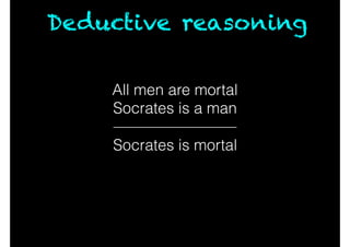
- 14. All men are mortal Socrates is a man Deductive reasoning Socrates is mortal
- 15. All men are mortal Socrates is a man Deductive reasoning Socrates is mortal Idea: Intelligence is deductive reasoning!
- 16. Articles
- 17. Trenchard More, John McCarthy, Marvin Minsky, Oliver Selfridge, Ray Solomonoff 50 years later
- 18. “To understand the real world, we must have a different set of primitives from the relatively simple line trackers suitable and sufficient for the blocks world” — Patrick Winston (1975) Director of MIT’s AI lab from 1972-1997 A bump in the road
- 20. Reductio ad absurdum “Intelligence is 10 million rules” — Doug Lenat
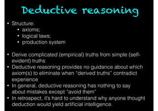
- 21. Deductive reasoning • Structure: • axioms; • logical laws; • production system • Derive complicated (empirical) truths from simple (self- evident) truths • Deductive reasoning provides no guidance about which axiom(s) to eliminate when “derived truths” contradict experience • In general, deductive reasoning has nothing to say about mistakes except “avoid them” • In retrospect, it’s hard to understand why anyone thought deduction would yield artificial intelligence.
- 22. Inductive reasoning “this book is composed […] upon one very simple theme […] that we can learn from our mistakes”
- 23. Inductive reasoning Socrates is mortal Plato is mortal [ … more examples …] All men are mortal
- 24. Inductive reasoning All observed As are Bs a is an A a is a B
- 25. The problem of induction All observed As are Bs a is an A a is a B This is clearly false. The conclusion does not follow from the premises.
- 26. “If a machine is […] infallible, it cannot also be intelligent. There are […] theorems which say almost exactly that. But these theorems say nothing about how much intelligence may be displayed if a machine makes no pretence at infallibility.” [ it’s ok to make mistakes ]
- 27. Let’s look at some examples
- 28. Sequential prediction Scenario: At time t, Forecaster predicts 0 or 1. Nature then reveals the truth. Forecaster has access to N experts. One of them is always correct. Goal: Predict as accurately as possible.
- 29. Halving Algorithm While t>0: Predict by majority vote.Step 1. Remove experts that are wrong.Step 2. t ← t+1Step 3. Set t = 1.
- 30. While t>0: Question: Predict by majority vote.Step 1. Remove experts that are wrong.Step 2. t ← t+1Step 3. How long to find correct expert? Set t = 1. Halving Algorithm
- 31. While t>0: BAD!!! Predict by majority vote.Step 1. Remove experts that are wrong.Step 2. t ← t+1Step 3. How long to find correct expert? Set t = 1. Halving Algorithm
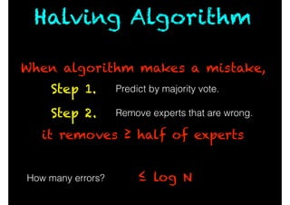
- 32. While t>0: Question: Predict by majority vote.Step 1. Remove experts that are wrong.Step 2. t ← t+1Step 3. How many errors? Set t = 1. Halving Algorithm
- 33. Predict by majority vote.Step 1. Remove experts that are wrong.Step 2. How many errors? Halving Algorithm
- 34. Predict by majority vote.Step 1. Remove experts that are wrong.Step 2. How many errors? When algorithm makes a mistake, it removes ≥ half of experts Halving Algorithm
- 35. ≤ log N Predict by majority vote.Step 1. Remove experts that are wrong.Step 2. How many errors? When algorithm makes a mistake, it removes ≥ half of experts Halving Algorithm
- 36. What’s going on? Didn’t we just use deductive reasoning!?!
- 37. What’s going on? Didn’t we just use deductive reasoning!?! Yes… but No!
- 38. What’s going on? Algorithm: makes educated guesses about Nature Analysis: proves theorem about number of errors (inductive) (deductive)
- 39. What’s going on? Algorithm: makes educated guesses about Nature Analysis: proves theorem about number of errors (inductive) (deductive) The algorithm learns — but it does not deduce!
- 40. Adversarial prediction Scenario: At time t, Forecaster predicts 0 or 1. Nature then reveals the truth. Forecaster has access to N experts. One of them is always correct. Nature is adversarial. Goal: Predict as accurately as possible.
- 41. At time t, Forecaster predicts 0 or 1. Nature then reveals the truth. Forecaster has access to N experts. One of them is always correct. Nature is adversarial. Goal: Predict as accurately as possible. Seriously?!?!
- 42. Regret Let m* be the best expert in hindsight. regret := # mistakes(Forecaster) - # mistakes(m*) Goal: Predict as accurately as possible. Minimize regret.
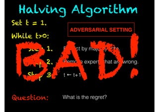
- 43. While t>0: Question: Predict by majority vote.Step 1. Remove experts that are wrong.Step 2. t ← t+1Step 3. What is the regret? Set t = 1. Halving Algorithm ADVERSARIAL SETTING
- 44. While t>0: Question: Predict by majority vote.Step 1. Remove experts that are wrong.Step 2. t ← t+1Step 3. What is the regret? Set t = 1. Halving Algorithm ADVERSARIAL SETTING BAD!
- 45. While t ≤ T: Question: Predict by weighted majority vote.Step 1. Multiply incorrect experts by β.Step 2. t ← t+1Step 3. What is the regret? Set t = 1. Weighted Majority Alg Pick β in (0,1). Assign 1 to experts.
- 46. While t ≤ T: Predict by weighted majority vote.Step 1. Multiply incorrect experts by β.Step 2. t ← t+1Step 3. Set t = 1. What is the regret? [ choose β carefully ] r T · log N 2 Pick β in (0,1). Assign 1 to experts. Weighted Majority Alg
- 47. Loss functions `(y, y0 ) = 1 2 ⇣ y y0 ⌘2 `(p, i) = ( log(1 p) if i = 0 log(p) else `(y, y0 ) = ( 0 if y = y0 1 else • 0/1 loss • Mean square error • Logistic loss
- 48. Loss functions `(y, y0 ) = 1 2 ⇣ y y0 ⌘2 `(p, i) = ( log(1 p) if i = 0 log(p) else `(y, y0 ) = ( 0 if y = y0 1 else • 0/1 loss • Mean square error • Logistic loss not convex convex
- 49. Exp. Weights Alg. While t ≤ T: Predict the weighted sum.Step 1. Multiply expert i byStep 2. t ← t+1Step 3. Set t = 1. What is the regret? [ choose β carefully ] Pick β > 0. Assign 1 to experts. e ·`(ft i ,yt ) log N + p 2T log N
- 50. Inductive reasoning • Structure: • game played over a series of rounds • on each round, experts make predictions • Forecaster takes weighted average of predictions • Nature reveals the truth and a loss is incurred • Forecaster adjusts weights • correct experts —> increase weights; • incorrect —> decrease • Goal: • average loss per round converges to best-in- hindsight
- 51. Inductive reasoning • How it works • Forecaster adjusts strategy according to prior experience • Current strategy encodes previous mistakes • No guarantee on any particular example • Performance is optimal on average • Still to come • How can Forecaster communicate its knowledge with others, in a way that is useful to them?
- 52. Gradient descent “the great watershed in optimisation isn’t between linearity and nonlinearity, but convexity and nonconvexity” — Tyrrell Rockafellar
- 53. Gradient descent • Everyone knows (?) gradient descent • Take a fresh look: • gradient descent is a no-regret algorithm • —> game theory • —> neural networks
- 54. Online Convex Opt. Scenario: Convex set K; differentiable loss L(a,b) that is convex function of a At time t, Forecaster picks at in K Nature responds with bt in K [ Nature is adversarial ] Forecaster’s loss is L(a,b) Goal: Minimize regret. � �� �� �� � � � � � � �� �
- 55. Follow the Leader Idea: Predict the at that would have worked best on { b1, … ,bt-1 }
- 56. While t ≤ T: Step 1. Step 2. Set t = 1. Follow the Leader Idea: t ← t+1 Pick a1 at random. at := argmin a2K "t 1X i=1 L(a, bi) # Predict the at that would have worked best on { b1, … ,bt-1 }
- 57. While t ≤ T: Step 1. Step 2. Set t = 1. Follow the Leader BAD! Problem: Nature pulls Forecaster back-and-forth No memory! t ← t+1 Pick a1 at random. at := argmin a2K "t 1X i=1 L(a, bi) #
- 58. While t ≤ T: Step 1. Step 2. Set t = 1. t ← t+1 FTRL Pick a1 at random. regularize at := argmin a2K "t 1X i=1 L(a, bi) + 2 · kak2 2 #
- 59. While t ≤ T: Step 1. Step 2. Set t = 1. FTRL t ← t+1 Pick a1 at random. gradient descent at at 1 · @ @a L(at 1, bt 1)
- 60. While t ≤ T: Step 1. Step 2. Set t = 1. FTRL Intuition: β controls memory t ← t+1 Pick a1 at random. at at 1 · @ @a L(at 1, bt 1)
- 61. While t ≤ T: Step 1. Step 2. Set t = 1. FTRL What is the regret? [ choose β carefully ] diam(K) · Lipschitz(L) · p T t ← t+1 Pick a1 at random. at at 1 · @ @a L(at 1, bt 1)
- 62. Logarithmic regret regret [ choose β carefully ] Convergence at rate is actually quite slow • For many common loss functions • (e.g. mean-square error, logistic loss) • it is possible to do much better p T T log T T
- 63. Information theory Two connections • Entropic regularization <—> • Exponential Weights Algorithm • Analogy between gradients and Fano information • “the information represented by y about x” log P(x|y) P(x)
- 64. Gradient descent • Gradient descent is fast, cheap, and guaranteed to converge — even against adversaries • “a hammer that smashes convex nails” � �� �� �� � � � � � � �� � • GD is well-understood in convex settings • Convergence rate depends on the structure of the loss, size of search space, etc.
- 65. Convex optimization Convex methods • Stochastic gradient descent • Nesterov momentum • BFGS (Broyden-Fletcher-Goldfarb-Shanno) • Conjugate gradient methods • AdaGrad
- 66. Online Convex Opt. (deep learning) Apply Gradient Descent to nonconvex optimization (neural networks). • Theorems don’t work (not convex) • tons of engineering (decades of tweaking) Amazing performance. Figure 3 | From image to text. Captions generated by a recurrent neural network (RNN) taking, as extra input, the representation extracted by a deep with permission from ref. 102. When the RNN is given the ability to focus attention on a different location in the input image (middle and bottom; th Deep CNN Generating RNN A group of people shopping at an outdoor market. There are many vegetables at the fruit stand. A woman is throwing a frisbee in a park. A little girl sitting on a bed with a teddy bear. A group of people sitting on a boat in the water. A giraffe standing in a forest with trees in the background. A dog is standing on a hardwood floor. A stop sign is on a road with a mountain in the background
- 67. Deep Learning • Superhuman performance on object recognition (ImageNet) • Outperformed humans at recognising street-signs (Google streetview). • Superhuman performance on Atari games (Google). • Real-time translation: English voice to Chinese voice (Microsoft).
- 68. Game theory “An equilibrium is not always an optimum; it might not even be good. This may be the most important discovery of game theory.” — Ivar Ekeland
- 69. Game theory • So far • Seen how Forecaster can learn to use “expert” advice. • Forecaster modifies the weights of experts such that it converges to optimal-in-hindsight predictions. • Who are these experts? • We will model them as Forecasters in their own right • First, let’s develop tools for modeling populations.
- 70. Setup • Players A, B with actions {a1, a2, … am} and {b1, b2, … bn} • Two payoff matrices, describing the losses/gains of the players for every combination of moves • Goal of players is to maximise-gain / minimise-loss • Neither player knows what the other will do
- 71. Setup • Players A, B with actions {a1, a2, … am} and {b1, b2, … bn} • Two payoff matrices, describing the losses/gains of the players for every combination of moves A B R P R P 0 Rock-paper -scissors (zero-sum game) S S 0 0 -1 1 1 -1 -1 1 A B R P R P 0 S S 0 0 1 -1 -1 1 1 -1
- 72. Minimax theorem inf a2K sup b2K L(a, b) = sup b2K inf a2K L(a, b)
- 73. Minimax theorem Forecaster picks a, Nature responds b inf a2K sup b2K L(a, b) = sup b2K inf a2K L(a, b)
- 74. Minimax theorem Forecaster picks a, Nature responds b Nature picks b, Forecaster responds a inf a2K sup b2K L(a, b) = sup b2K inf a2K L(a, b)
- 75. Minimax theorem Forecaster picks a, Nature responds b Nature picks b, Forecaster responds a inf a2K sup b2K L(a, b) = sup b2K inf a2K L(a, b) A B R P R P 0 S S 0 0 -1 1 1 -1 -1 1 A B R P R P 0 S S 0 0 1 -1 -1 1 1 -1
- 76. Minimax theorem Forecaster picks a, Nature responds b Nature picks b, Forecaster responds a inf a2K sup b2K L(a, b) = sup b2K inf a2K L(a, b) inf a2K sup b2K L(a, b) sup b2K inf a2K L(a, b) going first hurts Forecaster, so
- 77. Minimax theorem Proof idea: No-regret algorithm → → → Forecaster can asymptotically match hindsight Order of players doesn’t matter asymptotically Convert series of moves into average via online-to-batch. Let m* be the best move in hindsight. regret := loss(Forecaster) - loss(m*) inf a2K sup b2K L(a, b) sup b2K inf a2K L(a, b)
- 78. Minimax theorem Proof idea: No-regret algorithm → → → Forecaster can asymptotically match hindsight Order of players doesn’t matter asymptotically Convert series of moves into average via online-to-batch. Let m* be the best move in hindsight. regret := loss(Forecaster) - loss(m*) inf a2K sup b2K L(a, b) sup b2K inf a2K L(a, b)
- 79. Minimax theorem Proof idea: No-regret algorithm → → → Forecaster can asymptotically match hindsight Order of players doesn’t matter asymptotically Convert series of moves into average via online-to-batch. Let m* be the best move in hindsight. regret := loss(Forecaster) - loss(m*) inf a2K sup b2K L(a, b) sup b2K inf a2K L(a, b)
- 80. Minimax theorem Proof idea: No-regret algorithm → → → Forecaster can asymptotically match hindsight Order of players doesn’t matter asymptotically Convert series of moves into average via online-to-batch. Let m* be the best move in hindsight. regret := loss(Forecaster) - loss(m*) ¯a = 1 T TX t=1 at inf a2K sup b2K L(a, b) sup b2K inf a2K L(a, b)
- 81. Nash equilibrium Nash equilibrium <—> no player benefits by deviating
- 82. Nash equilibrium Nash equilibrium <—> no player benefits by deviating A B Deny Confess Deny Confess -2/-2 -6/0 0/-6 -6/-6 Prisoner’s dilemma:
- 83. Nash equilibrium Problems: • Computationally hard (PPAD-complete, Daskalakis 2008) • Some outcomes are very bad
- 84. Nash equilibrium A B Stop Go Stop Go 0/0 10/0 0/10 -∞/-∞ Blind-intersection dilemma:
- 85. Nash equilibrium A B Stop Go Stop Go 0/0 10/0 0/10 -∞/-∞ Blind-intersection dilemma: Equilibrium: both drivers STOP; no-one uses intersection
- 86. Correlated equilibrium A B Stop Go Stop Go 0/0 10/0 0/10 -∞/-∞ Traffic light: P(x, y) = 8 >< >: 1 2 if x = S and y = G 1 2 if x = G and y = S 0 else Blind-intersection dilemma:
- 87. Correlated equilibrium A B Stop Go Stop Go 0/0 10/0 0/10 -∞/-∞ Blind-intersection dilemma: • Better outcomes for players: Correlated equilibria can be much better than Nash equilibria (depending on the signal)
- 88. Convex games • Players with convex action sets • Loss functions where and each loss is separately convex in each argument • Players aim to minimize their losses • Player do not know what other players will do `i(w1, . . . , wN) {Pi}N i=1 {Ki}N i=1 wi 2 Ki
- 89. Sketch of proof: Since player j applies a no-regret algorithm, it follows that after T rounds, its sequence of moves {wt j} has a loss within of the optimal, wj *. Interpreting the historical sequence of plays as a signal obtains The result follows by letting —> 0. No-regret —> Corr. eqm 1 T X `i(wt j , wt j) `i(w⇤ j , wt j) ✏ 8w⇤ j ✏ ✏ E h `(w) i E h `(w⇤ j , w j) i + ✏
- 90. Nash —> Aumann From Nash equilibrium to correlated equilibrium: • Computationally tractable: No-regret algorithms converge on coarse correlated equilibria • Better outcomes: Signal is the past actions of players, chosen according to an optimal strategy
- 91. • Every game has a Nash equilibrium • Economists typically assume that economy is in Nash equilibrium • But Nash equilibria are hard to find and are often unpleasant • Correlated equilibria are easier to compute and can be better for the players • A signal is required to coordinate players: • set signally externally • e.g. traffic light • in repeated games, construct signal as the average of historical behavior • e.g. no-regret learning Game theory
- 92. • Correlated equilibrium • Players converge on mutually agreeable outcomes by adapting to each other’s behavior over repeated rounds • The signal provides a “strong hint” about where to find equilibria. • Nash equilibrium • It’s hard to guess what others will do when playing de novo (intractability); and • You haven’t established a track record to build on (undesirability) Game theory
- 93. Gradients and Games Gradient descent is a no-regret algorithm • Insert players using gradient descent into any convex game, and they will converge on a correlated equilibrium • Global convergence to correlated equilibrium is controlled by convergence of players to their best-in-hindsight local optimum Next: • Gradient descent + chain rule = backprop
- 94. Neural networks “Anything a human can do in a fraction of a second, a deep network can do too” — Ilya Sutskever
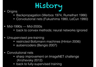
- 95. • Origins • Backpropagation (Werbos 1974, Rumelhart 1986) • Convolutional nets (Fukushima 1980, LeCun 1990) • Mid-1990s — Mid-2000s • back to convex methods; neural networks ignored • Unsupervised pre-training • restricted Boltzmann machines (Hinton 2006) • autoencoders (Bengio 2007) • Convolutional nets • sharp improvement on ImageNET challenge (Krizhevsky 2012) • back to fully-supervised training History
- 96. • Convolutional nets • sharp improvement on ImageNET challenge (Krizhevsky 2012) • back to fully-supervised training History
- 97. 30 years of trial-and-error • Architecture • Weight-tying (convolutions) • Max-pooling • Nonlinearity • Rectilinear units (Jarrett 2009) • Credit assignment • Backpropagation • Optimization • Stochastic Gradient Descent • Nesterov momentum, BFGS, AdaGrad, etc. • RMSProp (Riedmiller 1993, Hinton & Tieleman 200x) • Regularization • Dropout (Srivastava et al 2014) or • Batch-Normalization (Szegedy & Ioffe 2015)
- 98. Why (these) NNs? • Why neural networks? • GPUs • Good local minima (no-one knows why) • “Mirrors the world’s compositional structure” • Why ReLUs, Why Max-Pooling, Why convex methods? • “locally” convex optimization (this talk)
- 99. Neural networks Input Layer1 W1 Matrix mult Layer2 W2 Matrix mult Output W3 Matrix mult Nonlinearity Nonlinearity fW(x)
- 100. Neural networks Input Layer1 W1 Matrix mult Layer2 W2 Matrix mult Output W3 Matrix mult Nonlinearity Nonlinearity `(fW(x), y) label loss
- 101. Univ Function Approx Theorem (Leshno 1993): A two-layer neural network with infinite width and nonpolynomial nonlinearity is dense in the space of continuous functions. � ��� �� � � �� ���� ���� ��� ��� ��� � � ��� �� � � �� ���� ���� ��� ��� ��� � Sigmoid Tanh (x) = 1 1 + e x ⌧(x) = ex e x ex + e x � ��� �� � � �� ���� ���� ��� ��� ��� � ReLU ⇢(x) = max(0, x)
- 102. � ��� �� � � �� ���� ���� ��� ��� ��� � � ��� �� � � �� ���� ���� ��� ��� ��� � � ��� �� � � �� ���� ���� ��� ��� ��� � d⇢ dx d dx d⌧ dx � ��� �� � � �� ���� ���� ��� ��� ��� � � ��� �� � � �� ���� ���� ��� ��� ��� � � ��� �� � � �� ���� ���� ��� ��� ��� � ⌧⇢
- 103. The chain rule h g f df dx = df dg · dg dh · dh dx f g h(x) = f(g(h(x)))
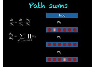
- 106. Input W1 W2 W3 Weight updates j Gradient descent Wt+1 ij Wt ij ⌘ · @` @Wij
- 107. Input W1 W2 W3 Weight updates j Gradient descent Wt+1 ij Wt ij ⌘ · @` @Wij by the chain rule @` @Wij = @` @xj · @xj @Wij
- 108. Input W1 W2 W3 Weight updates j Gradient descent Wt+1 ij Wt ij ⌘ · @` @Wij by the chain rule since @xj @Wij = xi @` @Wij = @` @xj · xi
- 109. Input W1 W2 W3 Weight updates j Gradient descent Wt+1 ij Wt ij ⌘ · @` @Wij by the chain rule also, define j := @` @xj @` @Wij = j · xi
- 110. Input W1 W2 W3 Weight updates j Gradient descent Wt+1 ij Wt ij ⌘ · @` @Wij by the chain rule How to compute? j := @` @xj @` @Wij = j · xi
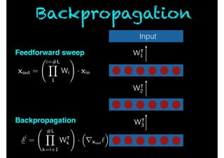
- 111. Input i = #LY k=i+1 W| k ! · ⇣ rxout ` ⌘ xout = i=#LY 1 Wi ! · xin W| 1 W| 2 W| 3 Feedforward sweep Backpropagation Backpropagation
- 112. Max-pooling Pick element with max output in each block; zero out the rest
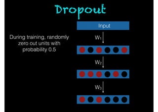
- 113. Dropout Input W1 W2 W3 During training, randomly zero out units with probability 0.5
- 114. ReLU networks Input W1 W2 W3 � ��� �� � � �� ���� ���� ��� ��� ��� � ReLU ⇢(x) = max(0, x)
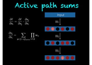
- 117. Active path sums Input W1 W2 W3 i j @` @xi = @` @xj · @xj @xi @xj @xi = X p2{i!j}active Y ↵2p w↵
- 118. Knowledge distribution • Units in NN <—> Players in a game • All units have the same loss • Loss is convex function of units’ weights when unit is active • Units in output layer compute error-gradients • Other units distribute signals of the form (error-gradients) x (path-sums)
- 119. Circadian games • Units have convex losses when active • Neural networks are circadian games • i.e. game that is convex for active (awake) players Main Theorem. Convergence of neural network to correlated equilibrium is upper-bounded by convergence rates of individual units. Corollary. Units perform convex optimization when active. Convex methods and guarantees (on convergence rates) apply to neural networks. —> Explains why ReLUs work so well.
- 120. Philosophical Corollary • Neural networks are games Units are no-regret learners • Unlike many games (e.g. in micro-economic theory), the equilibria in NNs are extremely desirable • Error-backpropagation distributes gradient- information across units • Claim: There is a theory of distributed reasoning implicit in gradient descent and the chain rule.
- 121. The End. Questions?