SlideShare a Scribd company logo
Prof. Vijay M. Shekhat
9558045778
vijay.shekhat@darshan.ac.in
2160703
Computer Graphics
Unit-2
Graphics Primitives
Unit: 2 Graphics Primitives 2
Unit: 2 Graphics Primitives 2 Darshan Institute of Engineering & Technology
Darshan Institute of Engineering & Technology
Outline
 Points
 Line drawing algorithms.
 Circle drawing algorithm.
 Ellipse drawing algorithm.
 Scan-Line polygon filling algorithm.
 Inside-Outside test.
 Boundary fill algorithm.
 Flood fill algorithm.
 Character generation.
 Line attributes.
 Color and grayscale levels
 Area fill attributes.
 Character attributes.
Unit: 2 Graphics Primitives 3
Unit: 2 Graphics Primitives 3 Darshan Institute of Engineering & Technology
Darshan Institute of Engineering & Technology
Point
 Point plotting is done by converting a single coordinate position
furnished by an application program into appropriate operations for the
output device in use.
 Example: Plot point
 Line
 Line
 Point
 To draw the point on the screen we use function

 To draw the pixel in C language we use function

 Similarly for retrieving color of pixel we have function

0
1
2
3
4
5
6
7
0 1 2 3 4 5 6 7
Unit: 2 Graphics Primitives 4
Unit: 2 Graphics Primitives 4 Darshan Institute of Engineering & Technology
Darshan Institute of Engineering & Technology
0
1
2
3
4
5
1 2 3 4
Line
 Line drawing is done by calculating intermediate positions along
the line path between two specified endpoint positions.
 The output device is then directed to fill in those positions
between the end points with some color.
 For some device such as a pen plotter or random scan display, a
straight line can be drawn smoothly from one end point to other.
 Digital devices display a straight line segment by plotting discrete
points between the two endpoints.
 Discrete coordinate positions along the line path are calculated
from the equation of the line.
0
1
2
3
4
5
0 2 4 6
Unit: 2 Graphics Primitives 5
Unit: 2 Graphics Primitives 5 Darshan Institute of Engineering & Technology
Darshan Institute of Engineering & Technology
Contd.
 Screen locations are referenced with integer values.
 So plotted positions may only approximate actual line positions
between two specified endpoints. For example line position of
(12.36, 23.87) would be converted to pixel position (12, 24).
 This rounding of coordinate values to integers causes lines to be
displayed with a stair step appearance (“the Jaggies”).
Unit: 2 Graphics Primitives 6
Unit: 2 Graphics Primitives 6 Darshan Institute of Engineering & Technology
Darshan Institute of Engineering & Technology
Line Drawing Algorithms
 The Cartesian slop-intercept equation for a straight line is
•
• with ‘ ’ representing slop and ‘ ’ as the intercept.
 It is possible to draw line using this equation but for efficiency
purpose we use different line drawing algorithm.
• DDA Algorithm
• Bresenham’s Line Algorithm
 We can also use this algorithm in parallel if we have more number
of processors.
Unit: 2 Graphics Primitives 7
Unit: 2 Graphics Primitives 7 Darshan Institute of Engineering & Technology
Darshan Institute of Engineering & Technology
Introduction to DDA Algorithm
 Full form of DDA is Digital Differential Analyzer
 DDA is scan conversion line drawing algorithm based on
calculating either or using line equation.
 We sample the line at unit intervals in one coordinate and find
corresponding integer values nearest the line path for the other
coordinate.
 Selecting unit interval in either or direction based on way we
process line.
Unit: 2 Graphics Primitives 8
Unit: 2 Graphics Primitives 8 Darshan Institute of Engineering & Technology
Darshan Institute of Engineering & Technology
Unit Step Direction in DDA
Algorithm
 Processing from left to right.
 Slope is “+ve”, & Magnitude is Less than 1
 Slope is “-ve”, & Magnitude is Less than 1
 Slope is “+ve”, & Magnitude is greater than 1
 Slope is “-ve”, & Magnitude is greater than 1
 Processing from right to left.
 Slope is “+ve”, & Magnitude is Less than 1
 Slope is “-ve”, & Magnitude is Less than 1
 Slope is “+ve”, & Magnitude is greater than 1
 Slope is “-ve”, & Magnitude is greater than 1
Unit: 2 Graphics Primitives 9
Unit: 2 Graphics Primitives 9 Darshan Institute of Engineering & Technology
Darshan Institute of Engineering & Technology
Derivation of DDA Algorithm
 We sample at unit interval and calculate each successive
value as follow:

 [For first intermediate point]
 [For 𝑡ℎ intermediate point]
 Subtract from


 Using this equation computation becomes faster than normal line
equation.
 As is any real value calculated value must be rounded to nearest
integer.
Unit: 2 Graphics Primitives 10
Unit: 2 Graphics Primitives 10 Darshan Institute of Engineering & Technology
Darshan Institute of Engineering & Technology
Contd.
 We sample at unit interval and calculate each successive
value as follow:

 [For first intermediate point]
 [For 𝑡ℎ intermediate point]
 [For intermediate point]
Subtract from


Similarly
 for ∆x = -1: we obtain
 for ∆y = -1: we obtain
Procedure for DDA line algorithm.
Void lineDDA (int xa, int ya, int xb, int yb)
{
int dx = xb – xa, dy = yb – ya, steps, k;
float xincrement, yincrement, x = xa, y = ya;
if (abs(dx)>abs(dy))
{
Steps = abs (dx);
}
else
{
Steps = abs (dy);
}
xincrement = dx/(float) steps;
yincrement = dy/(float) steps;
setpixel (ROUND (x), ROUND (y));
for(k=0;k<steps;k++)
{
x += xincrement;
y += yincrement;
setpixel (ROUND (x), ROUND (y));
}
}
Unit: 2 Graphics Primitives 12
Unit: 2 Graphics Primitives 12 Darshan Institute of Engineering & Technology
Darshan Institute of Engineering & Technology
Example DDA Algorithm
 Example: Draw line with coordinates , .

 is “+ve” and less than 1 so .
 ,
[Plot the initial point as given]
 ,
[Plot the first intermediate point by rounding it to ]
 ,
[Plot the second intermediate point by rounding it to ]
 ,
[Plot the third intermediate point by rounding it to ]
 ,
[Plot End point given]
0 1 2 3 4 5 6 7 8
4
3
2
1
0
Unit: 2 Graphics Primitives 13
Unit: 2 Graphics Primitives 13 Darshan Institute of Engineering & Technology
Darshan Institute of Engineering & Technology
Introduction to Bresenham’s Line
Algorithm
 An accurate and efficient raster line-generating algorithm,
developed by Bresenham.
 It scan converts line using only incremental integer calculations.
 That can be modified to display circles and other curves.
 Based on slop we take unit step in one direction and decide pixel
of other direction from two candidate pixel.
 If we sample at unit interval and vice versa.
Unit: 2 Graphics Primitives 14
Unit: 2 Graphics Primitives 14 Darshan Institute of Engineering & Technology
Darshan Institute of Engineering & Technology
Line Path & Candidate pixel
 Example |ΔX| > |ΔY|, and ΔY is “+ve”.
 Initial point (Xk, Yk)
 Line path
 Candidate pixels {(Xk+1, Yk), (Xk+1, Yk+1)}
0 1 2 3 4
4
3
2
1
0
 Now we need to decide which candidate pixel is more closer to
actual line.
 For that we use decision parameter (Pk) equation.
 Decision parameter can be derived by calculating distance of
actual line from two candidate pixel.
Unit: 2 Graphics Primitives 15
Unit: 2 Graphics Primitives 15 Darshan Institute of Engineering & Technology
Darshan Institute of Engineering & Technology
Derivation Bresenham’s Line
Algorithm
 [Line Equation]
 [Actual Y value at Xk position]
 [Actual Y value at Xk +1position]
Distance between actual line position and lower candidate
pixel


Distance between actual line position and upper
candidate pixel


0 1 2 3 4
4
3
2
1
0
Unit: 2 Graphics Primitives 16
Unit: 2 Graphics Primitives 16 Darshan Institute of Engineering & Technology
Darshan Institute of Engineering & Technology
Contd.
Calculate



 [Put ]
Decision parameter



 [Replacing single constant C for simplicity]
Similarly

Unit: 2 Graphics Primitives 17
Unit: 2 Graphics Primitives 17 Darshan Institute of Engineering & Technology
Darshan Institute of Engineering & Technology
Contd.
Subtract from


[where ]

[where depending on selection of previous pixel]
Unit: 2 Graphics Primitives 18
Unit: 2 Graphics Primitives 18 Darshan Institute of Engineering & Technology
Darshan Institute of Engineering & Technology
Initial Decision parameter
 The first decision parameter is calculated using equation of .

 [Put ]

[Substitute 0 0]

[Substitute ]


[Initial decision parameter with all terms are constant]
Unit: 2 Graphics Primitives 19
Unit: 2 Graphics Primitives 19 Darshan Institute of Engineering & Technology
Darshan Institute of Engineering & Technology
Bresenham’s Line Algorithm
1. Input the two line endpoints and store the left endpoint in .
2. Load into the frame buffer; that is, plot the first point.
3. Calculate constants , , , and , and obtain the
starting value for the decision parameter as
4. At each along the line, starting at , perform the following test:
If , the next point to plot is and
Otherwise, the next point to plot is and
5. Repeat step-4 times.
Unit: 2 Graphics Primitives 20
Unit: 2 Graphics Primitives 20 Darshan Institute of Engineering & Technology
Darshan Institute of Engineering & Technology
Discryption of Bresenham’s Line
Algorithm
 Bresenham’s algorithm is generalized to lines with arbitrary slope.
 For lines with positive slope greater than 1 we interchange the roles of
the and directions.
 Also we can revise algorithm to draw line from right endpoint to left
endpoint, both and decrease as we step from right to left.
 When 𝑘 we can choose either lower or upper pixel but same for
whole line.
 For the negative slope the procedure are similar except that now one
coordinate decreases as the other increases.
 The special case handle separately by loading directly into the frame
buffer without processing.
 Horizontal line ,
 Vertical line
 Diagonal line with
Unit: 2 Graphics Primitives 21
Unit: 2 Graphics Primitives 21 Darshan Institute of Engineering & Technology
Darshan Institute of Engineering & Technology
Example Bresenham’s Line
Algorithm
 Example: Draw line with coordinates , .
 Plot left end point .
 Calculate:
• ,
• ,
• ,
• ,

 Now so we select upper pixel .

 Now so we select lower pixel .

 Now so we select upper pixel .

 Now so we select lower pixel .
0 1 2 3 4 5 6 7 8
4
3
2
1
0
Unit: 2 Graphics Primitives 22
Unit: 2 Graphics Primitives 22 Darshan Institute of Engineering & Technology
Darshan Institute of Engineering & Technology
Parallel Execution of Line
Algorithms
 The line-generating algorithms we have discussed so far
determine pixel positions sequentially.
 With multiple processors we can calculate pixel position along a
line path simultaneously.
 One way to use multiple processors is partitioning existing
sequential algorithm into small parts and compute separately.
 Alternatively we can setup the processing so that pixel positions
can be calculated efficiently in parallel.
 Balance the load among the available processors is also important
in parallel processing.
Unit: 2 Graphics Primitives 23
Unit: 2 Graphics Primitives 23 Darshan Institute of Engineering & Technology
Darshan Institute of Engineering & Technology
Parallel Bresenham Line
Algorithms
 For number of processors we can set up parallel Bresenham
line algorithm by subdividing the line path into partitions and
simultaneously generating line segment in each of the
subintervals.
 For a line with slope and left endpoint coordinate
position , we partition the line along the positive
direction.
 The distance between beginning positions of adjacent partitions
can be calculated as:
 Where is the width of the line and value for partition with
is computed using integer division.
Unit: 2 Graphics Primitives 24
Unit: 2 Graphics Primitives 24 Darshan Institute of Engineering & Technology
Darshan Institute of Engineering & Technology
Contd.
 Numbering the partitions and the processors, as 0, 1, 2, up to
, we calculate the starting coordinate for the partition
as:
 The change in the direction over each partition is calculated
from the line slope and partition width :
 At the partition, the starting y coordinate is then
Unit: 2 Graphics Primitives 25
Unit: 2 Graphics Primitives 25 Darshan Institute of Engineering & Technology
Darshan Institute of Engineering & Technology
IDP for Parallel Bresenham Line
Algorithms
 The initial decision parameter(IDP) for Bresenham's algorithm at
the start of the subinterval is obtained as follow:


∆
∆


 Each processor then calculates pixel positions over its assigned
subinterval.
Unit: 2 Graphics Primitives 26
Unit: 2 Graphics Primitives 26 Darshan Institute of Engineering & Technology
Darshan Institute of Engineering & Technology
Other Ways for Parallel Execution of Line
Algorithms
 For line with slope greater than 1 we partitioning the line in the
direction and calculating beginning values for the positions.
 For negative slopes, we increment coordinate values in one
direction and decrement in the other.
 Another way to set up parallel algorithms on raster system is to
assign each processor to a particular group of screen pixels.
 With sufficient number of processor we can assign each processor
to one pixel within some screen region.
 This can be done by assigning one processor to each of the pixels
within the limit of the bounding rectangle.
Unit: 2 Graphics Primitives 27
Unit: 2 Graphics Primitives 27 Darshan Institute of Engineering & Technology
Darshan Institute of Engineering & Technology
Contd.
 Perpendicular distance d from line to a particular pixel is
calculated by:

Where



With

 , , and are constant we need to compute only once.
Unit: 2 Graphics Primitives 28
Unit: 2 Graphics Primitives 28 Darshan Institute of Engineering & Technology
Darshan Institute of Engineering & Technology
Contd.
 For the line each processors need to perform two multiplications
and two additions to compute the pixel distance .
 A pixel is plotted if is less than a specified line thickness
parameter.
 Instead of partitioning the screen into single pixels, we can assign
to each processor either a scan line or a column.
 Each processor calculates line intersection with horizontal row or
vertical column of pixels assigned to that processor.
Unit: 2 Graphics Primitives 29
Unit: 2 Graphics Primitives 29 Darshan Institute of Engineering & Technology
Darshan Institute of Engineering & Technology
Contd.
 If vertical column is assign to processor then is fix and it will
calculate .
 Similarly if horizontal row is assign to processor then is fix and
will be calculated.
 Such direct methods are slow in sequential machine but we can
perform very efficiently using multiple processors.
Unit: 2 Graphics Primitives 30
Unit: 2 Graphics Primitives 30 Darshan Institute of Engineering & Technology
Darshan Institute of Engineering & Technology
Circle
 A circle is defined as the set of points that are all at a given
distance from a center position say .
Center
r
Radius
Unit: 2 Graphics Primitives 31
Unit: 2 Graphics Primitives 31 Darshan Institute of Engineering & Technology
Darshan Institute of Engineering & Technology
Properties of Circle- Cartesion
Coordinate
 Cartesian coordinates equation :

 We could use this equation to calculate circular boundary points.
 We increment 1 in direction in every steps from to
and calculate corresponding values at each position as:




Unit: 2 Graphics Primitives 32
Unit: 2 Graphics Primitives 32 Darshan Institute of Engineering & Technology
Darshan Institute of Engineering & Technology
Contd.
 But this is not best method as it requires more number of
calculations which take more time to execute.
 And also spacing between the plotted pixel positions is not
uniform.
 We can adjust spacing by stepping through y values and
calculating x values whenever the absolute value of the slop of the
circle is greater than 1.
 But it will increases computation time.
Unit: 2 Graphics Primitives 33
Unit: 2 Graphics Primitives 33 Darshan Institute of Engineering & Technology
Darshan Institute of Engineering & Technology
Properties of Circle- Polar
Coordinate
 Another way to eliminate the non-uniform spacing is to draw circle
using polar coordinates ‘r’ and ‘’.
 Calculating circle boundary using polar equation is given by pair of
equations which is as follows.


 When display is produce using these equations using fixed angular
step size circle is plotted with uniform spacing.
 The step size ‘’ is chosen according to application and display
device.
 For a more continuous boundary on a raster display we can set the
step size at .
Unit: 2 Graphics Primitives 34
Unit: 2 Graphics Primitives 34 Darshan Institute of Engineering & Technology
Darshan Institute of Engineering & Technology
Properties of Circle- Symmetry
 Computation can be reduced by considering symmetry city
property of circles.
 The shape of circle is similar in each octant.
𝑂
(X, Y)
(Y, X)
(X, -Y)
(Y, -X)
(-X, -Y)
(-Y, -X)
(-Y, X)
(-X, Y)
(4, 3)
(3, 4)
(4, -3)
(3, -4)
(-4, -3)
(-3, -4)
(-3, 4)
(-4, 3)
Unit: 2 Graphics Primitives 35
Unit: 2 Graphics Primitives 35 Darshan Institute of Engineering & Technology
Darshan Institute of Engineering & Technology
Circle Algorithm
 Taking advantage of this symmetry property of circle we can
generate all pixel position on boundary of circle by calculating only
one sector from to .
 Determining pixel position along circumference of circle using any
of two equations shown above still required large computation.
 More efficient circle algorithm are based on incremental
calculation of decision parameters, as in the Bresenham line
algorithm.
 Bresenham’s line algorithm can be adapted to circle generation by
setting decision parameter for finding closest pixel to the
circumference at each sampling step.
Unit: 2 Graphics Primitives 36
Unit: 2 Graphics Primitives 36 Darshan Institute of Engineering & Technology
Darshan Institute of Engineering & Technology
Contd.
 A method for direct distance comparison to test the midpoint
between two pixels to determine if this midpoint is inside or
outside the circle boundary.
 This method is easily applied to other conics also.
 Midpoint approach generates same pixel position as generated by
bresenham’s circle algorithm.
 The error involve in locating pixel positions along any conic section
using midpoint test is limited to one-half the pixel separation.
Unit: 2 Graphics Primitives 37
Unit: 2 Graphics Primitives 37 Darshan Institute of Engineering & Technology
Darshan Institute of Engineering & Technology
Introduction to Midpoint Circle
Algorithm
 In this we sample at unit interval and determine the closest pixel
position to the specified circle path at each step.
 Given radius and center
 We first setup our algorithm to calculate circular path coordinates
for center .
 And then we will transfer calculated pixel position to center
by adding to and to .
 Along the circle section from to in the first quadrant,
the slope of the curve varies from to .
 So we can step unit step in positive direction over this octant
and use a decision parameter to determine which of the two
possible position is closer to the circular path.
Unit: 2 Graphics Primitives 38
Unit: 2 Graphics Primitives 38 Darshan Institute of Engineering & Technology
Darshan Institute of Engineering & Technology
Decision Parameter Midpoint Circle
Algorithm
 Position in the other seven octants are then obtain by symmetry.
 For the decision parameter we use the circle function which is:
 Above equation we calculate for the mid positions between pixels
near the circular path at each sampling step.
 And we setup incremental calculation for this function as we did in
the line algorithm.
Unit: 2 Graphics Primitives 39
Unit: 2 Graphics Primitives 39 Darshan Institute of Engineering & Technology
Darshan Institute of Engineering & Technology
Midpoint between Candidate
pixel
 Figure shows the midpoint between the two candidate pixels at
sampling position .
 Assuming we have just plotted the pixel at
 Next we determine whether the pixel at position or
the one at position is closer to circle boundary.
Midpoint
Candidate
Pixel
Unit: 2 Graphics Primitives 40
Unit: 2 Graphics Primitives 40 Darshan Institute of Engineering & Technology
Darshan Institute of Engineering & Technology
Derivation Midpoint Circle
Algorithm
 So for finding which pixel is more closer using decision parameter
evaluated at the midpoint between two candidate pixels as below:


 If , midpoint is inside the circle and the pixel on the scan
line is closer to circle boundary.
 Otherwise midpoint is outside or on the boundary and we select
the scan line .
Unit: 2 Graphics Primitives 41
Unit: 2 Graphics Primitives 41 Darshan Institute of Engineering & Technology
Darshan Institute of Engineering & Technology
Contd.
 Successive decision parameters are obtain using incremental
calculations as follows:


 Now we can obtain recursive calculation using equation of and
as follow


Unit: 2 Graphics Primitives 42
Unit: 2 Graphics Primitives 42 Darshan Institute of Engineering & Technology
Darshan Institute of Engineering & Technology
Contd.




 Now we can put

Unit: 2 Graphics Primitives 43
Unit: 2 Graphics Primitives 43 Darshan Institute of Engineering & Technology
Darshan Institute of Engineering & Technology
Contd.

 In above equation is either or depending on the
sign of the .
 If we select .

 If we select .




Unit: 2 Graphics Primitives 44
Unit: 2 Graphics Primitives 44 Darshan Institute of Engineering & Technology
Darshan Institute of Engineering & Technology
Contd.


 Now put .

Unit: 2 Graphics Primitives 45
Unit: 2 Graphics Primitives 45 Darshan Institute of Engineering & Technology
Darshan Institute of Engineering & Technology
IDP Midpoint Circle Algorithm
 The initial decision parameter(IDP) is obtained by evaluating the
circle function at the start position as follows.





Algorithm for Midpoint Circle Generation
1. Input radius r and circle center , and obtain the first point on the
circumference of a circle centered on the origin as
2. calculate the initial value of the decision parameter as
3. At each position, starting at , perform the following test:
If , the next point along the circle centered on is
Otherwise, the next point along the circle is
Where , & .
4. Determine symmetry points in the other seven octants.
5. Move each calculated pixel position onto the circular path centered on
and plot the coordinate values:
,
6. Repeat steps 3 through 5 until .
Unit: 2 Graphics Primitives 47
Unit: 2 Graphics Primitives 47 Darshan Institute of Engineering & Technology
Darshan Institute of Engineering & Technology
 Example: Draw circle with radius , and center of circle is
(Only one octant to )
 First we find pixel position for octant to for center


 Now we select (1, 10)


 Now we select (2, 10)
Example Midpoint Circle
Algorithm
𝒌 𝟏 𝒌 𝟏
𝒌
(1, 10)
-9
0
(2, 10)
-6
1
(3, 10)
-1
2
(4, 9)
6
3
(5, 9)
-3
4
(6, 8)
8
5
(7, 7)
5
6
Unit: 2 Graphics Primitives 48
Unit: 2 Graphics Primitives 48 Darshan Institute of Engineering & Technology
Darshan Institute of Engineering & Technology


 Now we select (3, 10)


 Now we select (4, 9)


 Now we select (5, 9)
Contd.
𝒌 𝟏 𝒌 𝟏
𝒌
(1, 10)
-9
0
(2, 10)
-6
1
(3, 10)
-1
2
(4, 9)
6
3
(5, 9)
-3
4
(6, 8)
8
5
(7, 7)
5
6
Unit: 2 Graphics Primitives 49
Unit: 2 Graphics Primitives 49 Darshan Institute of Engineering & Technology
Darshan Institute of Engineering & Technology


 Now we select (6, 8)


 Now we select (7, 7)
 Now Loop exit as , as
 in our case
Contd.
𝒌 𝟏 𝒌 𝟏
𝒌
(1, 10)
-9
0
(2, 10)
-6
1
(3, 10)
-1
2
(4, 9)
6
3
(5, 9)
-3
4
(6, 8)
8
5
(7, 7)
5
6
Unit: 2 Graphics Primitives 50
Unit: 2 Graphics Primitives 50 Darshan Institute of Engineering & Technology
Darshan Institute of Engineering & Technology
Contd.
 Than we calculate pixel position for given center using
equations:


Center (1, 1)
Center (0, 0)
(2, 11)
(1, 10)
(3, 11)
(2, 10)
(4, 11)
(3, 10)
(5, 10)
(4, 9)
(6, 10)
(5, 9)
(7, 9)
(6, 8)
(8, 8)
(7, 7)
Unit: 2 Graphics Primitives 51
Unit: 2 Graphics Primitives 51 Darshan Institute of Engineering & Technology
Darshan Institute of Engineering & Technology
Contd.
 Plot the pixel.
 First plot initial point.
(1, 11)
Center (1, 1)
(2, 11)
(3, 11)
(4, 11)
(5, 10)
(6, 10)
(7, 9)
(8, 8)
12
11
10
9
8
7
6
5
4
3
2
1
0
0 1 2 3 4 5 6 7 8 9 10 11
Center
(1, 1)
Unit: 2 Graphics Primitives 52
Unit: 2 Graphics Primitives 52 Darshan Institute of Engineering & Technology
Darshan Institute of Engineering & Technology
Ellipse
 AN ellipse is defined as the set of points such that the sum of the
distances from two fixed positions (foci) is same for all points.
Unit: 2 Graphics Primitives 53
Unit: 2 Graphics Primitives 53 Darshan Institute of Engineering & Technology
Darshan Institute of Engineering & Technology
Contd.
 If we labeled distance from two foci to any point on ellipse
boundary as and then the general equation of an ellipse can
be written as:
 Expressing distance in terms of focal coordinates and
we have

[Using Distance formula]
Unit: 2 Graphics Primitives 54
Unit: 2 Graphics Primitives 54 Darshan Institute of Engineering & Technology
Darshan Institute of Engineering & Technology
Properties of Ellipse-Specifying
Equations
 An interactive method for specifying an ellipse in an arbitrary
orientation is to input
 two foci and
 a point on the ellipse boundary.
 With this three coordinates we can evaluate constant in equation:
 We can also write this equation in the form
 Where the coefficients , and are evaluated in terms
of the focal coordinates and the dimensions of the major and
minor axes of the ellipse.
Unit: 2 Graphics Primitives 55
Unit: 2 Graphics Primitives 55 Darshan Institute of Engineering & Technology
Darshan Institute of Engineering & Technology
Contd.
 Then coefficient in can be
evaluated and used to generate pixels along the elliptical path.
 We can say ellipse is in standard position if their major and minor
axes are parallel to x-axis and y-axis.
 Ellipse equation are greatly simplified if we align major and minor
axis with coordinate axes i.e. x-axis and y-axis.
X-axis
Y-axis
Unit: 2 Graphics Primitives 56
Unit: 2 Graphics Primitives 56 Darshan Institute of Engineering & Technology
Darshan Institute of Engineering & Technology
Contd.
 Equation of ellipse can be written in terms of the ellipse center
coordinates and parameters and as.
 Using the polar coordinates r and θ, we can also describe the
ellipse in standard position with the parametric equations:
Unit: 2 Graphics Primitives 57
Unit: 2 Graphics Primitives 57 Darshan Institute of Engineering & Technology
Darshan Institute of Engineering & Technology
 Symmetry property further reduced computations.
 An ellipse in standard position is symmetric between quadrant.
Properties of Ellipse-Symmetry
Unit: 2 Graphics Primitives 58
Unit: 2 Graphics Primitives 58 Darshan Institute of Engineering & Technology
Darshan Institute of Engineering & Technology
Introduction to Midpoint Ellipse
Algorithm
 Given parameters .
 We determine points for an ellipse in standard position
centered on the origin.
 Then we shift the points so the ellipse is centered at .
 If we want to display the ellipse in nonstandard position then we
rotate the ellipse about its center to align with required direction.
 For the present we consider only the standard position.
 We draw ellipse in first quadrant and than use symmetry property
for other three quadrant.
Unit: 2 Graphics Primitives 59
Unit: 2 Graphics Primitives 59 Darshan Institute of Engineering & Technology
Darshan Institute of Engineering & Technology
 In this method we divide first quadrant into two parts according to
the slope of an ellipse
 Boundary divides region at
• slope = -1.
 We take unit step in X direction
• If magnitude of ellipse slope < 1 (Region 1).
 We take unit step in Y direction
• If magnitude of ellipse slope > 1 (Region 2).
Regions in Midpoint Ellipse
Algorithm
Region 1
Region 2
Unit: 2 Graphics Primitives 60
Unit: 2 Graphics Primitives 60 Darshan Institute of Engineering & Technology
Darshan Institute of Engineering & Technology
Ways of Processing Midpoint Ellipse
Algorithm
 We can start from and step clockwise along the elliptical
path in the first quadrant
 Alternatively, we could start at and select points in a
counterclockwise order.
 With parallel processors, we could calculate pixel positions in the
two regions simultaneously.
 Here we consider sequential implementation of midpoint
algorithm.
 We take the start position at and steps along the elliptical
path in clockwise order through the first quadrant.
Unit: 2 Graphics Primitives 61
Unit: 2 Graphics Primitives 61 Darshan Institute of Engineering & Technology
Darshan Institute of Engineering & Technology
Decision Parameter Midpoint Ellipse
Algorithm
 We define ellipse function for center of ellipse at (0, 0) as follows.

 Which has the following properties:
 Thus the ellipse function serves as the decision parameter in the
midpoint ellipse algorithm.
 At each sampling position we select the next pixel from two
candidate pixel.
Unit: 2 Graphics Primitives 62
Unit: 2 Graphics Primitives 62 Darshan Institute of Engineering & Technology
Darshan Institute of Engineering & Technology
Processing Steps of Midpoint Ellipse
Algorithm
 Starting at we take unit step in direction until we reach
the boundary between region-1 and region-2.
 Then we switch to unit steps in direction in remaining portion on
ellipse in first quadrant.
Region 1
Region 2
 At each step we need to test the value
of the slope of the curve for deciding
the end point of the region-1.
Unit: 2 Graphics Primitives 63
Unit: 2 Graphics Primitives 63 Darshan Institute of Engineering & Technology
Darshan Institute of Engineering & Technology
Decide Boundary between Region
1 and 2
 The ellipse slope is calculated using following equation.

 At boundary between region 1 and 2 slope= -1 and equation
become.

 Therefore we move out of region 1 whenever following equation
is false:

Unit: 2 Graphics Primitives 64
Unit: 2 Graphics Primitives 64 Darshan Institute of Engineering & Technology
Darshan Institute of Engineering & Technology
Midpoint between Candidate pixel in
Region 1
 Figure shows the midpoint between the two candidate pixels at
sampling position in the first region.
 Assume we are at position and we determine the next position
along the ellipse path, by evaluating decision parameter at midpoint
between two candidate pixels.

k
k
k
k
k
y
2 2
x
2 2
x
2
y
2
Midpoint
Candidate
Pixel
Unit: 2 Graphics Primitives 65
Unit: 2 Graphics Primitives 65 Darshan Institute of Engineering & Technology
Darshan Institute of Engineering & Technology
Derivation for Region 1


 If , the midpoint is inside the ellipse and the pixel on scan
line is closer to ellipse boundary
 Otherwise the midpoint is outside or on the ellipse boundary and
we select the pixel .
Unit: 2 Graphics Primitives 66
Unit: 2 Graphics Primitives 66 Darshan Institute of Engineering & Technology
Darshan Institute of Engineering & Technology
Contd.
 At the next sampling position decision parameter for region 1 is
evaluated as.


 Now subtract from

Unit: 2 Graphics Primitives 67
Unit: 2 Graphics Primitives 67 Darshan Institute of Engineering & Technology
Darshan Institute of Engineering & Technology
Contd.



 Now making as subject.

Unit: 2 Graphics Primitives 68
Unit: 2 Graphics Primitives 68 Darshan Institute of Engineering & Technology
Darshan Institute of Engineering & Technology
Contd.

 is either or , depends on the sign of
Unit: 2 Graphics Primitives 69
Unit: 2 Graphics Primitives 69 Darshan Institute of Engineering & Technology
Darshan Institute of Engineering & Technology
IDP for Region 1
 Now we calculate the initial decision parameter by putting
as follow.




Unit: 2 Graphics Primitives 70
Unit: 2 Graphics Primitives 70 Darshan Institute of Engineering & Technology
Darshan Institute of Engineering & Technology
Midpoint between Candidate pixel in
Region 2
 Now we similarly calculate over region-2.
 Unit stepping in negative direction and the midpoint is now
taken between horizontal pixels at each step.
 For this region, the decision parameter is evaluated as follows.

k+2
k+1
k
k
k-1
y
2 2
x
2 2
x
2
y
2
Midpoint
Candidate
Pixel
Unit: 2 Graphics Primitives 71
Unit: 2 Graphics Primitives 71 Darshan Institute of Engineering & Technology
Darshan Institute of Engineering & Technology
Derivation for Region 2


 If the midpoint is outside the ellipse boundary, and we
select the pixel at .
 If the midpoint is inside or on the ellipse boundary and
we select .
Unit: 2 Graphics Primitives 72
Unit: 2 Graphics Primitives 72 Darshan Institute of Engineering & Technology
Darshan Institute of Engineering & Technology
Contd.
 At the next sampling position decision parameter for region 2 is
evaluated as.


 Now subtract from

Unit: 2 Graphics Primitives 73
Unit: 2 Graphics Primitives 73 Darshan Institute of Engineering & Technology
Darshan Institute of Engineering & Technology
Contd.




Unit: 2 Graphics Primitives 74
Unit: 2 Graphics Primitives 74 Darshan Institute of Engineering & Technology
Darshan Institute of Engineering & Technology
Contd.

 Now making as subject.

 Here is either or , depends on the sign of .
Unit: 2 Graphics Primitives 75
Unit: 2 Graphics Primitives 75 Darshan Institute of Engineering & Technology
Darshan Institute of Engineering & Technology
IDP for Region 2
 In region-2 initial position is selected which is last position of
region one and the initial decision parameter is calculated as
follows.


 For simplify calculation of we could also select pixel position
in counterclockwise order starting at .
Algorithm for Midpoint Ellipse Generation
1. Input and ellipse center , and obtain the first point on an ellipse
centered on the origin as
2. Calculate the initial value of the decision parameter in region 1 as
3. At each position in region 1, starting at , perform the following test:
If , than the next point along the ellipse is and
Otherwise, the next point along the ellipse is and
With
,
And continue until
Contd.
4. Calculate the initial value of the decision parameter in region 2 using the last
point calculated in region 1 as
5. At each position in region-2, starting at , perform the following test:
If , the next point along the ellipse is and
Otherwise, the next point along the ellipse is and
Using the same incremental calculations for and as in region 1.
6. Determine symmetry points in the other three quadrants.
7. Move each calculated pixel position onto the elliptical path centered on
and plot the coordinate values:
,
8. Repeat the steps for region 2 until .
Unit: 2 Graphics Primitives 78
Unit: 2 Graphics Primitives 78 Darshan Institute of Engineering & Technology
Darshan Institute of Engineering & Technology
Example Midpoint Ellipse
Algorithm
 Example: Calculate intermediate pixel position (For first quadrant)
for ellipse with and ellipse center is at origin
 Initial point



Unit: 2 Graphics Primitives 79
Unit: 2 Graphics Primitives 79 Darshan Institute of Engineering & Technology
Darshan Institute of Engineering & Technology
Contd.
(xk+1, yk+1)
p1k
K
(1, 6)
-332
0
(2, 6)
-224
1
(3, 6)
-44
2
(4, 5)
208
3
(5, 5)
-108
4
(6, 4)
288
5
(7, 3)
244
6



Unit: 2 Graphics Primitives 80
Unit: 2 Graphics Primitives 80 Darshan Institute of Engineering & Technology
Darshan Institute of Engineering & Technology
Contd.
(xk+1, yk+1)
p1k
K
(1, 6)
-332
0
(2, 6)
-224
1
(3, 6)
-44
2
(4, 5)
208
3
(5, 5)
-108
4
(6, 4)
288
5
(7, 3)
244
6


Unit: 2 Graphics Primitives 81
Unit: 2 Graphics Primitives 81 Darshan Institute of Engineering & Technology
Darshan Institute of Engineering & Technology
Contd.
(xk+1, yk+1)
p1k
K
(1, 6)
-332
0
(2, 6)
-224
1
(3, 6)
-44
2
(4, 5)
208
3
(5, 5)
-108
4
(6, 4)
288
5
(7, 3)
244
6


Unit: 2 Graphics Primitives 82
Unit: 2 Graphics Primitives 82 Darshan Institute of Engineering & Technology
Darshan Institute of Engineering & Technology
Contd.
(xk+1, yk+1)
p1k
K
(1, 6)
-332
0
(2, 6)
-224
1
(3, 6)
-44
2
(4, 5)
208
3
(5, 5)
-108
4
(6, 4)
288
5
(7, 3)
244
6


Unit: 2 Graphics Primitives 83
Unit: 2 Graphics Primitives 83 Darshan Institute of Engineering & Technology
Darshan Institute of Engineering & Technology
Contd.
(xk+1, yk+1)
p1k
K
(1, 6)
-332
0
(2, 6)
-224
1
(3, 6)
-44
2
(4, 5)
208
3
(5, 5)
-108
4
(6, 4)
288
5
(7, 3)
244
6


Unit: 2 Graphics Primitives 84
Unit: 2 Graphics Primitives 84 Darshan Institute of Engineering & Technology
Darshan Institute of Engineering & Technology
Contd.
(xk+1, yk+1)
p1k
K
(1, 6)
-332
0
(2, 6)
-224
1
(3, 6)
-44
2
(4, 5)
208
3
(5, 5)
-108
4
(6, 4)
288
5
(7, 3)
244
6


Unit: 2 Graphics Primitives 85
Unit: 2 Graphics Primitives 85 Darshan Institute of Engineering & Technology
Darshan Institute of Engineering & Technology
Contd.
(xk+1, yk+1)
p2k
K
(8, 2)
-23
0
(8, 1)
361
1
(8, 0)
297
2


Unit: 2 Graphics Primitives 86
Unit: 2 Graphics Primitives 86 Darshan Institute of Engineering & Technology
Darshan Institute of Engineering & Technology
Contd.
(xk+1, yk+1)
p2k
K
(8, 2)
-23
0
(8, 1)
361
1
(8, 0)
297
2


Unit: 2 Graphics Primitives 87
Unit: 2 Graphics Primitives 87 Darshan Institute of Engineering & Technology
Darshan Institute of Engineering & Technology
Contd.
(xk+1, yk+1)
p2k
K
(8, 2)
-23
0
(8, 1)
361
1
(8, 0)
297
2


Unit: 2 Graphics Primitives 88
Unit: 2 Graphics Primitives 88 Darshan Institute of Engineering & Technology
Darshan Institute of Engineering & Technology
Contd.
 Plot the pixel.
 Plot initial point(0, 6)
Center (0, 0)
(1, 6)
(2, 6)
(3, 6)
(4, 5)
(5, 5)
(6, 4)
(7, 3)
12
11
10
9
8
7
6
5
4
3
2
1
0
0 1 2 3 4 5 6 7 8 9 10 11
Center
(0, 0)
Center (0, 0)
(8, 2)
(8, 1)
(8, 0)
Unit: 2 Graphics Primitives 89
Unit: 2 Graphics Primitives 89 Darshan Institute of Engineering & Technology
Darshan Institute of Engineering & Technology
Filled-Area Primitives
 In practical we often use polygon which are filled with some
colour or pattern inside it.
 There are two basic approaches to area filling on raster systems.
• One way to fill an area is to determine the overlap intervals for scan line
that cross the area.
• Another method is to start from a given interior position and paint outward
from this point until we encounter boundary.
Unit: 2 Graphics Primitives 90
Unit: 2 Graphics Primitives 90 Darshan Institute of Engineering & Technology
Darshan Institute of Engineering & Technology
Scan-Line Polygon Fill
Algorithm
 For each scan-line crossing a polygon, the algorithm locates the
intersection points are of scan line with the polygon edges.
 This intersection points are stored from left to right.
 Frame buffer positions between each pair of intersection point are
set to specified fill color.
Scan line
Unit: 2 Graphics Primitives 91
Unit: 2 Graphics Primitives 91 Darshan Institute of Engineering & Technology
Darshan Institute of Engineering & Technology
Contd.
 Scan line intersects at vertex are required special handling.
 For vertex we must look at the other endpoints of the two line
segments which meet at this vertex.
• If these points lie on the same (up or down) side of the scan line, then that
point is counts as two intersection points.
• If they lie on opposite sides of the scan line, then the point is counted as
single intersection.
Scan line
Scan line
Scan line
Unit: 2 Graphics Primitives 92
Unit: 2 Graphics Primitives 92 Darshan Institute of Engineering & Technology
Darshan Institute of Engineering & Technology
Edge Intersection Calculation with
Scan-Line
 Coherence methods often involve incremental calculations applied
along a single scan line or between successive scan lines.
 In determining edge intersections, we can set up incremental
coordinate calculations along any edge by exploiting the fact that
the slope of the edge is constant from one scan line to the next.
 For above figure we can write slope equation for polygon
boundary as follows.

 Since change in coordinates between the two scan lines is
simply

Unit: 2 Graphics Primitives 93
Unit: 2 Graphics Primitives 93 Darshan Institute of Engineering & Technology
Darshan Institute of Engineering & Technology
Contd.
 So slope equation can be modified as follows




 Each successive intercept can thus be calculated by adding the
inverse of the slope and rounding to the nearest integer.
Unit: 2 Graphics Primitives 94
Unit: 2 Graphics Primitives 94 Darshan Institute of Engineering & Technology
Darshan Institute of Engineering & Technology
Edge Intersection Calculation with Scan-Line for parallel
execution
 For parallel execution of this algorithm we assign each scan line to
separate processor in that case instead of using previous values
for calculation we use initial values by using equation as.

 Now if we put in incremental calculation equation
then we obtain equation as.

 Using this equation we can perform integer evaluation of
intercept.
Unit: 2 Graphics Primitives 95
Unit: 2 Graphics Primitives 95 Darshan Institute of Engineering & Technology
Darshan Institute of Engineering & Technology
Simplified Method for Edge Intersection Calculation with
Scan-Line
1. Suppose
2. Initially, set counter to , and increment to (which is ).
3. When move to next scan line, increment counter by adding
4. When counter is equal to or greater than (which is ),
increment the (in other words, the
for this scan line is one more than the previous scan line), and
decrement counter by (which is ).
Counter=0
Counter=3
Counter=6
Counter=2
Counter=5
Counter=1
Counter=4
Counter=0
Unit: 2 Graphics Primitives 96
Unit: 2 Graphics Primitives 96 Darshan Institute of Engineering & Technology
Darshan Institute of Engineering & Technology
Use of Sorted Edge table in Scan-Line Polygon Fill
Algorithm
 To efficiently perform a polygon fill, we can first store the polygon
boundary in a sorted edge table.
 It contains all the information necessary to process the scan lines
efficiently.
 We use bucket sort to store the edge sorted on the smallest
value of each edge in the correct scan line positions.
 Only the non-horizontal edges are entered into the sorted edge
table.
Unit: 2 Graphics Primitives 97
Unit: 2 Graphics Primitives 97 Darshan Institute of Engineering & Technology
Darshan Institute of Engineering & Technology
Contd.
A
B
C
D
C E
Scan Line
Scan Line
Scan Line
0
1
.
.
.
.
.
.
.
.
.
Scan Line
Number
Unit: 2 Graphics Primitives 98
Unit: 2 Graphics Primitives 98 Darshan Institute of Engineering & Technology
Darshan Institute of Engineering & Technology
Inside-Outside Tests
 In area filling and other graphics operation often required to find
particular point is inside or outside the polygon.
 For finding which region is inside or which region is outside most
graphics package use either
1. Odd even rule OR
2. Nonzero winding number rule
Unit: 2 Graphics Primitives 99
Unit: 2 Graphics Primitives 99 Darshan Institute of Engineering & Technology
Darshan Institute of Engineering & Technology
Odd Even/ Odd Parity/ Even
Odd Rule
 By conceptually drawing a line from any position to a distant
point outside the coordinate extents of the object.
 Than counting the number of edges crossing by this line.
1. If Edge count is odd, than p is an interior point.
2. Otherwise p is exterior point.
 To obtain accurate edge count we must sure that line selected is
does not pass from any vertices. Boundary of Screen
1
1
2
Unit: 2 Graphics Primitives 100
Unit: 2 Graphics Primitives 100 Darshan Institute of Engineering & Technology
Darshan Institute of Engineering & Technology
Nonzero Winding Number Rule
 This method counts the number of times the polygon edges wind
around a particular point in the counterclockwise direction.
 This count is called the winding number.
 We apply this rule by initializing winding number with 0.
 Then draw a line for any point to distant point beyond the
coordinate extents of the object.
Boundary of Screen
Winding number=0
Unit: 2 Graphics Primitives 101
Unit: 2 Graphics Primitives 101 Darshan Institute of Engineering & Technology
Darshan Institute of Engineering & Technology
Contd.
 The line we choose must not pass through vertices.
 Then we move along that line we find number of intersecting
edges.
1. If edge cross our line from right to left We add 1 to winding number
2. Otherwise subtract 1 from winding number
 IF the final value of winding number is nonzero then the point is
interior otherwise point is exterior. Boundary of Screen
-1
+1
-1
Winding number=0
Winding number=-1
Winding number=+1-1=0
Unit: 2 Graphics Primitives 102
Unit: 2 Graphics Primitives 102 Darshan Institute of Engineering & Technology
Darshan Institute of Engineering & Technology
Comparison between Odd Even Rule and Nonzero
Winding Rule
 For standard polygons and simple object both rule gives same
result but for more complicated shape both rule gives different
result.
Odd Even Rule Nonzero Winding Rule
Unit: 2 Graphics Primitives 103
Unit: 2 Graphics Primitives 103 Darshan Institute of Engineering & Technology
Darshan Institute of Engineering & Technology
Scan-Line Fill of Curved
Boundary Areas
 Scan-line fill of region with curved boundary is more time
consuming as intersection calculation now involves nonlinear
boundaries.
 For simple curve such as circle or ellipse scan line fill process is
straight forward process.
 We calculate the two scan line intersection on opposite side of the
curve.
 This is same as generating pixel position along the curve boundary
using standard equation of curve.
 Then we fill the color between two boundary intersections.
 Symmetry property is used to reduce the calculation.
Unit: 2 Graphics Primitives 104
Unit: 2 Graphics Primitives 104 Darshan Institute of Engineering & Technology
Darshan Institute of Engineering & Technology
Introduction to Boundary / Edge Fill
Algorithm
 In this method, edges of the polygons are drawn.
 Then starting with some seed (any point inside the polygon) we
examine the neighbouring pixels to check whether the boundary
pixel is reached.
 If boundary pixels are not reached, pixels are highlighted and the
process is continued until boundary pixels are reached.
 Selection of neighbour pixel is either 4-cormected or 8-connected.
4-Cormected Region 8-Cormected Region
Unit: 2 Graphics Primitives 105
Unit: 2 Graphics Primitives 105 Darshan Institute of Engineering & Technology
Darshan Institute of Engineering & Technology
Contd.
 In some cases, an 8-connected algorithm is more accurate than
the 4-connected algorithm.
 Some times 4-connected algorithm produces the partial fill.
Seed
Unit: 2 Graphics Primitives 106
Unit: 2 Graphics Primitives 106 Darshan Institute of Engineering & Technology
Darshan Institute of Engineering & Technology
Boundary / Edge Fill Algorithm
Procedure:
boundary-fill4(x, y, f-colour, b-colour)
{
if(getpixel (x,y) ! = b-colour && gepixel (x, y) ! = f-colour)
{
putpixel (x, y, f-colour)
boundary-fill4(x + 1, y, f-colour, b-colour);
boundary-fill4(x, y + 1, f-colour, b-colour);
boundary-fill4(x - 1, y, f-colour, b-colour);
boundary-fill4(x, y - l, f-colour, b-colour);
}
}
Unit: 2 Graphics Primitives 107
Unit: 2 Graphics Primitives 107 Darshan Institute of Engineering & Technology
Darshan Institute of Engineering & Technology
Problem of Staking and Efficient
Method
 Same procedure can be modified according to 8 connected region
algorithm by including four additional statements to test diagonal
positions.
 This procedure requires considerable stacking of neighbouring
points more, efficient methods are generally employed.
 Efficient method fill horizontal pixel spans across scan lines,
instead of proceeding to 4 connected or 8 connected
neighbouring points.
 Then we need only stack a beginning position for each horizontal
pixel span, instead of stacking all unprocessed neighbouring
positions around the current position.
 Starting from the initial interior point with this method, we first fill
in the contiguous span of pixels on this starting scan line.
Unit: 2 Graphics Primitives 108
Unit: 2 Graphics Primitives 108 Darshan Institute of Engineering & Technology
Darshan Institute of Engineering & Technology
Contd.
 Then we locate and stack starting positions for spans on the
adjacent scan lines.
 Spans are defined as the contiguous horizontal string of positions
bounded by pixels displayed in the area border colour.
 At each subsequent step, we unstack the next start position and
repeat the process.
 For e.g.
Unit: 2 Graphics Primitives 109
Unit: 2 Graphics Primitives 109 Darshan Institute of Engineering & Technology
Darshan Institute of Engineering & Technology
Contd.
6
4
5
1
(c)
4
5
1
6
4
5
1
(d)
4
5
1
1
2
(a)
2
1
3
1
(b)
3
1
Unit: 2 Graphics Primitives 110
Unit: 2 Graphics Primitives 110 Darshan Institute of Engineering & Technology
Darshan Institute of Engineering & Technology
Introduction to Flood-Fill
Algorithm
 Sometimes it is required to fill in an area that is not defined within
a single colour boundary.
 In such cases we can fill areas by replacing a specified interior
colour instead of searching for a boundary colour.
 This approach is called a flood-fill algorithm. Like boundary fill
algorithm, here we start with some seed and examine the
neighbouring pixels.
 However, here pixels are checked for a specified interior colour
instead of boundary colour and they are replaced by new colour.
 Using either a 4-connected or 8-connected approach, we can step
through pixel positions until all interior point have been filled.
Unit: 2 Graphics Primitives 111
Unit: 2 Graphics Primitives 111 Darshan Institute of Engineering & Technology
Darshan Institute of Engineering & Technology
Flood-Fill Algorithm
Procedure :
flood-fill4(x, y, new-colour, old-colour)
{
if(getpixel (x,y) = = old-colour)
{
putpixel (x, y, new-colour)
flood-fill4 (x + 1, y, new-colour, old -colour);
flood-fill4 (x, y + 1, new -colour, old -colour);
flood-fill4 (x - 1, y, new -colour, old -colour);
flood-fill4 (x, y - l, new -colour, old-colour);
}
}
Unit: 2 Graphics Primitives 112
Unit: 2 Graphics Primitives 112 Darshan Institute of Engineering & Technology
Darshan Institute of Engineering & Technology
Character Generation
 We can display letters and numbers in variety of size and style.
 The overall design style for the set of character is called typeface.
 Today large numbers of typefaces are available for computer
application for example Helvetica, Arial etc.
 Originally, the term font referred to a set of cast metal character
forms in a particular size and format.
 Example: 10-point Courier Italic or 12- point Palatino Bold.
Unit: 2 Graphics Primitives 113
Unit: 2 Graphics Primitives 113 Darshan Institute of Engineering & Technology
Darshan Institute of Engineering & Technology
Contd.
 Now, the terms font and typeface are often used interchangeably,
since printing is no longer done with cast metal forms.
 Methods of character generation are:
 Bitmap Font/ Bitmapped Font
 Outline Font
 Stroke Method
 Starbust Method
Unit: 2 Graphics Primitives 114
Unit: 2 Graphics Primitives 114 Darshan Institute of Engineering & Technology
Darshan Institute of Engineering & Technology
Bitmap Font/ Bitmapped Font
 A simple method for representing the
character shapes in a particular typeface is to
use rectangular grid patterns.
 In frame buffer, the 1 bits designate which
pixel positions are to be displayed on the
monitor.
0 0 1 1
1 1 0
0 1 1 1
1 1 1 0
1 1 0 0
0 0 1 1
1 1 0 0
0 0 1 1
1 1 1 1
1 1 1 1
1 1 1 1
1 1 1 1
1 1 0 0
0 0 1 1
1 1 0 0
0 0 1 1
0
 Bitmap fonts are the simplest to define and display.
 Bitmap fonts require more space.
 It is possible to generate different size and other variation from
one set but this usually does not produce good result.
Unit: 2 Graphics Primitives 115
Unit: 2 Graphics Primitives 115 Darshan Institute of Engineering & Technology
Darshan Institute of Engineering & Technology
Outline Font
 In this method character is generated using curve
section and straight line as combine assembly.
 To display the character we need to fill interior
region of the character.
 This method requires less storage since each
variation does not required a distinct font cache.
 We can produce boldface, italic, or different sizes
by manipulating the curve definitions for the
character outlines.
 But this will take more time to process the outline
fonts, because they must be scan converted into
the frame buffer.
Unit: 2 Graphics Primitives 116
Unit: 2 Graphics Primitives 116 Darshan Institute of Engineering & Technology
Darshan Institute of Engineering & Technology
• It uses small line segments to generate
a character.
• The small series of line segments are
drawn like a stroke of a pen to form a
character.
Stroke Method
• We can generate our own stroke method by calling line
drawing algorithm.
• Here it is necessary to decide which line segments are
needs for each character and then draw that line to
display character.
• It support scaling by changing length of line segment.
Unit: 2 Graphics Primitives 117
Unit: 2 Graphics Primitives 117 Darshan Institute of Engineering & Technology
Darshan Institute of Engineering & Technology
Starbust Method
 In this method a fix pattern of lines (24 line) segments are used to
generate characters.
 We highlight those lines which are necessary to draw a particular
character.
 Pattern for particular character is stored in the form of 24 bit code.
 In which each bit represents corresponding line having that number.
 We put bit value 1 for highlighted line and 0 for other line.
03
24
23
22
21
20
19
18
17
16 15
14
13
01
02
04
05
06
07
08
09
10
11
12
Unit: 2 Graphics Primitives 118
Unit: 2 Graphics Primitives 118 Darshan Institute of Engineering & Technology
Darshan Institute of Engineering & Technology
Contd.
 Example letter V
 Code for letter V = 1 1 0 0 1 1 1 0 0 0 0 1 0 0 1 1 0 0 0 0 0 0 0 0
 This technique is not used now a days because:
• It requires more memory to store 24 bit code for single character.
• It requires conversion from code to character.
• It doesn’t provide curve shapes.
03
24
23
22
21
20
19
18
17
16 15
14
13
01
02
04
05
06
07
08
09
10
11
12
Unit: 2 Graphics Primitives 119
Unit: 2 Graphics Primitives 119 Darshan Institute of Engineering & Technology
Darshan Institute of Engineering & Technology
Line Attributes
 Basic attributes of a straight line segment are:
• Type
• Dimension
• color
• pen or brush option.
Unit: 2 Graphics Primitives 120
Unit: 2 Graphics Primitives 120 Darshan Institute of Engineering & Technology
Darshan Institute of Engineering & Technology
Line Type
 Possible selection for the line-type attribute includes solid lines, dashed
lines, and dotted lines etc.
 We modify a line –drawing algorithm to generate such lines by setting
the length and spacing of displayed solid sections along the line path.
 To set line type attributes in a PHIGS application program, a user invokes
the function: setLinetype(It)
 Where parameter lt is assigned a positive integer value of 1, 2, 3, 4… etc.
to generate lines that are, respectively solid, dashed, dotted, or dotdash
etc.
1
2
3
4
Solid
Dashed
Dotted
Dotdash
Unit: 2 Graphics Primitives 121
Unit: 2 Graphics Primitives 121 Darshan Institute of Engineering & Technology
Darshan Institute of Engineering & Technology
Line Width
 Implementation of line-width options depends on the capabilities
of the output device.
 A heavy line on a video monitor could be displayed as adjacent
parallel lines, while a pen plotter might require pen changes.
 To set line width attributes in a PHIGS application program, a user
invokes the function: setLinewidthScalFactor (lw)
 Line-width parameter lw is assigned a positive number to indicate
the relative width of the line to be displayed.
 Values greater than 1 produce lines thicker than the standard line
width and values less than the 1 produce line thinner than the
standard line width.
Unit: 2 Graphics Primitives 122
Unit: 2 Graphics Primitives 122 Darshan Institute of Engineering & Technology
Darshan Institute of Engineering & Technology
Contd.
 In raster graphics we generate thick line by plotting
• above and below pixel of line path when slope |m|<1. &
• left and right pixel of line path when slope |m|>1.
Unit: 2 Graphics Primitives 123
Unit: 2 Graphics Primitives 123 Darshan Institute of Engineering & Technology
Darshan Institute of Engineering & Technology
Line Width at Endpoints and
Join
 As we change width of the line we can also change line end and
join of two lines which are shown below
Butt caps
Projecting square caps
Round caps
Miter join
Round join
Bevel join
Unit: 2 Graphics Primitives 124
Unit: 2 Graphics Primitives 124 Darshan Institute of Engineering & Technology
Darshan Institute of Engineering & Technology
Line color
 The name itself suggests that it is defining color of line displayed
on the screen.
 By default system produce line with current color but we can
change this color by following function in PHIGS package as
follows: setPolylinecolorIndex (lc)
 In this lc is constant specifying particular color to be set.
Unit: 2 Graphics Primitives 125
Unit: 2 Graphics Primitives 125 Darshan Institute of Engineering & Technology
Darshan Institute of Engineering & Technology
• In some graphics packages line is
displayed with pen and brush
selections.
• Options in this category include
shape, size, and pattern.
• These shapes can be stored in a
pixel mask that identifies the
array of pixel positions that are
to be set along the line path.
• Also, lines can be displayed with
selected patterns by
superimposing the pattern
values onto the pen or brush
mask.
Pen and Brush Options
Unit: 2 Graphics Primitives 126
Unit: 2 Graphics Primitives 126 Darshan Institute of Engineering & Technology
Darshan Institute of Engineering & Technology
Color and Grayscale Levels
 Various colors and intensity-level options can be made available to
a user, depending on the capabilities and design objectives of a
particular system.
 General purpose raster-scan systems, for example, usually provide
a wide range of colors, while random-scan monitors typically offer
only a few color choices, if any.
 In a color raster system, the number of color choices available
depends on the amount of storage provided per pixel in the frame
buffer
Unit: 2 Graphics Primitives 127
Unit: 2 Graphics Primitives 127 Darshan Institute of Engineering & Technology
Darshan Institute of Engineering & Technology
Contd.
 Also, color-information can be stored in the frame buffer in two
ways:
• We can store color codes directly in the frame buffer OR
• We can put the color codes in a separate table and use pixel values as an
index into this table
 With direct storage scheme we required large memory for frame
buffer when we display more color.
 While in case of table it is reduced and we call it color table or
color lookup table.
Unit: 2 Graphics Primitives 128
Unit: 2 Graphics Primitives 128 Darshan Institute of Engineering & Technology
Darshan Institute of Engineering & Technology
Color Lookup Table
 Color values of 24 bit is stored in lookup table and in frame buffer
we store only 8 bit index of required color.
 So that size of frame buffer is reduced and we can display more
color. Color
Lookup
Table
196
255
0
196 2081 0 0 0 0 0 0 0 0 0 0 0 0 1 0 0 0 0 0 1 0 0 0 0 1
To Red Gun
To Green Gun
To Blue Gun
Frame Buffer
Unit: 2 Graphics Primitives 129
Unit: 2 Graphics Primitives 129 Darshan Institute of Engineering & Technology
Darshan Institute of Engineering & Technology
Greyscale
 With monitors that have no color capability, color function can be
used in an application program to set the shades of grey
(greyscale) for display primitives.
 Numeric values between 0-to-1 can be used to specify greyscale
levels.
 This numeric values is converted in binary code for store in raster
system. Example: frame buffer with 2 bits per pixel.
Displayed Greyscale
Stored Intensity Values In The
Intensity Code
Binary Code
Frame Buffer
Black
00
0
0.0
Dark grey
01
1
0.33
Light grey
10
2
0.67
White
11
3
1.0
Unit: 2 Graphics Primitives 130
Unit: 2 Graphics Primitives 130 Darshan Institute of Engineering & Technology
Darshan Institute of Engineering & Technology
Area-Fill Attributes
 For filling any area we have choice between solid colors or pattern
to fill all these are include in area fill attributes. Which are:
• Fill Styles
• Pattern Fill
• Soft Fill
Unit: 2 Graphics Primitives 131
Unit: 2 Graphics Primitives 131 Darshan Institute of Engineering & Technology
Darshan Institute of Engineering & Technology
Fill Styles
 Area are generally displayed with three basic style.
1. hollow with color border
2. filled with solid color
3. filled with some design
 In PHIGS package fill style is selected by following function:
setInteriorStyle (fs)
 Value of fs include hollow ,solid, pattern etc.
Unit: 2 Graphics Primitives 132
Unit: 2 Graphics Primitives 132 Darshan Institute of Engineering & Technology
Darshan Institute of Engineering & Technology
Contd.
 Another values for fill style is hatch, which is patterns of line like
parallel line or crossed line.
 For setting interior color in PHIGS package we use:
setInteriorColorIndex (fc)
 Where fc specify the fill color.
Hollow Solid Pattern Diagonal
Hatch Fill
Diagonal Cross-
Hatch Fill
Unit: 2 Graphics Primitives 133
Unit: 2 Graphics Primitives 133 Darshan Institute of Engineering & Technology
Darshan Institute of Engineering & Technology
• We select the pattern with
setInteriorStyleIndex (pi)
• Where pattern index parameter pi
specifies position in pattern table
entry.
• For example:
– SetInteriorStyle( pattern ) ;
– setInteriorStyleIndex ( 2 ) ;
– fillArea (n, points);
Pattern Fill
Pattern(cp)
Index(pi)
1
2
Pattern Table
Unit: 2 Graphics Primitives 134
Unit: 2 Graphics Primitives 134 Darshan Institute of Engineering & Technology
Darshan Institute of Engineering & Technology
Contd.
 We can also maintain separate table for hatch pattern.
 We can also generate our own table with required pattern.
 Other function used for setting other style as follows:
setpatternsize (dx, dy)
 setPaternReferencePoint (position)
 We can create our own pattern by setting and resetting group of
pixel and then map it into the color matrix.
Unit: 2 Graphics Primitives 135
Unit: 2 Graphics Primitives 135 Darshan Institute of Engineering & Technology
Darshan Institute of Engineering & Technology
Soft Fill
 Soft fill is filling layer of color on back ground color so that we can
obtain the combination of both color.
 It is used to recolor or repaint so that we can obtain layer of
multiple color and get new color combination.
 One use of this algorithm is soften the fill at boundary so that
blurred effect will reduce the aliasing effect.
 For example if we fill t amount of foreground color then pixel color
is obtain as:

 Where F is foreground color and B is background color
Unit: 2 Graphics Primitives 136
Unit: 2 Graphics Primitives 136 Darshan Institute of Engineering & Technology
Darshan Institute of Engineering & Technology
Contd.
 If we see this color in RGB component then:



 Then we can calculate t as follows:

 If we use more then two color say three at that time equation
becomes as follow:

 Where the sum of coefficient , , and is 1.
Unit: 2 Graphics Primitives 137
Unit: 2 Graphics Primitives 137 Darshan Institute of Engineering & Technology
Darshan Institute of Engineering & Technology
Character Attributes
 The appearance of displayed characters is controlled by attributes
such as:
• Font
• Size
• Color
• Orientation.
 Attributes can be set for entire string or may be individually.
Unit: 2 Graphics Primitives 138
Unit: 2 Graphics Primitives 138 Darshan Institute of Engineering & Technology
Darshan Institute of Engineering & Technology
Text Attributes
 In text we are having so many style and design like italic fonts,
bold fonts etc.
 For setting the font style in PHIGS package we have function:
setTextFont (tf)
 Where tf is used to specify text font.
 For setting color of character in PHIGS we have function:
setTextColorIndex (tc)
 Where text color parameter tc specifies an allowable color code.
 For setting the size of the text we use function:
setCharacterheight (ch)
 Where ch is used to specify character height.
Unit: 2 Graphics Primitives 139
Unit: 2 Graphics Primitives 139 Darshan Institute of Engineering & Technology
Darshan Institute of Engineering & Technology
Contd.
 For scaling the character we use function:
setCharacterExpansionFacter (cw)
 Where character width parameter cw is set to a positive real
number that scale the character body width.
 Spacing between character is controlled by function:
 setCharacterSpacing (cs)
 Where character spacing parameter cs can be assigned any real
value.
Unit: 2 Graphics Primitives 140
Unit: 2 Graphics Primitives 140 Darshan Institute of Engineering & Technology
Darshan Institute of Engineering & Technology
Contd.
 The orientation for a displayed character string is set according to
the direction of the character up vector:
setCharacterUpVector (upvect)
 Parameter upvect in this function is assigned two values that
specify the x and y vector components.
 Text is then displayed so that the orientation of characters from
baseline to cap line is in the direction of the up vector.
 For setting the path of the character we use function:
setTextPath (tp)
 Where the text path parameter tp can be assigned the value:
right, left, up, or down.
Unit: 2 Graphics Primitives 141
Unit: 2 Graphics Primitives 141 Darshan Institute of Engineering & Technology
Darshan Institute of Engineering & Technology
Contd.
 For setting the alignment we use function:
setTextAlignment (h, v)
 Where parameter h and v control horizontal and vertical
alignment respectively.
 For specifying precision for text display is given with function:
setTextPrecision (tpr)
 Where text precision parameter tpr is assigned one of the values:
string, char, or stroke.
 The highest-quality text is produced when the parameter is set to
the value stroke.
Unit: 2 Graphics Primitives 142
Unit: 2 Graphics Primitives 142 Darshan Institute of Engineering & Technology
Darshan Institute of Engineering & Technology
Marker Attributes
 A marker symbol display single character in different color and in
different sizes.
 For marker attributes implementation by procedure that load the
chosen character into the raster at defined position with the
specified color and size.
 We select marker type using function: setMarkerType (mt)
 Where marker type parameter mt is set to an integer code.
Unit: 2 Graphics Primitives 143
Unit: 2 Graphics Primitives 143 Darshan Institute of Engineering & Technology
Darshan Institute of Engineering & Technology
Contd.
 Typical codes for marker type are the integers 1 through 5,
specifying, respectively:
1. a dot (.)
2. a vertical cross (+)
3. an asterisk (*)
4. a circle (o)
5. a diagonal cross (x).
 Displayed marker types are centred on the marker coordinates.
Unit: 2 Graphics Primitives 144
Unit: 2 Graphics Primitives 144 Darshan Institute of Engineering & Technology
Darshan Institute of Engineering & Technology
Contd.
 We set the marker size with function:
SetMarkerSizeScaleFactor (ms)
 Where parameter marker size ms assigned a positive number
according to need for scaling.
 For setting marker color we use function:
setPolymarkerColorIndex (mc)
 Where parameter mc specify the color of the marker symbol.
Unit: 2 Graphics Primitives 145
Unit: 2 Graphics Primitives 145 Darshan Institute of Engineering & Technology
Darshan Institute of Engineering & Technology
Aliasing
 Primitives generated in raster graphics by various algorithms have
stair step shape or jagged appearance.
 Jagged appearance is due to integer calculation by rounding actual
values.
 This distortion of actual information due to low frequency
sampling is called aliasing.
Unit: 2 Graphics Primitives 146
Unit: 2 Graphics Primitives 146 Darshan Institute of Engineering & Technology
Darshan Institute of Engineering & Technology
 Minimise effect of aliasing by some way is known as antialiasing.
 In periodic shape distortion may be occurs due to under sampling.
 To avoid losing information from such periodic objects, we need to
set the sampling frequency to at least twice that of the highest
frequency occurring in the object.
 This is referred to as the Nyquist sampling frequency (or Nyquist
sampling rate):
Antialiasing
Unit: 2 Graphics Primitives 147
Unit: 2 Graphics Primitives 147 Darshan Institute of Engineering & Technology
Darshan Institute of Engineering & Technology
Contd.
 In other words sampling interval should be no larger than one-half the
cycle. Which is called nyquist sampling interval.
 One way to solve this problem is to display image on higher resolution.
 But it has also limit that how much large frame buffer we can maintain
along with maintaining refresh rate 30 to 60 frame per second.
 And also on higher resolution aliasing will remains up to some extents.
 With raster systems that are capable of displaying more than two
intensity levels (color or grayscale), we can apply antialiasing methods to
modify pixel intensities.
 By appropriately varying the intensities of pixels along the boundaries of
primitives, we can smooth the edges to lessen the aliasing effect.
Unit: 2 Graphics Primitives 148
Unit: 2 Graphics Primitives 148 Darshan Institute of Engineering & Technology
Darshan Institute of Engineering & Technology
Antialiasing Methods
1. Supersampling Straight Line Segments
2. Pixel-Weighting Masks
3. Area Sampling Straight Line Segments
4. Filtering Techniques
5. Pixel Phasing
6. Compensating For Line Intensity Differences
7. Antialiasing Area Boundaries
Unit: 2 Graphics Primitives 149
Unit: 2 Graphics Primitives 149 Darshan Institute of Engineering & Technology
Darshan Institute of Engineering & Technology
Supersampling Straight Line
Segments
 For the greyscale display of a straight-line segment, we can divide
each pixel into a number of sub pixels and determine the number
of sub pixel along the line path.
 Then we set intensity level of each pixel proportional to number of
sub pixel along the line path.
 E.g. in figure area of each pixel is
divided into nine sub pixel and then we
determine how many number of sub
pixel are along the line ( it can be 3 or 2
or 1 as we divide into 9 sub pixel).
 Based on number 3 or 2 or 1 we assign
intensity value to that pixel.
Unit: 2 Graphics Primitives 150
Unit: 2 Graphics Primitives 150 Darshan Institute of Engineering & Technology
Darshan Institute of Engineering & Technology
Contd.
 We can achieve four intensity levels by dividing pixel into 16 sub
pixels and five intensity levels by dividing into 25 sub pixels etc.
 Lower intensity gives blurred effect and hence performs
antialiasing.
 Other way is we considered pixel areas of finite size, but we
treated the line as a mathematical entity with zero width.
 Actually, displayed lines have a width approximately equal to that
of a pixel.
 If we take finite width of the line into account, we can perform
supersampling by setting each pixel intensity proportional to the
number of sub pixels inside the polygon representing the line
area.
Unit: 2 Graphics Primitives 151
Unit: 2 Graphics Primitives 151 Darshan Institute of Engineering & Technology
Darshan Institute of Engineering & Technology
Contd.
 A sub pixel can be considered to be
inside the line if its lower left corner is
inside the polygon boundaries.
 Advantage of this is that it having
number of intensity equals to number of
sub pixel.
 Another advantage of this is that it will distribute total intensity
over more pixels.
 E.g. in figure pixel below and left to (10, 20) is also assigned some
intensity levels so that aliasing will reduce.
 For color display we can modify levels of color by mixing
background color and line color.
Unit: 2 Graphics Primitives 152
Unit: 2 Graphics Primitives 152 Darshan Institute of Engineering & Technology
Darshan Institute of Engineering & Technology
Pixel-Weighting Masks
 Supersampling method are often implemented by giving more
weight to sub pixel near the center of pixel area.
 As we expect centre sub pixel to be more important in
determining the overall intensity of a pixel.
 For the 3 by 3 pixel subdivisions we have considered so far, a
weighting scheme as in fig. could be used.
 The center sub pixel here is weighted four times that of the corner
sub pixels and twice that of the remaining sub pixels.
 By averaging the weight of sub pixel which are
along the line and assign intensity proportional to
average weight will reduce aliasing effect.
Unit: 2 Graphics Primitives 153
Unit: 2 Graphics Primitives 153 Darshan Institute of Engineering & Technology
Darshan Institute of Engineering & Technology
Area Sampling Straight Line
Segments
 In this scheme we treat line as finite width rectangle, and the
section of the line area between two adjacent vertical or two
adjacent horizontal screen grid lines is then a trapezoids.
 Overlap areas for pixels are calculated by determining how much
of the trapezoid overlaps each pixel in that vertical column (or
horizontal row).
 E.g. pixel with screen grid coordinates
(10, 20) is about 90 percent covered by
the line area, so its intensity would be
set to 90 percent of the maximum
intensity.
Unit: 2 Graphics Primitives 154
Unit: 2 Graphics Primitives 154 Darshan Institute of Engineering & Technology
Darshan Institute of Engineering & Technology
Contd.
 Similarly, the pixel at (10 21) would be set to an intensity of about
15-percent of maximum.
 With color displays, the areas of pixel overlap with different color
regions is calculated and the final pixel color is taken as the
average color of the various overlap areas.
Unit: 2 Graphics Primitives 155
Unit: 2 Graphics Primitives 155 Darshan Institute of Engineering & Technology
Darshan Institute of Engineering & Technology
Filtering Techniques
 It is more accurate method for antialiasing.
 Common example of filter is rectangular, conical and Gaussian
filters.
 Methods for applying the filter function are similar to applying a
weighting mask, but now we integrate over the pixel surface to
obtain the weighted average intensity.
 For reduce computation we often use table look up.
Unit: 2 Graphics Primitives 156
Unit: 2 Graphics Primitives 156 Darshan Institute of Engineering & Technology
Darshan Institute of Engineering & Technology
Pixel Phasing
 On raster system if we pass the electron beam from the closer sub
pixel so that overall pixel is shifted by factor ¼, ½, or ¾ to pixel
diameter.
 Where beam strike at that part of pixel get more intensity then
other parts of the pixel and gives antialiasing effect.
 Some systems also allow the size of individual pixels to be
adjusted as an additional means for distributing intensities.
Unit: 2 Graphics Primitives 157
Unit: 2 Graphics Primitives 157 Darshan Institute of Engineering & Technology
Darshan Institute of Engineering & Technology
Compensating For Line Intensity
Differences
 Antialiasing a line to soften the aliasing effect also compensates
for another raster effect, illustrated fig.
 As both lines are display with same number of pixel and then also
length of diagonal line is greater than horizontal line by factor .
 So that diagonal line is display with less intensity then horizontal
line.
 For compensating this we display diagonal line with high intensity
and horizontal line with low intensity so that this effect is
minimize.
 In general we set intensity according to slope of
the line.
Unit: 2 Graphics Primitives 158
Unit: 2 Graphics Primitives 158 Darshan Institute of Engineering & Technology
Darshan Institute of Engineering & Technology
Antialiasing Area Boundaries
 Methods we discuss for antialiasing line can also be applied for
area boundary.
 If system capabilities permit the repositioning of pixels, area
boundaries can be smoothen by adjusting boundary pixel
positions.
 Other method is to adjust each pixel intensity at boundary
position according to percent of area inside the boundary.
Unit: 2 Graphics Primitives 159
Unit: 2 Graphics Primitives 159 Darshan Institute of Engineering & Technology
Darshan Institute of Engineering & Technology
Contd.
 In fig. pixel at (x, y) is assigned half the intensity as its ½ area is
inside the area boundary.
 Similar adjustments based on percent of area of pixel inside are
applied to other pixel.
Graphics 2 Output Primitives   Slide.pdf
Ad

Recommended

Computer graphics lab manual
Ankit Kumar
 
02 - raster topic in computer graphics.ppt
rishittiwari00426
 
Bresenham circlesandpolygons
aa11bb11
 
Bresenham circles and polygons derication
Kumar
 
03.Scan Conversion.ppt
RobinAhmedSaikat
 
Study on Fundamentals of Raster Scan Graphics
Dr. Chandrakant Divate
 
Computer graphics notes 2 tutorials duniya
TutorialsDuniya.com
 
Computer graphics notes
RAJKIYA ENGINEERING COLLEGE, BANDA
 
Computer graphics notes watermark
RAJKIYA ENGINEERING COLLEGE, BANDA
 
lecture 1.pptx
lecture 1.pptx
MDRAKIB180107
 
Chapter 2 Computer graphics by Kushal Bhattarai
idontwannatellmyname
 
raster algorithm.pdf
Mattupallipardhu
 
FPGA-Sketch Board
FPGA-Sketch Board
shahparin
 
Unit-2 raster scan graphics,line,circle and polygon algorithms
Amol Gaikwad
 
cgrchapter2version-1-200729063505 (1).pdf
meenasp
 
Line Drawing Algorithms - Computer Graphics - Notes
Omprakash Chauhan
 
CD504 CGM_Lab Manual_004e08d3838702ed11fc6d03cc82f7be.pdf
RajJain516913
 
Raster Scan Graphics, Line Drawing Algorithm and Circle Drawing Algorithm
Aparna Joshi
 
Lect14 lines+circles
Siddharth Maloo
 
4 CG_U1_M3_PPT_4 DDA.pptx
ssuser255bf1
 
Unit 2 notes
Unit 2 notes
Balamurugan M
 
Computer Graphics Unit 1
aravindangc
 
dda-line-algorithm.pptx of computer graphics
SurjanSinghThakuri
 
Output primitives computer graphics c version
Marwa Al-Rikaby
 
Computer Graphics Notes 2.pdf
AOUNHAIDER7
 
Computer Graphics Unit 2
SanthiNivas
 
05 contours seg_matching
ankit_ppt
 
MATLABgraphPlotting.pptx
PrabhakarSingh646829
 
vertical-cnc-processing-centers-drillteq-v-200-en.pdf
AmirStern2
 
OpenACC and Open Hackathons Monthly Highlights June 2025
OpenACC
 

More Related Content

Similar to Graphics 2 Output Primitives Slide.pdf (20)

Computer graphics notes watermark
RAJKIYA ENGINEERING COLLEGE, BANDA
 
lecture 1.pptx
lecture 1.pptx
MDRAKIB180107
 
Chapter 2 Computer graphics by Kushal Bhattarai
idontwannatellmyname
 
raster algorithm.pdf
Mattupallipardhu
 
FPGA-Sketch Board
FPGA-Sketch Board
shahparin
 
Unit-2 raster scan graphics,line,circle and polygon algorithms
Amol Gaikwad
 
cgrchapter2version-1-200729063505 (1).pdf
meenasp
 
Line Drawing Algorithms - Computer Graphics - Notes
Omprakash Chauhan
 
CD504 CGM_Lab Manual_004e08d3838702ed11fc6d03cc82f7be.pdf
RajJain516913
 
Raster Scan Graphics, Line Drawing Algorithm and Circle Drawing Algorithm
Aparna Joshi
 
Lect14 lines+circles
Siddharth Maloo
 
4 CG_U1_M3_PPT_4 DDA.pptx
ssuser255bf1
 
Unit 2 notes
Unit 2 notes
Balamurugan M
 
Computer Graphics Unit 1
aravindangc
 
dda-line-algorithm.pptx of computer graphics
SurjanSinghThakuri
 
Output primitives computer graphics c version
Marwa Al-Rikaby
 
Computer Graphics Notes 2.pdf
AOUNHAIDER7
 
Computer Graphics Unit 2
SanthiNivas
 
05 contours seg_matching
ankit_ppt
 
MATLABgraphPlotting.pptx
PrabhakarSingh646829
 
Chapter 2 Computer graphics by Kushal Bhattarai
idontwannatellmyname
 
FPGA-Sketch Board
FPGA-Sketch Board
shahparin
 
Unit-2 raster scan graphics,line,circle and polygon algorithms
Amol Gaikwad
 
cgrchapter2version-1-200729063505 (1).pdf
meenasp
 
Line Drawing Algorithms - Computer Graphics - Notes
Omprakash Chauhan
 
CD504 CGM_Lab Manual_004e08d3838702ed11fc6d03cc82f7be.pdf
RajJain516913
 
Raster Scan Graphics, Line Drawing Algorithm and Circle Drawing Algorithm
Aparna Joshi
 
4 CG_U1_M3_PPT_4 DDA.pptx
ssuser255bf1
 
Computer Graphics Unit 1
aravindangc
 
dda-line-algorithm.pptx of computer graphics
SurjanSinghThakuri
 
Output primitives computer graphics c version
Marwa Al-Rikaby
 
Computer Graphics Notes 2.pdf
AOUNHAIDER7
 
Computer Graphics Unit 2
SanthiNivas
 
05 contours seg_matching
ankit_ppt
 

Recently uploaded (20)

vertical-cnc-processing-centers-drillteq-v-200-en.pdf
AmirStern2
 
OpenACC and Open Hackathons Monthly Highlights June 2025
OpenACC
 
The State of Web3 Industry- Industry Report
Liveplex
 
FIDO Alliance Seminar State of Passkeys.pptx
FIDO Alliance
 
Murdledescargadarkweb.pdfvolumen1 100 elementary
JorgeSemperteguiMont
 
Floods in Valencia: Two FME-Powered Stories of Data Resilience
Safe Software
 
Data Validation and System Interoperability
Safe Software
 
No-Code Workflows for CAD & 3D Data: Scaling AI-Driven Infrastructure
Safe Software
 
MuleSoft for AgentForce : Topic Center and API Catalog
shyamraj55
 
TrustArc Webinar - 2025 Global Privacy Survey
TrustArc
 
June Patch Tuesday
June Patch Tuesday
Ivanti
 
Raman Bhaumik - Passionate Tech Enthusiast
Raman Bhaumik
 
Supporting the NextGen 911 Digital Transformation with FME
Safe Software
 
OWASP Barcelona 2025 Threat Model Library
PetraVukmirovic
 
War_And_Cyber_3_Years_Of_Struggle_And_Lessons_For_Global_Security.pdf
biswajitbanerjee38
 
Tech-ASan: Two-stage check for Address Sanitizer - Yixuan Cao.pdf
caoyixuan2019
 
AudGram Review: Build Visually Appealing, AI-Enhanced Audiograms to Engage Yo...
SOFTTECHHUB
 
“Key Requirements to Successfully Implement Generative AI in Edge Devices—Opt...
Edge AI and Vision Alliance
 
FIDO Seminar: Authentication for a Billion Consumers - Amazon.pptx
FIDO Alliance
 
National Fuels Treatments Initiative: Building a Seamless Map of Hazardous Fu...
Safe Software
 
Ad

Graphics 2 Output Primitives Slide.pdf

  • 1. Prof. Vijay M. Shekhat 9558045778 [email protected] 2160703 Computer Graphics Unit-2 Graphics Primitives
  • 2. Unit: 2 Graphics Primitives 2 Unit: 2 Graphics Primitives 2 Darshan Institute of Engineering & Technology Darshan Institute of Engineering & Technology Outline  Points  Line drawing algorithms.  Circle drawing algorithm.  Ellipse drawing algorithm.  Scan-Line polygon filling algorithm.  Inside-Outside test.  Boundary fill algorithm.  Flood fill algorithm.  Character generation.  Line attributes.  Color and grayscale levels  Area fill attributes.  Character attributes.
  • 3. Unit: 2 Graphics Primitives 3 Unit: 2 Graphics Primitives 3 Darshan Institute of Engineering & Technology Darshan Institute of Engineering & Technology Point  Point plotting is done by converting a single coordinate position furnished by an application program into appropriate operations for the output device in use.  Example: Plot point  Line  Line  Point  To draw the point on the screen we use function   To draw the pixel in C language we use function   Similarly for retrieving color of pixel we have function  0 1 2 3 4 5 6 7 0 1 2 3 4 5 6 7
  • 4. Unit: 2 Graphics Primitives 4 Unit: 2 Graphics Primitives 4 Darshan Institute of Engineering & Technology Darshan Institute of Engineering & Technology 0 1 2 3 4 5 1 2 3 4 Line  Line drawing is done by calculating intermediate positions along the line path between two specified endpoint positions.  The output device is then directed to fill in those positions between the end points with some color.  For some device such as a pen plotter or random scan display, a straight line can be drawn smoothly from one end point to other.  Digital devices display a straight line segment by plotting discrete points between the two endpoints.  Discrete coordinate positions along the line path are calculated from the equation of the line. 0 1 2 3 4 5 0 2 4 6
  • 5. Unit: 2 Graphics Primitives 5 Unit: 2 Graphics Primitives 5 Darshan Institute of Engineering & Technology Darshan Institute of Engineering & Technology Contd.  Screen locations are referenced with integer values.  So plotted positions may only approximate actual line positions between two specified endpoints. For example line position of (12.36, 23.87) would be converted to pixel position (12, 24).  This rounding of coordinate values to integers causes lines to be displayed with a stair step appearance (“the Jaggies”).
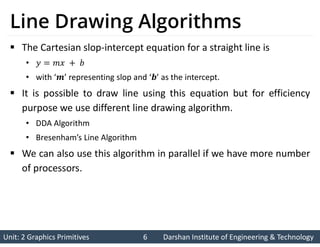
  • 6. Unit: 2 Graphics Primitives 6 Unit: 2 Graphics Primitives 6 Darshan Institute of Engineering & Technology Darshan Institute of Engineering & Technology Line Drawing Algorithms  The Cartesian slop-intercept equation for a straight line is • • with ‘ ’ representing slop and ‘ ’ as the intercept.  It is possible to draw line using this equation but for efficiency purpose we use different line drawing algorithm. • DDA Algorithm • Bresenham’s Line Algorithm  We can also use this algorithm in parallel if we have more number of processors.
  • 7. Unit: 2 Graphics Primitives 7 Unit: 2 Graphics Primitives 7 Darshan Institute of Engineering & Technology Darshan Institute of Engineering & Technology Introduction to DDA Algorithm  Full form of DDA is Digital Differential Analyzer  DDA is scan conversion line drawing algorithm based on calculating either or using line equation.  We sample the line at unit intervals in one coordinate and find corresponding integer values nearest the line path for the other coordinate.  Selecting unit interval in either or direction based on way we process line.
  • 8. Unit: 2 Graphics Primitives 8 Unit: 2 Graphics Primitives 8 Darshan Institute of Engineering & Technology Darshan Institute of Engineering & Technology Unit Step Direction in DDA Algorithm  Processing from left to right.  Slope is “+ve”, & Magnitude is Less than 1  Slope is “-ve”, & Magnitude is Less than 1  Slope is “+ve”, & Magnitude is greater than 1  Slope is “-ve”, & Magnitude is greater than 1  Processing from right to left.  Slope is “+ve”, & Magnitude is Less than 1  Slope is “-ve”, & Magnitude is Less than 1  Slope is “+ve”, & Magnitude is greater than 1  Slope is “-ve”, & Magnitude is greater than 1
  • 9. Unit: 2 Graphics Primitives 9 Unit: 2 Graphics Primitives 9 Darshan Institute of Engineering & Technology Darshan Institute of Engineering & Technology Derivation of DDA Algorithm  We sample at unit interval and calculate each successive value as follow:   [For first intermediate point]  [For 𝑡ℎ intermediate point]  [For 𝑡ℎ intermediate point]  Subtract from    Using this equation computation becomes faster than normal line equation.  As is any real value calculated value must be rounded to nearest integer.
  • 10. Unit: 2 Graphics Primitives 10 Unit: 2 Graphics Primitives 10 Darshan Institute of Engineering & Technology Darshan Institute of Engineering & Technology Contd.  We sample at unit interval and calculate each successive value as follow:   [For first intermediate point]  [For 𝑡ℎ intermediate point]  [For intermediate point] Subtract from   Similarly  for ∆x = -1: we obtain  for ∆y = -1: we obtain
  • 11. Procedure for DDA line algorithm. Void lineDDA (int xa, int ya, int xb, int yb) { int dx = xb – xa, dy = yb – ya, steps, k; float xincrement, yincrement, x = xa, y = ya; if (abs(dx)>abs(dy)) { Steps = abs (dx); } else { Steps = abs (dy); } xincrement = dx/(float) steps; yincrement = dy/(float) steps; setpixel (ROUND (x), ROUND (y)); for(k=0;k<steps;k++) { x += xincrement; y += yincrement; setpixel (ROUND (x), ROUND (y)); } }
  • 12. Unit: 2 Graphics Primitives 12 Unit: 2 Graphics Primitives 12 Darshan Institute of Engineering & Technology Darshan Institute of Engineering & Technology Example DDA Algorithm  Example: Draw line with coordinates , .   is “+ve” and less than 1 so .  , [Plot the initial point as given]  , [Plot the first intermediate point by rounding it to ]  , [Plot the second intermediate point by rounding it to ]  , [Plot the third intermediate point by rounding it to ]  , [Plot End point given] 0 1 2 3 4 5 6 7 8 4 3 2 1 0
  • 13. Unit: 2 Graphics Primitives 13 Unit: 2 Graphics Primitives 13 Darshan Institute of Engineering & Technology Darshan Institute of Engineering & Technology Introduction to Bresenham’s Line Algorithm  An accurate and efficient raster line-generating algorithm, developed by Bresenham.  It scan converts line using only incremental integer calculations.  That can be modified to display circles and other curves.  Based on slop we take unit step in one direction and decide pixel of other direction from two candidate pixel.  If we sample at unit interval and vice versa.
  • 14. Unit: 2 Graphics Primitives 14 Unit: 2 Graphics Primitives 14 Darshan Institute of Engineering & Technology Darshan Institute of Engineering & Technology Line Path & Candidate pixel  Example |ΔX| > |ΔY|, and ΔY is “+ve”.  Initial point (Xk, Yk)  Line path  Candidate pixels {(Xk+1, Yk), (Xk+1, Yk+1)} 0 1 2 3 4 4 3 2 1 0  Now we need to decide which candidate pixel is more closer to actual line.  For that we use decision parameter (Pk) equation.  Decision parameter can be derived by calculating distance of actual line from two candidate pixel.
  • 15. Unit: 2 Graphics Primitives 15 Unit: 2 Graphics Primitives 15 Darshan Institute of Engineering & Technology Darshan Institute of Engineering & Technology Derivation Bresenham’s Line Algorithm  [Line Equation]  [Actual Y value at Xk position]  [Actual Y value at Xk +1position] Distance between actual line position and lower candidate pixel   Distance between actual line position and upper candidate pixel   0 1 2 3 4 4 3 2 1 0
  • 16. Unit: 2 Graphics Primitives 16 Unit: 2 Graphics Primitives 16 Darshan Institute of Engineering & Technology Darshan Institute of Engineering & Technology Contd. Calculate     [Put ] Decision parameter     [Replacing single constant C for simplicity] Similarly 
  • 17. Unit: 2 Graphics Primitives 17 Unit: 2 Graphics Primitives 17 Darshan Institute of Engineering & Technology Darshan Institute of Engineering & Technology Contd. Subtract from   [where ]  [where depending on selection of previous pixel]
  • 18. Unit: 2 Graphics Primitives 18 Unit: 2 Graphics Primitives 18 Darshan Institute of Engineering & Technology Darshan Institute of Engineering & Technology Initial Decision parameter  The first decision parameter is calculated using equation of .   [Put ]  [Substitute 0 0]  [Substitute ]   [Initial decision parameter with all terms are constant]
  • 19. Unit: 2 Graphics Primitives 19 Unit: 2 Graphics Primitives 19 Darshan Institute of Engineering & Technology Darshan Institute of Engineering & Technology Bresenham’s Line Algorithm 1. Input the two line endpoints and store the left endpoint in . 2. Load into the frame buffer; that is, plot the first point. 3. Calculate constants , , , and , and obtain the starting value for the decision parameter as 4. At each along the line, starting at , perform the following test: If , the next point to plot is and Otherwise, the next point to plot is and 5. Repeat step-4 times.
  • 20. Unit: 2 Graphics Primitives 20 Unit: 2 Graphics Primitives 20 Darshan Institute of Engineering & Technology Darshan Institute of Engineering & Technology Discryption of Bresenham’s Line Algorithm  Bresenham’s algorithm is generalized to lines with arbitrary slope.  For lines with positive slope greater than 1 we interchange the roles of the and directions.  Also we can revise algorithm to draw line from right endpoint to left endpoint, both and decrease as we step from right to left.  When 𝑘 we can choose either lower or upper pixel but same for whole line.  For the negative slope the procedure are similar except that now one coordinate decreases as the other increases.  The special case handle separately by loading directly into the frame buffer without processing.  Horizontal line ,  Vertical line  Diagonal line with
  • 21. Unit: 2 Graphics Primitives 21 Unit: 2 Graphics Primitives 21 Darshan Institute of Engineering & Technology Darshan Institute of Engineering & Technology Example Bresenham’s Line Algorithm  Example: Draw line with coordinates , .  Plot left end point .  Calculate: • , • , • , • ,   Now so we select upper pixel .   Now so we select lower pixel .   Now so we select upper pixel .   Now so we select lower pixel . 0 1 2 3 4 5 6 7 8 4 3 2 1 0
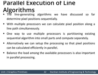
  • 22. Unit: 2 Graphics Primitives 22 Unit: 2 Graphics Primitives 22 Darshan Institute of Engineering & Technology Darshan Institute of Engineering & Technology Parallel Execution of Line Algorithms  The line-generating algorithms we have discussed so far determine pixel positions sequentially.  With multiple processors we can calculate pixel position along a line path simultaneously.  One way to use multiple processors is partitioning existing sequential algorithm into small parts and compute separately.  Alternatively we can setup the processing so that pixel positions can be calculated efficiently in parallel.  Balance the load among the available processors is also important in parallel processing.
  • 23. Unit: 2 Graphics Primitives 23 Unit: 2 Graphics Primitives 23 Darshan Institute of Engineering & Technology Darshan Institute of Engineering & Technology Parallel Bresenham Line Algorithms  For number of processors we can set up parallel Bresenham line algorithm by subdividing the line path into partitions and simultaneously generating line segment in each of the subintervals.  For a line with slope and left endpoint coordinate position , we partition the line along the positive direction.  The distance between beginning positions of adjacent partitions can be calculated as:  Where is the width of the line and value for partition with is computed using integer division.
  • 24. Unit: 2 Graphics Primitives 24 Unit: 2 Graphics Primitives 24 Darshan Institute of Engineering & Technology Darshan Institute of Engineering & Technology Contd.  Numbering the partitions and the processors, as 0, 1, 2, up to , we calculate the starting coordinate for the partition as:  The change in the direction over each partition is calculated from the line slope and partition width :  At the partition, the starting y coordinate is then
  • 25. Unit: 2 Graphics Primitives 25 Unit: 2 Graphics Primitives 25 Darshan Institute of Engineering & Technology Darshan Institute of Engineering & Technology IDP for Parallel Bresenham Line Algorithms  The initial decision parameter(IDP) for Bresenham's algorithm at the start of the subinterval is obtained as follow:   ∆ ∆    Each processor then calculates pixel positions over its assigned subinterval.
  • 26. Unit: 2 Graphics Primitives 26 Unit: 2 Graphics Primitives 26 Darshan Institute of Engineering & Technology Darshan Institute of Engineering & Technology Other Ways for Parallel Execution of Line Algorithms  For line with slope greater than 1 we partitioning the line in the direction and calculating beginning values for the positions.  For negative slopes, we increment coordinate values in one direction and decrement in the other.  Another way to set up parallel algorithms on raster system is to assign each processor to a particular group of screen pixels.  With sufficient number of processor we can assign each processor to one pixel within some screen region.  This can be done by assigning one processor to each of the pixels within the limit of the bounding rectangle.
  • 27. Unit: 2 Graphics Primitives 27 Unit: 2 Graphics Primitives 27 Darshan Institute of Engineering & Technology Darshan Institute of Engineering & Technology Contd.  Perpendicular distance d from line to a particular pixel is calculated by:  Where    With   , , and are constant we need to compute only once.
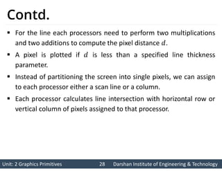
  • 28. Unit: 2 Graphics Primitives 28 Unit: 2 Graphics Primitives 28 Darshan Institute of Engineering & Technology Darshan Institute of Engineering & Technology Contd.  For the line each processors need to perform two multiplications and two additions to compute the pixel distance .  A pixel is plotted if is less than a specified line thickness parameter.  Instead of partitioning the screen into single pixels, we can assign to each processor either a scan line or a column.  Each processor calculates line intersection with horizontal row or vertical column of pixels assigned to that processor.
  • 29. Unit: 2 Graphics Primitives 29 Unit: 2 Graphics Primitives 29 Darshan Institute of Engineering & Technology Darshan Institute of Engineering & Technology Contd.  If vertical column is assign to processor then is fix and it will calculate .  Similarly if horizontal row is assign to processor then is fix and will be calculated.  Such direct methods are slow in sequential machine but we can perform very efficiently using multiple processors.
  • 30. Unit: 2 Graphics Primitives 30 Unit: 2 Graphics Primitives 30 Darshan Institute of Engineering & Technology Darshan Institute of Engineering & Technology Circle  A circle is defined as the set of points that are all at a given distance from a center position say . Center r Radius
  • 31. Unit: 2 Graphics Primitives 31 Unit: 2 Graphics Primitives 31 Darshan Institute of Engineering & Technology Darshan Institute of Engineering & Technology Properties of Circle- Cartesion Coordinate  Cartesian coordinates equation :   We could use this equation to calculate circular boundary points.  We increment 1 in direction in every steps from to and calculate corresponding values at each position as:    
  • 32. Unit: 2 Graphics Primitives 32 Unit: 2 Graphics Primitives 32 Darshan Institute of Engineering & Technology Darshan Institute of Engineering & Technology Contd.  But this is not best method as it requires more number of calculations which take more time to execute.  And also spacing between the plotted pixel positions is not uniform.  We can adjust spacing by stepping through y values and calculating x values whenever the absolute value of the slop of the circle is greater than 1.  But it will increases computation time.
  • 33. Unit: 2 Graphics Primitives 33 Unit: 2 Graphics Primitives 33 Darshan Institute of Engineering & Technology Darshan Institute of Engineering & Technology Properties of Circle- Polar Coordinate  Another way to eliminate the non-uniform spacing is to draw circle using polar coordinates ‘r’ and ‘’.  Calculating circle boundary using polar equation is given by pair of equations which is as follows.    When display is produce using these equations using fixed angular step size circle is plotted with uniform spacing.  The step size ‘’ is chosen according to application and display device.  For a more continuous boundary on a raster display we can set the step size at .
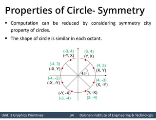
  • 34. Unit: 2 Graphics Primitives 34 Unit: 2 Graphics Primitives 34 Darshan Institute of Engineering & Technology Darshan Institute of Engineering & Technology Properties of Circle- Symmetry  Computation can be reduced by considering symmetry city property of circles.  The shape of circle is similar in each octant. 𝑂 (X, Y) (Y, X) (X, -Y) (Y, -X) (-X, -Y) (-Y, -X) (-Y, X) (-X, Y) (4, 3) (3, 4) (4, -3) (3, -4) (-4, -3) (-3, -4) (-3, 4) (-4, 3)
  • 35. Unit: 2 Graphics Primitives 35 Unit: 2 Graphics Primitives 35 Darshan Institute of Engineering & Technology Darshan Institute of Engineering & Technology Circle Algorithm  Taking advantage of this symmetry property of circle we can generate all pixel position on boundary of circle by calculating only one sector from to .  Determining pixel position along circumference of circle using any of two equations shown above still required large computation.  More efficient circle algorithm are based on incremental calculation of decision parameters, as in the Bresenham line algorithm.  Bresenham’s line algorithm can be adapted to circle generation by setting decision parameter for finding closest pixel to the circumference at each sampling step.
  • 36. Unit: 2 Graphics Primitives 36 Unit: 2 Graphics Primitives 36 Darshan Institute of Engineering & Technology Darshan Institute of Engineering & Technology Contd.  A method for direct distance comparison to test the midpoint between two pixels to determine if this midpoint is inside or outside the circle boundary.  This method is easily applied to other conics also.  Midpoint approach generates same pixel position as generated by bresenham’s circle algorithm.  The error involve in locating pixel positions along any conic section using midpoint test is limited to one-half the pixel separation.
  • 37. Unit: 2 Graphics Primitives 37 Unit: 2 Graphics Primitives 37 Darshan Institute of Engineering & Technology Darshan Institute of Engineering & Technology Introduction to Midpoint Circle Algorithm  In this we sample at unit interval and determine the closest pixel position to the specified circle path at each step.  Given radius and center  We first setup our algorithm to calculate circular path coordinates for center .  And then we will transfer calculated pixel position to center by adding to and to .  Along the circle section from to in the first quadrant, the slope of the curve varies from to .  So we can step unit step in positive direction over this octant and use a decision parameter to determine which of the two possible position is closer to the circular path.
  • 38. Unit: 2 Graphics Primitives 38 Unit: 2 Graphics Primitives 38 Darshan Institute of Engineering & Technology Darshan Institute of Engineering & Technology Decision Parameter Midpoint Circle Algorithm  Position in the other seven octants are then obtain by symmetry.  For the decision parameter we use the circle function which is:  Above equation we calculate for the mid positions between pixels near the circular path at each sampling step.  And we setup incremental calculation for this function as we did in the line algorithm.
  • 39. Unit: 2 Graphics Primitives 39 Unit: 2 Graphics Primitives 39 Darshan Institute of Engineering & Technology Darshan Institute of Engineering & Technology Midpoint between Candidate pixel  Figure shows the midpoint between the two candidate pixels at sampling position .  Assuming we have just plotted the pixel at  Next we determine whether the pixel at position or the one at position is closer to circle boundary. Midpoint Candidate Pixel
  • 40. Unit: 2 Graphics Primitives 40 Unit: 2 Graphics Primitives 40 Darshan Institute of Engineering & Technology Darshan Institute of Engineering & Technology Derivation Midpoint Circle Algorithm  So for finding which pixel is more closer using decision parameter evaluated at the midpoint between two candidate pixels as below:    If , midpoint is inside the circle and the pixel on the scan line is closer to circle boundary.  Otherwise midpoint is outside or on the boundary and we select the scan line .
  • 41. Unit: 2 Graphics Primitives 41 Unit: 2 Graphics Primitives 41 Darshan Institute of Engineering & Technology Darshan Institute of Engineering & Technology Contd.  Successive decision parameters are obtain using incremental calculations as follows:    Now we can obtain recursive calculation using equation of and as follow  
  • 42. Unit: 2 Graphics Primitives 42 Unit: 2 Graphics Primitives 42 Darshan Institute of Engineering & Technology Darshan Institute of Engineering & Technology Contd.      Now we can put 
  • 43. Unit: 2 Graphics Primitives 43 Unit: 2 Graphics Primitives 43 Darshan Institute of Engineering & Technology Darshan Institute of Engineering & Technology Contd.   In above equation is either or depending on the sign of the .  If we select .   If we select .    
  • 44. Unit: 2 Graphics Primitives 44 Unit: 2 Graphics Primitives 44 Darshan Institute of Engineering & Technology Darshan Institute of Engineering & Technology Contd.    Now put . 
  • 45. Unit: 2 Graphics Primitives 45 Unit: 2 Graphics Primitives 45 Darshan Institute of Engineering & Technology Darshan Institute of Engineering & Technology IDP Midpoint Circle Algorithm  The initial decision parameter(IDP) is obtained by evaluating the circle function at the start position as follows.     
  • 46. Algorithm for Midpoint Circle Generation 1. Input radius r and circle center , and obtain the first point on the circumference of a circle centered on the origin as 2. calculate the initial value of the decision parameter as 3. At each position, starting at , perform the following test: If , the next point along the circle centered on is Otherwise, the next point along the circle is Where , & . 4. Determine symmetry points in the other seven octants. 5. Move each calculated pixel position onto the circular path centered on and plot the coordinate values: , 6. Repeat steps 3 through 5 until .
  • 47. Unit: 2 Graphics Primitives 47 Unit: 2 Graphics Primitives 47 Darshan Institute of Engineering & Technology Darshan Institute of Engineering & Technology  Example: Draw circle with radius , and center of circle is (Only one octant to )  First we find pixel position for octant to for center    Now we select (1, 10)    Now we select (2, 10) Example Midpoint Circle Algorithm 𝒌 𝟏 𝒌 𝟏 𝒌 (1, 10) -9 0 (2, 10) -6 1 (3, 10) -1 2 (4, 9) 6 3 (5, 9) -3 4 (6, 8) 8 5 (7, 7) 5 6
  • 48. Unit: 2 Graphics Primitives 48 Unit: 2 Graphics Primitives 48 Darshan Institute of Engineering & Technology Darshan Institute of Engineering & Technology    Now we select (3, 10)    Now we select (4, 9)    Now we select (5, 9) Contd. 𝒌 𝟏 𝒌 𝟏 𝒌 (1, 10) -9 0 (2, 10) -6 1 (3, 10) -1 2 (4, 9) 6 3 (5, 9) -3 4 (6, 8) 8 5 (7, 7) 5 6
  • 49. Unit: 2 Graphics Primitives 49 Unit: 2 Graphics Primitives 49 Darshan Institute of Engineering & Technology Darshan Institute of Engineering & Technology    Now we select (6, 8)    Now we select (7, 7)  Now Loop exit as , as  in our case Contd. 𝒌 𝟏 𝒌 𝟏 𝒌 (1, 10) -9 0 (2, 10) -6 1 (3, 10) -1 2 (4, 9) 6 3 (5, 9) -3 4 (6, 8) 8 5 (7, 7) 5 6
  • 50. Unit: 2 Graphics Primitives 50 Unit: 2 Graphics Primitives 50 Darshan Institute of Engineering & Technology Darshan Institute of Engineering & Technology Contd.  Than we calculate pixel position for given center using equations:   Center (1, 1) Center (0, 0) (2, 11) (1, 10) (3, 11) (2, 10) (4, 11) (3, 10) (5, 10) (4, 9) (6, 10) (5, 9) (7, 9) (6, 8) (8, 8) (7, 7)
  • 51. Unit: 2 Graphics Primitives 51 Unit: 2 Graphics Primitives 51 Darshan Institute of Engineering & Technology Darshan Institute of Engineering & Technology Contd.  Plot the pixel.  First plot initial point. (1, 11) Center (1, 1) (2, 11) (3, 11) (4, 11) (5, 10) (6, 10) (7, 9) (8, 8) 12 11 10 9 8 7 6 5 4 3 2 1 0 0 1 2 3 4 5 6 7 8 9 10 11 Center (1, 1)
  • 52. Unit: 2 Graphics Primitives 52 Unit: 2 Graphics Primitives 52 Darshan Institute of Engineering & Technology Darshan Institute of Engineering & Technology Ellipse  AN ellipse is defined as the set of points such that the sum of the distances from two fixed positions (foci) is same for all points.
  • 53. Unit: 2 Graphics Primitives 53 Unit: 2 Graphics Primitives 53 Darshan Institute of Engineering & Technology Darshan Institute of Engineering & Technology Contd.  If we labeled distance from two foci to any point on ellipse boundary as and then the general equation of an ellipse can be written as:  Expressing distance in terms of focal coordinates and we have  [Using Distance formula]
  • 54. Unit: 2 Graphics Primitives 54 Unit: 2 Graphics Primitives 54 Darshan Institute of Engineering & Technology Darshan Institute of Engineering & Technology Properties of Ellipse-Specifying Equations  An interactive method for specifying an ellipse in an arbitrary orientation is to input  two foci and  a point on the ellipse boundary.  With this three coordinates we can evaluate constant in equation:  We can also write this equation in the form  Where the coefficients , and are evaluated in terms of the focal coordinates and the dimensions of the major and minor axes of the ellipse.
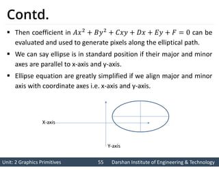
  • 55. Unit: 2 Graphics Primitives 55 Unit: 2 Graphics Primitives 55 Darshan Institute of Engineering & Technology Darshan Institute of Engineering & Technology Contd.  Then coefficient in can be evaluated and used to generate pixels along the elliptical path.  We can say ellipse is in standard position if their major and minor axes are parallel to x-axis and y-axis.  Ellipse equation are greatly simplified if we align major and minor axis with coordinate axes i.e. x-axis and y-axis. X-axis Y-axis
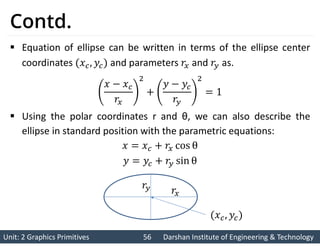
  • 56. Unit: 2 Graphics Primitives 56 Unit: 2 Graphics Primitives 56 Darshan Institute of Engineering & Technology Darshan Institute of Engineering & Technology Contd.  Equation of ellipse can be written in terms of the ellipse center coordinates and parameters and as.  Using the polar coordinates r and θ, we can also describe the ellipse in standard position with the parametric equations:
  • 57. Unit: 2 Graphics Primitives 57 Unit: 2 Graphics Primitives 57 Darshan Institute of Engineering & Technology Darshan Institute of Engineering & Technology  Symmetry property further reduced computations.  An ellipse in standard position is symmetric between quadrant. Properties of Ellipse-Symmetry
  • 58. Unit: 2 Graphics Primitives 58 Unit: 2 Graphics Primitives 58 Darshan Institute of Engineering & Technology Darshan Institute of Engineering & Technology Introduction to Midpoint Ellipse Algorithm  Given parameters .  We determine points for an ellipse in standard position centered on the origin.  Then we shift the points so the ellipse is centered at .  If we want to display the ellipse in nonstandard position then we rotate the ellipse about its center to align with required direction.  For the present we consider only the standard position.  We draw ellipse in first quadrant and than use symmetry property for other three quadrant.
  • 59. Unit: 2 Graphics Primitives 59 Unit: 2 Graphics Primitives 59 Darshan Institute of Engineering & Technology Darshan Institute of Engineering & Technology  In this method we divide first quadrant into two parts according to the slope of an ellipse  Boundary divides region at • slope = -1.  We take unit step in X direction • If magnitude of ellipse slope < 1 (Region 1).  We take unit step in Y direction • If magnitude of ellipse slope > 1 (Region 2). Regions in Midpoint Ellipse Algorithm Region 1 Region 2
  • 60. Unit: 2 Graphics Primitives 60 Unit: 2 Graphics Primitives 60 Darshan Institute of Engineering & Technology Darshan Institute of Engineering & Technology Ways of Processing Midpoint Ellipse Algorithm  We can start from and step clockwise along the elliptical path in the first quadrant  Alternatively, we could start at and select points in a counterclockwise order.  With parallel processors, we could calculate pixel positions in the two regions simultaneously.  Here we consider sequential implementation of midpoint algorithm.  We take the start position at and steps along the elliptical path in clockwise order through the first quadrant.
  • 61. Unit: 2 Graphics Primitives 61 Unit: 2 Graphics Primitives 61 Darshan Institute of Engineering & Technology Darshan Institute of Engineering & Technology Decision Parameter Midpoint Ellipse Algorithm  We define ellipse function for center of ellipse at (0, 0) as follows.   Which has the following properties:  Thus the ellipse function serves as the decision parameter in the midpoint ellipse algorithm.  At each sampling position we select the next pixel from two candidate pixel.
  • 62. Unit: 2 Graphics Primitives 62 Unit: 2 Graphics Primitives 62 Darshan Institute of Engineering & Technology Darshan Institute of Engineering & Technology Processing Steps of Midpoint Ellipse Algorithm  Starting at we take unit step in direction until we reach the boundary between region-1 and region-2.  Then we switch to unit steps in direction in remaining portion on ellipse in first quadrant. Region 1 Region 2  At each step we need to test the value of the slope of the curve for deciding the end point of the region-1.
  • 63. Unit: 2 Graphics Primitives 63 Unit: 2 Graphics Primitives 63 Darshan Institute of Engineering & Technology Darshan Institute of Engineering & Technology Decide Boundary between Region 1 and 2  The ellipse slope is calculated using following equation.   At boundary between region 1 and 2 slope= -1 and equation become.   Therefore we move out of region 1 whenever following equation is false: 
  • 64. Unit: 2 Graphics Primitives 64 Unit: 2 Graphics Primitives 64 Darshan Institute of Engineering & Technology Darshan Institute of Engineering & Technology Midpoint between Candidate pixel in Region 1  Figure shows the midpoint between the two candidate pixels at sampling position in the first region.  Assume we are at position and we determine the next position along the ellipse path, by evaluating decision parameter at midpoint between two candidate pixels.  k k k k k y 2 2 x 2 2 x 2 y 2 Midpoint Candidate Pixel
  • 65. Unit: 2 Graphics Primitives 65 Unit: 2 Graphics Primitives 65 Darshan Institute of Engineering & Technology Darshan Institute of Engineering & Technology Derivation for Region 1    If , the midpoint is inside the ellipse and the pixel on scan line is closer to ellipse boundary  Otherwise the midpoint is outside or on the ellipse boundary and we select the pixel .
  • 66. Unit: 2 Graphics Primitives 66 Unit: 2 Graphics Primitives 66 Darshan Institute of Engineering & Technology Darshan Institute of Engineering & Technology Contd.  At the next sampling position decision parameter for region 1 is evaluated as.    Now subtract from 
  • 67. Unit: 2 Graphics Primitives 67 Unit: 2 Graphics Primitives 67 Darshan Institute of Engineering & Technology Darshan Institute of Engineering & Technology Contd.     Now making as subject. 
  • 68. Unit: 2 Graphics Primitives 68 Unit: 2 Graphics Primitives 68 Darshan Institute of Engineering & Technology Darshan Institute of Engineering & Technology Contd.   is either or , depends on the sign of
  • 69. Unit: 2 Graphics Primitives 69 Unit: 2 Graphics Primitives 69 Darshan Institute of Engineering & Technology Darshan Institute of Engineering & Technology IDP for Region 1  Now we calculate the initial decision parameter by putting as follow.    
  • 70. Unit: 2 Graphics Primitives 70 Unit: 2 Graphics Primitives 70 Darshan Institute of Engineering & Technology Darshan Institute of Engineering & Technology Midpoint between Candidate pixel in Region 2  Now we similarly calculate over region-2.  Unit stepping in negative direction and the midpoint is now taken between horizontal pixels at each step.  For this region, the decision parameter is evaluated as follows.  k+2 k+1 k k k-1 y 2 2 x 2 2 x 2 y 2 Midpoint Candidate Pixel
  • 71. Unit: 2 Graphics Primitives 71 Unit: 2 Graphics Primitives 71 Darshan Institute of Engineering & Technology Darshan Institute of Engineering & Technology Derivation for Region 2    If the midpoint is outside the ellipse boundary, and we select the pixel at .  If the midpoint is inside or on the ellipse boundary and we select .
  • 72. Unit: 2 Graphics Primitives 72 Unit: 2 Graphics Primitives 72 Darshan Institute of Engineering & Technology Darshan Institute of Engineering & Technology Contd.  At the next sampling position decision parameter for region 2 is evaluated as.    Now subtract from 
  • 73. Unit: 2 Graphics Primitives 73 Unit: 2 Graphics Primitives 73 Darshan Institute of Engineering & Technology Darshan Institute of Engineering & Technology Contd.    
  • 74. Unit: 2 Graphics Primitives 74 Unit: 2 Graphics Primitives 74 Darshan Institute of Engineering & Technology Darshan Institute of Engineering & Technology Contd.   Now making as subject.   Here is either or , depends on the sign of .
  • 75. Unit: 2 Graphics Primitives 75 Unit: 2 Graphics Primitives 75 Darshan Institute of Engineering & Technology Darshan Institute of Engineering & Technology IDP for Region 2  In region-2 initial position is selected which is last position of region one and the initial decision parameter is calculated as follows.    For simplify calculation of we could also select pixel position in counterclockwise order starting at .
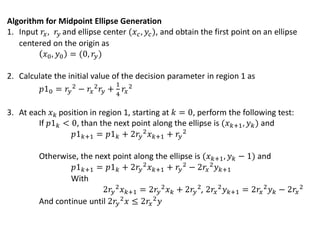
  • 76. Algorithm for Midpoint Ellipse Generation 1. Input and ellipse center , and obtain the first point on an ellipse centered on the origin as 2. Calculate the initial value of the decision parameter in region 1 as 3. At each position in region 1, starting at , perform the following test: If , than the next point along the ellipse is and Otherwise, the next point along the ellipse is and With , And continue until
  • 77. Contd. 4. Calculate the initial value of the decision parameter in region 2 using the last point calculated in region 1 as 5. At each position in region-2, starting at , perform the following test: If , the next point along the ellipse is and Otherwise, the next point along the ellipse is and Using the same incremental calculations for and as in region 1. 6. Determine symmetry points in the other three quadrants. 7. Move each calculated pixel position onto the elliptical path centered on and plot the coordinate values: , 8. Repeat the steps for region 2 until .
  • 78. Unit: 2 Graphics Primitives 78 Unit: 2 Graphics Primitives 78 Darshan Institute of Engineering & Technology Darshan Institute of Engineering & Technology Example Midpoint Ellipse Algorithm  Example: Calculate intermediate pixel position (For first quadrant) for ellipse with and ellipse center is at origin  Initial point   
  • 79. Unit: 2 Graphics Primitives 79 Unit: 2 Graphics Primitives 79 Darshan Institute of Engineering & Technology Darshan Institute of Engineering & Technology Contd. (xk+1, yk+1) p1k K (1, 6) -332 0 (2, 6) -224 1 (3, 6) -44 2 (4, 5) 208 3 (5, 5) -108 4 (6, 4) 288 5 (7, 3) 244 6   
  • 80. Unit: 2 Graphics Primitives 80 Unit: 2 Graphics Primitives 80 Darshan Institute of Engineering & Technology Darshan Institute of Engineering & Technology Contd. (xk+1, yk+1) p1k K (1, 6) -332 0 (2, 6) -224 1 (3, 6) -44 2 (4, 5) 208 3 (5, 5) -108 4 (6, 4) 288 5 (7, 3) 244 6  
  • 81. Unit: 2 Graphics Primitives 81 Unit: 2 Graphics Primitives 81 Darshan Institute of Engineering & Technology Darshan Institute of Engineering & Technology Contd. (xk+1, yk+1) p1k K (1, 6) -332 0 (2, 6) -224 1 (3, 6) -44 2 (4, 5) 208 3 (5, 5) -108 4 (6, 4) 288 5 (7, 3) 244 6  
  • 82. Unit: 2 Graphics Primitives 82 Unit: 2 Graphics Primitives 82 Darshan Institute of Engineering & Technology Darshan Institute of Engineering & Technology Contd. (xk+1, yk+1) p1k K (1, 6) -332 0 (2, 6) -224 1 (3, 6) -44 2 (4, 5) 208 3 (5, 5) -108 4 (6, 4) 288 5 (7, 3) 244 6  
  • 83. Unit: 2 Graphics Primitives 83 Unit: 2 Graphics Primitives 83 Darshan Institute of Engineering & Technology Darshan Institute of Engineering & Technology Contd. (xk+1, yk+1) p1k K (1, 6) -332 0 (2, 6) -224 1 (3, 6) -44 2 (4, 5) 208 3 (5, 5) -108 4 (6, 4) 288 5 (7, 3) 244 6  
  • 84. Unit: 2 Graphics Primitives 84 Unit: 2 Graphics Primitives 84 Darshan Institute of Engineering & Technology Darshan Institute of Engineering & Technology Contd. (xk+1, yk+1) p1k K (1, 6) -332 0 (2, 6) -224 1 (3, 6) -44 2 (4, 5) 208 3 (5, 5) -108 4 (6, 4) 288 5 (7, 3) 244 6  
  • 85. Unit: 2 Graphics Primitives 85 Unit: 2 Graphics Primitives 85 Darshan Institute of Engineering & Technology Darshan Institute of Engineering & Technology Contd. (xk+1, yk+1) p2k K (8, 2) -23 0 (8, 1) 361 1 (8, 0) 297 2  
  • 86. Unit: 2 Graphics Primitives 86 Unit: 2 Graphics Primitives 86 Darshan Institute of Engineering & Technology Darshan Institute of Engineering & Technology Contd. (xk+1, yk+1) p2k K (8, 2) -23 0 (8, 1) 361 1 (8, 0) 297 2  
  • 87. Unit: 2 Graphics Primitives 87 Unit: 2 Graphics Primitives 87 Darshan Institute of Engineering & Technology Darshan Institute of Engineering & Technology Contd. (xk+1, yk+1) p2k K (8, 2) -23 0 (8, 1) 361 1 (8, 0) 297 2  
  • 88. Unit: 2 Graphics Primitives 88 Unit: 2 Graphics Primitives 88 Darshan Institute of Engineering & Technology Darshan Institute of Engineering & Technology Contd.  Plot the pixel.  Plot initial point(0, 6) Center (0, 0) (1, 6) (2, 6) (3, 6) (4, 5) (5, 5) (6, 4) (7, 3) 12 11 10 9 8 7 6 5 4 3 2 1 0 0 1 2 3 4 5 6 7 8 9 10 11 Center (0, 0) Center (0, 0) (8, 2) (8, 1) (8, 0)
  • 89. Unit: 2 Graphics Primitives 89 Unit: 2 Graphics Primitives 89 Darshan Institute of Engineering & Technology Darshan Institute of Engineering & Technology Filled-Area Primitives  In practical we often use polygon which are filled with some colour or pattern inside it.  There are two basic approaches to area filling on raster systems. • One way to fill an area is to determine the overlap intervals for scan line that cross the area. • Another method is to start from a given interior position and paint outward from this point until we encounter boundary.
  • 90. Unit: 2 Graphics Primitives 90 Unit: 2 Graphics Primitives 90 Darshan Institute of Engineering & Technology Darshan Institute of Engineering & Technology Scan-Line Polygon Fill Algorithm  For each scan-line crossing a polygon, the algorithm locates the intersection points are of scan line with the polygon edges.  This intersection points are stored from left to right.  Frame buffer positions between each pair of intersection point are set to specified fill color. Scan line
  • 91. Unit: 2 Graphics Primitives 91 Unit: 2 Graphics Primitives 91 Darshan Institute of Engineering & Technology Darshan Institute of Engineering & Technology Contd.  Scan line intersects at vertex are required special handling.  For vertex we must look at the other endpoints of the two line segments which meet at this vertex. • If these points lie on the same (up or down) side of the scan line, then that point is counts as two intersection points. • If they lie on opposite sides of the scan line, then the point is counted as single intersection. Scan line Scan line Scan line
  • 92. Unit: 2 Graphics Primitives 92 Unit: 2 Graphics Primitives 92 Darshan Institute of Engineering & Technology Darshan Institute of Engineering & Technology Edge Intersection Calculation with Scan-Line  Coherence methods often involve incremental calculations applied along a single scan line or between successive scan lines.  In determining edge intersections, we can set up incremental coordinate calculations along any edge by exploiting the fact that the slope of the edge is constant from one scan line to the next.  For above figure we can write slope equation for polygon boundary as follows.   Since change in coordinates between the two scan lines is simply 
  • 93. Unit: 2 Graphics Primitives 93 Unit: 2 Graphics Primitives 93 Darshan Institute of Engineering & Technology Darshan Institute of Engineering & Technology Contd.  So slope equation can be modified as follows      Each successive intercept can thus be calculated by adding the inverse of the slope and rounding to the nearest integer.
  • 94. Unit: 2 Graphics Primitives 94 Unit: 2 Graphics Primitives 94 Darshan Institute of Engineering & Technology Darshan Institute of Engineering & Technology Edge Intersection Calculation with Scan-Line for parallel execution  For parallel execution of this algorithm we assign each scan line to separate processor in that case instead of using previous values for calculation we use initial values by using equation as.   Now if we put in incremental calculation equation then we obtain equation as.   Using this equation we can perform integer evaluation of intercept.
  • 95. Unit: 2 Graphics Primitives 95 Unit: 2 Graphics Primitives 95 Darshan Institute of Engineering & Technology Darshan Institute of Engineering & Technology Simplified Method for Edge Intersection Calculation with Scan-Line 1. Suppose 2. Initially, set counter to , and increment to (which is ). 3. When move to next scan line, increment counter by adding 4. When counter is equal to or greater than (which is ), increment the (in other words, the for this scan line is one more than the previous scan line), and decrement counter by (which is ). Counter=0 Counter=3 Counter=6 Counter=2 Counter=5 Counter=1 Counter=4 Counter=0
  • 96. Unit: 2 Graphics Primitives 96 Unit: 2 Graphics Primitives 96 Darshan Institute of Engineering & Technology Darshan Institute of Engineering & Technology Use of Sorted Edge table in Scan-Line Polygon Fill Algorithm  To efficiently perform a polygon fill, we can first store the polygon boundary in a sorted edge table.  It contains all the information necessary to process the scan lines efficiently.  We use bucket sort to store the edge sorted on the smallest value of each edge in the correct scan line positions.  Only the non-horizontal edges are entered into the sorted edge table.
  • 97. Unit: 2 Graphics Primitives 97 Unit: 2 Graphics Primitives 97 Darshan Institute of Engineering & Technology Darshan Institute of Engineering & Technology Contd. A B C D C E Scan Line Scan Line Scan Line 0 1 . . . . . . . . . Scan Line Number
  • 98. Unit: 2 Graphics Primitives 98 Unit: 2 Graphics Primitives 98 Darshan Institute of Engineering & Technology Darshan Institute of Engineering & Technology Inside-Outside Tests  In area filling and other graphics operation often required to find particular point is inside or outside the polygon.  For finding which region is inside or which region is outside most graphics package use either 1. Odd even rule OR 2. Nonzero winding number rule
  • 99. Unit: 2 Graphics Primitives 99 Unit: 2 Graphics Primitives 99 Darshan Institute of Engineering & Technology Darshan Institute of Engineering & Technology Odd Even/ Odd Parity/ Even Odd Rule  By conceptually drawing a line from any position to a distant point outside the coordinate extents of the object.  Than counting the number of edges crossing by this line. 1. If Edge count is odd, than p is an interior point. 2. Otherwise p is exterior point.  To obtain accurate edge count we must sure that line selected is does not pass from any vertices. Boundary of Screen 1 1 2
  • 100. Unit: 2 Graphics Primitives 100 Unit: 2 Graphics Primitives 100 Darshan Institute of Engineering & Technology Darshan Institute of Engineering & Technology Nonzero Winding Number Rule  This method counts the number of times the polygon edges wind around a particular point in the counterclockwise direction.  This count is called the winding number.  We apply this rule by initializing winding number with 0.  Then draw a line for any point to distant point beyond the coordinate extents of the object. Boundary of Screen Winding number=0
  • 101. Unit: 2 Graphics Primitives 101 Unit: 2 Graphics Primitives 101 Darshan Institute of Engineering & Technology Darshan Institute of Engineering & Technology Contd.  The line we choose must not pass through vertices.  Then we move along that line we find number of intersecting edges. 1. If edge cross our line from right to left We add 1 to winding number 2. Otherwise subtract 1 from winding number  IF the final value of winding number is nonzero then the point is interior otherwise point is exterior. Boundary of Screen -1 +1 -1 Winding number=0 Winding number=-1 Winding number=+1-1=0
  • 102. Unit: 2 Graphics Primitives 102 Unit: 2 Graphics Primitives 102 Darshan Institute of Engineering & Technology Darshan Institute of Engineering & Technology Comparison between Odd Even Rule and Nonzero Winding Rule  For standard polygons and simple object both rule gives same result but for more complicated shape both rule gives different result. Odd Even Rule Nonzero Winding Rule
  • 103. Unit: 2 Graphics Primitives 103 Unit: 2 Graphics Primitives 103 Darshan Institute of Engineering & Technology Darshan Institute of Engineering & Technology Scan-Line Fill of Curved Boundary Areas  Scan-line fill of region with curved boundary is more time consuming as intersection calculation now involves nonlinear boundaries.  For simple curve such as circle or ellipse scan line fill process is straight forward process.  We calculate the two scan line intersection on opposite side of the curve.  This is same as generating pixel position along the curve boundary using standard equation of curve.  Then we fill the color between two boundary intersections.  Symmetry property is used to reduce the calculation.
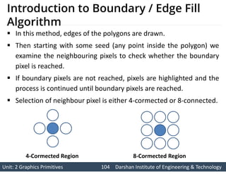
  • 104. Unit: 2 Graphics Primitives 104 Unit: 2 Graphics Primitives 104 Darshan Institute of Engineering & Technology Darshan Institute of Engineering & Technology Introduction to Boundary / Edge Fill Algorithm  In this method, edges of the polygons are drawn.  Then starting with some seed (any point inside the polygon) we examine the neighbouring pixels to check whether the boundary pixel is reached.  If boundary pixels are not reached, pixels are highlighted and the process is continued until boundary pixels are reached.  Selection of neighbour pixel is either 4-cormected or 8-connected. 4-Cormected Region 8-Cormected Region
  • 105. Unit: 2 Graphics Primitives 105 Unit: 2 Graphics Primitives 105 Darshan Institute of Engineering & Technology Darshan Institute of Engineering & Technology Contd.  In some cases, an 8-connected algorithm is more accurate than the 4-connected algorithm.  Some times 4-connected algorithm produces the partial fill. Seed
  • 106. Unit: 2 Graphics Primitives 106 Unit: 2 Graphics Primitives 106 Darshan Institute of Engineering & Technology Darshan Institute of Engineering & Technology Boundary / Edge Fill Algorithm Procedure: boundary-fill4(x, y, f-colour, b-colour) { if(getpixel (x,y) ! = b-colour && gepixel (x, y) ! = f-colour) { putpixel (x, y, f-colour) boundary-fill4(x + 1, y, f-colour, b-colour); boundary-fill4(x, y + 1, f-colour, b-colour); boundary-fill4(x - 1, y, f-colour, b-colour); boundary-fill4(x, y - l, f-colour, b-colour); } }
  • 107. Unit: 2 Graphics Primitives 107 Unit: 2 Graphics Primitives 107 Darshan Institute of Engineering & Technology Darshan Institute of Engineering & Technology Problem of Staking and Efficient Method  Same procedure can be modified according to 8 connected region algorithm by including four additional statements to test diagonal positions.  This procedure requires considerable stacking of neighbouring points more, efficient methods are generally employed.  Efficient method fill horizontal pixel spans across scan lines, instead of proceeding to 4 connected or 8 connected neighbouring points.  Then we need only stack a beginning position for each horizontal pixel span, instead of stacking all unprocessed neighbouring positions around the current position.  Starting from the initial interior point with this method, we first fill in the contiguous span of pixels on this starting scan line.
  • 108. Unit: 2 Graphics Primitives 108 Unit: 2 Graphics Primitives 108 Darshan Institute of Engineering & Technology Darshan Institute of Engineering & Technology Contd.  Then we locate and stack starting positions for spans on the adjacent scan lines.  Spans are defined as the contiguous horizontal string of positions bounded by pixels displayed in the area border colour.  At each subsequent step, we unstack the next start position and repeat the process.  For e.g.
  • 109. Unit: 2 Graphics Primitives 109 Unit: 2 Graphics Primitives 109 Darshan Institute of Engineering & Technology Darshan Institute of Engineering & Technology Contd. 6 4 5 1 (c) 4 5 1 6 4 5 1 (d) 4 5 1 1 2 (a) 2 1 3 1 (b) 3 1
  • 110. Unit: 2 Graphics Primitives 110 Unit: 2 Graphics Primitives 110 Darshan Institute of Engineering & Technology Darshan Institute of Engineering & Technology Introduction to Flood-Fill Algorithm  Sometimes it is required to fill in an area that is not defined within a single colour boundary.  In such cases we can fill areas by replacing a specified interior colour instead of searching for a boundary colour.  This approach is called a flood-fill algorithm. Like boundary fill algorithm, here we start with some seed and examine the neighbouring pixels.  However, here pixels are checked for a specified interior colour instead of boundary colour and they are replaced by new colour.  Using either a 4-connected or 8-connected approach, we can step through pixel positions until all interior point have been filled.
  • 111. Unit: 2 Graphics Primitives 111 Unit: 2 Graphics Primitives 111 Darshan Institute of Engineering & Technology Darshan Institute of Engineering & Technology Flood-Fill Algorithm Procedure : flood-fill4(x, y, new-colour, old-colour) { if(getpixel (x,y) = = old-colour) { putpixel (x, y, new-colour) flood-fill4 (x + 1, y, new-colour, old -colour); flood-fill4 (x, y + 1, new -colour, old -colour); flood-fill4 (x - 1, y, new -colour, old -colour); flood-fill4 (x, y - l, new -colour, old-colour); } }
  • 112. Unit: 2 Graphics Primitives 112 Unit: 2 Graphics Primitives 112 Darshan Institute of Engineering & Technology Darshan Institute of Engineering & Technology Character Generation  We can display letters and numbers in variety of size and style.  The overall design style for the set of character is called typeface.  Today large numbers of typefaces are available for computer application for example Helvetica, Arial etc.  Originally, the term font referred to a set of cast metal character forms in a particular size and format.  Example: 10-point Courier Italic or 12- point Palatino Bold.
  • 113. Unit: 2 Graphics Primitives 113 Unit: 2 Graphics Primitives 113 Darshan Institute of Engineering & Technology Darshan Institute of Engineering & Technology Contd.  Now, the terms font and typeface are often used interchangeably, since printing is no longer done with cast metal forms.  Methods of character generation are:  Bitmap Font/ Bitmapped Font  Outline Font  Stroke Method  Starbust Method
  • 114. Unit: 2 Graphics Primitives 114 Unit: 2 Graphics Primitives 114 Darshan Institute of Engineering & Technology Darshan Institute of Engineering & Technology Bitmap Font/ Bitmapped Font  A simple method for representing the character shapes in a particular typeface is to use rectangular grid patterns.  In frame buffer, the 1 bits designate which pixel positions are to be displayed on the monitor. 0 0 1 1 1 1 0 0 1 1 1 1 1 1 0 1 1 0 0 0 0 1 1 1 1 0 0 0 0 1 1 1 1 1 1 1 1 1 1 1 1 1 1 1 1 1 1 1 1 0 0 0 0 1 1 1 1 0 0 0 0 1 1 0  Bitmap fonts are the simplest to define and display.  Bitmap fonts require more space.  It is possible to generate different size and other variation from one set but this usually does not produce good result.
  • 115. Unit: 2 Graphics Primitives 115 Unit: 2 Graphics Primitives 115 Darshan Institute of Engineering & Technology Darshan Institute of Engineering & Technology Outline Font  In this method character is generated using curve section and straight line as combine assembly.  To display the character we need to fill interior region of the character.  This method requires less storage since each variation does not required a distinct font cache.  We can produce boldface, italic, or different sizes by manipulating the curve definitions for the character outlines.  But this will take more time to process the outline fonts, because they must be scan converted into the frame buffer.
  • 116. Unit: 2 Graphics Primitives 116 Unit: 2 Graphics Primitives 116 Darshan Institute of Engineering & Technology Darshan Institute of Engineering & Technology • It uses small line segments to generate a character. • The small series of line segments are drawn like a stroke of a pen to form a character. Stroke Method • We can generate our own stroke method by calling line drawing algorithm. • Here it is necessary to decide which line segments are needs for each character and then draw that line to display character. • It support scaling by changing length of line segment.
  • 117. Unit: 2 Graphics Primitives 117 Unit: 2 Graphics Primitives 117 Darshan Institute of Engineering & Technology Darshan Institute of Engineering & Technology Starbust Method  In this method a fix pattern of lines (24 line) segments are used to generate characters.  We highlight those lines which are necessary to draw a particular character.  Pattern for particular character is stored in the form of 24 bit code.  In which each bit represents corresponding line having that number.  We put bit value 1 for highlighted line and 0 for other line. 03 24 23 22 21 20 19 18 17 16 15 14 13 01 02 04 05 06 07 08 09 10 11 12
  • 118. Unit: 2 Graphics Primitives 118 Unit: 2 Graphics Primitives 118 Darshan Institute of Engineering & Technology Darshan Institute of Engineering & Technology Contd.  Example letter V  Code for letter V = 1 1 0 0 1 1 1 0 0 0 0 1 0 0 1 1 0 0 0 0 0 0 0 0  This technique is not used now a days because: • It requires more memory to store 24 bit code for single character. • It requires conversion from code to character. • It doesn’t provide curve shapes. 03 24 23 22 21 20 19 18 17 16 15 14 13 01 02 04 05 06 07 08 09 10 11 12
  • 119. Unit: 2 Graphics Primitives 119 Unit: 2 Graphics Primitives 119 Darshan Institute of Engineering & Technology Darshan Institute of Engineering & Technology Line Attributes  Basic attributes of a straight line segment are: • Type • Dimension • color • pen or brush option.
  • 120. Unit: 2 Graphics Primitives 120 Unit: 2 Graphics Primitives 120 Darshan Institute of Engineering & Technology Darshan Institute of Engineering & Technology Line Type  Possible selection for the line-type attribute includes solid lines, dashed lines, and dotted lines etc.  We modify a line –drawing algorithm to generate such lines by setting the length and spacing of displayed solid sections along the line path.  To set line type attributes in a PHIGS application program, a user invokes the function: setLinetype(It)  Where parameter lt is assigned a positive integer value of 1, 2, 3, 4… etc. to generate lines that are, respectively solid, dashed, dotted, or dotdash etc. 1 2 3 4 Solid Dashed Dotted Dotdash
  • 121. Unit: 2 Graphics Primitives 121 Unit: 2 Graphics Primitives 121 Darshan Institute of Engineering & Technology Darshan Institute of Engineering & Technology Line Width  Implementation of line-width options depends on the capabilities of the output device.  A heavy line on a video monitor could be displayed as adjacent parallel lines, while a pen plotter might require pen changes.  To set line width attributes in a PHIGS application program, a user invokes the function: setLinewidthScalFactor (lw)  Line-width parameter lw is assigned a positive number to indicate the relative width of the line to be displayed.  Values greater than 1 produce lines thicker than the standard line width and values less than the 1 produce line thinner than the standard line width.
  • 122. Unit: 2 Graphics Primitives 122 Unit: 2 Graphics Primitives 122 Darshan Institute of Engineering & Technology Darshan Institute of Engineering & Technology Contd.  In raster graphics we generate thick line by plotting • above and below pixel of line path when slope |m|<1. & • left and right pixel of line path when slope |m|>1.
  • 123. Unit: 2 Graphics Primitives 123 Unit: 2 Graphics Primitives 123 Darshan Institute of Engineering & Technology Darshan Institute of Engineering & Technology Line Width at Endpoints and Join  As we change width of the line we can also change line end and join of two lines which are shown below Butt caps Projecting square caps Round caps Miter join Round join Bevel join
  • 124. Unit: 2 Graphics Primitives 124 Unit: 2 Graphics Primitives 124 Darshan Institute of Engineering & Technology Darshan Institute of Engineering & Technology Line color  The name itself suggests that it is defining color of line displayed on the screen.  By default system produce line with current color but we can change this color by following function in PHIGS package as follows: setPolylinecolorIndex (lc)  In this lc is constant specifying particular color to be set.
  • 125. Unit: 2 Graphics Primitives 125 Unit: 2 Graphics Primitives 125 Darshan Institute of Engineering & Technology Darshan Institute of Engineering & Technology • In some graphics packages line is displayed with pen and brush selections. • Options in this category include shape, size, and pattern. • These shapes can be stored in a pixel mask that identifies the array of pixel positions that are to be set along the line path. • Also, lines can be displayed with selected patterns by superimposing the pattern values onto the pen or brush mask. Pen and Brush Options
  • 126. Unit: 2 Graphics Primitives 126 Unit: 2 Graphics Primitives 126 Darshan Institute of Engineering & Technology Darshan Institute of Engineering & Technology Color and Grayscale Levels  Various colors and intensity-level options can be made available to a user, depending on the capabilities and design objectives of a particular system.  General purpose raster-scan systems, for example, usually provide a wide range of colors, while random-scan monitors typically offer only a few color choices, if any.  In a color raster system, the number of color choices available depends on the amount of storage provided per pixel in the frame buffer
  • 127. Unit: 2 Graphics Primitives 127 Unit: 2 Graphics Primitives 127 Darshan Institute of Engineering & Technology Darshan Institute of Engineering & Technology Contd.  Also, color-information can be stored in the frame buffer in two ways: • We can store color codes directly in the frame buffer OR • We can put the color codes in a separate table and use pixel values as an index into this table  With direct storage scheme we required large memory for frame buffer when we display more color.  While in case of table it is reduced and we call it color table or color lookup table.
  • 128. Unit: 2 Graphics Primitives 128 Unit: 2 Graphics Primitives 128 Darshan Institute of Engineering & Technology Darshan Institute of Engineering & Technology Color Lookup Table  Color values of 24 bit is stored in lookup table and in frame buffer we store only 8 bit index of required color.  So that size of frame buffer is reduced and we can display more color. Color Lookup Table 196 255 0 196 2081 0 0 0 0 0 0 0 0 0 0 0 0 1 0 0 0 0 0 1 0 0 0 0 1 To Red Gun To Green Gun To Blue Gun Frame Buffer
  • 129. Unit: 2 Graphics Primitives 129 Unit: 2 Graphics Primitives 129 Darshan Institute of Engineering & Technology Darshan Institute of Engineering & Technology Greyscale  With monitors that have no color capability, color function can be used in an application program to set the shades of grey (greyscale) for display primitives.  Numeric values between 0-to-1 can be used to specify greyscale levels.  This numeric values is converted in binary code for store in raster system. Example: frame buffer with 2 bits per pixel. Displayed Greyscale Stored Intensity Values In The Intensity Code Binary Code Frame Buffer Black 00 0 0.0 Dark grey 01 1 0.33 Light grey 10 2 0.67 White 11 3 1.0
  • 130. Unit: 2 Graphics Primitives 130 Unit: 2 Graphics Primitives 130 Darshan Institute of Engineering & Technology Darshan Institute of Engineering & Technology Area-Fill Attributes  For filling any area we have choice between solid colors or pattern to fill all these are include in area fill attributes. Which are: • Fill Styles • Pattern Fill • Soft Fill
  • 131. Unit: 2 Graphics Primitives 131 Unit: 2 Graphics Primitives 131 Darshan Institute of Engineering & Technology Darshan Institute of Engineering & Technology Fill Styles  Area are generally displayed with three basic style. 1. hollow with color border 2. filled with solid color 3. filled with some design  In PHIGS package fill style is selected by following function: setInteriorStyle (fs)  Value of fs include hollow ,solid, pattern etc.
  • 132. Unit: 2 Graphics Primitives 132 Unit: 2 Graphics Primitives 132 Darshan Institute of Engineering & Technology Darshan Institute of Engineering & Technology Contd.  Another values for fill style is hatch, which is patterns of line like parallel line or crossed line.  For setting interior color in PHIGS package we use: setInteriorColorIndex (fc)  Where fc specify the fill color. Hollow Solid Pattern Diagonal Hatch Fill Diagonal Cross- Hatch Fill
  • 133. Unit: 2 Graphics Primitives 133 Unit: 2 Graphics Primitives 133 Darshan Institute of Engineering & Technology Darshan Institute of Engineering & Technology • We select the pattern with setInteriorStyleIndex (pi) • Where pattern index parameter pi specifies position in pattern table entry. • For example: – SetInteriorStyle( pattern ) ; – setInteriorStyleIndex ( 2 ) ; – fillArea (n, points); Pattern Fill Pattern(cp) Index(pi) 1 2 Pattern Table
  • 134. Unit: 2 Graphics Primitives 134 Unit: 2 Graphics Primitives 134 Darshan Institute of Engineering & Technology Darshan Institute of Engineering & Technology Contd.  We can also maintain separate table for hatch pattern.  We can also generate our own table with required pattern.  Other function used for setting other style as follows: setpatternsize (dx, dy)  setPaternReferencePoint (position)  We can create our own pattern by setting and resetting group of pixel and then map it into the color matrix.
  • 135. Unit: 2 Graphics Primitives 135 Unit: 2 Graphics Primitives 135 Darshan Institute of Engineering & Technology Darshan Institute of Engineering & Technology Soft Fill  Soft fill is filling layer of color on back ground color so that we can obtain the combination of both color.  It is used to recolor or repaint so that we can obtain layer of multiple color and get new color combination.  One use of this algorithm is soften the fill at boundary so that blurred effect will reduce the aliasing effect.  For example if we fill t amount of foreground color then pixel color is obtain as:   Where F is foreground color and B is background color
  • 136. Unit: 2 Graphics Primitives 136 Unit: 2 Graphics Primitives 136 Darshan Institute of Engineering & Technology Darshan Institute of Engineering & Technology Contd.  If we see this color in RGB component then:     Then we can calculate t as follows:   If we use more then two color say three at that time equation becomes as follow:   Where the sum of coefficient , , and is 1.
  • 137. Unit: 2 Graphics Primitives 137 Unit: 2 Graphics Primitives 137 Darshan Institute of Engineering & Technology Darshan Institute of Engineering & Technology Character Attributes  The appearance of displayed characters is controlled by attributes such as: • Font • Size • Color • Orientation.  Attributes can be set for entire string or may be individually.
  • 138. Unit: 2 Graphics Primitives 138 Unit: 2 Graphics Primitives 138 Darshan Institute of Engineering & Technology Darshan Institute of Engineering & Technology Text Attributes  In text we are having so many style and design like italic fonts, bold fonts etc.  For setting the font style in PHIGS package we have function: setTextFont (tf)  Where tf is used to specify text font.  For setting color of character in PHIGS we have function: setTextColorIndex (tc)  Where text color parameter tc specifies an allowable color code.  For setting the size of the text we use function: setCharacterheight (ch)  Where ch is used to specify character height.
  • 139. Unit: 2 Graphics Primitives 139 Unit: 2 Graphics Primitives 139 Darshan Institute of Engineering & Technology Darshan Institute of Engineering & Technology Contd.  For scaling the character we use function: setCharacterExpansionFacter (cw)  Where character width parameter cw is set to a positive real number that scale the character body width.  Spacing between character is controlled by function:  setCharacterSpacing (cs)  Where character spacing parameter cs can be assigned any real value.
  • 140. Unit: 2 Graphics Primitives 140 Unit: 2 Graphics Primitives 140 Darshan Institute of Engineering & Technology Darshan Institute of Engineering & Technology Contd.  The orientation for a displayed character string is set according to the direction of the character up vector: setCharacterUpVector (upvect)  Parameter upvect in this function is assigned two values that specify the x and y vector components.  Text is then displayed so that the orientation of characters from baseline to cap line is in the direction of the up vector.  For setting the path of the character we use function: setTextPath (tp)  Where the text path parameter tp can be assigned the value: right, left, up, or down.
  • 141. Unit: 2 Graphics Primitives 141 Unit: 2 Graphics Primitives 141 Darshan Institute of Engineering & Technology Darshan Institute of Engineering & Technology Contd.  For setting the alignment we use function: setTextAlignment (h, v)  Where parameter h and v control horizontal and vertical alignment respectively.  For specifying precision for text display is given with function: setTextPrecision (tpr)  Where text precision parameter tpr is assigned one of the values: string, char, or stroke.  The highest-quality text is produced when the parameter is set to the value stroke.
  • 142. Unit: 2 Graphics Primitives 142 Unit: 2 Graphics Primitives 142 Darshan Institute of Engineering & Technology Darshan Institute of Engineering & Technology Marker Attributes  A marker symbol display single character in different color and in different sizes.  For marker attributes implementation by procedure that load the chosen character into the raster at defined position with the specified color and size.  We select marker type using function: setMarkerType (mt)  Where marker type parameter mt is set to an integer code.
  • 143. Unit: 2 Graphics Primitives 143 Unit: 2 Graphics Primitives 143 Darshan Institute of Engineering & Technology Darshan Institute of Engineering & Technology Contd.  Typical codes for marker type are the integers 1 through 5, specifying, respectively: 1. a dot (.) 2. a vertical cross (+) 3. an asterisk (*) 4. a circle (o) 5. a diagonal cross (x).  Displayed marker types are centred on the marker coordinates.
  • 144. Unit: 2 Graphics Primitives 144 Unit: 2 Graphics Primitives 144 Darshan Institute of Engineering & Technology Darshan Institute of Engineering & Technology Contd.  We set the marker size with function: SetMarkerSizeScaleFactor (ms)  Where parameter marker size ms assigned a positive number according to need for scaling.  For setting marker color we use function: setPolymarkerColorIndex (mc)  Where parameter mc specify the color of the marker symbol.
  • 145. Unit: 2 Graphics Primitives 145 Unit: 2 Graphics Primitives 145 Darshan Institute of Engineering & Technology Darshan Institute of Engineering & Technology Aliasing  Primitives generated in raster graphics by various algorithms have stair step shape or jagged appearance.  Jagged appearance is due to integer calculation by rounding actual values.  This distortion of actual information due to low frequency sampling is called aliasing.
  • 146. Unit: 2 Graphics Primitives 146 Unit: 2 Graphics Primitives 146 Darshan Institute of Engineering & Technology Darshan Institute of Engineering & Technology  Minimise effect of aliasing by some way is known as antialiasing.  In periodic shape distortion may be occurs due to under sampling.  To avoid losing information from such periodic objects, we need to set the sampling frequency to at least twice that of the highest frequency occurring in the object.  This is referred to as the Nyquist sampling frequency (or Nyquist sampling rate): Antialiasing
  • 147. Unit: 2 Graphics Primitives 147 Unit: 2 Graphics Primitives 147 Darshan Institute of Engineering & Technology Darshan Institute of Engineering & Technology Contd.  In other words sampling interval should be no larger than one-half the cycle. Which is called nyquist sampling interval.  One way to solve this problem is to display image on higher resolution.  But it has also limit that how much large frame buffer we can maintain along with maintaining refresh rate 30 to 60 frame per second.  And also on higher resolution aliasing will remains up to some extents.  With raster systems that are capable of displaying more than two intensity levels (color or grayscale), we can apply antialiasing methods to modify pixel intensities.  By appropriately varying the intensities of pixels along the boundaries of primitives, we can smooth the edges to lessen the aliasing effect.
  • 148. Unit: 2 Graphics Primitives 148 Unit: 2 Graphics Primitives 148 Darshan Institute of Engineering & Technology Darshan Institute of Engineering & Technology Antialiasing Methods 1. Supersampling Straight Line Segments 2. Pixel-Weighting Masks 3. Area Sampling Straight Line Segments 4. Filtering Techniques 5. Pixel Phasing 6. Compensating For Line Intensity Differences 7. Antialiasing Area Boundaries
  • 149. Unit: 2 Graphics Primitives 149 Unit: 2 Graphics Primitives 149 Darshan Institute of Engineering & Technology Darshan Institute of Engineering & Technology Supersampling Straight Line Segments  For the greyscale display of a straight-line segment, we can divide each pixel into a number of sub pixels and determine the number of sub pixel along the line path.  Then we set intensity level of each pixel proportional to number of sub pixel along the line path.  E.g. in figure area of each pixel is divided into nine sub pixel and then we determine how many number of sub pixel are along the line ( it can be 3 or 2 or 1 as we divide into 9 sub pixel).  Based on number 3 or 2 or 1 we assign intensity value to that pixel.
  • 150. Unit: 2 Graphics Primitives 150 Unit: 2 Graphics Primitives 150 Darshan Institute of Engineering & Technology Darshan Institute of Engineering & Technology Contd.  We can achieve four intensity levels by dividing pixel into 16 sub pixels and five intensity levels by dividing into 25 sub pixels etc.  Lower intensity gives blurred effect and hence performs antialiasing.  Other way is we considered pixel areas of finite size, but we treated the line as a mathematical entity with zero width.  Actually, displayed lines have a width approximately equal to that of a pixel.  If we take finite width of the line into account, we can perform supersampling by setting each pixel intensity proportional to the number of sub pixels inside the polygon representing the line area.
  • 151. Unit: 2 Graphics Primitives 151 Unit: 2 Graphics Primitives 151 Darshan Institute of Engineering & Technology Darshan Institute of Engineering & Technology Contd.  A sub pixel can be considered to be inside the line if its lower left corner is inside the polygon boundaries.  Advantage of this is that it having number of intensity equals to number of sub pixel.  Another advantage of this is that it will distribute total intensity over more pixels.  E.g. in figure pixel below and left to (10, 20) is also assigned some intensity levels so that aliasing will reduce.  For color display we can modify levels of color by mixing background color and line color.
  • 152. Unit: 2 Graphics Primitives 152 Unit: 2 Graphics Primitives 152 Darshan Institute of Engineering & Technology Darshan Institute of Engineering & Technology Pixel-Weighting Masks  Supersampling method are often implemented by giving more weight to sub pixel near the center of pixel area.  As we expect centre sub pixel to be more important in determining the overall intensity of a pixel.  For the 3 by 3 pixel subdivisions we have considered so far, a weighting scheme as in fig. could be used.  The center sub pixel here is weighted four times that of the corner sub pixels and twice that of the remaining sub pixels.  By averaging the weight of sub pixel which are along the line and assign intensity proportional to average weight will reduce aliasing effect.
  • 153. Unit: 2 Graphics Primitives 153 Unit: 2 Graphics Primitives 153 Darshan Institute of Engineering & Technology Darshan Institute of Engineering & Technology Area Sampling Straight Line Segments  In this scheme we treat line as finite width rectangle, and the section of the line area between two adjacent vertical or two adjacent horizontal screen grid lines is then a trapezoids.  Overlap areas for pixels are calculated by determining how much of the trapezoid overlaps each pixel in that vertical column (or horizontal row).  E.g. pixel with screen grid coordinates (10, 20) is about 90 percent covered by the line area, so its intensity would be set to 90 percent of the maximum intensity.
  • 154. Unit: 2 Graphics Primitives 154 Unit: 2 Graphics Primitives 154 Darshan Institute of Engineering & Technology Darshan Institute of Engineering & Technology Contd.  Similarly, the pixel at (10 21) would be set to an intensity of about 15-percent of maximum.  With color displays, the areas of pixel overlap with different color regions is calculated and the final pixel color is taken as the average color of the various overlap areas.
  • 155. Unit: 2 Graphics Primitives 155 Unit: 2 Graphics Primitives 155 Darshan Institute of Engineering & Technology Darshan Institute of Engineering & Technology Filtering Techniques  It is more accurate method for antialiasing.  Common example of filter is rectangular, conical and Gaussian filters.  Methods for applying the filter function are similar to applying a weighting mask, but now we integrate over the pixel surface to obtain the weighted average intensity.  For reduce computation we often use table look up.
  • 156. Unit: 2 Graphics Primitives 156 Unit: 2 Graphics Primitives 156 Darshan Institute of Engineering & Technology Darshan Institute of Engineering & Technology Pixel Phasing  On raster system if we pass the electron beam from the closer sub pixel so that overall pixel is shifted by factor ¼, ½, or ¾ to pixel diameter.  Where beam strike at that part of pixel get more intensity then other parts of the pixel and gives antialiasing effect.  Some systems also allow the size of individual pixels to be adjusted as an additional means for distributing intensities.
  • 157. Unit: 2 Graphics Primitives 157 Unit: 2 Graphics Primitives 157 Darshan Institute of Engineering & Technology Darshan Institute of Engineering & Technology Compensating For Line Intensity Differences  Antialiasing a line to soften the aliasing effect also compensates for another raster effect, illustrated fig.  As both lines are display with same number of pixel and then also length of diagonal line is greater than horizontal line by factor .  So that diagonal line is display with less intensity then horizontal line.  For compensating this we display diagonal line with high intensity and horizontal line with low intensity so that this effect is minimize.  In general we set intensity according to slope of the line.
  • 158. Unit: 2 Graphics Primitives 158 Unit: 2 Graphics Primitives 158 Darshan Institute of Engineering & Technology Darshan Institute of Engineering & Technology Antialiasing Area Boundaries  Methods we discuss for antialiasing line can also be applied for area boundary.  If system capabilities permit the repositioning of pixels, area boundaries can be smoothen by adjusting boundary pixel positions.  Other method is to adjust each pixel intensity at boundary position according to percent of area inside the boundary.
  • 159. Unit: 2 Graphics Primitives 159 Unit: 2 Graphics Primitives 159 Darshan Institute of Engineering & Technology Darshan Institute of Engineering & Technology Contd.  In fig. pixel at (x, y) is assigned half the intensity as its ½ area is inside the area boundary.  Similar adjustments based on percent of area of pixel inside are applied to other pixel.