Gurobi python

Python を用いた
最適化ソルバー Gurobi 入門

東京海洋大学

久保幹雄

Why Python?
• モジュールを読み込めば何
でもできる！
• 最適化もできる！
import gurobipy (MIP)
import SCOP (CP)
• グラフも描ける！
import networkX
import matplotlib
• 空を飛ぶことも！？
import antigravity ?

http://xkcd.com/353 /

Python 1 ページ解説
複合型
– リスト：任意の要素から成る順序型
A=[]
これだけで，スタック，キュー，連結リスト，ソー
ト
A.append(5), a=A.pop(), A.remove(“6”), A.sort()

– 辞書：キーと値の組から構成されるマップ型
D= { }
Hash 関数と同じ．何でも辞書で高速に保管できる！
D[(1,2)] =6, D[“Hello”]=“ こんにちは”
反復
for i in [1,2,5,6]: for key in D:
print i*2 print key,D[key]

混合整数計画とは
Mixed Integer Programming (MIP)
• 変数（ Variables ）
x : 実数，整数， 0-1 整数変数
（ Binary ）
• 制約（ Constraints)
線形 or ( 凸 ) 二次制約

minimize c’x+x’Qx ( 目的関数 )
subject to Ax=b ( 制約 )

What’s Gurobi?
MIP solver
Developed by: Zonghao Gu, Edward Rothberg ， Robert Bixby

Current version 4.6.1
Free academic license

Gurobi 入門 (1)
• モデルオブジェクトの生成
model = Model("Wine Blending")

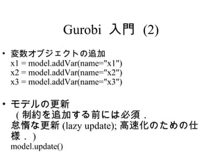
Gurobi 入門 (2)
• 変数オブジェクトの追加
x1 = model.addVar(name="x1")

• モデルの更新
( 制約を追加する前には必須．
怠惰な更新 (lazy update); 高速化のための仕
様． )
model.update()

Gurobi 入門 (3)
• 目的関数の設定
model.setObjective(15*x1 + 18*x2 + 30*x3,
GRB.MAXIMIZE)
• 制約の追加
model.addConstr(2*x1 + x2 + x3 <= 60)
model.addConstr(x1 + 2*x2 + x3 <= 60)
model.addConstr(x3 <= 30)
• 最適化
model.optimize()

リストを用いたモデル化
• 変数オブジェクトをリストに追加
x=[ 　 ]
for i in range(1,4):
var=model.addVar(name=“x[%s]”%i)
x.append(var)
• 制約 “ x1 + x2 + x3 <= 2” の追加
model.addConstr( sum(x) <= 2 ) or
model.addConstr( quicksum(x) <= 2 )

X[1] X[2] X[3] ・・・

辞書を用いたモデル化 (1)
• 辞書（ Dictionary ）は，ワインの種類
（“ Dry”, “Medium”, “Sweet”) をキーとし，
変数オブジェクトを値とした写像型
x={ }
x[“Dry”]= model.addVar(name=“Dry”)
x[“Medium”]= model.addVar(name=“Medium”)
x[“Sweet”]= model.addVar(name=“Sweet”)
値
キー
写 “ ニーハオ”
“Hello”,
Variable Object
“Dry 　
Wine”

辞書を用いたモデル化 (2)
• 制約 “ 2 x1 + x2 + x3 <= 30” の追加
model.addConstr( 2*x[“Dry”]+ x[“Medium”]
+x[“Sweet”] <=30 )

Blends, Profit =
multidict({"Dry":15, "Medium":18, "Sweet":30})
multidict

=> Blends=["Dry", "Medium“, "Sweet“]
Profit[“Dry”]=15, Profit[“Medium”]=18, ...

辞書を用いたワイン製造モデル
(1)
Blends, Profit =
multidict({"Dry":15, "Medium":18, "Sweet":30})
multidict

=> Blends=["Dry", "Medium“, "Sweet“] List of Keys
Profit[“Dry”]=15, Profit[“Medium”]=18, ...

Grapes, Inventory =
multidict({"Alfrocheiro":60, "Baga":60, "Castelao":30})

Use = { ("Alfrocheiro","Dry"):2, ("Alfrocheiro","Medium"):1,
("Alfrocheiro","Sweet"):1, ("Baga","Dry"):1, ....
}

辞書を用いたワイン製造モデル (2)
x = {}
for j in Blends:
x[j] = model.addVar(vtype="C", name="x[%s]"%j)
model.update()

model.setObjective(quicksum(Profit[j]*x[j] for j in Blends),
GRB.MAXIMIZE)
for i in Grapes:
model.addConstr(quicksum(Use[i,j]*x[j] for j in Blends)
<= Inventory[i], name="use[%s]"%i)

model.optimize()

k-median 問題
• min-sum 型の施設配置問題
• 顧客数 n=200 ，施設数 k=20
（顧客上から選択）
• Euclid 距離， x,y 座標は一様ランダム

n=200, k=5 の例

定式化

弱い定式化

Python での実装（ 1 ）
from gurobipy import * #gurobipy モジュールの読み込み

# k-median ソルバーの関数
def solve(n,k,cost):
model=Model(“median”) # モデルオブジェクトの生成
y={} # 変数を表す辞書の準備
x={}

キー値
“Hanako”, 写像 “127cm”
(1,2) 変数オブジェクト

Python での実装（２）
変数オブジェクトの追加
I=range(n) “B” は 0-1 整数 (binary) 変数
J=range(n) （ GRB.BINARY でも良い）
for j in J:
y[j] = model.addVar(vtype="B", name="y[%s]"%j)
for i in I:
x[i,j] =model.addVar( vtype="B",name="x[%s,%s]"%(i,j))
model.update()

目的関数の設定
model.setObjective(quicksum(c[i,j]*x[i,j] for i in I for j in J))

Python での実装（３）
for i in I:
model.addConstr(quicksum(x[i,j] for j in J) = = 1, "Assign[%s]"%i)

for j in J:
model.addConstr(x[i,j] <= y[j], "Strong[%s,%s]"%(i,j))

model.addConstr(quicksum(y[j] for j in J) = = k, "k_median")

Python での実装（４）
…
model.optimize()
print “Opt.value=”,model.ObjVal
edge=[]
for (i,j) in x:
if x[i,j].X= =1:
edge.append((i,j))
return edge

Python での実装（５）
import networkx as NX #networkX module
import matplotlib.pyplot as P #prepare drawing
P.ion()
G = NX.Graph() #graph object
G.add_nodes_from(range(n)) #add nodes
for (i,j) in edge: #add edges
G.add_edge(i,j)
NX.draw(G)

弱い定式化での結果
n=200,k=20
Optimize a model with 401 Rows, 40200 Columns and 80400
NonZeros
中略
Explored 1445 nodes (63581 simplex iterations) in 67.08 seconds
Thread count was 2 (of 2 available processors)
Optimal solution found (tolerance 1.00e-04)
Best objective 1.0180195861e+01, best bound 1.0179189780e+01,
gap 0.0099%
Opt.value= 10.1801958607

上界と下界の変化
18

16

14
Obj. Func . Va lue

12

10

8

6

4

2

0
0 10 20 30 40 50 60 70

CPU

強い定式化での結果
NonZeros
中略
( 分枝しないで終了！）
Thread count was 2 (of 2 available processors)
Best objective 1.0180195861e+01, best bound 1.0180195861e+01,
gap 0.0%
Opt.value= 10.1801958607

知見
• Big M を用いない強い定式化が望まし
い．
• この程度の式なら，必要な式のみを切
除平面として追加するような小細工は
必要なし．

（ただし，式の数が増え退化するので
，大規模なＬＰを高速に解けるソル
バーが前提）

k-center 問題
• min-max 型の施設配置問題
• 100 顧客， 10 施設（顧客上から選択）
• Euclid 距離， x,y 座標は一様ランダム

k-center (n=30,k=3) k-median (n=30,k=3)

1.2

1

0.8
Obj. Fun. Va lue

0.6

0.4

0.2

0
0 50 100 150 200 250 300 350 400

CPU Time

k- 被覆問題
距離が θ 以内の ( 被覆されている）顧客数

=1 顧客 i が被覆されている

パラメータ： =1
顧客 i から施設 j
への距離が θ 以
下

k- 被覆 + 二分探索

上界と下界 : UB ， LB
while UB – LB >ε:
θ= (UB+LB)/2
if k- 被覆問題の目的関数値が 0 then
UB = θ
else
LB = θ

知見
• Min-max 型の目的関数は MIP ソルバーでは解
きにくい（双対ギャップが大きい；上界も下
界も悪いので，途中で止めても悪い解！）．
• 例： Job shop スケジューリングの最大完了時
刻（メイクスパン）最小化
• k- 被覆問題として制約をなるべく満たすタイ
プのモデルに直して，最適値を二分探索する
とうまくいく．

巡回セールスマン問題（ＴＳ
Ｐ）
• すべての点をちょうど１回通る最短巡
回路
• 切除平面法で 85,900 点の実際問題（対
称ＴＳＰ）の最適解

Miller-Tucker-Zemlin の定式化

AMPL での実装（１）
param n >=0;
set V := 1..n ; # 点集合
set V0 := 2..n; # 出発地点 1 以外の点集合
set A :=V cross V; # 枝集合 = 点集合の直積（ 2 つ組）
param c { A } >= 0; # 枝の距離
var x { A } binary ; # 枝を使うとき 1 ，それ以外のとき 0 の 0-1 変
数
var u { V0 } >=1,<=n-1; # 点のポテンシャル
minimize total_cost:
sum {(i,j) in A} c[i,j] * x[i,j];

AMPL での実装（２）
Degree1 {i in V}:
sum {(i,j) in A } x[i,j] =1 ; # 出次数制約
Degree2 {i in V}:
sum {(j,i) in A } x[j,i] =1 ; # 入次数制約
MTZ{ (i,j) in A: i != j and j!=1 and i!=1}:
u[i]+1 -(n-1)*(1-x[i,j]) + (n-3)*x[j,i]<=u[j]; # 持ち上げ MTZ 制約
LiftedLB{ i in V0}:
1+(1-x[1,i]) +(n-3)*x[i,1] <= u[i]; # 持ち上げ下界制約
LiftedUB{ i in V0}:
u[i] <=(n-1)-(1-x[i,1])-(n-3)*x[1,i]; # 持ち上げ上界制約

45
（８０点， Euclid TSP ）
40

強化した式
35

30 でないと．．．
１日まわして
Obj. Func . Va lue

25

Out of Memory!
20

15

10

5

0
0 50 100 150 200 250 300 350 400

C PU

結果
Optimize a model with 6480 Rows, 6400 Columns and 37762 NonZeros
中略
Cutting planes:
Gomory: 62
Implied bound: 470
MIR: 299
Zero half: 34
Best objective 7.4532855108e+00, best bound 7.4525704995e+00, gap 0.0096%
Opt.value= 7.45328551084

知見
• 式を持ち上げ操作などで強化すると，
高速化され，大きな問題例が解けるよ
うになる．
　（そのためには多面体論の知識が多少
必要なので，専門家に相談する）

多品目ロットサイズ決定問題
• 段取り費用と在庫費用のトレードオフ
を最適化する多期間生産計画
• 多品目で共通の資源を使う容量制約付
き問題は， MIP ソルバーには難問（と
言われてきた）
• T=30 期， P=24 品目： Trigeiro, Thomas,
McClain （ 1989 年）の最大のベンチ
マーク

ロットサイズ決定問題
標準定式化のフローモデル
生産量 (t)

在庫量 (t-1) 在庫量 (t)
期
t

需要量 (t)
弱い定式化の原因

生産量 (t)≦ 大きな数 “ Large M” × 段取りの有無 (t)
在庫量（ t-1)+ 生産量 (t)= 需要量 (t)+ 在庫量（ t) 0-1 変数

ロットサイズ決定問題
施設配置定式化のフローモデル
s 期に生産して t 期まで在庫される量

期期
s t

需要量 (t)

s 期に生産して t 期まで在庫される量 ≦需要量 (t)× 段取りの有無 (s)

∑期に生産して t 期まで在庫される量 = 需要量 (t)
s
s ≤t

アルゴリズムと定式化の関係

（特殊形に対する）強い定式化 or
多項式時間アルゴリズム多項式時間で破っている
妥当不等式の同定

追加制約＋つなぎ制約

容量制約なしロットサイズ決定施設配置定式化
Wagner-Whitin 最短路定式化
動的計画アルゴリズム
(S,l) 不等式
１機械重み付き完了
時刻和最小化スケジューリング Super-modular 不等式
どん欲解法（ Simth’s rule ）

定式化のサイズと強さの比較
標準定式化施設配置定式化
変数の数 O(n) 変数の数
2
O(n )
制約の数
弱い定式化強い定式化
O(n) 制約の数
2
追加した
O(n ) = 線形計画緩和が
(S,l) 不等式整数多面体と一致
制約の数
O(2 n ) 切除平面
n: 期数
強い定式化

上界と下界の変化（標準定式
化） 1 32000

1 30000

1 28000

1 26000
Ob j. Fu n c . Va lu e

1 24000

1 22000

1 20000

1 18000

1 16000

1 14000

1 12000
0 200 400 600 800 1000 1200 1400 1600 1800 2000

C PU

1800 秒で最適解；これ以上大きな問題例は無理！

上界と下界の変化（施設配置定式
1 14050
化）
1 14000

1 13950
Ob j. Fu n c . Va l.

1 13900

1 13850

1 13800

1 13750

1 13700

1 13650

1 13600
0 5 10 15 20 25 30 35 40 45

C PU

40 秒で最適解； T=100 でも大丈夫！

知見
• 従来では難問と言われてきたロットサ
イズ決定問題でもある程度までは大丈
夫
• 緩和固定法（ Federgruen, Meissner,Tzur
“Progressive Interval Heuristics for Multi-
Item Capacitated Lot-Sizing Problems”
2007 ）という MIP ベースのメタ解法を
作ってみたが，同時間通常の探索を行
う「打ち切り分枝限定法」の方が良
い！

グラフ彩色問題
• 解の対称性
• 点数 n=40 ，彩色数上限 Kmax=10
• ランダムグラフ G(n,p=0.5)
• 彩色数 8 が最適値

Python での実装（１）
from gurobipy import *
model=Model("gcp")
x={}
y={}
for i in range(n):
for k in range(K):
x[i,k]=model.addVar(obj=0, vtype="B",name="x"+str(i)+str(k))
for k in range(K):
y[k]=model.addVar(obj=1,vtype=“B”,name="y"+str(k))
model.update()

Python での実装（２）
for i in range(n):
L=LinExpr()
for k in range(K):
L.addTerms(1,x[i,k])
　　　 model.addConstr(lhs=L,sense= " = ",rhs=1,name="const"+str(i))
中略
model.optimize()
print "Opt.value=",model.ObjVal
for v in model.getVars():
if v.X>0.001:
print v.VarName,v.X

上界と下界の変化（原定式
化）
12
点数 n=40 ，彩色数上限 Kmax=10
10
Obj. Func . Value

8

6

4

2

0
0 200 400 600 800 1000 1200 1400

CPU Time

定式化の改良
対称性の除去（番号の小さい方の色を優先して使う！）

特殊順序集合（ SOS: Special Ordered Set ） Type 1 （いずれか
１つの変数が正になることの宣言）の追加

model.addSOS(1, 変数リス
ト)

上界と下界の変化（対称性除
12
去）
10
Obj. Func . Va lue

8

6

4

2

0
0 50 1 00 1 50 200 250 300 350 400 450

CPU
MIPFocus=2 （最適性保証優先）で 67 秒， MIPFocus=3 （下界優先）で

上界と下界の変化（ +SOS ）
12

10
Obj. Func . Va l.

8

6

4

2

0
0 5 10 15 20 25

CPU
NonZerosExplored 109 nodes (58792 simplex iterations) in 22.02 seconds
MIPFocus=2 （最適性保証優先）で 65 秒， MIPFocus=3 （下界優先）
で 126 秒

知見
• 解の対称性のある問題は，下界の改善がしに
くいので，分枝限定法では解きにくい（モダ
ンなソルバーは群論などを用いた工夫を入れ
てはいるが，あまり機能しない問題もある）
• 対称性を除く工夫を入れると多少は改善
• SOS （ Special Ordered Set ）制約の宣言は損
はない（ただし，探索手法の変更との相性は
悪い．）

Gurobi クラス
• モデルクラス Model
モデルオブジェクト =Model(“ モデル名”）
• 変数クラス Var
変数オブジェクト = モデルオブジェクト .addVar()
• 制約クラス Constr
制約オブジェクト = モデルオブジェク
ト .addConstr()
• 線形制約クラス LinExpr
線形制約オブジェクト =LinExpr()
• 他にも，特殊順序集合クラス SOS ，定数クラス
GRB ，コールバッククラス Callbacks ，エラークラ
ス GurobiError ，列クラス Column がある．

Gurobi Objects
GRBError
Variable
addVar

Model Column

addSOS addConstr
Constraint
SOS

Callbacks LinExpr QuadExpr

変数追加メソッド addVar の
引数
• lb ( 下限 ) ：規定値 =0
• ub ( 上限 ) ：規定値 =GRB.INFINITY （無限
大）
• obj ( 目的関数の係数 ) ：＝０
• vtype ( 変数の種類 ): GRB.CONTINUOUS （連
続変数； “ C” でも可） , GRB.BINARY （ 2 値
変数；“ B” ） , GRB.INTEGER （整数変
数；“ I” ） , GRB.SEMICONT （ 0 もしくはあ
る範囲内の連続変数；“ S” でも可） ,
GRB.SEMIINT （ 0 もしくはある範囲内の整
数変数；“ N” でも可）
• name ( 名前 ): =“”

制約追加メソッド addConstr の引
数
• ｌ hs （左辺）：線形制約オブジェク
トか定数
• sense （制約の向き）：
GRB.LESS_EQUAL （≦；“ <” でも可） ,
GRB.EQUAL （＝； “ =” でも可） ,
GRB.GREATER_EQUAL （≧；“ >” でも
可）
• rhs （右辺）：線形制約オブジェクトか
定数

モデルのその他の主要メソッ
ド
• optimize( コールバック関数）：最適化実行
• update ：モデルの変更を Gurobi に知らせる
• getVars ：変数オブジェクトを入れたリスト
を得る
• relax ：緩和問題を生成
• computeIIS ：既約不整合部分系（実行不能に
なっている原因の制約と変数； Irreducible
Inconsistent Subsystem ： IIS ）を計算
• addSOS （ 1 or 2, 変数リスト，重み
（ option ））：特殊順序集合（ Special
Ordered Set ： SOS ）を追加

パラメータの設定
書式：
setParam(“ パラメータ名” , 値）
model.Params. パラメータ名 = 値
例：混合整数計画（ MIP ）の相対誤差
（終了条件）；規定値は 10-4
setParam(“MIPGap”,0.0)
model.Params.MIPGap=0.0

よく使うパラメータ
• TimeLimit ：計算時間上限（秒）
• MIPGap ：相対誤差上限（規定値は 10-4 ）
• MIPFocus ： MIP 探索戦略（ 0= バランス ,1=
暫定解改良 ,2= 最適性の保証 ,3= 限界値改
良）
• SolutionNumber ：探索中に発見された解の番
号
• LPMethod ：線形計画の解法（ 0= 主単体， 1=
双対単体， 2= 内点）
• OutputFlag ：出力制御（ 0=Off ， 1=On ）

属性（ attributes ）
書式：
オブジェクト .setAttr(“ 属性名” , 値）
オブジェクト . 属性名 = 値
例：変数 var の目的関数の係数を 100 に
変更
var.setAttr(“Obj”,100)
var.Obj=100

よく使う属性（ 1 ）
• モデル
– ObjVal ：最適目的関数値（最適化後のみ）
– ModelSense ：目的関数の方向（ 1= 最小化， -1= 最
大化）
– Runtime ：計算時間（最後の求解時の）
– Status ：モデルの状態（１から 1 ３まで；
2=OPTIMAL, 3=INFEASIBLE, 4=UNBOUNDED,
9=TIME_LIMIT, 11=INTERRUPTED,
13=SUBOPTIMAL)
– SolCount ：探索で見つかった解の数

よく使う属性（２）
• 変数
– LB ， UB ：下限，上限
– Obj ：目的関数の係数
– Vtype ：変数の種類（“ C”= 連続，“ B”=2 値，“ I”= 整数，“ S” ＝半連続
，“ N”= 半整数
– VarName ：変数名
– X ：解の値
– Xn ：パラメータ SolutionNumber で指定された番号の解の値
– RC ：被約費用（連続最適化のみ）
• 制約
– Sense ：制約の向き（“ <” ，“ >” ，“ =” ）
– RHS ：右辺定数
– ConstrName ：制約名
– Pi ：双対変数（連続最適化のみ）
– Slack ：余裕変数の値

Gurobi python

Recommended

More Related Content

What's hot (20)

Viewers also liked (20)

Similar to Gurobi python (20)

More from Mikio Kubo (9)

Gurobi python

Editor's Notes