


![X, Y be topological spaces, and f, g : X → Y
continuous maps. A Homotopy from f to g is a
continuous function F : X × [0, 1] → Y satisfying
F(x, 0) = f(x) and F(x, 1) = g(x), for all x ∈ X.
The two dashed paths shown above
are homotopic relative to their
endpoints. The animation represents
one possible homotopy
HOMOTOPY
Introduced by
Professor JH He](https://image.slidesharecdn.com/extensionofhomotopyfinal-220730151601-8a0b5d05/85/Homotopy-Perturbation-Method-7-320.jpg)


![Construct a Homotopy
𝐻 𝑣, 𝑝 = 1 − 𝑝 𝐿 𝑣 − 𝐿 𝑢0 + 𝑝 𝐴 𝑣 − 𝑓 𝑟 = 0,where𝑣 ∶ Ω × 0, 1 → ℝ
𝑝 ∈ [0, 1] = embedding parameter
𝑢0 = first approximation , satisfies the boundary conditions.
Satisfies
𝐻 𝑣, 0 = 𝐿 𝑣 − 𝐿 𝑢0 = 0
𝐻 𝑣, 1 = 𝐿 𝑢 + 𝑁 𝑢 − 𝑓 𝑟 = 0
written as a power series in p, as following:
𝑣 = 𝑣0 + 𝑝𝑣1 + 𝑝2 𝑣2 + ⋯
If set 𝑝 = 1
The best approximation is:
𝑢 = lim
𝑝→1
𝑣 = 𝑣0 + 𝑣1 + 𝑣2 + …](https://image.slidesharecdn.com/extensionofhomotopyfinal-220730151601-8a0b5d05/85/Homotopy-Perturbation-Method-11-320.jpg)
![Solving Laplace Equationby Separation
of Variable Method
𝐿𝑎𝑝𝑙𝑎𝑐𝑒 𝐸𝑞𝑢𝑎𝑡𝑖𝑜𝑛
𝜕2𝑢
𝜕𝑥2
+
𝜕2𝑢
𝜕𝑦2
= 0 , u is the temperature
by separation of variable method
𝑢 𝑥, 𝑦 = 𝑋 𝑥 . 𝑌(𝑦) ..……………….. (ii)
[Where X is the function x only and Y is a function of y only.]
Now, differentiating partially with respect to x and y we get,
𝜕2𝑢
𝜕𝑥2 = 𝑌
𝑑2𝑋
𝑑𝑥2 and
𝜕2𝑢
𝜕𝑦2 = 𝑋
𝑑2𝑌
𝑑𝑦2 ……………………. (iii)
Now using equation (iii) into equation (i),
𝑌
𝑑2𝑋
𝑑𝑥2 + 𝑋
𝑑2𝑌
𝑑𝑦2 = 0 Or,
1
𝑋
𝑑2𝑋
𝑑𝑥2 = −
1
𝑌
𝑑2𝑌
𝑑𝑦2 = 𝑘 (say) ……………………... (iv)](https://image.slidesharecdn.com/extensionofhomotopyfinal-220730151601-8a0b5d05/85/Homotopy-Perturbation-Method-12-320.jpg)


![Now the initial conditions are
𝑢(0, 𝑦) = 𝑥𝑓(𝑦)
𝑢𝑥(0, 𝑦) = 𝑓1(𝑦)
From (ii) we get
𝑢𝑥 = ℎ 𝑦 = 𝑓1(𝑦)
From (iii) we get ,
𝑈(0, 𝑦) = 𝑥𝑓(𝑦) = 𝑔(𝑦)
Now
𝑢0 = 𝑥ℎ(𝑦) + 𝑔(𝑦)
= [𝑥𝑓1(𝑦) + 𝑥𝑓(𝑦)]](https://image.slidesharecdn.com/extensionofhomotopyfinal-220730151601-8a0b5d05/85/Homotopy-Perturbation-Method-17-320.jpg)
![𝑝(1)
∶ 𝑢1 𝑥, 𝑦 = −
𝑥3
6
[𝑓1
2
y + 𝑓2
𝑦 ] + 𝑢0
Similarly ,
𝑝(2)
∶ 𝑢2 𝑥, 𝑦 =
𝑥6
720
[𝑓1
4
y + 𝑓4
𝑦 ] +
𝑥2
2
[𝑓1
2
y + 𝑓2
𝑦 ] + 𝑢0
⋮
⋮
𝐺𝑖𝑣𝑒𝑠 𝑡ℎ𝑒 𝑠𝑜𝑙𝑢𝑡𝑖𝑜𝑛 𝑎𝑠 ,
𝑢 = 𝑛𝑢0 − −1 𝑛+1
𝑥3𝑛
3𝑛 !
+
𝑥2𝑛
2𝑛 !
∙ [𝑓1
3𝑛−2
(𝑦) + 𝑓 3𝑛−2
(𝑦)]
𝑊ℎ𝑒𝑟𝑒 𝑛 𝑖𝑠 𝑡ℎ𝑒 𝑛𝑢𝑚𝑏𝑒𝑟 𝑜𝑓 𝑝𝑒𝑟𝑡𝑢𝑟𝑏𝑎𝑡𝑖𝑜𝑛 , 𝑎𝑛𝑑 𝑛𝜖ℕ](https://image.slidesharecdn.com/extensionofhomotopyfinal-220730151601-8a0b5d05/85/Homotopy-Perturbation-Method-18-320.jpg)
![EXAMPLE:
If we consider the Laplace equation
𝛻2 =
𝜕2
𝑢
𝜕𝑥2
+
𝜕2
𝑢
𝜕𝑦2
= 0 , 𝑤ℎ𝑒𝑟𝑒 𝑢 𝑖𝑠 𝑡ℎ𝑒 𝑡𝑒𝑚𝑝𝑒𝑟𝑎𝑡𝑢𝑟𝑒,
u=u(x,y)
Substituting the equation by Homotopy Perturbation method ,
We get,
𝐻(𝑥, 𝑦, 𝑝) = (1 − 𝑝)[
𝜕2𝑢(𝑥,𝑦)
𝜕𝑥2 ] + p[
𝜕2𝑢(𝑥,𝑦)
𝜕𝑥2 +
𝜕2𝑢(𝑥,𝑦)
𝜕𝑦2 ] = 0 … ………(ii)
Consider U(x,y) as
U(x,y) = 𝑢0 (𝑥, 𝑦) + 𝑃𝑈1(𝑥, 𝑦) + 𝑃2
𝑈2(𝑥, 𝑦) + … + ………(iii)
Substituting Eq(iii) into Eq(ii) and rearranging based on power p-terms we have,
𝑝(0) ∶
𝜕2
𝑢(𝑥, 𝑦)
𝜕𝑥2
= 0
Initial condition
𝑢0 0, 𝑦 = 0
𝑢0 𝜋, 𝑦 = sinh(𝑦) cos(𝑦)
𝑢 𝑥, 0 = sinh(𝑥)
𝑢0 𝑥, 𝜋 = −sinh(𝑥)](https://image.slidesharecdn.com/extensionofhomotopyfinal-220730151601-8a0b5d05/85/Homotopy-Perturbation-Method-19-320.jpg)


![REFERENCES
[1] A. Belendez, A. Hernandez, T. Belendez et al., Application of He’s Homotopy
perturbation method to the Duffing-harmonic oscillator, Internat. J. Nonlinear Sci. 8
(2007), 79–88.
[2] M. Matinfar and M. Ghanbari, “Homotopy Perturbation Method for the Fisher’s
Equation and It’s Generalized,” International Journal of Nonlinear Science, Vol. 8, No. 4,
2009, pp. 448-455.
[3] P. Roul, “Application of Homotopy Perturbation Method to Biological Population
Model,” Applications and Applied Mathematics: An International Journal, Vol. 5, No. 10,
2010, pp. 13969-1378
[4] M. Ghasemi, M. T. Kajani and E. Babolian, “Application of He’S Homotopy Perturbation
Method to Nonlinear Integro-Differential Equations,” Applied Mathematics and
Computation, Vol. 188, No. 1, 2007, pp. 538-548
[5] He, J. H. (1999a). Homotopy-perturbation technique, Comput. Methods Appl. Mech.
Engrg. 178, pp. 257-262.
[6] He, J. H. (1999b). Variational iteration method: a kind of nonlinear analytical technique:
Some examples, International Journal of Nonlinear Mechanics, 344, pp. 699-708.](https://image.slidesharecdn.com/extensionofhomotopyfinal-220730151601-8a0b5d05/85/Homotopy-Perturbation-Method-25-320.jpg)


Homotopy Perturbation Method
- 1. In
- 2. Submitted by- Murshiul Habib Khandakar , Aparna Purkait , Rinku Alam , Soumya Das and Ruksena Parvin Supervised by- Dr. Banashree Sen in partial fulfillment for the award of the degree of Master of Science Applied Mathematics, Academic Year: 2021-22 Department of Applied Mathematics , School of Applied Science and Technology, Maulana Abul Kalam Azad University of Technology (formerly WBUT) Haringhata, Dist- Nadia, West Bengal, India, PIN- 741239
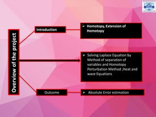
- 3. Overview of the project Introduction Homotopy, Extension of Homotopy Outcome Solving Laplace Equation by Method of separation of variables and Homotopy Perturbation Method ;Heat and wave Equations Absolute Error estimation
- 4. Second order partial differential equation Laplace Equation: (Two Dimensional) It’s states that the sum of the 2nd order partial derivatives of U ,the unknown function ,with respect to the Cartesian coordinates, equals zero. 𝜕2 𝑢 𝜕𝑥2 + 𝜕2 𝑢 𝜕𝑦2 = 0 , u is the temperature
- 5. Wave Equation: It’s describes the propogation of oscillations at a fixed speed in some quantity y : 𝜕2 𝑢 𝜕𝑥2 = 1 𝐶2 𝜕2 𝑢 𝜕𝑇2 Heat Equation: (One Dimensional) It’s describe the distribution of heat in a given space over time 𝜕𝑢 𝜕𝑡 =k 𝜕2𝑢 𝜕𝑥2
- 6. Methods for solving Laplace equation Homotopy Perturbation Method Method of separation variable
- 7. X, Y be topological spaces, and f, g : X → Y continuous maps. A Homotopy from f to g is a continuous function F : X × [0, 1] → Y satisfying F(x, 0) = f(x) and F(x, 1) = g(x), for all x ∈ X. The two dashed paths shown above are homotopic relative to their endpoints. The animation represents one possible homotopy HOMOTOPY Introduced by Professor JH He
- 8. Uses of Homotopy Perturbation Method Population balance Fractor Toda Oscillator Parameter expansion technology Nanofluid technology
- 9. WHY WE PREFER HOMOTOPY PERTURBATION METHOD ? This is relatively a new technic and easy to handle for solving linear and non-linear partial differential equation. It is simple method compare to another iterative method. For solving this method we get nearest value of exact solution than another method. Error is more less than other method.
- 10. The Homotopy Perturbation Method: we consider the following equation 𝐴 𝑢 − 𝑓 𝑟 = 0, 𝑟 ∈ Ω ………………………………….(Equation.1) with the boundary condition: 𝐵 𝑢, 𝜕𝑢 𝜕𝑛 = 0 , 𝑟∈ Γ, A = general differential operator, B =boundary operator, 𝑓 𝑟 = analytical function G = boundary of the domain Ω. A = L + N, L is linear and N is nonlinear. 𝐿 𝑢 + 𝑁 𝑢 − 𝑓 𝑟 = 0, 𝑟 ∈ Ω ……………………(Equation.2)
- 11. Construct a Homotopy 𝐻 𝑣, 𝑝 = 1 − 𝑝 𝐿 𝑣 − 𝐿 𝑢0 + 𝑝 𝐴 𝑣 − 𝑓 𝑟 = 0,where𝑣 ∶ Ω × 0, 1 → ℝ 𝑝 ∈ [0, 1] = embedding parameter 𝑢0 = first approximation , satisfies the boundary conditions. Satisfies 𝐻 𝑣, 0 = 𝐿 𝑣 − 𝐿 𝑢0 = 0 𝐻 𝑣, 1 = 𝐿 𝑢 + 𝑁 𝑢 − 𝑓 𝑟 = 0 written as a power series in p, as following: 𝑣 = 𝑣0 + 𝑝𝑣1 + 𝑝2 𝑣2 + ⋯ If set 𝑝 = 1 The best approximation is: 𝑢 = lim 𝑝→1 𝑣 = 𝑣0 + 𝑣1 + 𝑣2 + …
- 12. Solving Laplace Equationby Separation of Variable Method 𝐿𝑎𝑝𝑙𝑎𝑐𝑒 𝐸𝑞𝑢𝑎𝑡𝑖𝑜𝑛 𝜕2𝑢 𝜕𝑥2 + 𝜕2𝑢 𝜕𝑦2 = 0 , u is the temperature by separation of variable method 𝑢 𝑥, 𝑦 = 𝑋 𝑥 . 𝑌(𝑦) ..……………….. (ii) [Where X is the function x only and Y is a function of y only.] Now, differentiating partially with respect to x and y we get, 𝜕2𝑢 𝜕𝑥2 = 𝑌 𝑑2𝑋 𝑑𝑥2 and 𝜕2𝑢 𝜕𝑦2 = 𝑋 𝑑2𝑌 𝑑𝑦2 ……………………. (iii) Now using equation (iii) into equation (i), 𝑌 𝑑2𝑋 𝑑𝑥2 + 𝑋 𝑑2𝑌 𝑑𝑦2 = 0 Or, 1 𝑋 𝑑2𝑋 𝑑𝑥2 = − 1 𝑌 𝑑2𝑌 𝑑𝑦2 = 𝑘 (say) ……………………... (iv)
- 13. 𝑑2𝑋 𝑑𝑥2 − 𝑘𝑥 = 0 ………………….. (v) 𝑑2𝑌 𝑑𝑦2 + 𝑘𝑦 = 0 …………………... (vi) Equation (v) and (vi) are second order ODE and there are three cases which depend on k. Case: 1 If 𝑘 = 𝜆2 ≥ 0 The required solution is, 𝑢 𝑥, 𝑦 = 𝐴 𝑒𝜆𝑥 + 𝐵 𝑒−𝜆𝑥 + (𝐶 cos 𝜆𝑦 + 𝐷 sin 𝜆𝑦) 𝑑2𝑋 𝑑𝑥2 − 𝜆2 𝑥 = 0 Or, 𝐷2 − 𝜆2 𝑋 = 0 A.E ; 𝑚2 − 𝜆2 = 0 Or, 𝑚 = ±𝜆 Required solution, 𝑋 = 𝐴 𝑒𝜆𝑥 + 𝐵 𝑒−𝜆𝑥 𝑑2𝑌 𝑑𝑦2 + 𝜆2 𝑦 = 0 Or, 𝐷2 + 𝜆2 𝑌 = 0 A.E ; 𝑚2 + 𝜆2 = 0 Or, 𝑚 = ±𝜆𝑖 Required solution, 𝑌 = 𝐶 cos 𝜆𝑦 + 𝐷 sin 𝜆𝑦
- 14. Case: 2 If 𝑘 = −𝜆2 ≤ 0 The required solution is, 𝑢 𝑥, 𝑦 = 𝐴 cos 𝜆𝑥 + 𝐵 sin 𝜆𝑥 + (𝐶 𝑒𝜆𝑦 + 𝐷 𝑒−𝜆𝑦) 𝑑2𝑋 𝑑𝑥2 + 𝜆2 𝑥 = 0 Or, 𝐷2 + 𝜆2 𝑋 = 0 A.E ; 𝑚2 + 𝜆2 = 0 Or, 𝑚 = ±𝜆𝑖 Required solution, 𝑋 = 𝐴 cos 𝜆𝑥 + 𝐵 sin 𝜆𝑥 𝑑2𝑌 𝑑𝑦2 − 𝜆2 𝑦 = 0 Or, 𝐷2 − 𝜆2 𝑌 = 0 A.E ; 𝑚2 − 𝜆2 = 0 Or, 𝑚 = ±𝜆 Required solution, 𝑌 = 𝐶 𝑒𝜆𝑦 + 𝐷 𝑒−𝜆𝑦
- 15. 𝐶𝑜𝑛𝑠𝑖𝑑𝑒𝑟 𝑡ℎ𝑒 𝐿𝑎𝑝𝑙𝑎𝑐𝑒 𝐸𝑞𝑢𝑎𝑡𝑖𝑜𝑛 𝜕2 𝑢 𝜕𝑥2 + 𝜕2 𝑢 𝜕𝑦2 = 0 , u is the temperature 𝑊𝑖𝑡ℎ 𝑖𝑛𝑖𝑡𝑖𝑎𝑙 𝑐𝑜𝑛𝑑𝑖𝑡𝑖𝑜𝑛𝑠 𝑢 0, 𝑦 = 𝑥𝑓 𝑦 , 𝑢 𝑥, 0 = 0 , 𝑢𝑥 0, 𝑦 = 𝑓1 𝑦 𝑢 = 𝑓 𝑦 𝑅 𝑥 𝑢 = 0 𝑢 = 0 𝑢 = 0 0 0
- 16. 𝐴𝑝𝑝𝑙𝑦𝑖𝑛𝑔 𝑡ℎ𝑒 𝑐𝑜𝑛𝑣𝑒𝑥 ℎ𝑜𝑚𝑜𝑡𝑜𝑝𝑦 𝑚𝑒𝑡ℎ𝑜𝑑𝑠 , 𝑊𝑒 𝑔𝑒𝑡 𝜕2 𝜕𝑥2 𝑢0 + p𝑢1 + 𝑝2 𝑢2 + 𝑝3 𝑢3 + ⋯ + p 𝜕2 𝜕𝑦2 𝑢0 + p𝑢1 + 𝑝2 𝑢2 + 𝑝3 𝑢3 + ⋯ = 0 𝑁𝑜𝑤 𝑐𝑜𝑚𝑝𝑎𝑟𝑖𝑛𝑔 𝑡ℎ𝑒 𝑐𝑜𝑒𝑓𝑓𝑐𝑖𝑒𝑛𝑡𝑠 𝑜𝑓 𝑒𝑞𝑢𝑎𝑙 𝑝𝑜𝑤𝑒𝑟 𝑜𝑓 𝑝 We get , 𝜕2𝑢0 𝜕𝑥2 = 0 …………………(i) Integrating (i) with respect to x , keeping y as a constant , 𝜕𝑢0 𝜕𝑥 = h(y)…………(ii) Again Intigrating (ii) with respect to x , keeping y as a constant , 𝑥0 = 𝑥ℎ 𝑦 + 𝑔(𝑦)…………..(iii)
- 17. Now the initial conditions are 𝑢(0, 𝑦) = 𝑥𝑓(𝑦) 𝑢𝑥(0, 𝑦) = 𝑓1(𝑦) From (ii) we get 𝑢𝑥 = ℎ 𝑦 = 𝑓1(𝑦) From (iii) we get , 𝑈(0, 𝑦) = 𝑥𝑓(𝑦) = 𝑔(𝑦) Now 𝑢0 = 𝑥ℎ(𝑦) + 𝑔(𝑦) = [𝑥𝑓1(𝑦) + 𝑥𝑓(𝑦)]
- 18. 𝑝(1) ∶ 𝑢1 𝑥, 𝑦 = − 𝑥3 6 [𝑓1 2 y + 𝑓2 𝑦 ] + 𝑢0 Similarly , 𝑝(2) ∶ 𝑢2 𝑥, 𝑦 = 𝑥6 720 [𝑓1 4 y + 𝑓4 𝑦 ] + 𝑥2 2 [𝑓1 2 y + 𝑓2 𝑦 ] + 𝑢0 ⋮ ⋮ 𝐺𝑖𝑣𝑒𝑠 𝑡ℎ𝑒 𝑠𝑜𝑙𝑢𝑡𝑖𝑜𝑛 𝑎𝑠 , 𝑢 = 𝑛𝑢0 − −1 𝑛+1 𝑥3𝑛 3𝑛 ! + 𝑥2𝑛 2𝑛 ! ∙ [𝑓1 3𝑛−2 (𝑦) + 𝑓 3𝑛−2 (𝑦)] 𝑊ℎ𝑒𝑟𝑒 𝑛 𝑖𝑠 𝑡ℎ𝑒 𝑛𝑢𝑚𝑏𝑒𝑟 𝑜𝑓 𝑝𝑒𝑟𝑡𝑢𝑟𝑏𝑎𝑡𝑖𝑜𝑛 , 𝑎𝑛𝑑 𝑛𝜖ℕ
- 19. EXAMPLE: If we consider the Laplace equation 𝛻2 = 𝜕2 𝑢 𝜕𝑥2 + 𝜕2 𝑢 𝜕𝑦2 = 0 , 𝑤ℎ𝑒𝑟𝑒 𝑢 𝑖𝑠 𝑡ℎ𝑒 𝑡𝑒𝑚𝑝𝑒𝑟𝑎𝑡𝑢𝑟𝑒, u=u(x,y) Substituting the equation by Homotopy Perturbation method , We get, 𝐻(𝑥, 𝑦, 𝑝) = (1 − 𝑝)[ 𝜕2𝑢(𝑥,𝑦) 𝜕𝑥2 ] + p[ 𝜕2𝑢(𝑥,𝑦) 𝜕𝑥2 + 𝜕2𝑢(𝑥,𝑦) 𝜕𝑦2 ] = 0 … ………(ii) Consider U(x,y) as U(x,y) = 𝑢0 (𝑥, 𝑦) + 𝑃𝑈1(𝑥, 𝑦) + 𝑃2 𝑈2(𝑥, 𝑦) + … + ………(iii) Substituting Eq(iii) into Eq(ii) and rearranging based on power p-terms we have, 𝑝(0) ∶ 𝜕2 𝑢(𝑥, 𝑦) 𝜕𝑥2 = 0 Initial condition 𝑢0 0, 𝑦 = 0 𝑢0 𝜋, 𝑦 = sinh(𝑦) cos(𝑦) 𝑢 𝑥, 0 = sinh(𝑥) 𝑢0 𝑥, 𝜋 = −sinh(𝑥)
- 20. 𝑝(1) ∶ 𝜕2 𝑢1(𝑥, 𝑦) 𝜕𝑥2 + 𝜕2 𝑢0(𝑥, 𝑦) 𝜕𝑦2 = 0 Initial condition 𝑢1 0, 𝑦 = 0 𝑢1 𝜋, 𝑦 = 0 𝑢1 𝑥, 𝑦 = 0 𝑢1 𝑥, 𝜋 = 0 𝑝2 : 𝜕2𝑢2(𝑥,𝑦) 𝜕𝑥2 + 𝜕2𝑢1(𝑥,𝑦) 𝜕𝑦2 = 0 𝑢2 0, 𝑦 = 0 𝑢2 𝜋, 𝑦 = 0 𝑢2 𝑥, 𝑦 = 0 𝑢2 𝑥, 𝜋 = 0 𝑝3 : 𝜕2𝑢3(𝑥,𝑦) 𝜕𝑥2 + 𝜕2𝑢3(𝑥,𝑦) 𝜕𝑦2 = 0𝑢2 0, 𝑦 = 0 𝑢2 𝜋, 𝑦 = 0 𝑢2 𝑥, 𝑦 = 0 𝑢2 𝑥, 𝜋 = 0
- 21. Solving equation(i) with boundary conditions 𝑢 𝑥, 𝑦 = 𝑥 𝑐𝑜𝑠𝑦 The zeroth approximation satisfies boundary condition 𝑢1 𝑥, 𝑦 = 1 3! 𝑥3𝑐𝑜𝑠𝑦 𝑢2 𝑥, 𝑦 = 1 5! 𝑥5𝑐𝑜𝑠𝑦 𝑢3 𝑥, 𝑦 = 1 7! 𝑥3𝑐𝑜𝑠𝑦 U(x,y) = cosy[x+ 𝑥3 3! + 𝑥5 5! + 𝑥3 7! + … =cosy sinhx =sinhx cosy
- 23. Conclusion We applied the HPM for finding the solution of a system of partialdifferential equations. The method is applied in a direct way without using linearization, transformation,discretization or restrictive assumptions. It may be concluded that the HPM is very powerful and efficientin finding the analytical solutions for a wide class y of boundary value problems. It is a semi analytic method. The method gives more realistic series solutions that converge very rapidly in physical problems. It is worth mentioning that the method is capable of reducing the volume of the computational work as compared to the classical methods while still maintaining the high accuracy of the numerical result.
- 24. Future scope This HPM is also well fitted for solving Differential equations. Through the approach in (The International Journal of Engineering and Science (IJES) || Volume || 8 || Issue || 12 || Series I || Pages || PP 28-35|| 2019 || ISSN (e): 2319 – 1813 ISSN (p): 23-19 – 1805), the HPM can be extended to solve ordinary differential equations. The method requires less work with very little cost (when compared with other numerical methods like classical RK).
- 25. REFERENCES [1] A. Belendez, A. Hernandez, T. Belendez et al., Application of He’s Homotopy perturbation method to the Duffing-harmonic oscillator, Internat. J. Nonlinear Sci. 8 (2007), 79–88. [2] M. Matinfar and M. Ghanbari, “Homotopy Perturbation Method for the Fisher’s Equation and It’s Generalized,” International Journal of Nonlinear Science, Vol. 8, No. 4, 2009, pp. 448-455. [3] P. Roul, “Application of Homotopy Perturbation Method to Biological Population Model,” Applications and Applied Mathematics: An International Journal, Vol. 5, No. 10, 2010, pp. 13969-1378 [4] M. Ghasemi, M. T. Kajani and E. Babolian, “Application of He’S Homotopy Perturbation Method to Nonlinear Integro-Differential Equations,” Applied Mathematics and Computation, Vol. 188, No. 1, 2007, pp. 538-548 [5] He, J. H. (1999a). Homotopy-perturbation technique, Comput. Methods Appl. Mech. Engrg. 178, pp. 257-262. [6] He, J. H. (1999b). Variational iteration method: a kind of nonlinear analytical technique: Some examples, International Journal of Nonlinear Mechanics, 344, pp. 699-708.
- 26. ACKNOWLEDGEMENT Primarily, we would like to thank our respected project guide Dr. Banashree Sen who gave us this opportunity to work on this project. We got to learn a lot from this project about “Extension of Homotopy Perturbation Methods in Laplace Equation, Heat Equation and Wave Equation.” Also, We are thankful to Maulana Abul Kalam Azad University of Technology (MAKAUT) for providing us MATLAB AND SIMULINK software access and this opportunity of Term-Project in the curriculum.