SlideShare a Scribd company logo
Course Program
9.30-10.00 Introduction (Andrew Blake)
10.00-11.00 Discrete Models in Computer Vision (Carsten Rother)
15min Coffee break
11.15-12.30 Message Passing: DP, TRW, LP relaxation (Pawan Kumar)
12.30-13.00 Quadratic pseudo-boolean optimization (Pushmeet Kohli)
1 hour Lunch break
14:00-15.00 Transformation and move-making methods (Pushmeet Kohli)
15:00-15.30 Speed and Efficiency (Pushmeet Kohli)
15min Coffee break
15:45-16.15 Comparison of Methods (Carsten Rother)
16:15-17.30 Recent Advances: Dual-decomposition, higher-order, etc.
             (Carsten Rother + Pawan Kumar)

   All online material will be online (after conference):
   http://research.microsoft.com/en-us/um/cambridge/projects/tutorial/
Comparison of Optimization Methods

             Carsten Rother
      Microsoft Research Cambridge
Why is good optimization important?


Input: Image sequence


                                                [Data courtesy from Oliver Woodford]


Output: New view


Problem: Minimize a binary 4-connected pair-wise MRF
         (choose a colour-mode at each pixel)
                                                     [Fitzgibbon et al. ‘03+
Why is good optimization important?


Ground Truth   Graph Cut with truncation    Belief Propagation             ICM, Simulated
               [Rother et al. ‘05+
                                                                           Annealing


                                           QPBOP [Boros ’06, Rother ‘07+
                                           Global Minimum
Comparison papers
• Binary, highly-connected MRFs *Rother et al. ‘07+


• Multi-label, 4-connected MRFs *Szeliski et al. ‘06,‘08+
  all online: http://vision.middlebury.edu/MRF/


• Multi-label, highly-connected MRFs *Kolmogorov et al. ‘06+
Comparison papers
• Binary, highly-connected MRFs *Rother et al. ‘07+


• Multi-label, 4-connected MRFs *Szeliski et al. ‘06,‘08+
  all online: http://vision.middlebury.edu/MRF/


• Multi-label, highly-connected MRFs *Kolmogorov et al. ‘06+
Random MRFs
o Three important factors:
   o Connectivity (av. degree of a node)
   o Unary strength: E(x) = w ∑ θi (xi) + ∑ θij (xi,xj)
   o Percentage of non-submodular terms (NS)
Computer Vision Problems

       perc. unlabeled (sec)   Energy   (sec)


Conclusions:
      • Connectivity is a crucial factor
       • Simple methods like Simulated
         Annealing sometimes best
Diagram Recognition [Szummer et al ‘04]
                      71 nodes; 4.8 con.; 28% non-sub; 0.5 unary strength


                    • 2700 test cases: QPBO solved nearly all
                                             (QPBOP solves all)


Ground truth                   QPBOP (0sec) - Global Min.
                               Sim. Ann. E=0 (0.28sec)             QPBO: 56.3% unlabeled (0 sec)


  BP E=25 (0 sec)                      GrapCut E= 119 (0 sec)                ICM E=999 (0 sec)
Binary Image Deconvolution
                                 50x20 nodes; 80con; 100% non-sub; 109 unary strength


      Ground Truth                                  Input


0.2    0.2   0.2   0.2   0.2

0.2    0.2   0.2   0.2   0.2

0.2    0.2   0.2   0.2   0.2

0.2    0.2   0.2   0.2   0.2

0.2    0.2   0.2   0.2   0.2


 5x5 blur kernel


                                     MRF: 80 connectivity - illustration
Binary Image Deconvolution
                            50x20 nodes; 80con; 100% non-sub; 109 unary strength


    Ground Truth                               Input                               QPBO 80% unlab. (0.1sec)


QPBOP 80% unlab. (0.9sec)               ICM E=6 (0.03sec)                             GC E=999 (0sec)


    BP E=71 (0.9sec)                   QPBOP+BP+I, E=8.1 (31sec)                       Sim. Ann. E=0 (1.3sec)
Comparison papers
• Binary, highly-connected MRFs *Rother et al. ‘07+
  Conclusion: low-connectivity tractable: QPBO(P)


• Multi-label, 4-connected MRFs *Szeliski et al ‘06,‘08+
  all online: http://vision.middlebury.edu/MRF/


• Multi-label, highly-connected MRFs *Kolmogorov et al ‘06+
Multiple labels – 4 connected
       “Attractive Potentials”

                                 stereo


                                  Panoramic
                                  stitching


                                   Image
                                   Segmentation;
                                   de-noising;
                                   in-painting


                                     [Szelsiki et al ’06,08+
Stereo


image    Ground       TRW-S             image        Ground        TRW-S
         truth                                       truth

        Conclusions:
           – Solved by alpha-exp. and TRW-S
             (within 0.01%-0.9% of lower bound – true for all tests!)
           – Expansion-move always better than swap-move
De-noising and in-painting


 Ground truth    Noisy input      TRW-S          Alpha-exp.


Conclusion:
  – Alpha-expansion has problems with smooth areas
     (potential solution: fusion-move *Lempitsky et al. ‘07+)
Panoramic stitching
• Unordered labels are (slightly) more challenging
Comparison papers
• Binary, highly-connected MRFs *Rother et al. ‘07+
  Conclusion: low-connectivity tractable (QPBO)


• Multi-label, 4-connected MRFs *Szeliski et al ‘06,‘08+
  all online: http://vision.middlebury.edu/MRF/
  Conclusion: solved by expansion-move; TRW-S
               (within 0.01 - 0.9% of lower bound)

• Multi-label, highly-connected MRFs *Kolmogorov et al ‘06+
Multiple labels – highly connected
                Stereo with occlusion:


  E(d): {1,…,D}2n → R
  Each pixel is connected to D pixels in the other image


                                                           *Kolmogorov et al. ‘06+
Multiple labels – highly connected
           Tsukuba: 16 labels                    Cones: 56 labels


• Alpha-exp. considerably better than message passing
  Potential reason: smaller connectivity in one expansion-move
Comparison: 4-con. versus highly con.

                 Tsukuba (E)   Map (E)       Venus (E)
  highly-con.    103.09%       103.28%       102.26%
  4-con.         100.004%      100.056%      100.014%
                Lower-bound scaled to 100%


Conclusion:
  • highly connected graphs are harder to optimize
Comparison papers
• binary, highly-connected MRFs *Rother et al. ‘07+
  Conclusion: low-connectivity tractable (QPBO)


• Multi-label, 4-connected MRFs *Szeliski et al ‘06,‘08+
  all online: http://vision.middlebury.edu/MRF/
  Conclusion: solved by alpha-exp.; TRW
                  (within 0.9% to lower bound)

• Multi-label, highly-connected MRFs *Kolmogorov et al ‘06+
  Conclusion: challenging optimization (alpha-exp. best)


How to efficiently optimize general highly-connected
(higher-order) MRFs is still an open question
Course Program
9.30-10.00 Introduction (Andrew Blake)
10.00-11.00 Discrete Models in Computer Vision (Carsten Rother)
15min Coffee break
11.15-12.30 Message Passing: DP, TRW, LP relaxation (Pawan Kumar)
12.30-13.00 Quadratic pseudo-boolean optimization (Pushmeet Kohli)
1 hour Lunch break
14:00-15.00 Transformation and move-making methods (Pushmeet Kohli)
15:00-15.30 Speed and Efficiency (Pushmeet Kohli)
15min Coffee break
15:45-16.15 Comparison of Methods (Carsten Rother)
16:15-17.30 Recent Advances: Dual-decomposition, higher-order, etc.
             (Carsten Rother + Pawan Kumar)

   All online material will be online (after conference):
   http://research.microsoft.com/en-us/um/cambridge/projects/tutorial/
Advanced Topics –
Optimizing Higher-Order MRFs
          Carsten Rother
   Microsoft Research Cambridge
Challenging Optimization Problems
• How to solve higher-order MRFs:


• Possible Approaches:

   - Convert to Pairwise MRF (Pushmeet has explained)

   - Branch & MinCut (Pushmeet has explained)

   - Add global constraint to LP relaxation

   - Dual Decomposition
Add global constraints to LP
Basic idea:


                            T


                   ∑       Xi   ≥   1
               i   Є   T
      References:
      [K. Kolev et al. ECCV’ 08] silhouette constraint
      [Nowizin et al. CVPR ‘09+ connectivity prior
      [Lempitsky et al ICCV ‘09+ bounding box prior (see talk on Thursday)
                                           See talk on Thursday:
                                           [Lempitsky et al ICCV ‘09+ bounding box prior
Dual Decomposition

• Well known in optimization community [Bertsekas ’95, ‘99+

• Other names: “Master-Slave” [Komodiakis et al. ‘07, ’09+

• Examples of Dual-Decomposition approaches:
   –   Solve LP of TRW [Komodiakis et al. ICCV ‘07+
   –   Image segmentation with connectivity prior [Vicente et al CVPR ‘08+
   –   Feature Matching [Toressani et al ECCV ‘08+
   –   Optimizing Higher-Order Clique MRFs [Komodiakis et al CVPR ‘09+
   –   Marginal Probability Field *Woodford et al ICCV ‘09+
   –   Jointly optimizing appearance and Segmentation [Vicente et al ICCV 09]
Dual Decomposition
          Hard to optimize       Possible to optimize   Possible to optimize


min E(x) = min [ E1(x) + θTx + E2(x) – θTx ]
 x              x
       ≥ min [E1(x1) + θTx1] + min [E2(x2) - θTx2] = L(θ)
           x1                                   x2
                                                                               “Lower bound”


• θ is called the dual vector (same size as x)

• Goal: max L(θ) ≤ min E(x)
          θ                  x

• Properties:
   • L(θ) is concave (optimal bound can be found)
   • If x1=x2 then problem solved (not guaranteed)
Why is the lower bound a concave function?

       L(θ) = min [E1(x1) + θTx1] + min [E2(x2) - θTx2]         L(θ) : Rn -> R
                x1                   x2
                      L1(θ)                  L2(θ)

                                          θTx’1
       L1(θ)
                                                               θTx’’1

                                                                 θTx’’’1


                                                      θ

               L(θ) concave since a sum of concave functions
How to maximize the lower bound?
 If L(θ) were to be differentiable use gradient ascent
 L(θ) not diff. … so subgradient approach [Shor ‘85+
How to maximize the lower bound?
 If L(θ) were to be differentiable use gradient ascent
 L(θ) not diff. so subgradient approach [Shor ‘85+

     L(θ) = min [E1(x1) + θTx1] + min [E2(x2) - θTx2]       L(θ) : Rn -> R
               x1                  x2
                    L1(θ)                  L2(θ)
                                           θTx’1
       L1(θ)
                                                             θTx’’1

                                       Subgradient g           θTx’’’1


                            Θ’   Θ’’                    Θ
   Θ’’ = Θ’ + λ g = Θ’ + λ x’1                     Θ’’ = Θ’ + λ (x1-x2)
Dual Decomposition
                 L(θ) = min [E1(x1) + θTx1] + min [E2(x2) - θTx2]
                             x1                       x2
                   Subgradient Optimization:
                                                                     “Master”
                                            Θ = Θ + λ(x*-x2)
                                                       1
                                                          *

                                  x1*               x2
                                                     *

                                        Θ      Θ                       subgradient

                Subproblem 1                       Subproblem 2
                x* = min [E1(x1) + θTx1]
                 1                                  x2 = min [E2(x2) + θTx2]
                                                     *                           “Slaves”
                      x1                                  x2


• Guaranteed to converge to optimal bound L(θ)
• Choose step-width λ correctly ([Bertsekas ’95])
• Pick solution x as the best of x1 or x2
• E and L can in- and decrease during optimization
• Each step: θ gets close to optimal θ*                                   Example optimization
Why can the lower bound go down?
       Lower envelop of planes in 3D:


              L(θ)

                        L(θ’)


               L(θ’) ≤ L(θ)
Analyse the model
   push x1p towards 0
                    1                         push x2p towards 1
                                                               0


L(θ) = min [E1(x1) + θTx1] + min [E2(x2) - θTx2]

Update step: Θ’’ = Θ’ + λ (x*-x*)
                            1  2


Look at pixel p:

    Case1: x* = x2p
            1p
                 *      then Θ’’ = Θ’

    Case2: x* = 1 x2p = 0
            1p
                   *          then Θ’’ = Θ’+ λ

    Case3: x* = 0 x* = 1
            1p     2p         then Θ’’ = Θ’- λ
Example 1: Segmentation and Connectivity
 Foreground object must be connected:
                  E(x) = ∑ θi (xi) + ∑ θij (xi,xj) + h(x)

                                  h(x)=   {   ∞ if x not 4-connected
                                              0 otherwise


                                                                   Zoom in


     User input      Standard MRF         Standard MRF
                                               +h
                                                                  *Vicente et al ’08+
Example 1: Segmentation and Connectivity
                                  E1(x)

               E(x) = ∑ θi (xi) + ∑ θij (xi,xj) + h(x)

                                h(x)=     {   ∞ if x not 4-connected
                                              0 otherwise
 Derive Lower bound:
 min E(x) = min [ E1(x) + θTx + h(x) – θTx ]
  x            x
       ≥ min [E1(x1) + θTx1] + min [h(x2) + θTx2] = L(θ)
          x1                              x2

          Subproblem 1:                   Subproblem 2:
          Unary terms +                   Unary terms +
          pairwise terms                  Connectivity constraint
          Global minimum:                 Global minimum:
          GraphCut                        Dijkstra

                   But: Lower bound was for no example tight.
Example 1: Segmentation and Connectivity
                                      E1(x)

                    E(x) = ∑ θi (xi) + ∑ θij (xi,xj) + h(x)

                                     h(x)=    {   ∞ if x not 4-connected
                                                  0 otherwise

  Derive Lower bound:                         x’ indicator vector of all pairwise terms

min E(x) = min [ E1(x) + θTx + θ’Tx’ + h(x) – θTx + h(x) - θ’Tx’]
x,x’          x,x’
           ≥ min [E1(x1) + θTx1 + θ’Tx’1] + min [h(x2) + θTx2] +
             x1,x’1                                       x2
             min [h(x3) + θ’Tx’3] =L(θ)
             x3,x’3
  Subproblem 1:               Subproblem 2:                    Subproblem 3:
  Unary terms +               Unary terms +                    Pairwise terms +
  pairwise terms              Connectivity constraint          Connectivity constraint
  Global minimum:             Global minimum:                  Lower Bound: Based on
  GraphCut                    Dijkstra                         minimal paths on a dual graph
Results: Segmentation and Connectivity
Global optimum 12 out of 40 cases.


                                                             Extra
                                                             Input       GlobalMin
 Image                  Input              GraphCut


         Heuristic method, DijkstraGC, which is faster and gives
         empirically same or better results


                                                                     *Vicente et al ’08+
Example2: Dual of the LP Relaxation
                              (from Pawan Kumar’s part)
                                                                 q*( i) = min             iTx
                                                                                              i
                                                                                xi
  Wainwright et al., 2001
                                                                                          1
                                          q*( 1)        Va       Vb        Vc
         Va          Vb        Vc
                                                                                          2
                                          q*( 2)        Vd       Ve        Vf
         Vd          Ve        Vf
                                                                3
                                          q*( 3) V    V  g V      h         i
         Vg          Vh        Vi
                                              q*( 4) q*( 5) q*( 6)
  =(      a0,       a1,…, ab00, ab01,…)                 Va            Vb             Vc
                                               i≥   0
x = (xa0, xa1,…,xab00,xab01,…)                          Vd            Ve             Vf
           Dual of LP
                                                        Vg            Vh             Vi
 max                      i q*( i) = L({ i})
  { i}          i                                            4         5                  6
              i i    =
     i
Example2: Dual of the LP Relaxation
“Original            “i different                                    “Lower bound”
problem”             trees”
min    Tx     =   min iTx
                   x
                         ∑          ≥ ∑ min
                                         x
                                                         iTx
                                                                i = L({ i})
 x                       i                  i     i

                                                      q*( i)
      Subject to          i   =
                     i
                         Use subgradient … why?
                                                                                     θTx’1
      q*( i) concave wrt            i       ; q*( i) = min          iTx
                                                                       i
                                                                                          θTx’’1
                                                               xi
                                                                                           θTx’’’1
               Projected subgradient method:
                                                                                        θ
                         Θi   =   [Θi       +   λx *]
                                                  i Ω

                         Ω= {Θi| ∑ Θi = Θ }
                                        i

            Guaranteed to get the optimal lower bound !
Example 2: optimize LP of TRW
 TRW-S:
 • Not guaranteed to get optimal bound (DD does)
 • Lower bound goes always up (DD not).
 • Needs min-marginals (DD not)
 • DD paralizable (every tree in DD can be optimized separately)


                                                      [Komodiakis et al ’07+
Example 3:
    A global perspective on low-level vision


                                                                           Global unary, er. 12.8%


Cost f


             0                   n   ∑xi
                 Not NP-hard         i
                                           Add global term which enforces
                 (Pushmeet
                 Kohli’s part)             a match with the marginal statistic

Cost f                      E(x) = ∑ θi (xi) + ∑ θij (xi,xj) + f(∑xi)      “Solve with dual-
                                     i        i,jЄN              i         decomposition”
                                              E1                 E2
         0              n ∑xi
                                                                                 *Woodford et al. ICCV’09+
                             i                                                   (see poster on Friday)
Example 3:
  A global perspective on low-level vision
Image de-noising


 Ground truth   Noisy input    Pairwise-MRF    Global gradient   Gradient strength
                                                    prior

   Image synthesis


        input        [Kwatra ’03+        global color
                                      distribution prior
Example 4: Solve GrabCut globally optimal


                 w   Color model


               E(x, w)                   E’(x) = min E(x, w)
                                                  w
        Highly connected MRF              Higher-order MRF
  E(x,w): {0,1}n x {GMMs}→ R
  E(x,w) = ∑ θi (xi,w) + ∑ θij (xi,xj)                         *Vicente et al; ICCV ’09+
                                                               (see poster on Tuesday)
Example 4: Solve GrabCut globally optimal
         E(x)= g(∑xi) + ∑ fb(∑xib) + ∑ θij (xi,xj)                      “Solve with dual-
                   i          b                  i,jЄN                  decomposition”
                   E1                       E2

          g        convex                                fb       concave


               0        n/2       n   ∑xi                     0             max   ∑xib
         Prefers “equal area” segmentation           Each color either fore- or background


 input
Example 3: Solve GrabCut globally optimal
         Globally optimal in 60% of cases, such as…


                                             *Vicente et al; ICCV ’09+
                                             (see poster on Tuesday)
Summary
• Dual Decomposition is a powerful technique for
  challenging MRFs

• Not guaranteed to give globally optimal energy

• … but for several vision problems we get tight
  bounds
END
… unused slides
Texture Restoration (table 1)
                   256x85 nodes; 15connec; 36% non-sub; 6.6 unary strength


Training Image   Test Image           GC, E=999              QPBO,           QPBOP,
                                      (0.05sec)              16.5% unlab.    0% unlab. (14sec)
                                                             (1.4sec)        Global Minimum.
                                                                             Sim. ann., ICM, BP,
                                                                             BP+I, C+BP+I
                                                                             (visually similar)
New-View Synthesis [Fitzgibbon et al ‘03]
                         385x385 nodes; 8con; 8% non-sub; 0.1 unary strength


Ground Truth                                                                Graph Cut E=2 (0.3sec)
                                  Sim. Ann. E=980 (50sec)
                                  ICM E=999 (0.2sec) (visually similar)


                                    QPBO 3.9% unlabelled                  QPBOP - Global Min. (1.4sec),
    BP E=18 (0.6sec)
                                    (black) (0.7sec)                      P+BP+I, BP+I
Image Segmentation – region & boundary brush
                                321x221 nodes; 4con; 0.006% non-sub; 0 unary strength


       Input Image         User Input              Sim. Ann. E=983 (50sec)         ICM E=999 (0.07sec)


GraphCut E=873 (0.11sec)     BP E=28 (0.2sec)         QPBO 26.7% unlabeled     QPBOP Global Min (3.8sec)
                                                      (0.08sec)
Non-truncated cost function
               [HBF; Szeliski ‘06+
               Fast linear system solver in
               continuous domain (then discretised)


                     cost
                            |di-dj|


  original   input                HBF

More Related Content

Viewers also liked (20)

Intoduction to Network Security NS1
Intoduction to Network Security NS1Intoduction to Network Security NS1
Intoduction to Network Security NS1
koolkampus
 
Lec 03 set
Lec 03   setLec 03   set
Lec 03 set
Naosher Md. Zakariyar
 
Trends in spies
Trends in spiesTrends in spies
Trends in spies
Trend Reportz
 
Functional programming with python
Functional programming with pythonFunctional programming with python
Functional programming with python
Marcelo Cure
 
Android Application: Introduction
Android Application: IntroductionAndroid Application: Introduction
Android Application: Introduction
Jollen Chen
 
SAN
SANSAN
SAN
Information Technology
 
What is Network Security?
What is Network Security?What is Network Security?
What is Network Security?
Faith Zeller
 
Intelligence, spies & espionage
Intelligence, spies & espionageIntelligence, spies & espionage
Intelligence, spies & espionage
dgnadt
 
CITY OF SPIES BY SORAYYA KHAN
CITY OF SPIES BY SORAYYA KHANCITY OF SPIES BY SORAYYA KHAN
CITY OF SPIES BY SORAYYA KHAN
Sheikh Hasnain
 
Scalable Internet Servers and Load Balancing
Scalable Internet Servers and Load BalancingScalable Internet Servers and Load Balancing
Scalable Internet Servers and Load Balancing
Information Technology
 
Xml Publisher
Xml PublisherXml Publisher
Xml Publisher
Duncan Davies
 
The double lives of spies in the civil war power point
The double lives of spies in the civil war power pointThe double lives of spies in the civil war power point
The double lives of spies in the civil war power point
Alyssa Fabia
 
Functional Programming in R
Functional Programming in RFunctional Programming in R
Functional Programming in R
Soumendra Dhanee
 
Lecture#01
Lecture#01Lecture#01
Lecture#01
Adil Alpkoçak
 
Uni cambridge
Uni cambridgeUni cambridge
Uni cambridge
N/A
 
Windows Server 2008 - Web and Application Hosting
Windows Server 2008 - Web and Application HostingWindows Server 2008 - Web and Application Hosting
Windows Server 2008 - Web and Application Hosting
Information Technology
 
Hearn - Optimization and Discrete Mathematics - Spring Review 2012
Hearn - Optimization and Discrete Mathematics - Spring Review 2012Hearn - Optimization and Discrete Mathematics - Spring Review 2012
Hearn - Optimization and Discrete Mathematics - Spring Review 2012
The Air Force Office of Scientific Research
 
Fundamentals of history
Fundamentals of historyFundamentals of history
Fundamentals of history
Lauren Rivard
 
Pertemuan 5_Relation Matriks_01 (17)
Pertemuan 5_Relation Matriks_01 (17)Pertemuan 5_Relation Matriks_01 (17)
Pertemuan 5_Relation Matriks_01 (17)
Evert Sandye Taasiringan
 
Intoduction to Network Security NS1
Intoduction to Network Security NS1Intoduction to Network Security NS1
Intoduction to Network Security NS1
koolkampus
 
Functional programming with python
Functional programming with pythonFunctional programming with python
Functional programming with python
Marcelo Cure
 
Android Application: Introduction
Android Application: IntroductionAndroid Application: Introduction
Android Application: Introduction
Jollen Chen
 
What is Network Security?
What is Network Security?What is Network Security?
What is Network Security?
Faith Zeller
 
Intelligence, spies & espionage
Intelligence, spies & espionageIntelligence, spies & espionage
Intelligence, spies & espionage
dgnadt
 
CITY OF SPIES BY SORAYYA KHAN
CITY OF SPIES BY SORAYYA KHANCITY OF SPIES BY SORAYYA KHAN
CITY OF SPIES BY SORAYYA KHAN
Sheikh Hasnain
 
Scalable Internet Servers and Load Balancing
Scalable Internet Servers and Load BalancingScalable Internet Servers and Load Balancing
Scalable Internet Servers and Load Balancing
Information Technology
 
The double lives of spies in the civil war power point
The double lives of spies in the civil war power pointThe double lives of spies in the civil war power point
The double lives of spies in the civil war power point
Alyssa Fabia
 
Functional Programming in R
Functional Programming in RFunctional Programming in R
Functional Programming in R
Soumendra Dhanee
 
Uni cambridge
Uni cambridgeUni cambridge
Uni cambridge
N/A
 
Windows Server 2008 - Web and Application Hosting
Windows Server 2008 - Web and Application HostingWindows Server 2008 - Web and Application Hosting
Windows Server 2008 - Web and Application Hosting
Information Technology
 
Fundamentals of history
Fundamentals of historyFundamentals of history
Fundamentals of history
Lauren Rivard
 

Similar to ICCV2009: MAP Inference in Discrete Models: Part 5 (20)

Driving Moore's Law with Python-Powered Machine Learning: An Insider's Perspe...
Driving Moore's Law with Python-Powered Machine Learning: An Insider's Perspe...Driving Moore's Law with Python-Powered Machine Learning: An Insider's Perspe...
Driving Moore's Law with Python-Powered Machine Learning: An Insider's Perspe...
PyData
 
Decision Forests and discriminant analysis
Decision Forests and discriminant analysisDecision Forests and discriminant analysis
Decision Forests and discriminant analysis
potaters
 
Tracing Tuples Across Dimensions: A Comparison of Scatterplots and Parallel C...
Tracing Tuples Across Dimensions: A Comparison of Scatterplots and Parallel C...Tracing Tuples Across Dimensions: A Comparison of Scatterplots and Parallel C...
Tracing Tuples Across Dimensions: A Comparison of Scatterplots and Parallel C...
Kimberly Aguada
 
Blinkdb
BlinkdbBlinkdb
Blinkdb
Nitish Upreti
 
Gsas intro rvd (1)
Gsas intro rvd (1)Gsas intro rvd (1)
Gsas intro rvd (1)
José da Silva Rabelo Neto
 
NIPS2007: structured prediction
NIPS2007: structured predictionNIPS2007: structured prediction
NIPS2007: structured prediction
zukun
 
Visual geometry with deep learning
Visual geometry with deep learningVisual geometry with deep learning
Visual geometry with deep learning
NAVER Engineering
 
Pcb carolina scg_2010
Pcb carolina scg_2010Pcb carolina scg_2010
Pcb carolina scg_2010
tcoyle72
 
CyberSec_JPEGcompressionForensics.pdf
CyberSec_JPEGcompressionForensics.pdfCyberSec_JPEGcompressionForensics.pdf
CyberSec_JPEGcompressionForensics.pdf
MohammadAzreeYahaya
 
ISSCS2011
ISSCS2011ISSCS2011
ISSCS2011
Sphinx Tsau
 
20100822 computervision boykov
20100822 computervision boykov20100822 computervision boykov
20100822 computervision boykov
Computer Science Club
 
Real Time Human Posture Detection with Multiple Depth Sensors
Real Time Human Posture Detection with Multiple Depth SensorsReal Time Human Posture Detection with Multiple Depth Sensors
Real Time Human Posture Detection with Multiple Depth Sensors
Wassim Filali
 
Matlab
Matlab Matlab
Matlab
Hashim Khan
 
[2018 台灣人工智慧學校校友年會] 視訊畫面生成 / 林彥宇
[2018 台灣人工智慧學校校友年會] 視訊畫面生成 / 林彥宇[2018 台灣人工智慧學校校友年會] 視訊畫面生成 / 林彥宇
[2018 台灣人工智慧學校校友年會] 視訊畫面生成 / 林彥宇
台灣資料科學年會
 
Resolution
ResolutionResolution
Resolution
Dominika Elmlund
 
Deep Dive: Parameter-Efficient Model Adaptation with LoRA and Spectrum
Deep Dive: Parameter-Efficient Model Adaptation with LoRA and SpectrumDeep Dive: Parameter-Efficient Model Adaptation with LoRA and Spectrum
Deep Dive: Parameter-Efficient Model Adaptation with LoRA and Spectrum
Julien SIMON
 
CORROSION DETECTION USING A.I. : A COMPARISON OF STANDARD COMPUTER VISION TEC...
CORROSION DETECTION USING A.I. : A COMPARISON OF STANDARD COMPUTER VISION TEC...CORROSION DETECTION USING A.I. : A COMPARISON OF STANDARD COMPUTER VISION TEC...
CORROSION DETECTION USING A.I. : A COMPARISON OF STANDARD COMPUTER VISION TEC...
cscpconf
 
Corrosion Detection Using A.I : A Comparison of Standard Computer Vision Tech...
Corrosion Detection Using A.I : A Comparison of Standard Computer Vision Tech...Corrosion Detection Using A.I : A Comparison of Standard Computer Vision Tech...
Corrosion Detection Using A.I : A Comparison of Standard Computer Vision Tech...
csandit
 
Nearest Neighbor Customer Insight
Nearest Neighbor Customer InsightNearest Neighbor Customer Insight
Nearest Neighbor Customer Insight
MapR Technologies
 
OFDM
OFDMOFDM
OFDM
Shubham Dhingra
 
Driving Moore's Law with Python-Powered Machine Learning: An Insider's Perspe...
Driving Moore's Law with Python-Powered Machine Learning: An Insider's Perspe...Driving Moore's Law with Python-Powered Machine Learning: An Insider's Perspe...
Driving Moore's Law with Python-Powered Machine Learning: An Insider's Perspe...
PyData
 
Decision Forests and discriminant analysis
Decision Forests and discriminant analysisDecision Forests and discriminant analysis
Decision Forests and discriminant analysis
potaters
 
Tracing Tuples Across Dimensions: A Comparison of Scatterplots and Parallel C...
Tracing Tuples Across Dimensions: A Comparison of Scatterplots and Parallel C...Tracing Tuples Across Dimensions: A Comparison of Scatterplots and Parallel C...
Tracing Tuples Across Dimensions: A Comparison of Scatterplots and Parallel C...
Kimberly Aguada
 
NIPS2007: structured prediction
NIPS2007: structured predictionNIPS2007: structured prediction
NIPS2007: structured prediction
zukun
 
Visual geometry with deep learning
Visual geometry with deep learningVisual geometry with deep learning
Visual geometry with deep learning
NAVER Engineering
 
Pcb carolina scg_2010
Pcb carolina scg_2010Pcb carolina scg_2010
Pcb carolina scg_2010
tcoyle72
 
CyberSec_JPEGcompressionForensics.pdf
CyberSec_JPEGcompressionForensics.pdfCyberSec_JPEGcompressionForensics.pdf
CyberSec_JPEGcompressionForensics.pdf
MohammadAzreeYahaya
 
Real Time Human Posture Detection with Multiple Depth Sensors
Real Time Human Posture Detection with Multiple Depth SensorsReal Time Human Posture Detection with Multiple Depth Sensors
Real Time Human Posture Detection with Multiple Depth Sensors
Wassim Filali
 
[2018 台灣人工智慧學校校友年會] 視訊畫面生成 / 林彥宇
[2018 台灣人工智慧學校校友年會] 視訊畫面生成 / 林彥宇[2018 台灣人工智慧學校校友年會] 視訊畫面生成 / 林彥宇
[2018 台灣人工智慧學校校友年會] 視訊畫面生成 / 林彥宇
台灣資料科學年會
 
Deep Dive: Parameter-Efficient Model Adaptation with LoRA and Spectrum
Deep Dive: Parameter-Efficient Model Adaptation with LoRA and SpectrumDeep Dive: Parameter-Efficient Model Adaptation with LoRA and Spectrum
Deep Dive: Parameter-Efficient Model Adaptation with LoRA and Spectrum
Julien SIMON
 
CORROSION DETECTION USING A.I. : A COMPARISON OF STANDARD COMPUTER VISION TEC...
CORROSION DETECTION USING A.I. : A COMPARISON OF STANDARD COMPUTER VISION TEC...CORROSION DETECTION USING A.I. : A COMPARISON OF STANDARD COMPUTER VISION TEC...
CORROSION DETECTION USING A.I. : A COMPARISON OF STANDARD COMPUTER VISION TEC...
cscpconf
 
Corrosion Detection Using A.I : A Comparison of Standard Computer Vision Tech...
Corrosion Detection Using A.I : A Comparison of Standard Computer Vision Tech...Corrosion Detection Using A.I : A Comparison of Standard Computer Vision Tech...
Corrosion Detection Using A.I : A Comparison of Standard Computer Vision Tech...
csandit
 
Nearest Neighbor Customer Insight
Nearest Neighbor Customer InsightNearest Neighbor Customer Insight
Nearest Neighbor Customer Insight
MapR Technologies
 

More from zukun (20)

My lyn tutorial 2009
My lyn tutorial 2009My lyn tutorial 2009
My lyn tutorial 2009
zukun
 
ETHZ CV2012: Tutorial openCV
ETHZ CV2012: Tutorial openCVETHZ CV2012: Tutorial openCV
ETHZ CV2012: Tutorial openCV
zukun
 
ETHZ CV2012: Information
ETHZ CV2012: InformationETHZ CV2012: Information
ETHZ CV2012: Information
zukun
 
Siwei lyu: natural image statistics
Siwei lyu: natural image statisticsSiwei lyu: natural image statistics
Siwei lyu: natural image statistics
zukun
 
Lecture9 camera calibration
Lecture9 camera calibrationLecture9 camera calibration
Lecture9 camera calibration
zukun
 
Brunelli 2008: template matching techniques in computer vision
Brunelli 2008: template matching techniques in computer visionBrunelli 2008: template matching techniques in computer vision
Brunelli 2008: template matching techniques in computer vision
zukun
 
Modern features-part-4-evaluation
Modern features-part-4-evaluationModern features-part-4-evaluation
Modern features-part-4-evaluation
zukun
 
Modern features-part-3-software
Modern features-part-3-softwareModern features-part-3-software
Modern features-part-3-software
zukun
 
Modern features-part-2-descriptors
Modern features-part-2-descriptorsModern features-part-2-descriptors
Modern features-part-2-descriptors
zukun
 
Modern features-part-1-detectors
Modern features-part-1-detectorsModern features-part-1-detectors
Modern features-part-1-detectors
zukun
 
Modern features-part-0-intro
Modern features-part-0-introModern features-part-0-intro
Modern features-part-0-intro
zukun
 
Lecture 02 internet video search
Lecture 02 internet video searchLecture 02 internet video search
Lecture 02 internet video search
zukun
 
Lecture 01 internet video search
Lecture 01 internet video searchLecture 01 internet video search
Lecture 01 internet video search
zukun
 
Lecture 03 internet video search
Lecture 03 internet video searchLecture 03 internet video search
Lecture 03 internet video search
zukun
 
Icml2012 tutorial representation_learning
Icml2012 tutorial representation_learningIcml2012 tutorial representation_learning
Icml2012 tutorial representation_learning
zukun
 
Advances in discrete energy minimisation for computer vision
Advances in discrete energy minimisation for computer visionAdvances in discrete energy minimisation for computer vision
Advances in discrete energy minimisation for computer vision
zukun
 
Gephi tutorial: quick start
Gephi tutorial: quick startGephi tutorial: quick start
Gephi tutorial: quick start
zukun
 
EM algorithm and its application in probabilistic latent semantic analysis
EM algorithm and its application in probabilistic latent semantic analysisEM algorithm and its application in probabilistic latent semantic analysis
EM algorithm and its application in probabilistic latent semantic analysis
zukun
 
Object recognition with pictorial structures
Object recognition with pictorial structuresObject recognition with pictorial structures
Object recognition with pictorial structures
zukun
 
Iccv2011 learning spatiotemporal graphs of human activities
Iccv2011 learning spatiotemporal graphs of human activities Iccv2011 learning spatiotemporal graphs of human activities
Iccv2011 learning spatiotemporal graphs of human activities
zukun
 
My lyn tutorial 2009
My lyn tutorial 2009My lyn tutorial 2009
My lyn tutorial 2009
zukun
 
ETHZ CV2012: Tutorial openCV
ETHZ CV2012: Tutorial openCVETHZ CV2012: Tutorial openCV
ETHZ CV2012: Tutorial openCV
zukun
 
ETHZ CV2012: Information
ETHZ CV2012: InformationETHZ CV2012: Information
ETHZ CV2012: Information
zukun
 
Siwei lyu: natural image statistics
Siwei lyu: natural image statisticsSiwei lyu: natural image statistics
Siwei lyu: natural image statistics
zukun
 
Lecture9 camera calibration
Lecture9 camera calibrationLecture9 camera calibration
Lecture9 camera calibration
zukun
 
Brunelli 2008: template matching techniques in computer vision
Brunelli 2008: template matching techniques in computer visionBrunelli 2008: template matching techniques in computer vision
Brunelli 2008: template matching techniques in computer vision
zukun
 
Modern features-part-4-evaluation
Modern features-part-4-evaluationModern features-part-4-evaluation
Modern features-part-4-evaluation
zukun
 
Modern features-part-3-software
Modern features-part-3-softwareModern features-part-3-software
Modern features-part-3-software
zukun
 
Modern features-part-2-descriptors
Modern features-part-2-descriptorsModern features-part-2-descriptors
Modern features-part-2-descriptors
zukun
 
Modern features-part-1-detectors
Modern features-part-1-detectorsModern features-part-1-detectors
Modern features-part-1-detectors
zukun
 
Modern features-part-0-intro
Modern features-part-0-introModern features-part-0-intro
Modern features-part-0-intro
zukun
 
Lecture 02 internet video search
Lecture 02 internet video searchLecture 02 internet video search
Lecture 02 internet video search
zukun
 
Lecture 01 internet video search
Lecture 01 internet video searchLecture 01 internet video search
Lecture 01 internet video search
zukun
 
Lecture 03 internet video search
Lecture 03 internet video searchLecture 03 internet video search
Lecture 03 internet video search
zukun
 
Icml2012 tutorial representation_learning
Icml2012 tutorial representation_learningIcml2012 tutorial representation_learning
Icml2012 tutorial representation_learning
zukun
 
Advances in discrete energy minimisation for computer vision
Advances in discrete energy minimisation for computer visionAdvances in discrete energy minimisation for computer vision
Advances in discrete energy minimisation for computer vision
zukun
 
Gephi tutorial: quick start
Gephi tutorial: quick startGephi tutorial: quick start
Gephi tutorial: quick start
zukun
 
EM algorithm and its application in probabilistic latent semantic analysis
EM algorithm and its application in probabilistic latent semantic analysisEM algorithm and its application in probabilistic latent semantic analysis
EM algorithm and its application in probabilistic latent semantic analysis
zukun
 
Object recognition with pictorial structures
Object recognition with pictorial structuresObject recognition with pictorial structures
Object recognition with pictorial structures
zukun
 
Iccv2011 learning spatiotemporal graphs of human activities
Iccv2011 learning spatiotemporal graphs of human activities Iccv2011 learning spatiotemporal graphs of human activities
Iccv2011 learning spatiotemporal graphs of human activities
zukun
 

Recently uploaded (20)

How to Use Owl Slots in Odoo 17 - Odoo Slides
How to Use Owl Slots in Odoo 17 - Odoo SlidesHow to Use Owl Slots in Odoo 17 - Odoo Slides
How to Use Owl Slots in Odoo 17 - Odoo Slides
Celine George
 
Dashboard Overview in Odoo 18 - Odoo Slides
Dashboard Overview in Odoo 18 - Odoo SlidesDashboard Overview in Odoo 18 - Odoo Slides
Dashboard Overview in Odoo 18 - Odoo Slides
Celine George
 
POS Reporting in Odoo 18 - Odoo 18 Slides
POS Reporting in Odoo 18 - Odoo 18 SlidesPOS Reporting in Odoo 18 - Odoo 18 Slides
POS Reporting in Odoo 18 - Odoo 18 Slides
Celine George
 
Swachata Quiz - Prelims - 01.10.24 - Quiz Club IIT Patna
Swachata Quiz - Prelims - 01.10.24 - Quiz Club IIT PatnaSwachata Quiz - Prelims - 01.10.24 - Quiz Club IIT Patna
Swachata Quiz - Prelims - 01.10.24 - Quiz Club IIT Patna
Quiz Club, Indian Institute of Technology, Patna
 
LDMMIA Bonus GUEST GRAD Student Check-in
LDMMIA Bonus GUEST GRAD Student Check-inLDMMIA Bonus GUEST GRAD Student Check-in
LDMMIA Bonus GUEST GRAD Student Check-in
LDM & Mia eStudios
 
Order Lepidoptera: Butterflies and Moths.pptx
Order Lepidoptera: Butterflies and Moths.pptxOrder Lepidoptera: Butterflies and Moths.pptx
Order Lepidoptera: Butterflies and Moths.pptx
Arshad Shaikh
 
Introduction to Online CME for Nurse Practitioners.pdf
Introduction to Online CME for Nurse Practitioners.pdfIntroduction to Online CME for Nurse Practitioners.pdf
Introduction to Online CME for Nurse Practitioners.pdf
CME4Life
 
PHYSIOLOGY & SPORTS INJURY by Diwakar Sir
PHYSIOLOGY & SPORTS INJURY by Diwakar SirPHYSIOLOGY & SPORTS INJURY by Diwakar Sir
PHYSIOLOGY & SPORTS INJURY by Diwakar Sir
Diwakar Kashyap
 
K-Circle-Weekly-Quiz-May2025_12345678910
K-Circle-Weekly-Quiz-May2025_12345678910K-Circle-Weekly-Quiz-May2025_12345678910
K-Circle-Weekly-Quiz-May2025_12345678910
PankajRodey1
 
LDMMIA Free Reiki Yoga S7 Weekly Workshops
LDMMIA Free Reiki Yoga S7 Weekly WorkshopsLDMMIA Free Reiki Yoga S7 Weekly Workshops
LDMMIA Free Reiki Yoga S7 Weekly Workshops
LDM & Mia eStudios
 
Coleoptera: The Largest Insect Order.pptx
Coleoptera: The Largest Insect Order.pptxColeoptera: The Largest Insect Order.pptx
Coleoptera: The Largest Insect Order.pptx
Arshad Shaikh
 
Critical Thinking and Bias with Jibi Moses
Critical Thinking and Bias with Jibi MosesCritical Thinking and Bias with Jibi Moses
Critical Thinking and Bias with Jibi Moses
Excellence Foundation for South Sudan
 
"Hymenoptera: A Diverse and Fascinating Order".pptx
"Hymenoptera: A Diverse and Fascinating Order".pptx"Hymenoptera: A Diverse and Fascinating Order".pptx
"Hymenoptera: A Diverse and Fascinating Order".pptx
Arshad Shaikh
 
Search Engine Optimization (SEO) for Website Success
Search Engine Optimization (SEO) for Website SuccessSearch Engine Optimization (SEO) for Website Success
Search Engine Optimization (SEO) for Website Success
muneebrana3215
 
How to Setup Lunch in Odoo 18 - Odoo guides
How to Setup Lunch in Odoo 18 - Odoo guidesHow to Setup Lunch in Odoo 18 - Odoo guides
How to Setup Lunch in Odoo 18 - Odoo guides
Celine George
 
Uterine Prolapse, causes type and classification,its managment
Uterine Prolapse, causes type and classification,its managmentUterine Prolapse, causes type and classification,its managment
Uterine Prolapse, causes type and classification,its managment
Ritu480198
 
Multicultural approach in education - B.Ed
Multicultural approach in education - B.EdMulticultural approach in education - B.Ed
Multicultural approach in education - B.Ed
prathimagowda443
 
Cloud Computing ..PPT ( Faizan ALTAF )..
Cloud Computing ..PPT ( Faizan ALTAF )..Cloud Computing ..PPT ( Faizan ALTAF )..
Cloud Computing ..PPT ( Faizan ALTAF )..
faizanaltaf231
 
Active Surveillance For Localized Prostate Cancer A New Paradigm For Clinical...
Active Surveillance For Localized Prostate Cancer A New Paradigm For Clinical...Active Surveillance For Localized Prostate Cancer A New Paradigm For Clinical...
Active Surveillance For Localized Prostate Cancer A New Paradigm For Clinical...
wygalkelceqg
 
State institute of educational technology
State institute of educational technologyState institute of educational technology
State institute of educational technology
vp5806484
 
How to Use Owl Slots in Odoo 17 - Odoo Slides
How to Use Owl Slots in Odoo 17 - Odoo SlidesHow to Use Owl Slots in Odoo 17 - Odoo Slides
How to Use Owl Slots in Odoo 17 - Odoo Slides
Celine George
 
Dashboard Overview in Odoo 18 - Odoo Slides
Dashboard Overview in Odoo 18 - Odoo SlidesDashboard Overview in Odoo 18 - Odoo Slides
Dashboard Overview in Odoo 18 - Odoo Slides
Celine George
 
POS Reporting in Odoo 18 - Odoo 18 Slides
POS Reporting in Odoo 18 - Odoo 18 SlidesPOS Reporting in Odoo 18 - Odoo 18 Slides
POS Reporting in Odoo 18 - Odoo 18 Slides
Celine George
 
LDMMIA Bonus GUEST GRAD Student Check-in
LDMMIA Bonus GUEST GRAD Student Check-inLDMMIA Bonus GUEST GRAD Student Check-in
LDMMIA Bonus GUEST GRAD Student Check-in
LDM & Mia eStudios
 
Order Lepidoptera: Butterflies and Moths.pptx
Order Lepidoptera: Butterflies and Moths.pptxOrder Lepidoptera: Butterflies and Moths.pptx
Order Lepidoptera: Butterflies and Moths.pptx
Arshad Shaikh
 
Introduction to Online CME for Nurse Practitioners.pdf
Introduction to Online CME for Nurse Practitioners.pdfIntroduction to Online CME for Nurse Practitioners.pdf
Introduction to Online CME for Nurse Practitioners.pdf
CME4Life
 
PHYSIOLOGY & SPORTS INJURY by Diwakar Sir
PHYSIOLOGY & SPORTS INJURY by Diwakar SirPHYSIOLOGY & SPORTS INJURY by Diwakar Sir
PHYSIOLOGY & SPORTS INJURY by Diwakar Sir
Diwakar Kashyap
 
K-Circle-Weekly-Quiz-May2025_12345678910
K-Circle-Weekly-Quiz-May2025_12345678910K-Circle-Weekly-Quiz-May2025_12345678910
K-Circle-Weekly-Quiz-May2025_12345678910
PankajRodey1
 
LDMMIA Free Reiki Yoga S7 Weekly Workshops
LDMMIA Free Reiki Yoga S7 Weekly WorkshopsLDMMIA Free Reiki Yoga S7 Weekly Workshops
LDMMIA Free Reiki Yoga S7 Weekly Workshops
LDM & Mia eStudios
 
Coleoptera: The Largest Insect Order.pptx
Coleoptera: The Largest Insect Order.pptxColeoptera: The Largest Insect Order.pptx
Coleoptera: The Largest Insect Order.pptx
Arshad Shaikh
 
"Hymenoptera: A Diverse and Fascinating Order".pptx
"Hymenoptera: A Diverse and Fascinating Order".pptx"Hymenoptera: A Diverse and Fascinating Order".pptx
"Hymenoptera: A Diverse and Fascinating Order".pptx
Arshad Shaikh
 
Search Engine Optimization (SEO) for Website Success
Search Engine Optimization (SEO) for Website SuccessSearch Engine Optimization (SEO) for Website Success
Search Engine Optimization (SEO) for Website Success
muneebrana3215
 
How to Setup Lunch in Odoo 18 - Odoo guides
How to Setup Lunch in Odoo 18 - Odoo guidesHow to Setup Lunch in Odoo 18 - Odoo guides
How to Setup Lunch in Odoo 18 - Odoo guides
Celine George
 
Uterine Prolapse, causes type and classification,its managment
Uterine Prolapse, causes type and classification,its managmentUterine Prolapse, causes type and classification,its managment
Uterine Prolapse, causes type and classification,its managment
Ritu480198
 
Multicultural approach in education - B.Ed
Multicultural approach in education - B.EdMulticultural approach in education - B.Ed
Multicultural approach in education - B.Ed
prathimagowda443
 
Cloud Computing ..PPT ( Faizan ALTAF )..
Cloud Computing ..PPT ( Faizan ALTAF )..Cloud Computing ..PPT ( Faizan ALTAF )..
Cloud Computing ..PPT ( Faizan ALTAF )..
faizanaltaf231
 
Active Surveillance For Localized Prostate Cancer A New Paradigm For Clinical...
Active Surveillance For Localized Prostate Cancer A New Paradigm For Clinical...Active Surveillance For Localized Prostate Cancer A New Paradigm For Clinical...
Active Surveillance For Localized Prostate Cancer A New Paradigm For Clinical...
wygalkelceqg
 
State institute of educational technology
State institute of educational technologyState institute of educational technology
State institute of educational technology
vp5806484
 

ICCV2009: MAP Inference in Discrete Models: Part 5

  • 1. Course Program 9.30-10.00 Introduction (Andrew Blake) 10.00-11.00 Discrete Models in Computer Vision (Carsten Rother) 15min Coffee break 11.15-12.30 Message Passing: DP, TRW, LP relaxation (Pawan Kumar) 12.30-13.00 Quadratic pseudo-boolean optimization (Pushmeet Kohli) 1 hour Lunch break 14:00-15.00 Transformation and move-making methods (Pushmeet Kohli) 15:00-15.30 Speed and Efficiency (Pushmeet Kohli) 15min Coffee break 15:45-16.15 Comparison of Methods (Carsten Rother) 16:15-17.30 Recent Advances: Dual-decomposition, higher-order, etc. (Carsten Rother + Pawan Kumar) All online material will be online (after conference): http://research.microsoft.com/en-us/um/cambridge/projects/tutorial/
  • 2. Comparison of Optimization Methods Carsten Rother Microsoft Research Cambridge
  • 3. Why is good optimization important? Input: Image sequence [Data courtesy from Oliver Woodford] Output: New view Problem: Minimize a binary 4-connected pair-wise MRF (choose a colour-mode at each pixel) [Fitzgibbon et al. ‘03+
  • 4. Why is good optimization important? Ground Truth Graph Cut with truncation Belief Propagation ICM, Simulated [Rother et al. ‘05+ Annealing QPBOP [Boros ’06, Rother ‘07+ Global Minimum
  • 5. Comparison papers • Binary, highly-connected MRFs *Rother et al. ‘07+ • Multi-label, 4-connected MRFs *Szeliski et al. ‘06,‘08+ all online: http://vision.middlebury.edu/MRF/ • Multi-label, highly-connected MRFs *Kolmogorov et al. ‘06+
  • 6. Comparison papers • Binary, highly-connected MRFs *Rother et al. ‘07+ • Multi-label, 4-connected MRFs *Szeliski et al. ‘06,‘08+ all online: http://vision.middlebury.edu/MRF/ • Multi-label, highly-connected MRFs *Kolmogorov et al. ‘06+
  • 7. Random MRFs o Three important factors: o Connectivity (av. degree of a node) o Unary strength: E(x) = w ∑ θi (xi) + ∑ θij (xi,xj) o Percentage of non-submodular terms (NS)
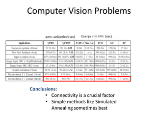
  • 8. Computer Vision Problems perc. unlabeled (sec) Energy (sec) Conclusions: • Connectivity is a crucial factor • Simple methods like Simulated Annealing sometimes best
  • 9. Diagram Recognition [Szummer et al ‘04] 71 nodes; 4.8 con.; 28% non-sub; 0.5 unary strength • 2700 test cases: QPBO solved nearly all (QPBOP solves all) Ground truth QPBOP (0sec) - Global Min. Sim. Ann. E=0 (0.28sec) QPBO: 56.3% unlabeled (0 sec) BP E=25 (0 sec) GrapCut E= 119 (0 sec) ICM E=999 (0 sec)
  • 10. Binary Image Deconvolution 50x20 nodes; 80con; 100% non-sub; 109 unary strength Ground Truth Input 0.2 0.2 0.2 0.2 0.2 0.2 0.2 0.2 0.2 0.2 0.2 0.2 0.2 0.2 0.2 0.2 0.2 0.2 0.2 0.2 0.2 0.2 0.2 0.2 0.2 5x5 blur kernel MRF: 80 connectivity - illustration
  • 11. Binary Image Deconvolution 50x20 nodes; 80con; 100% non-sub; 109 unary strength Ground Truth Input QPBO 80% unlab. (0.1sec) QPBOP 80% unlab. (0.9sec) ICM E=6 (0.03sec) GC E=999 (0sec) BP E=71 (0.9sec) QPBOP+BP+I, E=8.1 (31sec) Sim. Ann. E=0 (1.3sec)
  • 12. Comparison papers • Binary, highly-connected MRFs *Rother et al. ‘07+ Conclusion: low-connectivity tractable: QPBO(P) • Multi-label, 4-connected MRFs *Szeliski et al ‘06,‘08+ all online: http://vision.middlebury.edu/MRF/ • Multi-label, highly-connected MRFs *Kolmogorov et al ‘06+
  • 13. Comparison papers • Binary, highly-connected MRFs *Rother et al. ‘07+ Conclusion: low-connectivity tractable: QPBO(P) • Multi-label, 4-connected MRFs *Szeliski et al ‘06,‘08+ all online: http://vision.middlebury.edu/MRF/ • Multi-label, highly-connected MRFs *Kolmogorov et al ‘06+
  • 14. Multiple labels – 4 connected “Attractive Potentials” stereo Panoramic stitching Image Segmentation; de-noising; in-painting [Szelsiki et al ’06,08+
  • 15. Stereo image Ground TRW-S image Ground TRW-S truth truth Conclusions: – Solved by alpha-exp. and TRW-S (within 0.01%-0.9% of lower bound – true for all tests!) – Expansion-move always better than swap-move
  • 16. De-noising and in-painting Ground truth Noisy input TRW-S Alpha-exp. Conclusion: – Alpha-expansion has problems with smooth areas (potential solution: fusion-move *Lempitsky et al. ‘07+)
  • 17. Panoramic stitching • Unordered labels are (slightly) more challenging
  • 18. Comparison papers • Binary, highly-connected MRFs *Rother et al. ‘07+ Conclusion: low-connectivity tractable (QPBO) • Multi-label, 4-connected MRFs *Szeliski et al ‘06,‘08+ all online: http://vision.middlebury.edu/MRF/ Conclusion: solved by expansion-move; TRW-S (within 0.01 - 0.9% of lower bound) • Multi-label, highly-connected MRFs *Kolmogorov et al ‘06+
  • 19. Comparison papers • Binary, highly-connected MRFs *Rother et al. ‘07+ Conclusion: low-connectivity tractable (QPBO) • Multi-label, 4-connected MRFs *Szeliski et al ‘06,‘08+ all online: http://vision.middlebury.edu/MRF/ Conclusion: solved by expansion-move; TRW-S (within 0.01 - 0.9% of lower bound) • Multi-label, highly-connected MRFs *Kolmogorov et al ‘06+
  • 20. Multiple labels – highly connected Stereo with occlusion: E(d): {1,…,D}2n → R Each pixel is connected to D pixels in the other image *Kolmogorov et al. ‘06+
  • 21. Multiple labels – highly connected Tsukuba: 16 labels Cones: 56 labels • Alpha-exp. considerably better than message passing Potential reason: smaller connectivity in one expansion-move
  • 22. Comparison: 4-con. versus highly con. Tsukuba (E) Map (E) Venus (E) highly-con. 103.09% 103.28% 102.26% 4-con. 100.004% 100.056% 100.014% Lower-bound scaled to 100% Conclusion: • highly connected graphs are harder to optimize
  • 23. Comparison papers • binary, highly-connected MRFs *Rother et al. ‘07+ Conclusion: low-connectivity tractable (QPBO) • Multi-label, 4-connected MRFs *Szeliski et al ‘06,‘08+ all online: http://vision.middlebury.edu/MRF/ Conclusion: solved by alpha-exp.; TRW (within 0.9% to lower bound) • Multi-label, highly-connected MRFs *Kolmogorov et al ‘06+ Conclusion: challenging optimization (alpha-exp. best) How to efficiently optimize general highly-connected (higher-order) MRFs is still an open question
  • 24. Course Program 9.30-10.00 Introduction (Andrew Blake) 10.00-11.00 Discrete Models in Computer Vision (Carsten Rother) 15min Coffee break 11.15-12.30 Message Passing: DP, TRW, LP relaxation (Pawan Kumar) 12.30-13.00 Quadratic pseudo-boolean optimization (Pushmeet Kohli) 1 hour Lunch break 14:00-15.00 Transformation and move-making methods (Pushmeet Kohli) 15:00-15.30 Speed and Efficiency (Pushmeet Kohli) 15min Coffee break 15:45-16.15 Comparison of Methods (Carsten Rother) 16:15-17.30 Recent Advances: Dual-decomposition, higher-order, etc. (Carsten Rother + Pawan Kumar) All online material will be online (after conference): http://research.microsoft.com/en-us/um/cambridge/projects/tutorial/
  • 25. Advanced Topics – Optimizing Higher-Order MRFs Carsten Rother Microsoft Research Cambridge
  • 26. Challenging Optimization Problems • How to solve higher-order MRFs: • Possible Approaches: - Convert to Pairwise MRF (Pushmeet has explained) - Branch & MinCut (Pushmeet has explained) - Add global constraint to LP relaxation - Dual Decomposition
  • 27. Add global constraints to LP Basic idea: T ∑ Xi ≥ 1 i Є T References: [K. Kolev et al. ECCV’ 08] silhouette constraint [Nowizin et al. CVPR ‘09+ connectivity prior [Lempitsky et al ICCV ‘09+ bounding box prior (see talk on Thursday) See talk on Thursday: [Lempitsky et al ICCV ‘09+ bounding box prior
  • 28. Dual Decomposition • Well known in optimization community [Bertsekas ’95, ‘99+ • Other names: “Master-Slave” [Komodiakis et al. ‘07, ’09+ • Examples of Dual-Decomposition approaches: – Solve LP of TRW [Komodiakis et al. ICCV ‘07+ – Image segmentation with connectivity prior [Vicente et al CVPR ‘08+ – Feature Matching [Toressani et al ECCV ‘08+ – Optimizing Higher-Order Clique MRFs [Komodiakis et al CVPR ‘09+ – Marginal Probability Field *Woodford et al ICCV ‘09+ – Jointly optimizing appearance and Segmentation [Vicente et al ICCV 09]
  • 29. Dual Decomposition Hard to optimize Possible to optimize Possible to optimize min E(x) = min [ E1(x) + θTx + E2(x) – θTx ] x x ≥ min [E1(x1) + θTx1] + min [E2(x2) - θTx2] = L(θ) x1 x2 “Lower bound” • θ is called the dual vector (same size as x) • Goal: max L(θ) ≤ min E(x) θ x • Properties: • L(θ) is concave (optimal bound can be found) • If x1=x2 then problem solved (not guaranteed)
  • 30. Why is the lower bound a concave function? L(θ) = min [E1(x1) + θTx1] + min [E2(x2) - θTx2] L(θ) : Rn -> R x1 x2 L1(θ) L2(θ) θTx’1 L1(θ) θTx’’1 θTx’’’1 θ L(θ) concave since a sum of concave functions
  • 31. How to maximize the lower bound? If L(θ) were to be differentiable use gradient ascent L(θ) not diff. … so subgradient approach [Shor ‘85+
  • 32. How to maximize the lower bound? If L(θ) were to be differentiable use gradient ascent L(θ) not diff. so subgradient approach [Shor ‘85+ L(θ) = min [E1(x1) + θTx1] + min [E2(x2) - θTx2] L(θ) : Rn -> R x1 x2 L1(θ) L2(θ) θTx’1 L1(θ) θTx’’1 Subgradient g θTx’’’1 Θ’ Θ’’ Θ Θ’’ = Θ’ + λ g = Θ’ + λ x’1 Θ’’ = Θ’ + λ (x1-x2)
  • 33. Dual Decomposition L(θ) = min [E1(x1) + θTx1] + min [E2(x2) - θTx2] x1 x2 Subgradient Optimization: “Master” Θ = Θ + λ(x*-x2) 1 * x1* x2 * Θ Θ subgradient Subproblem 1 Subproblem 2 x* = min [E1(x1) + θTx1] 1 x2 = min [E2(x2) + θTx2] * “Slaves” x1 x2 • Guaranteed to converge to optimal bound L(θ) • Choose step-width λ correctly ([Bertsekas ’95]) • Pick solution x as the best of x1 or x2 • E and L can in- and decrease during optimization • Each step: θ gets close to optimal θ* Example optimization
  • 34. Why can the lower bound go down? Lower envelop of planes in 3D: L(θ) L(θ’) L(θ’) ≤ L(θ)
  • 35. Analyse the model push x1p towards 0 1 push x2p towards 1 0 L(θ) = min [E1(x1) + θTx1] + min [E2(x2) - θTx2] Update step: Θ’’ = Θ’ + λ (x*-x*) 1 2 Look at pixel p: Case1: x* = x2p 1p * then Θ’’ = Θ’ Case2: x* = 1 x2p = 0 1p * then Θ’’ = Θ’+ λ Case3: x* = 0 x* = 1 1p 2p then Θ’’ = Θ’- λ
  • 36. Example 1: Segmentation and Connectivity Foreground object must be connected: E(x) = ∑ θi (xi) + ∑ θij (xi,xj) + h(x) h(x)= { ∞ if x not 4-connected 0 otherwise Zoom in User input Standard MRF Standard MRF +h *Vicente et al ’08+
  • 37. Example 1: Segmentation and Connectivity E1(x) E(x) = ∑ θi (xi) + ∑ θij (xi,xj) + h(x) h(x)= { ∞ if x not 4-connected 0 otherwise Derive Lower bound: min E(x) = min [ E1(x) + θTx + h(x) – θTx ] x x ≥ min [E1(x1) + θTx1] + min [h(x2) + θTx2] = L(θ) x1 x2 Subproblem 1: Subproblem 2: Unary terms + Unary terms + pairwise terms Connectivity constraint Global minimum: Global minimum: GraphCut Dijkstra But: Lower bound was for no example tight.
  • 38. Example 1: Segmentation and Connectivity E1(x) E(x) = ∑ θi (xi) + ∑ θij (xi,xj) + h(x) h(x)= { ∞ if x not 4-connected 0 otherwise Derive Lower bound: x’ indicator vector of all pairwise terms min E(x) = min [ E1(x) + θTx + θ’Tx’ + h(x) – θTx + h(x) - θ’Tx’] x,x’ x,x’ ≥ min [E1(x1) + θTx1 + θ’Tx’1] + min [h(x2) + θTx2] + x1,x’1 x2 min [h(x3) + θ’Tx’3] =L(θ) x3,x’3 Subproblem 1: Subproblem 2: Subproblem 3: Unary terms + Unary terms + Pairwise terms + pairwise terms Connectivity constraint Connectivity constraint Global minimum: Global minimum: Lower Bound: Based on GraphCut Dijkstra minimal paths on a dual graph
  • 39. Results: Segmentation and Connectivity Global optimum 12 out of 40 cases. Extra Input GlobalMin Image Input GraphCut Heuristic method, DijkstraGC, which is faster and gives empirically same or better results *Vicente et al ’08+
  • 40. Example2: Dual of the LP Relaxation (from Pawan Kumar’s part) q*( i) = min iTx i xi Wainwright et al., 2001 1 q*( 1) Va Vb Vc Va Vb Vc 2 q*( 2) Vd Ve Vf Vd Ve Vf 3 q*( 3) V V g V h i Vg Vh Vi q*( 4) q*( 5) q*( 6) =( a0, a1,…, ab00, ab01,…) Va Vb Vc i≥ 0 x = (xa0, xa1,…,xab00,xab01,…) Vd Ve Vf Dual of LP Vg Vh Vi max i q*( i) = L({ i}) { i} i 4 5 6 i i = i
  • 41. Example2: Dual of the LP Relaxation “Original “i different “Lower bound” problem” trees” min Tx = min iTx x ∑ ≥ ∑ min x iTx i = L({ i}) x i i i q*( i) Subject to i = i Use subgradient … why? θTx’1 q*( i) concave wrt i ; q*( i) = min iTx i θTx’’1 xi θTx’’’1 Projected subgradient method: θ Θi = [Θi + λx *] i Ω Ω= {Θi| ∑ Θi = Θ } i Guaranteed to get the optimal lower bound !
  • 42. Example 2: optimize LP of TRW TRW-S: • Not guaranteed to get optimal bound (DD does) • Lower bound goes always up (DD not). • Needs min-marginals (DD not) • DD paralizable (every tree in DD can be optimized separately) [Komodiakis et al ’07+
  • 43. Example 3: A global perspective on low-level vision Global unary, er. 12.8% Cost f 0 n ∑xi Not NP-hard i Add global term which enforces (Pushmeet Kohli’s part) a match with the marginal statistic Cost f E(x) = ∑ θi (xi) + ∑ θij (xi,xj) + f(∑xi) “Solve with dual- i i,jЄN i decomposition” E1 E2 0 n ∑xi *Woodford et al. ICCV’09+ i (see poster on Friday)
  • 44. Example 3: A global perspective on low-level vision Image de-noising Ground truth Noisy input Pairwise-MRF Global gradient Gradient strength prior Image synthesis input [Kwatra ’03+ global color distribution prior
  • 45. Example 4: Solve GrabCut globally optimal w Color model E(x, w) E’(x) = min E(x, w) w Highly connected MRF Higher-order MRF E(x,w): {0,1}n x {GMMs}→ R E(x,w) = ∑ θi (xi,w) + ∑ θij (xi,xj) *Vicente et al; ICCV ’09+ (see poster on Tuesday)
  • 46. Example 4: Solve GrabCut globally optimal E(x)= g(∑xi) + ∑ fb(∑xib) + ∑ θij (xi,xj) “Solve with dual- i b i,jЄN decomposition” E1 E2 g convex fb concave 0 n/2 n ∑xi 0 max ∑xib Prefers “equal area” segmentation Each color either fore- or background input
  • 47. Example 3: Solve GrabCut globally optimal Globally optimal in 60% of cases, such as… *Vicente et al; ICCV ’09+ (see poster on Tuesday)
  • 48. Summary • Dual Decomposition is a powerful technique for challenging MRFs • Not guaranteed to give globally optimal energy • … but for several vision problems we get tight bounds
  • 49. END
  • 51. Texture Restoration (table 1) 256x85 nodes; 15connec; 36% non-sub; 6.6 unary strength Training Image Test Image GC, E=999 QPBO, QPBOP, (0.05sec) 16.5% unlab. 0% unlab. (14sec) (1.4sec) Global Minimum. Sim. ann., ICM, BP, BP+I, C+BP+I (visually similar)
  • 52. New-View Synthesis [Fitzgibbon et al ‘03] 385x385 nodes; 8con; 8% non-sub; 0.1 unary strength Ground Truth Graph Cut E=2 (0.3sec) Sim. Ann. E=980 (50sec) ICM E=999 (0.2sec) (visually similar) QPBO 3.9% unlabelled QPBOP - Global Min. (1.4sec), BP E=18 (0.6sec) (black) (0.7sec) P+BP+I, BP+I
  • 53. Image Segmentation – region & boundary brush 321x221 nodes; 4con; 0.006% non-sub; 0 unary strength Input Image User Input Sim. Ann. E=983 (50sec) ICM E=999 (0.07sec) GraphCut E=873 (0.11sec) BP E=28 (0.2sec) QPBO 26.7% unlabeled QPBOP Global Min (3.8sec) (0.08sec)
  • 54. Non-truncated cost function [HBF; Szeliski ‘06+ Fast linear system solver in continuous domain (then discretised) cost |di-dj| original input HBF