SlideShare a Scribd company logo
Algorithm Analysis & Data Structures Jaideep Srivastava
Schedule of topics Lecture 1: Algorithm analysis Concept – what is it? Importance – why do it? Examples – lots of it Formalism Lecture 2: Recursion Concept Examples Lecture 3: Trees Concept & properties Tree algorithms
Introduction A famous quote: Program = Algorithm + Data Structure. All of you have programmed; thus have already been exposed to algorithms and data structure.  Perhaps you didn't see them as separate entities; Perhaps you saw data structures as simple programming constructs (provided by STL--standard template library). However, data structures are quite distinct from algorithms, and very important in their own right.
Lecture 1 – Algorithm Analysis & Complexity
Objectives The main focus of is to introduce you to a systematic study of algorithms and data structures.  The two guiding principles of the course are: abstraction and formal analysis. Abstraction: We focus on topics that are broadly applicable to a variety of problems. Analysis: We want a formal way to compare two objects (data structures or algorithms). In particular, we will worry about "always correct"-ness, and worst-case bounds on time and memory (space).
What is Algorithm Analysis For Foundations of Algorithm Analysis and Data Structures.  Analysis: How to predict an algorithm’s performance  How well an algorithm scales up How to compare different algorithms for a problem Data Structures How to efficiently store, access, manage data  Data structures effect algorithm’s performance
Example Algorithms Two algorithms for computing the Factorial  Which one is better? int factorial (int n) { if (n <= 1)  return 1; else  return n * factorial(n-1); } int factorial (int n) { if (n<=1)  return 1; else { fact = 1; for (k=2; k<=n; k++)  fact *= k; return fact; } }
Examples of famous algorithms Constructions of Euclid Newton's root finding  Fast Fourier Transform ( signal processing ) Compression (Huffman, Lempel-Ziv, GIF, MPEG) DES, RSA encryption ( network security ) Simplex algorithm for linear programming ( optimization ) Shortest Path Algorithms (Dijkstra, Bellman-Ford) Error correcting codes (CDs, DVDs) TCP congestion control, IP routing ( computer networks ) Pattern matching ( Genomics )  Search Engines ( www )
Role of Algorithms in Modern World Enormous amount of data  Network traffic (telecom billing, monitoring) Database transactions (Sales, inventory) Scientific measurements (astrophysics, geology) Sensor networks. RFID tags Radio frequency identification  ( RFID ) is a method of remotely storing and retrieving data using devices called  RFID tags.   Bioinformatics (genome, protein bank)
A real-world Problem Communication in the Internet Message (email, ftp) broken down into IP packets. Sender/receiver identified by IP address. The packets are routed through the Internet by special computers called Routers. Each packet is stamped with its destination address, but not the route. Because the Internet topology and network load is constantly changing, routers must discover routes dynamically. What should the Routing Table look like?
IP Prefixes and Routing Each router is really a switch: it receives packets at several input ports, and appropriately sends them out to output ports. Thus, for each packet, the router needs to transfer the packet to that output port that  gets it closer to its destination . Should each router keep a table: IP address x Output Port? How big is this table? When a link or router fails, how much information would need to be modified? A router typically forwards several million packets/sec!
Data Structures The IP packet forwarding is a Data Structure problem! Efficiency, scalability  is very important. Similarly, how does Google find the documents matching your query so fast? Uses sophisticated algorithms to create index structures, which are just data structures. Algorithms and data structures are ubiquitous. With the data glut created by the new technologies, the need to organize, search, and update  MASSIVE  amounts of information  FAST  is more severe than ever before.
Algorithms to Process these Data Which are the top K sellers? Correlation between time spent at a web site and purchase amount? Which flows at a router account for > 1% traffic? Did source S send a packet in last s seconds? Send an alarm if any international arrival matches a profile in the database Similarity matches against genome databases Etc.
Max Subsequence Problem Given a sequence of integers A1, A2, …, An, find the maximum possible value of a  subsequence  Ai, …, Aj. Numbers can be negative. You want a  contiguous  chunk with largest sum. Example:  -2, 11, -4, 13, -5, -2 The answer is  20  (subseq.  A2 through A4). We will discuss  4 different algorithms , with time complexities  O(n 3 ), O(n 2 ), O(n log n), and O(n). With n = 10 6 , algorithm 1 may take > 10 years;  algorithm 4 will take a fraction of a second!
Algorithm 1 for Max Subsequence Sum Given  A 1 ,…,A n  ,  find the maximum value of  A i +A i+ 1 + ··· +A j 0 if the max value is negative  int maxSum = 0; for( int i = 0; i < a.size( ); i++ ) for( int j = i; j < a.size( ); j++ ) { int thisSum = 0; for( int k = i; k <= j; k++ ) thisSum += a[ k ]; if( thisSum > maxSum ) maxSum  = thisSum; } return maxSum; Time complexity:  O  n 3 
Algorithm 2 Idea: Given sum from i to j-1, we can compute the sum from i to j in constant time.  This eliminates one nested loop, and reduces the running time to O(n 2 ). into maxSum = 0; for( int i = 0; i < a.size( ); i++ ) int thisSum = 0; for( int j = i; j < a.size( ); j++ ) {   thisSum += a[ j ];   if( thisSum > maxSum )   maxSum  = thisSum; } return maxSum;
Algorithm 3 This algorithm uses divide-and-conquer paradigm. Suppose we split the input sequence at midpoint. The max subsequence is entirely in the  left half , entirely in the  right half , or it  straddles the midpoint . Example: left half  | right half 4  -3  5 -2 |  -1  2  6  -2 Max in left is  6  (A1 through A3); max in right is  8  (A6 through A7).  But straddling max is 11 (A1 thru A7).
Algorithm 3 (cont.) Example: left half  | right half 4  -3  5  -2  |  -1  2  6  -2 Max subsequences in each half found by recursion. How do we find the straddling max subsequence? Key Observation :  Left half of the straddling sequence is the max subsequence ending with -2. Right half is the max subsequence beginning with -1. A linear scan lets us compute these in O(n) time.
Algorithm 3:  Analysis The divide and conquer is best analyzed through recurrence: T(1) = 1 T(n) = 2T(n/2) + O(n) This recurrence solves to T(n) = O(n log n).
Algorithm 4 Time complexity clearly  O ( n ) But why does it work? I.e. proof of correctness. 2, 3, -2, 1, -5, 4, 1, -3, 4, -1, 2 int maxSum = 0, thisSum = 0; for( int j = 0; j < a.size( ); j++ ) { thisSum += a[ j ]; if ( thisSum > maxSum ) maxSum = thisSum; else if ( thisSum < 0 ) thisSum = 0; } return maxSum; }
Proof of Correctness Max subsequence cannot  start or end  at a negative Ai. More generally, the max subsequence cannot have a prefix with a negative sum. Ex:  -2  11  -4  13  -5  -2 Thus, if we ever find that Ai through Aj sums to < 0, then we can advance i to j+1 Proof. Suppose j is the first index after i when the sum becomes < 0 The max subsequence cannot start at any p between i and j. Because A i  through A p-1  is positive, so starting at i would have been even better.
Algorithm 4 int maxSum = 0, thisSum = 0; for( int j = 0; j < a.size( ); j++ ) { thisSum += a[ j ]; if ( thisSum > maxSum ) maxSum = thisSum; else if ( thisSum < 0 ) thisSum = 0; } return maxSum The algorithm resets whenever prefix is < 0. Otherwise, it forms new sums and updates maxSum in one pass.
Why Efficient Algorithms Matter Suppose N = 10 6 A PC can read/process N records in 1 sec. But if some algorithm does N*N computation, then it  takes 1M seconds = 11 days!!! 100 City  Traveling Salesman Problem .  A supercomputer checking 100 billion tours/sec still requires 10 100   years! Fast  factoring  algorithms can break encryption schemes. Algorithms research determines what is safe code length. (> 100 digits)
How to Measure Algorithm Performance What metric should be used to judge algorithms? Length of the program (lines of code) Ease of programming (bugs, maintenance) Memory required Running time Running time is the dominant standard. Quantifiable and easy to compare Often the critical bottleneck
Abstraction An algorithm may run differently depending on: the hardware platform (PC, Cray, Sun) the programming language (C, Java, C++) the programmer (you, me, Bill Joy) While different in detail, all hardware and programming models are equivalent in some sense:  Turing machines .  It suffices to count basic operations. Crude but valuable measure of algorithm’s performance  as a function of input size .
Average, Best, and Worst-Case On which input instances should the algorithm’s performance be judged? Average case: Real world distributions difficult to predict Best case: Seems unrealistic Worst case: Gives an absolute guarantee We will use the worst-case measure.
Examples Vector addition  Z =  A+B for (int i=0; i<n; i++) Z[i] = A[i] + B[i]; T(n) = c n Vector (inner) multiplication  z =A*B z = 0; for (int i=0; i<n; i++) z = z + A[i]*B[i]; T(n) = c’ + c 1  n
Examples Vector (outer) multiplication  Z = A*B T for (int i=0; i<n; i++) for (int j=0; j<n; j++) Z[i,j] = A[i] * B[j]; T(n) = c 2  n 2 ; A program does all the above T(n) = c 0  + c 1  n + c 2  n 2 ;
Simplifying the Bound T(n) = c k  n k  + c k-1  n k-1  + c k-2  n k-2  + … + c 1   n + c o too complicated too many terms Difficult to compare two expressions, each with 10 or 20 terms  Do we really need that many terms?
Simplifications Keep just one term!  the fastest growing term (dominates the runtime) No constant coefficients are kept Constant coefficients affected by machines, languages, etc. Asymtotic behavior  (as  n  gets large) is determined entirely by the  leading  term. Example . T(n) = 10 n 3  + n 2  + 40n + 800 If n = 1,000, then  T(n) = 10,001,040,800 error is 0.01% if we drop all but the  n 3   term In an assembly line the slowest worker determines the throughput rate
Simplification Drop the constant coefficient Does not effect the relative order
Simplification The  faster  growing term (such as 2 n )  eventually  will outgrow the slower growing terms (e.g., 1000 n) no matter what their coefficients! Put another way, given a certain increase in allocated time, a higher order algorithm will not reap the benefit by solving much larger problem
Complexity and Tractability  Assume the computer does 1 billion ops per sec.
2 n n 2 n  log  n n log  n log  n n n  log  n n 2 n 3 n 3 2 n
Another View More resources (time and/or processing power) translate into large problems solved if complexity is low 1.3 13 10 2 n 2.2 22 10 N 3 3.2 45 14 5n 2 10 10 1 1000n 10 100 10 100n Increase in Problem size Problem size solved in 10 4  sec Problem size solved in 10 3  sec T(n)
Asymptotics They all have the same “growth” rate
Caveats Follow the spirit, not the letter a 100n algorithm is more expensive than n 2  algorithm when n < 100 Other considerations: a program used only a few times  a program run on small data sets ease of coding, porting, maintenance  memory requirements
Asymptotic Notations Big-O,  “bounded above by”:   T(n) = O(f(n)) For some c and N, T(n)     c·f(n) whenever n > N. Big-Omega,  “bounded below by”:   T(n) =   (f(n)) For some c>0 and N, T(n)     c·f(n) whenever n > N. Same as f(n) = O(T(n)). Big-Theta,  “bounded above and below”:  T(n) =   (f(n)) T(n) = O(f(n))  and also T(n) =   (f(n)) Little-o,  “strictly bounded above”:  T(n) = o(f(n)) T(n)/f(n)    0  as  n     
By Pictures Big-Oh  (most commonly used) bounded above  Big-Omega   bounded below Big-Theta exactly  Small-o not as expensive as ...
Example
Examples
Summary (Why O(n)?) T(n) = c k  n k  + c k-1  n k-1  + c k-2  n k-2  + … + c 1   n + c o Too complicated O(n k  ) a single term with constant coefficient dropped Much simpler, extra terms and coefficients  do not matter  asymptotically Other criteria hard to quantify
Runtime Analysis Useful rules simple statements (read, write, assign) O(1)  (constant) simple operations (+ -  * / == > >= < <=  O(1) sequence of simple statements/operations rule of sums for, do, while loops rules of products
Runtime Analysis (cont.) Two important rules Rule of sums  if you do a number of operations in sequence, the runtime is dominated by the most expensive operation  Rule of products if you repeat an operation a number of times, the total runtime is the runtime of the operation multiplied by the iteration count
Runtime Analysis (cont.) if (cond) then  O(1) body 1   T 1 (n) else body 2   T 2 (n) endif T(n) = O(max (T 1 (n), T 2 (n))
Runtime Analysis (cont.) Method calls A calls B B calls C etc. A sequence of operations when call sequences are flattened T(n) = max(T A (n), T B (n), T C (n))
Example for (i=1; i<n; i++) if A(i) > maxVal then maxVal= A(i); maxPos= i; Asymptotic Complexity: O(n)
Example for (i=1; i<n-1; i++) for (j=n; j>= i+1;  j--) if (A(j-1) > A(j)) then temp = A(j-1); A(j-1) = A(j); A(j) = tmp; endif endfor endfor Asymptotic Complexity is O(n 2 )
Run Time for Recursive Programs T(n) is defined recursively in terms of T(k), k<n The  recurrence relations  allow T(n) to be “unwound” recursively into some base cases (e.g., T(0) or T(1)).  Examples: Factorial Hanoi towers
Example: Factorial  int factorial (int n) { if (n<=1)  return 1; else  return n * factorial(n-1); } factorial (n) = n*n-1*n-2* … *1 n  * factorial(n-1) n-1  * factorial(n-2) n-2  * factorial(n-3) … 2  *factorial(1)  T(n) T(n-1) T(n-2) T(1)
Example: Factorial (cont.) int factorial1(int n) { if (n<=1)  return 1; else { fact = 1; for (k=2;k<=n;k++)  fact *= k; return fact; } } Both algorithms are O(n).
Example: Hanoi Towers Hanoi(n,A,B,C) =  Hanoi(n-1,A,C,B)+Hanoi(1,A,B,C)+Hanoi(n-1,C,B,A)
// Early-terminating version of selection sort bool sorted = false; !sorted && sorted = true; else sorted = false;   // out of order Worst Case Best Case template<class T> void SelectionSort(T a[], int n) { for (int size=n;  (size>1); size--) { int pos = 0; // find largest for (int i = 1; i < size; i++) if (a[pos] <= a[i]) pos = i; Swap(a[pos], a[size - 1]); } } Worst Case, Best Case, and Average Case
T(N)=6N+4 : n0=4 and c=7, f(N)=N T(N)=6N+4 <= c f(N) = 7N for N>=4 7N+4 = O(N) 15N+20 = O(N) N 2 =O(N)? N log N = O(N)? N log N = O(N 2 )? T(N) f(N) c f(N) n 0 T(N)=O(f(N)) N 2  = O(N log N)? N 10  = O(2 N )? 6N + 4 = W(N) ? 7N?  N+4 ? N 2 ? N log N? N log N = W(N 2 )? 3 = O(1) 1000000=O(1) Sum i = O(N)?
An Analogy: Cooking Recipes Algorithms are detailed and precise instructions. Example: bake a chocolate mousse cake. Convert raw ingredients into processed output. Hardware (PC, supercomputer vs. oven, stove) Pots, pans, pantry are data structures. Interplay of hardware and algorithms  Different recipes for oven, stove, microwave etc.  New advances. New models: clusters, Internet, workstations Microwave cooking, 5-minute recipes, refrigeration
Lecture 2 - Recursion
What is Recursion? Recursion is when a function either directly or indirectly makes a call to itself. Recursion is a powerful problem solving tool. Many mathematical functions and algorithms are most easily expressed using recursion.
How does it work? Functions are implemented using an internal stack of  activation records .  Each time a function is called a new activation record is pushed on the stack. When a function returns, the stack is popped and the activation record of the calling method is on top of the stack.
How does it work? (cont.) The function being called, and whose   activation record is being pushed on the stack, can be different from the calling function (e.g., when main calls a function). The function being called can be a different instance of the calling subprogram.  Each instance of the function has its own parameters and local variables.
Example Many mathematical functions are defined recursively. For example, the factorial function: N! = N * (N-1)!  for N>0 0!  = 1 We have defined factorial in terms of a smaller (or simpler) instance of itself. We must also define a  base   case  or  stopping condition.
Recursive Function Call A  recursive call  is a function call in which the called function is the same as the one making the call. We must avoid making an infinite sequence of function calls (infinite recursion).
Finding a Recursive Solution Each successive recursive call should bring you closer to a situation in which the answer is known.  general (recursive) case A case for which the answer is known (and can be expressed without recursion) is called a  base case .
General format for many recursive functions if  (some conditions for which answer is known)    // base case   solution statement else // general case   recursive function call
Tail Recursion Use only one recursive call at the end of a function void tail (int i) { if (i > 0) { System.out.print( i+ “ ”); tail(i – 1); } } void iterativetail(int i) { for (  ; i > 0; i--) System.out.print( i+ “ ”);   }
NonTail Recursion void nonTail (int i) { if (i > 0) {   nonTail(i – 1); System.out.print( i+ “ ”); nonTail(i – 1); } }
Indirect recursion Receive( buffer ) while buffer is not filled up If information is still incoming get a char and store it in buffer; else exit(); decode(buffer); Decode(buffer) decode information in buffer; store(buffer); Store(buffer) transfer information from buffer to file; receive(buffer);
Nested recursion h(n) { 0  if n=0 h(n) ={  n  if n>4 h(n) { h(2+h(2n)) if n <=4
Writing a recursive function to find  n factorial DISCUSSION  The function call Factorial(4) should have value 24, because that is 4 * 3 * 2 * 1 . For a situation in which the answer is known, the value of 0! is 1. So our  base case  could be along the lines of if  ( number == 0 ) return 1;
Writing a recursive function to find  Factorial(n) Now for the  general case . . . The value of  Factorial(n)  can be written as n  *  the product of the numbers from (n - 1) to 1, that is,    n  *  (n - 1)  *  .  .  .  *  1 or,  n  *  Factorial(n - 1) And notice that the recursive call  Factorial(n - 1) gets us “closer” to the base case of  Factorial(0).
Recursive Function Example: Factorial Problem: calculate n!  (n factorial) n! = 1  if n = 0 n! = 1 * 2 * 3 *...* n  if n > 0 Recursively: if  n = 0 ,  then n! =  1 if n > 0,  then n!  = n * ( n-1 ) !
Factorial Function int RecFactorial( /* in */ int n) // Calculates n factorial, n!  // Precondition: n is a non-negative //  integer {  if ( n <= 0 ) then return  1 else return  n *  RecFa ctorial ( n-1 ) }
1 int fact(int n) 2 { 3  if ( n <= 0 ) then 4   return 1; 5  else 6   return n*fact(n-1); 7 } main(...) {  ...  20   System.out.print(  (fact(3)); ... returns  6   to  main()
Exponentiation base exponent e.g.  5 3 Could be written as a function Power(base, exp)
Can we write it recursively? b e  = b * b (e-1) What’s the limiting case? When e = 0 we have b 0  which always equals? 1
Another Recursive Function 1 function Power returnsa Num(base, exp) 2 // Computes the value of Base Exp   3 // Pre: exp is a non-negative integer  4  if ( exp = 0 ) then 5  returns  1 6  else 7   returns  base *  Power (base,  exp-1 ) 8  endif 9 endfunction  Power  x N  = x * x N -1   for  N >0  x 0  = 1 main(...) {  ...  20  cout << (Power(2,3)); ...
A man has an infant male-female pair of rabbits in a hutch entirely surrounded by a wall. We wish to know how many rabbits can be bred from this pair in one year, if the nature of the rabbits is such that every month they breed one other male-female pair which begins to breed in the second month after their birth. Assume that no rabbits die during the year. The Puzzle
A Tree Diagram for Fibonacci’s Puzzle
Observations The number of rabbits at the beginning of any month equals the number of rabbits of the previous month plus  the number of new pairs . The number of new pairs at the beginning of a month equals the  number of pairs two months ago . One gets the sequence:  1, 1, 2, 3, 5, 8, 13, 21, 34, 55, 89, … 233
Fibonacci sequence Recursive definition f(1) = 1 f(2) = 1 f(n) = f(n-1) + f(n-2)
Fibonacci Number Sequence if n = 1, then  Fib(n) =   1 if n = 2, then  Fib(n) =  1 if n > 2, then  Fib(n) =  Fib(n-2) + Fib(n-1)   Numbers in the series: 1,  1,  2,  3,  5,  8,  13,  21,  34, ... A More Complex Recursive Function
Fibonacci Sequence Function function Fib returnsaNum (n) // Calculates the nth Fibonacci number  // Precondition: N is a positive integer  if ( (n = 1)  OR (n = 2) ) then returns  1 else returns   Fib ( n-2 ) +  Fib ( n-1 ) endif endfunction //Fibonacci
Tracing with Multiple Recursive Calls Main Algorithm:  answer <- Fib(5)
Tracing with Multiple Recursive Calls Main Algorithm:  answer <- Fib(5) Fib(5):  Fib returns  Fib(3)  + Fib(4)
Tracing with Multiple Recursive Calls Main Algorithm:  answer <- Fib(5) Fib(5):  Fib returns  Fib(3)  + Fib(4) Fib(3):  Fib returns  Fib(1)  + Fib(2)
Tracing with Multiple Recursive Calls Main Algorithm:  answer <- Fib(5) Fib(5):  Fib returns  Fib(3)  + Fib(4) Fib(3):  Fib returns  Fib(1)  + Fib(2) Fib(1):  Fib returns 1
Tracing with Multiple Recursive Calls Main Algorithm:  answer <- Fib(5) Fib(5):  Fib returns  Fib(3)  + Fib(4) Fib(3):  Fib returns 1 +  Fib(2)
Tracing with Multiple Recursive Calls Main Algorithm:  answer <- Fib(5) Fib(5):  Fib returns  Fib(3)  + Fib(4) Fib(3):  Fib returns 1 +  Fib(2) Fib(2):  Fib returns 1
Tracing with Multiple Recursive Calls Main Algorithm:  answer <- Fib(5) Fib(5):  Fib returns  Fib(3)  + Fib(4) Fib(3):  Fib returns 1 + 1
Tracing with Multiple Recursive Calls Main Algorithm:  answer <- Fib(5) Fib(5):  Fib returns 2 +  Fib(4)
Tracing with Multiple Recursive Calls Main Algorithm:  answer <- Fib(5) Fib(5):  Fib returns 2 +  Fib(4) Fib(4):  Fib returns  Fib(2)  + Fib(3)
Tracing with Multiple Recursive Calls Main Algorithm:  answer <- Fib(5) Fib(5):  Fib returns 2 +  Fib(4) Fib(4):  Fib returns  Fib(2)  + Fib(3) Fib(2):  Fib returns 1
Tracing with Multiple Recursive Calls Main Algorithm:  answer <- Fib(5) Fib(5):  Fib returns 2 +  Fib(4) Fib(4):  Fib returns 1 +  Fib(3)
Tracing with Multiple Recursive Calls Main Algorithm:  answer <- Fib(5) Fib(5):  Fib returns 2 +  Fib(4) Fib(4):  Fib returns 1 +  Fib(3) Fib(3):  Fib returns  Fib(1)  + Fib(2)
Tracing with Multiple Recursive Calls Main Algorithm:  answer <- Fib(5) Fib(5):  Fib returns 2 +  Fib(4) Fib(4):  Fib returns 1 +  Fib(3) Fib(3):  Fib returns  Fib(1)  + Fib(2) Fib(1):  Fib returns 1
Tracing with Multiple Recursive Calls Main Algorithm:  answer <- Fib(5) Fib(5):  Fib returns 2 +  Fib(4) Fib(4):  Fib returns 1 +  Fib(3) Fib(3):  Fib returns 1 +  Fib(2)
Tracing with Multiple Recursive Calls Main Algorithm:  answer <- Fib(5) Fib(5):  Fib returns 2 +  Fib(4) Fib(4):  Fib returns 1 +  Fib(3) Fib(3):  Fib returns 1 +  Fib(2) Fib(2):  Fib returns 1
Tracing with Multiple Recursive Calls Main Algorithm:  answer <- Fib(5) Fib(5):  Fib returns 2 +  Fib(4) Fib(4):  Fib returns 1 +  Fib(3) Fib(3):  Fib returns 1 + 1
Tracing with Multiple Recursive Calls Main Algorithm:  answer <- Fib(5) Fib(5):  Fib returns 2 +  Fib(4) Fib(4):  Fib returns 1 + 2
Tracing with Multiple Recursive Calls Main Algorithm:  answer <- Fib(5) Fib(5):  Fib returns 2 + 3
Tracing with Multiple Recursive Calls Main Algorithm:  answer <- 5
Fib(5) 15 calls to Fib to find the 5th Fibonacci number!!! Fib(3) Fib(4) Fib(3) Fib(2) Fib(2) Fib(1) Fib(1) Fib(0) Fib(1) Fib(0) Fib(2) Fib(1) Fib(1) Fib(0)
Excessive Recursion-Fibonacci recursion Int iterativeFib ( int n ) if ( n < 2) return n; else { int i=2, tmp,current = 1, last=0; for ( ; i<=n; ++i) { tmp=current; current+=last; last=tmp; } return current; } }
 
 
Rules of Recursion First two fundamental rules of recursion: Base cases:  Always have at least one case that can be solved without using recursion. Make progress:   Any recursive call must make progress towards the base case.
Rules of Recursion Third fundamental rule of recursion: “ You gotta believe”:  Always assume that the recursive call works.
Rules of Recursion Fourth fundamental rule of recursion: Compound interest rule:  Never duplicate work by solving the same instance of a problem in separate recursive calls.
Towers of Hanoi The puzzle consisted of N disks and three poles: A (the source), B (the destination), and C (the spare)
Towers of Hanoi B C A
Towers of Hanoi A pseudocode description of the solution is: Towers(Count, Source, Dest, Spare) if (Count is 1) Move the disk directly from Source to Dest else { Solve Towers(Count-1, Source, Spare, Dest) Solve Towers(1, Source, Dest, Spare) Solve Towers(Count-1, Spare, Dest, Source) }
Towers of Hanoi void solveTowers( int count, char source, char dest, char spare){ if (count == 1) cout<<“Move disk from pole “ << source  << &quot; to pole &quot; << destination <<endl; else { towers(count-1, source, spare, destination); towers(1, source, destination, spare); towers(count-1, spare, destination, source); }//end if }//end solveTowers
Recall that . . .  Recursion occurs when a function calls itself  (directly or indirectly). Recursion can be used in place of iteration (looping). Some functions can be written more easily using recursion.
Pascal Triangle (Is this recursive?)
Pascal Triangle The combinations of n items taken r at a time . For example: three items:     a    b    c taken 2 at a time:     ab    ac    bc Thus there are three combinations of 3 items taken 2 at a time. In General:     C(n,r) = n!/(r!(n-r)!)     Obviously you can calculate  C(n,r)  using factorials.
Pascal Triangle This leads to Pascal Triangle: n      0                             1              1                        1       1              2                     1     2      1              3                 1     3      3     1              4             1     4      6      4    1              5         1     5      10     10    5    1 This can also be written:              r     0    1    2    3     4    5          n  0     1              1     1     1              2     1     2    1              3     1     3    3    1              4     1     4    6    4    1              5     1     5   10  10    5    1
Pascal Triangle Note from Pascal's Triangle that:      C(n,r) = C(n-1, r-1) + C(n-1,r) This leads to the recurrence for nonnegative r and n, C(n,r) =                1             if r = 0 or r = n,                             0             if r > n,                             C(n-1, r-1) + C(n-1,r)     otherwise.
Pascal Triangle This immediately leads to the recursive function for combinations:   int C(int n, int r) {   if((r == 0) || (r == n))      return 1;   else if(r > n)        return 0;    else         return C(n-1, r-1) + C(n-1, r);     }
What is the value of  rose(25) ? int  rose (int  n) { if  ( n == 1 )  // base case return  0; else  // general case return ( 1 + rose ( n / 2 ) ); }
Finding the value of  rose(25) rose(25)   the original call =  1 +  rose(12)  first recursive call =  1 +  ( 1 + rose(6)   )  second recursive call =  1 + ( 1 + ( 1 + rose(3) ) )  third recursive call =  1 + ( 1 + ( 1 + (1 + rose(1) ) ) )  fourth recursive call =  1 +  1 +  1  +  1 + 0 =  4
Writing recursive functions There must be at least one base case, and at least one general (recursive) case.  The general case should bring you “closer” to the base case.  The parameter(s) in the recursive call cannot all be the same as the formal parameters in the heading.  Otherwise, infinite recursion would occur.  In function  rose( ) , the base case occurred when  (n == 1)  was true.  The general case brought us a step closer to the base case, because in the general case the call was to  rose(n/2) , and the argument  n/2  was closer to 1 (than  n  was).
Three-Question Method of verifying  recursive functions Base-Case Question:  Is there a nonrecursive way  out of the function? Smaller-Caller Question:  Does each recursive function call involve a smaller case of the original problem leading to the base case? General-Case Question:  Assuming each recursive call works correctly, does the whole function work correctly?
Guidelines for writing recursive  functions 1. Get an  exact definition  of the problem to be solved. 2.  Determine the size of the problem to be solved  on this call to the function.  On the initial call, the size of the whole problem is expressed by the actual parameter(s). 3. Identify and  solve the base case(s)  which have non-recursive solutions. 4. Identify and  solve the general case(s)  in terms of smaller (recursive) cases of the same problem.
struct  ListType { int  length ;   // number of elements in the list int  info[ MAX_ITEMS ] ; } ; ListType  list ; struct ListType
Recursive function to determine if value is in list PROTOTYPE  bool  ValueInList( ListType  list ,  int  value ,  int  startIndex )    Already searched    Needs to be searched index  of current element to  examine  74  36  . . .  95 list[0]  [1]  [startIndex] 75  29  47  . . . [length -1]
bool  ValueInList (  ListType  list ,  int  value ,  int  startIndex  ) //  Searches list for value between positions startIndex //  and  list.length-1 { if  ( list.info[startIndex] == value ) // one base case return  true ; else  if  (startIndex == list.length -1 )  // another base case   return  false ;   else   // general case   return ValueInList( list, value, startIndex + 1 ) ; }
“ Why use recursion?” Many solutions could have been written without recursion, by using iteration instead.  The iterative solution uses a loop, and the recursive solution uses an if statement. However, for certain problems the recursive solution is the most natural solution.  This often occurs when  pointer  variables are used.
When to Use Recursion If the problem is recursive in nature therefore it is likely the a recursive algorithm will be preferable and will be less complex If running times of recursive and non-recursive algorithms are hardly perceivable, recursive version is better If both recursive and non-recursive algorithms have the same development complexity, a non-recursive version should be preferred A third alternative in some problems is to use table-driven techniques Sometimes we know that we will not use the only a few values of a particular function If this is the case an implementation using a table would probably suffice and the performance will be better int factorial[8] = {1, 1, 2, 6, 24, 120, 720, 5040};
Use a recursive solution when: The depth of recursive calls is relatively “shallow” compared to the size of the problem. The recursive version does about the same amount of work as the nonrecursive version. The recursive version is shorter and simpler than the nonrecursive solution.  SHALLOW DEPTH  EFFICIENCY  CLARITY
Lecture 3 – Binary Trees
Why Trees? Limitations of  Arrays Linked lists Stacks Queues
Trees: Recursive Definition A tree is a collection of nodes. The collection can be empty, or consist of a  “root”  node  R. There is a “directed edge” from  R  to the root of each subtree. The root of each subtree is a “child” of  R .  R  is the “parent” of each subtree root.
Trees: Recursive Definition (cont.) ROOT OF TREE T T1 T2 T3 T4 T5 SUBTREES
Trees: An Example A B C D E F G H I
Trees: More Definitions Nodes with no children are  leaves : (C,E,F,H,I). Nodes with the same parents are  siblings : (B,C,D,E) and (G,H). A  path  from node  n  to node  m  is the sequence of directed edges from  n  to  m . A  length of a path  is the number of edges in the path
Trees: More Definitions (cont.) The  level/depth of node  n  is the length of the path from the root to  n . The level of the root is 0. The  height/depth of a tree  is equal to the maximum level of a node in the tree. The  height of a node  n  is the length of the longest path from  n  to a leaf. The height of a leaf node is 0. The height of a tree is equal to the height of the root node.
Binary Trees – A Informal Definition A binary tree is a tree in which no node can have more than two children. Each node has 0, 1, or 2 children In this case we can keep direct links to the children: struct TreeNode { Object  element; TreeNode *left_child; TreeNode *right_child; };
Binary Trees – Formal Definition A binary tree is a structure that contains no nodes, or  is comprised of three disjoint sets of nodes: a  root a binary tree called its  left subtree a binary tree called its  right subtree A binary tree that contains no nodes is called  empty
Binary Trees: Recursive Definition ROOT OF TREE T T1 T2 SUBTREES *left_child *right_child
Differences Between A Tree & A Binary Tree No node in a binary tree may have more than 2 children, whereas there is no limit on the number of children of a node in a tree. The subtrees of a binary tree are ordered; those of a tree are not ordered.
Differences Between A Tree & A Binary Tree (cont.) The subtrees of a binary tree are ordered; those of a tree are not ordered Are different when viewed as binary trees Are the same when viewed as trees a b a b
Internal and External Nodes Because in a binary tree all the nodes must have the same number of children we are forced to change the concepts slightly We say that all  internal nodes  have two children External nodes  have no children internal node external node
Recursive definition of a Binary Tree Most of concepts related to binary trees can be explained recursive For instance, A binary tree is: An  external node , or An  internal node  connected to a left binary tree and a right binary tree (called left and right subtrees) In programming terms we can see that our definition for a linked list (singly) can be modified to have two links from each node instead of one.
Property2 :  a unique path exists from the root to every other node  What is a binary tree? (cont.)
Mathematical Properties of Binary Trees Let's us look at some important mathematical properties of binary trees A good understanding of these properties will help the understanding of the performance of algorithms that process trees Some of the properties we'll describe relate also the structural properties of these trees. This is the case because performance characteristics of many algorithms depend on these structural properties and not only the number of nodes.
Minimum Number Of Nodes Minimum number of nodes in a binary tree whose height is  h . At least one node at each level. minimum number of nodes is   h + 1
Maximum Number Of Nodes All possible nodes at first h levels are present Maximum number of nodes = 1 + 2 + 4 + 8 + … + 2 h  =  2 h+1  - 1
Number of Nodes & Height Let  n  be the number of nodes in a binary tree whose height is  h . h + 1 <= n <=  2 h+1  – 1 log 2 (n+1)-1 <= h <= n -1 The  max height  of a tree with  N  nodes is  N - 1  (same as a linked list) The  min height  of a tree with  N  nodes is  log(N+1)-1
Relationship Between Number of Nodes (Internal - External) A binary tree with N internal nodes has N+1 external nodes Let's try to prove this using induction...
Number of edges A binary tree with N internal nodes has 2N edges Let's try to prove this using induction...
Number of edges A binary tree with N nodes (internal and external) has N-1 edges Let's try to prove this using induction...
Binary Tree Representation Array representation Linked representation
Binary Trees Full  binary tree :  All  internal  nodes have two children. Complete  binary tree : All leaves have the same level All  internal nodes  have two children
Node Number Properties  Parent of node  i  is node  i/2 But node  1  is the root and has no parent Left child of node  i   is node  2i But if  2i > n , node   i  has no left child Right child of node  i   is node  2i+1 But if  2i+1 > n , node   i  has no right child Complete  binary tree 1 2 3 4 5 6 7 8 9 10 11 12 13 14 15
Full Binary Tree With n Nodes Start with a complete binary tree that has  at least  n nodes. Number the nodes as described earlier. The binary tree defined by the nodes numbered 1 through n is the unique n node full binary tree. Full binary tree with 11 nodes 1 2 3 4 5 6 7 8 9 10 11 12 13 14 15
Array Representation Number the nodes using the numbering scheme for a full binary tree Store the node numbered i in tree[i] a b c d e f g h i j 1 2 3 4 6 7 8 9 b a c d e f g h i j 1 2 3 4 5 6 7 8 9 10 tree[] 0 5 10
Right-Skewed Binary Tree An n node binary tree needs an array whose length is between n+1 and 2 n If h = n-1 then skewed binary tree a b 1 3 c 7 d 15 tree[] 0 5 10 a - b - - - c - - - - - - - 15 d
Array Representation (cont.) Each tree node is represented as a struct Struct TreeNode { object element; int  child1; int  child2; … int  childn; }; Struct TreeNode tree[100];
Linked Representation Each tree node is represented as an object whose data type is  TreeNode The space required by an n node binary tree is n * (space required by one node)
Trees: Linked representation  Implementation 1 struct TreeNode { Object  element; TreeNode *child1; TreeNode *child2; . . . TreeNode *childn; }; Each node contains a link to all of its children.  This isn’t a good idea, because a node can have an arbitrary number of children!
struct TreeNode { Object  element; TreeNode *child1; TreeNode *sibling; }; Each node contain a link to its first child and a link to its next sibling. This is a better idea. Trees: Linked representation  Implementation 2
Implementation 2: Example / The downward links are to the first child; the horizontal links are to the next sibling. / / / / A / B F / C D E / G H / I /
Binary Trees A  binary tree  is a tree whose nodes have at most two offspring Example struct nodeType { object element; struct nodeType *left, *right; }; struct nodeType *tree;
Linked Representation Example a c b d f e g h leftChild element rightChild root
Some Binary Tree Operations •  Determine the height. •  Determine the number of nodes. •  Make a clone. •  Determine if two binary trees are clones. •  Display the binary tree. •  Evaluate the arithmetic expression represented by a binary tree. •  Obtain the infix form of an expression. •  Obtain the prefix form of an expression. •  Obtain the postfix form of an expression.
CS122 Algorithms and Data Structures Week 7:  Binary Search Trees Binary Expression Trees
Uses for Binary Trees…  --  Binary Search Trees Use for storing and retrieving information Insert, delete, and search faster than with a linked list Idea: Store information in an ordered way (keys)
A Property of Binary Search Trees The key of the root is  larger  than any key in the  left  subtree The key of the root is  smaller  than any key in the  right  subtree Note: Duplicated keys are not allowed
A Property of  Binary Search Tree ROOT OF TREE T T1 T2 SUBTREES *left_child *right_child X All nodes in T1 have keys < X. All nodes in T2 have keys > X.
Binary Search Trees in C++ We will use two classes: The class BinaryNode simply constructs individual nodes in the tree. The class BinarySearchTree maintains a pointer to the root of the binary search tree and includes methods for inserting and removing nodes.
Search Operation BinaryNode *search (const int &x, BinaryNode *t) { if ( t == NULL ) return NULL; if (x == t->key)  return t; // Match if ( x < t->key ) return search( x, t->left ); else  //  t ->key < x return search( x, t->right );  }
FindMin Operation BinaryNode* findMin (BinaryNode *t) { if ( t == NULL ) return NULL; if ( t -> left == NULL ) return t; return findMin (t -> left); } This method returns a pointer to the node containing the smallest element in the tree.
FindMax Operation BinaryNode* findMax (BinaryNode *t) { if ( t == NULL ) return NULL; if ( t -> right == NULL ) return t; return findMax (t -> right); } This function returns a pointer to the node containing the largest element in the tree.
Insert Operation To insert X into a tree T, proceed down the tree as you would with a find. If X is found, do nothing. Otherwise insert X at the last spot on the path that has been traversed.
Insert Operation (cont.) void BinarySearchTree insert (const int &x, BinaryNode *&t) const { if (t == NULL) t = new BinaryNode (x, NULL, NULL); else if (x < t->key) insert(x, t->left); else if( t->key < x) insert(x, t->right); else ;  // Duplicate entry; do nothing } Note the pointer t is passed using call by reference.
Removal Operation If the node to be removed is a leaf, it can be deleted immediately. If the node has  one child , the node can be deleted after its parent adjusts a link to bypass the deleted node.
If the node to be removed  has two children , the general strategy is to replace the data of this node with the  smallest  key of the  right subtree . Then the node with the smallest data is now removed (this case is easy since this node cannot have two children). Removal Operation (cont.)
Removal Operation (cont.) void  remove (const int &x, BinaryNode* &t) const { if ( t == NULL ) return;  // key is not found; do nothing if ( t->key == x) { if( t->left != NULL && t->right != NULL ) {  // Two children t->key = findMin( t->right )->key; remove( t->key, t->right );  } else  {  // One child BinaryNode *oldNode = t; t = ( t->left != NULL ) ? t->left : t->right; delete oldNode;  } }  else {  // Two recursive calls if ( x < t->key )  remove( x, t->left ); else if( t->key < x ) remove( x, t->right ); } }
Deleting by merging
Deleting by merging
Deleting by copying
Balancing a binary tree A binary tree is height-balanced or simply balanced if the difference in height of both the subtrees is either zero or one Perfectly balanced if all leaves are to be found on one level or two levels.
Balancing a binary tree
Analysis The running time of these operations is  O(lv) , where  lv  is the  level  of the node containing the accessed item. What is the average level of the nodes in a binary search tree? It depends on how well balanced the tree is.
Average Level of Nodes 10 5 20 1 8 13 34 Consider this very well-balanced binary search tree. What is the level of its leaf nodes? N=7 Data Order: 10, 5, 1, 8, 20, 13, 34
A Better Analysis The analysis on the previous slide was for a particularly well-balanced binary search tree. However, not all binary search trees will be this well balanced. In particular, binary search trees are created via insertions of data. Depending on the order of the data, various trees will emerge.
Effect of Data Order Obtained if data is 4, 3, 2 1 Obtained if data is 1, 2, 3, 4 Note in these cases the average depth of nodes is about  N/2 , not  log(N)!
Depth of Nodes In the best case the depth will be about  O(log N). In the worst case, if the data are already ordered, the depth will be about  O(N).
Effects of Data Order… So, if the input data are randomly ordered, what is the average depth of the nodes? The analysis is beyond the scope of this course, but it can be shown that the average depth is  O(log N),  which is a very nice result.
Summary In this lecture we showed that, for an average binary search tree, the average depth of the nodes is  O(log N).  This is quite amazing, indicating that the bad situations, which are  O(N),  don’t occur very often. However, for those who are still concerned about the very bad situations, we can try to “balance” the trees.
Uses for Binary Trees… --  Binary Expression Trees Binary trees are a good way to express arithmetic expressions. The leaves are operands and the other nodes are operators. The left and right subtrees of an operator node represent  subexpressions  that must be evaluated  before  applying the operator at the root of the subtree.
Binary Expression Trees: Examples a + b - a (a + b) * (c – d) / (e + f) + a b - a / + a b - c d + e f * /
Merits of Binary Tree Form Left and right operands are easy to visualize Code optimization algorithms work with the binary tree form of an expression Simple recursive evaluation of expression + a b - c d + e f * /
Levels Indicate Precedence The levels of the nodes in the tree indicate their relative precedence of evaluation  (we do not need parentheses to indicate precedence). Operations at lower levels of the tree are evaluated later  than those at higher levels.   The operation at the root is always the last operation performed.
A Binary Expression Tree What value does it have? ( 4 + 2 )  *  3  =  18 ‘ *’ ‘ +’ ‘ 4’ ‘ 3’ ‘ 2’
Inorder Traversal:  (A + H) / (M - Y)   ‘ +’ ‘ A’ ‘ H’ ‘ -’ ‘ M’ ‘ Y’ tree Print left subtree first Print right subtree last Print second ‘ /’
Inorder Traversal (cont.) a + * b c + * + g * d e f Inorder traversal yields: (a + (b * c)) + (((d * e) + f) * g)
Preorder Traversal:  / + A H - M Y ‘ +’ ‘ A’ ‘ H’ ‘ -’ ‘ M’ ‘ Y’ tree Print left subtree second Print right subtree last Print first ‘ /’
Preorder Traversal (cont.) a + * b c + * + g * d e f Preorder traversal yields: (+ (+ a (* b c)) (* (+ (* d e) f) g))
‘ +’ ‘ A’ ‘ H’ ‘ -’ ‘ M’ ‘ Y’ tree Print left subtree first Print right subtree second Print last Postorder Traversal:  A H + M Y - /   ‘ /’
Postorder Traversal (cont.) a + * b c + * + g * d e f Postorder traversal yields: a b c * + d e * f + g * +
Traversals and Expressions Note that the postorder traversal produces the postfix representation of the expression. Inorder traversal produces the infix representation of the expression. Preorder traversal produces a representation that is the same as the way that the programming language Lisp processes arithmetic expressions!
Constructing an Expression Tree There is a simple O( N ) stack-based algorithm to convert a postfix expression into an expression tree. Recall we also have an algorithm to convert an infix expression into postfix, so we can also convert an infix expression into an expression tree without difficulty (in O( N ) time).
Expression Tree Algorithm Read the postfix expression one symbol at at time: If the symbol is an operand, create a one-node tree and push a pointer to it onto the stack. If the symbol is an operator, pop two tree pointers T1 and T2 from the stack, and form a new tree whose root is the operator, and whose children are T1 and T2. Push the new tree pointer on the stack.
Example a b +  : Note: These stacks are depicted horizontally. a b + b a
Example a b + c d e +  : + b a c d e + b a c d e +
Example a b + c d e + *  : + b a c d e + *
Example a b + c d e + * * : + b a c d e + * *
Ad

More Related Content

What's hot (20)

Time and space complexity
Time and space complexityTime and space complexity
Time and space complexity
Ankit Katiyar
 
Algorithms Lecture 2: Analysis of Algorithms I
Algorithms Lecture 2: Analysis of Algorithms IAlgorithms Lecture 2: Analysis of Algorithms I
Algorithms Lecture 2: Analysis of Algorithms I
Mohamed Loey
 
UNIT-1-PPTS-DAA.ppt
UNIT-1-PPTS-DAA.pptUNIT-1-PPTS-DAA.ppt
UNIT-1-PPTS-DAA.ppt
racha49
 
Asymptotic notations
Asymptotic notationsAsymptotic notations
Asymptotic notations
Nikhil Sharma
 
Asymptotic notation
Asymptotic notationAsymptotic notation
Asymptotic notation
Dr Shashikant Athawale
 
Asymptotic notations
Asymptotic notationsAsymptotic notations
Asymptotic notations
Ehtisham Ali
 
Algorithms Lecture 6: Searching Algorithms
Algorithms Lecture 6: Searching AlgorithmsAlgorithms Lecture 6: Searching Algorithms
Algorithms Lecture 6: Searching Algorithms
Mohamed Loey
 
how to calclute time complexity of algortihm
how to calclute time complexity of algortihmhow to calclute time complexity of algortihm
how to calclute time complexity of algortihm
Sajid Marwat
 
Unit 1 chapter 1 Design and Analysis of Algorithms
Unit 1   chapter 1 Design and Analysis of AlgorithmsUnit 1   chapter 1 Design and Analysis of Algorithms
Unit 1 chapter 1 Design and Analysis of Algorithms
P. Subathra Kishore, KAMARAJ College of Engineering and Technology, Madurai
 
Asymptotic Notation
Asymptotic NotationAsymptotic Notation
Asymptotic Notation
Protap Mondal
 
Automata theory -RE to NFA-ε
Automata theory -RE to  NFA-εAutomata theory -RE to  NFA-ε
Automata theory -RE to NFA-ε
Akila Krishnamoorthy
 
Hashing Technique In Data Structures
Hashing Technique In Data StructuresHashing Technique In Data Structures
Hashing Technique In Data Structures
SHAKOOR AB
 
Complexity of Algorithm
Complexity of AlgorithmComplexity of Algorithm
Complexity of Algorithm
Muhammad Muzammal
 
5.2 divide and conquer
5.2 divide and conquer5.2 divide and conquer
5.2 divide and conquer
Krish_ver2
 
Graph coloring using backtracking
Graph coloring using backtrackingGraph coloring using backtracking
Graph coloring using backtracking
shashidharPapishetty
 
Asymptotic Notations
Asymptotic NotationsAsymptotic Notations
Asymptotic Notations
Rishabh Soni
 
Array data structure
Array data structureArray data structure
Array data structure
maamir farooq
 
Divide and conquer 1
Divide and conquer 1Divide and conquer 1
Divide and conquer 1
Kumar
 
unit-4-dynamic programming
unit-4-dynamic programmingunit-4-dynamic programming
unit-4-dynamic programming
hodcsencet
 
DESIGN AND ANALYSIS OF ALGORITHMS
DESIGN AND ANALYSIS OF ALGORITHMSDESIGN AND ANALYSIS OF ALGORITHMS
DESIGN AND ANALYSIS OF ALGORITHMS
Gayathri Gaayu
 
Time and space complexity
Time and space complexityTime and space complexity
Time and space complexity
Ankit Katiyar
 
Algorithms Lecture 2: Analysis of Algorithms I
Algorithms Lecture 2: Analysis of Algorithms IAlgorithms Lecture 2: Analysis of Algorithms I
Algorithms Lecture 2: Analysis of Algorithms I
Mohamed Loey
 
UNIT-1-PPTS-DAA.ppt
UNIT-1-PPTS-DAA.pptUNIT-1-PPTS-DAA.ppt
UNIT-1-PPTS-DAA.ppt
racha49
 
Asymptotic notations
Asymptotic notationsAsymptotic notations
Asymptotic notations
Nikhil Sharma
 
Asymptotic notations
Asymptotic notationsAsymptotic notations
Asymptotic notations
Ehtisham Ali
 
Algorithms Lecture 6: Searching Algorithms
Algorithms Lecture 6: Searching AlgorithmsAlgorithms Lecture 6: Searching Algorithms
Algorithms Lecture 6: Searching Algorithms
Mohamed Loey
 
how to calclute time complexity of algortihm
how to calclute time complexity of algortihmhow to calclute time complexity of algortihm
how to calclute time complexity of algortihm
Sajid Marwat
 
Hashing Technique In Data Structures
Hashing Technique In Data StructuresHashing Technique In Data Structures
Hashing Technique In Data Structures
SHAKOOR AB
 
5.2 divide and conquer
5.2 divide and conquer5.2 divide and conquer
5.2 divide and conquer
Krish_ver2
 
Asymptotic Notations
Asymptotic NotationsAsymptotic Notations
Asymptotic Notations
Rishabh Soni
 
Array data structure
Array data structureArray data structure
Array data structure
maamir farooq
 
Divide and conquer 1
Divide and conquer 1Divide and conquer 1
Divide and conquer 1
Kumar
 
unit-4-dynamic programming
unit-4-dynamic programmingunit-4-dynamic programming
unit-4-dynamic programming
hodcsencet
 
DESIGN AND ANALYSIS OF ALGORITHMS
DESIGN AND ANALYSIS OF ALGORITHMSDESIGN AND ANALYSIS OF ALGORITHMS
DESIGN AND ANALYSIS OF ALGORITHMS
Gayathri Gaayu
 

Viewers also liked (20)

Algorithm.ppt
Algorithm.pptAlgorithm.ppt
Algorithm.ppt
Tareq Hasan
 
Algorithms and Flowcharts
Algorithms and FlowchartsAlgorithms and Flowcharts
Algorithms and Flowcharts
Deva Singh
 
Our presentation on algorithm design
Our presentation on algorithm designOur presentation on algorithm design
Our presentation on algorithm design
Nahid Hasan
 
Writing algorithms
Writing algorithmsWriting algorithms
Writing algorithms
Krishna Chaytaniah
 
Algorithms
AlgorithmsAlgorithms
Algorithms
Liam Dunphy
 
Algorithm and flowchart
Algorithm and flowchartAlgorithm and flowchart
Algorithm and flowchart
Elizabeth de Leon Aler
 
Introduction to data structures and Algorithm
Introduction to data structures and AlgorithmIntroduction to data structures and Algorithm
Introduction to data structures and Algorithm
Dhaval Kaneria
 
Flowchart and algorithm
Flowchart and algorithmFlowchart and algorithm
Flowchart and algorithm
Sayali Shivarkar
 
Design and Analysis of Algorithms
Design and Analysis of AlgorithmsDesign and Analysis of Algorithms
Design and Analysis of Algorithms
Swapnil Agrawal
 
Design and Analysis of Algorithms
Design and Analysis of AlgorithmsDesign and Analysis of Algorithms
Design and Analysis of Algorithms
Arvind Krishnaa
 
Algorithm analysis (All in one)
Algorithm analysis (All in one)Algorithm analysis (All in one)
Algorithm analysis (All in one)
jehan1987
 
03 algorithm properties
03 algorithm properties03 algorithm properties
03 algorithm properties
Lincoln School
 
Algorithm Design Presentation
Algorithm Design PresentationAlgorithm Design Presentation
Algorithm Design Presentation
Kawsar Ahmed
 
Algorithm and flowchart2010
Algorithm and flowchart2010Algorithm and flowchart2010
Algorithm and flowchart2010
Jordan Delacruz
 
Design & Analysis Of Algorithm
Design & Analysis Of AlgorithmDesign & Analysis Of Algorithm
Design & Analysis Of Algorithm
Computer Hardware & Trouble shooting
 
Data Structures and Algorithms
Data Structures and AlgorithmsData Structures and Algorithms
Data Structures and Algorithms
Pierre Vigneras
 
Sorting Algorithms
Sorting AlgorithmsSorting Algorithms
Sorting Algorithms
Mohammed Hussein
 
Introduction to Pseudocode
Introduction to PseudocodeIntroduction to Pseudocode
Introduction to Pseudocode
Damian T. Gordon
 
Lect 1. introduction to programming languages
Lect 1. introduction to programming languagesLect 1. introduction to programming languages
Lect 1. introduction to programming languages
Varun Garg
 
Programming languages
Programming languagesProgramming languages
Programming languages
Asmasum
 
Algorithms and Flowcharts
Algorithms and FlowchartsAlgorithms and Flowcharts
Algorithms and Flowcharts
Deva Singh
 
Our presentation on algorithm design
Our presentation on algorithm designOur presentation on algorithm design
Our presentation on algorithm design
Nahid Hasan
 
Introduction to data structures and Algorithm
Introduction to data structures and AlgorithmIntroduction to data structures and Algorithm
Introduction to data structures and Algorithm
Dhaval Kaneria
 
Design and Analysis of Algorithms
Design and Analysis of AlgorithmsDesign and Analysis of Algorithms
Design and Analysis of Algorithms
Swapnil Agrawal
 
Design and Analysis of Algorithms
Design and Analysis of AlgorithmsDesign and Analysis of Algorithms
Design and Analysis of Algorithms
Arvind Krishnaa
 
Algorithm analysis (All in one)
Algorithm analysis (All in one)Algorithm analysis (All in one)
Algorithm analysis (All in one)
jehan1987
 
03 algorithm properties
03 algorithm properties03 algorithm properties
03 algorithm properties
Lincoln School
 
Algorithm Design Presentation
Algorithm Design PresentationAlgorithm Design Presentation
Algorithm Design Presentation
Kawsar Ahmed
 
Algorithm and flowchart2010
Algorithm and flowchart2010Algorithm and flowchart2010
Algorithm and flowchart2010
Jordan Delacruz
 
Data Structures and Algorithms
Data Structures and AlgorithmsData Structures and Algorithms
Data Structures and Algorithms
Pierre Vigneras
 
Introduction to Pseudocode
Introduction to PseudocodeIntroduction to Pseudocode
Introduction to Pseudocode
Damian T. Gordon
 
Lect 1. introduction to programming languages
Lect 1. introduction to programming languagesLect 1. introduction to programming languages
Lect 1. introduction to programming languages
Varun Garg
 
Programming languages
Programming languagesProgramming languages
Programming languages
Asmasum
 
Ad

Similar to Introduction to Algorithms (20)

VCE Unit 01 (2).pptx
VCE Unit 01 (2).pptxVCE Unit 01 (2).pptx
VCE Unit 01 (2).pptx
skilljiolms
 
Chapter 1 & 2 - Introduction dhjgsdkjfsaf.ppt
Chapter 1 & 2 - Introduction dhjgsdkjfsaf.pptChapter 1 & 2 - Introduction dhjgsdkjfsaf.ppt
Chapter 1 & 2 - Introduction dhjgsdkjfsaf.ppt
AbdisaAwel
 
Data Structures and Agorithm: DS 22 Analysis of Algorithm.pptx
Data Structures and Agorithm: DS 22 Analysis of Algorithm.pptxData Structures and Agorithm: DS 22 Analysis of Algorithm.pptx
Data Structures and Agorithm: DS 22 Analysis of Algorithm.pptx
RashidFaridChishti
 
Data Structures & Algorithms - Lecture 1
Data Structures & Algorithms - Lecture 1Data Structures & Algorithms - Lecture 1
Data Structures & Algorithms - Lecture 1
Faculty of Computers and Informatics, Suez Canal University, Ismailia, Egypt
 
Analysis of algorithms
Analysis of algorithmsAnalysis of algorithms
Analysis of algorithms
Mallikarjun Biradar
 
TIME EXECUTION OF DIFFERENT SORTED ALGORITHMS
TIME EXECUTION   OF  DIFFERENT SORTED ALGORITHMSTIME EXECUTION   OF  DIFFERENT SORTED ALGORITHMS
TIME EXECUTION OF DIFFERENT SORTED ALGORITHMS
Tanya Makkar
 
Stack squeues lists
Stack squeues listsStack squeues lists
Stack squeues lists
James Wong
 
Stacks queues lists
Stacks queues listsStacks queues lists
Stacks queues lists
Tony Nguyen
 
Stacks queues lists
Stacks queues listsStacks queues lists
Stacks queues lists
Luis Goldster
 
Stacks queues lists
Stacks queues listsStacks queues lists
Stacks queues lists
Harry Potter
 
Stacks queues lists
Stacks queues listsStacks queues lists
Stacks queues lists
Young Alista
 
Stacksqueueslists
StacksqueueslistsStacksqueueslists
Stacksqueueslists
Fraboni Ec
 
Data Structures and Algorithms Lecture 2: Analysis of Algorithms, Asymptotic ...
Data Structures and Algorithms Lecture 2: Analysis of Algorithms, Asymptotic ...Data Structures and Algorithms Lecture 2: Analysis of Algorithms, Asymptotic ...
Data Structures and Algorithms Lecture 2: Analysis of Algorithms, Asymptotic ...
TechVision8
 
Lec 1 Ds
Lec 1 DsLec 1 Ds
Lec 1 Ds
Qundeel
 
Data Structure
Data StructureData Structure
Data Structure
sheraz1
 
Lec 1 Ds
Lec 1 DsLec 1 Ds
Lec 1 Ds
Qundeel
 
Algorithm Analysis.pdf
Algorithm Analysis.pdfAlgorithm Analysis.pdf
Algorithm Analysis.pdf
MemMem25
 
Data Structures and Algorithm Analysis
Data Structures  and  Algorithm AnalysisData Structures  and  Algorithm Analysis
Data Structures and Algorithm Analysis
Mary Margarat
 
Lec7
Lec7Lec7
Lec7
TejaswiEnugurthi
 
Lec7.ppt
Lec7.pptLec7.ppt
Lec7.ppt
NikhilKatariya8
 
VCE Unit 01 (2).pptx
VCE Unit 01 (2).pptxVCE Unit 01 (2).pptx
VCE Unit 01 (2).pptx
skilljiolms
 
Chapter 1 & 2 - Introduction dhjgsdkjfsaf.ppt
Chapter 1 & 2 - Introduction dhjgsdkjfsaf.pptChapter 1 & 2 - Introduction dhjgsdkjfsaf.ppt
Chapter 1 & 2 - Introduction dhjgsdkjfsaf.ppt
AbdisaAwel
 
Data Structures and Agorithm: DS 22 Analysis of Algorithm.pptx
Data Structures and Agorithm: DS 22 Analysis of Algorithm.pptxData Structures and Agorithm: DS 22 Analysis of Algorithm.pptx
Data Structures and Agorithm: DS 22 Analysis of Algorithm.pptx
RashidFaridChishti
 
TIME EXECUTION OF DIFFERENT SORTED ALGORITHMS
TIME EXECUTION   OF  DIFFERENT SORTED ALGORITHMSTIME EXECUTION   OF  DIFFERENT SORTED ALGORITHMS
TIME EXECUTION OF DIFFERENT SORTED ALGORITHMS
Tanya Makkar
 
Stack squeues lists
Stack squeues listsStack squeues lists
Stack squeues lists
James Wong
 
Stacks queues lists
Stacks queues listsStacks queues lists
Stacks queues lists
Tony Nguyen
 
Stacks queues lists
Stacks queues listsStacks queues lists
Stacks queues lists
Harry Potter
 
Stacks queues lists
Stacks queues listsStacks queues lists
Stacks queues lists
Young Alista
 
Stacksqueueslists
StacksqueueslistsStacksqueueslists
Stacksqueueslists
Fraboni Ec
 
Data Structures and Algorithms Lecture 2: Analysis of Algorithms, Asymptotic ...
Data Structures and Algorithms Lecture 2: Analysis of Algorithms, Asymptotic ...Data Structures and Algorithms Lecture 2: Analysis of Algorithms, Asymptotic ...
Data Structures and Algorithms Lecture 2: Analysis of Algorithms, Asymptotic ...
TechVision8
 
Lec 1 Ds
Lec 1 DsLec 1 Ds
Lec 1 Ds
Qundeel
 
Data Structure
Data StructureData Structure
Data Structure
sheraz1
 
Lec 1 Ds
Lec 1 DsLec 1 Ds
Lec 1 Ds
Qundeel
 
Algorithm Analysis.pdf
Algorithm Analysis.pdfAlgorithm Analysis.pdf
Algorithm Analysis.pdf
MemMem25
 
Data Structures and Algorithm Analysis
Data Structures  and  Algorithm AnalysisData Structures  and  Algorithm Analysis
Data Structures and Algorithm Analysis
Mary Margarat
 
Ad

Recently uploaded (20)

tecnologias de las primeras civilizaciones.pdf
tecnologias de las primeras civilizaciones.pdftecnologias de las primeras civilizaciones.pdf
tecnologias de las primeras civilizaciones.pdf
fjgm517
 
Electronic_Mail_Attacks-1-35.pdf by xploit
Electronic_Mail_Attacks-1-35.pdf by xploitElectronic_Mail_Attacks-1-35.pdf by xploit
Electronic_Mail_Attacks-1-35.pdf by xploit
niftliyevhuseyn
 
2025-05-Q4-2024-Investor-Presentation.pptx
2025-05-Q4-2024-Investor-Presentation.pptx2025-05-Q4-2024-Investor-Presentation.pptx
2025-05-Q4-2024-Investor-Presentation.pptx
Samuele Fogagnolo
 
Complete Guide to Advanced Logistics Management Software in Riyadh.pdf
Complete Guide to Advanced Logistics Management Software in Riyadh.pdfComplete Guide to Advanced Logistics Management Software in Riyadh.pdf
Complete Guide to Advanced Logistics Management Software in Riyadh.pdf
Software Company
 
SAP Modernization: Maximizing the Value of Your SAP S/4HANA Migration.pdf
SAP Modernization: Maximizing the Value of Your SAP S/4HANA Migration.pdfSAP Modernization: Maximizing the Value of Your SAP S/4HANA Migration.pdf
SAP Modernization: Maximizing the Value of Your SAP S/4HANA Migration.pdf
Precisely
 
Quantum Computing Quick Research Guide by Arthur Morgan
Quantum Computing Quick Research Guide by Arthur MorganQuantum Computing Quick Research Guide by Arthur Morgan
Quantum Computing Quick Research Guide by Arthur Morgan
Arthur Morgan
 
AI Changes Everything – Talk at Cardiff Metropolitan University, 29th April 2...
AI Changes Everything – Talk at Cardiff Metropolitan University, 29th April 2...AI Changes Everything – Talk at Cardiff Metropolitan University, 29th April 2...
AI Changes Everything – Talk at Cardiff Metropolitan University, 29th April 2...
Alan Dix
 
Massive Power Outage Hits Spain, Portugal, and France: Causes, Impact, and On...
Massive Power Outage Hits Spain, Portugal, and France: Causes, Impact, and On...Massive Power Outage Hits Spain, Portugal, and France: Causes, Impact, and On...
Massive Power Outage Hits Spain, Portugal, and France: Causes, Impact, and On...
Aqusag Technologies
 
Linux Professional Institute LPIC-1 Exam.pdf
Linux Professional Institute LPIC-1 Exam.pdfLinux Professional Institute LPIC-1 Exam.pdf
Linux Professional Institute LPIC-1 Exam.pdf
RHCSA Guru
 
Special Meetup Edition - TDX Bengaluru Meetup #52.pptx
Special Meetup Edition - TDX Bengaluru Meetup #52.pptxSpecial Meetup Edition - TDX Bengaluru Meetup #52.pptx
Special Meetup Edition - TDX Bengaluru Meetup #52.pptx
shyamraj55
 
Procurement Insights Cost To Value Guide.pptx
Procurement Insights Cost To Value Guide.pptxProcurement Insights Cost To Value Guide.pptx
Procurement Insights Cost To Value Guide.pptx
Jon Hansen
 
HCL Nomad Web – Best Practices und Verwaltung von Multiuser-Umgebungen
HCL Nomad Web – Best Practices und Verwaltung von Multiuser-UmgebungenHCL Nomad Web – Best Practices und Verwaltung von Multiuser-Umgebungen
HCL Nomad Web – Best Practices und Verwaltung von Multiuser-Umgebungen
panagenda
 
Transcript: #StandardsGoals for 2025: Standards & certification roundup - Tec...
Transcript: #StandardsGoals for 2025: Standards & certification roundup - Tec...Transcript: #StandardsGoals for 2025: Standards & certification roundup - Tec...
Transcript: #StandardsGoals for 2025: Standards & certification roundup - Tec...
BookNet Canada
 
Heap, Types of Heap, Insertion and Deletion
Heap, Types of Heap, Insertion and DeletionHeap, Types of Heap, Insertion and Deletion
Heap, Types of Heap, Insertion and Deletion
Jaydeep Kale
 
Rusty Waters: Elevating Lakehouses Beyond Spark
Rusty Waters: Elevating Lakehouses Beyond SparkRusty Waters: Elevating Lakehouses Beyond Spark
Rusty Waters: Elevating Lakehouses Beyond Spark
carlyakerly1
 
UiPath Community Berlin: Orchestrator API, Swagger, and Test Manager API
UiPath Community Berlin: Orchestrator API, Swagger, and Test Manager APIUiPath Community Berlin: Orchestrator API, Swagger, and Test Manager API
UiPath Community Berlin: Orchestrator API, Swagger, and Test Manager API
UiPathCommunity
 
TrustArc Webinar: Consumer Expectations vs Corporate Realities on Data Broker...
TrustArc Webinar: Consumer Expectations vs Corporate Realities on Data Broker...TrustArc Webinar: Consumer Expectations vs Corporate Realities on Data Broker...
TrustArc Webinar: Consumer Expectations vs Corporate Realities on Data Broker...
TrustArc
 
HCL Nomad Web – Best Practices and Managing Multiuser Environments
HCL Nomad Web – Best Practices and Managing Multiuser EnvironmentsHCL Nomad Web – Best Practices and Managing Multiuser Environments
HCL Nomad Web – Best Practices and Managing Multiuser Environments
panagenda
 
Into The Box Conference Keynote Day 1 (ITB2025)
Into The Box Conference Keynote Day 1 (ITB2025)Into The Box Conference Keynote Day 1 (ITB2025)
Into The Box Conference Keynote Day 1 (ITB2025)
Ortus Solutions, Corp
 
Big Data Analytics Quick Research Guide by Arthur Morgan
Big Data Analytics Quick Research Guide by Arthur MorganBig Data Analytics Quick Research Guide by Arthur Morgan
Big Data Analytics Quick Research Guide by Arthur Morgan
Arthur Morgan
 
tecnologias de las primeras civilizaciones.pdf
tecnologias de las primeras civilizaciones.pdftecnologias de las primeras civilizaciones.pdf
tecnologias de las primeras civilizaciones.pdf
fjgm517
 
Electronic_Mail_Attacks-1-35.pdf by xploit
Electronic_Mail_Attacks-1-35.pdf by xploitElectronic_Mail_Attacks-1-35.pdf by xploit
Electronic_Mail_Attacks-1-35.pdf by xploit
niftliyevhuseyn
 
2025-05-Q4-2024-Investor-Presentation.pptx
2025-05-Q4-2024-Investor-Presentation.pptx2025-05-Q4-2024-Investor-Presentation.pptx
2025-05-Q4-2024-Investor-Presentation.pptx
Samuele Fogagnolo
 
Complete Guide to Advanced Logistics Management Software in Riyadh.pdf
Complete Guide to Advanced Logistics Management Software in Riyadh.pdfComplete Guide to Advanced Logistics Management Software in Riyadh.pdf
Complete Guide to Advanced Logistics Management Software in Riyadh.pdf
Software Company
 
SAP Modernization: Maximizing the Value of Your SAP S/4HANA Migration.pdf
SAP Modernization: Maximizing the Value of Your SAP S/4HANA Migration.pdfSAP Modernization: Maximizing the Value of Your SAP S/4HANA Migration.pdf
SAP Modernization: Maximizing the Value of Your SAP S/4HANA Migration.pdf
Precisely
 
Quantum Computing Quick Research Guide by Arthur Morgan
Quantum Computing Quick Research Guide by Arthur MorganQuantum Computing Quick Research Guide by Arthur Morgan
Quantum Computing Quick Research Guide by Arthur Morgan
Arthur Morgan
 
AI Changes Everything – Talk at Cardiff Metropolitan University, 29th April 2...
AI Changes Everything – Talk at Cardiff Metropolitan University, 29th April 2...AI Changes Everything – Talk at Cardiff Metropolitan University, 29th April 2...
AI Changes Everything – Talk at Cardiff Metropolitan University, 29th April 2...
Alan Dix
 
Massive Power Outage Hits Spain, Portugal, and France: Causes, Impact, and On...
Massive Power Outage Hits Spain, Portugal, and France: Causes, Impact, and On...Massive Power Outage Hits Spain, Portugal, and France: Causes, Impact, and On...
Massive Power Outage Hits Spain, Portugal, and France: Causes, Impact, and On...
Aqusag Technologies
 
Linux Professional Institute LPIC-1 Exam.pdf
Linux Professional Institute LPIC-1 Exam.pdfLinux Professional Institute LPIC-1 Exam.pdf
Linux Professional Institute LPIC-1 Exam.pdf
RHCSA Guru
 
Special Meetup Edition - TDX Bengaluru Meetup #52.pptx
Special Meetup Edition - TDX Bengaluru Meetup #52.pptxSpecial Meetup Edition - TDX Bengaluru Meetup #52.pptx
Special Meetup Edition - TDX Bengaluru Meetup #52.pptx
shyamraj55
 
Procurement Insights Cost To Value Guide.pptx
Procurement Insights Cost To Value Guide.pptxProcurement Insights Cost To Value Guide.pptx
Procurement Insights Cost To Value Guide.pptx
Jon Hansen
 
HCL Nomad Web – Best Practices und Verwaltung von Multiuser-Umgebungen
HCL Nomad Web – Best Practices und Verwaltung von Multiuser-UmgebungenHCL Nomad Web – Best Practices und Verwaltung von Multiuser-Umgebungen
HCL Nomad Web – Best Practices und Verwaltung von Multiuser-Umgebungen
panagenda
 
Transcript: #StandardsGoals for 2025: Standards & certification roundup - Tec...
Transcript: #StandardsGoals for 2025: Standards & certification roundup - Tec...Transcript: #StandardsGoals for 2025: Standards & certification roundup - Tec...
Transcript: #StandardsGoals for 2025: Standards & certification roundup - Tec...
BookNet Canada
 
Heap, Types of Heap, Insertion and Deletion
Heap, Types of Heap, Insertion and DeletionHeap, Types of Heap, Insertion and Deletion
Heap, Types of Heap, Insertion and Deletion
Jaydeep Kale
 
Rusty Waters: Elevating Lakehouses Beyond Spark
Rusty Waters: Elevating Lakehouses Beyond SparkRusty Waters: Elevating Lakehouses Beyond Spark
Rusty Waters: Elevating Lakehouses Beyond Spark
carlyakerly1
 
UiPath Community Berlin: Orchestrator API, Swagger, and Test Manager API
UiPath Community Berlin: Orchestrator API, Swagger, and Test Manager APIUiPath Community Berlin: Orchestrator API, Swagger, and Test Manager API
UiPath Community Berlin: Orchestrator API, Swagger, and Test Manager API
UiPathCommunity
 
TrustArc Webinar: Consumer Expectations vs Corporate Realities on Data Broker...
TrustArc Webinar: Consumer Expectations vs Corporate Realities on Data Broker...TrustArc Webinar: Consumer Expectations vs Corporate Realities on Data Broker...
TrustArc Webinar: Consumer Expectations vs Corporate Realities on Data Broker...
TrustArc
 
HCL Nomad Web – Best Practices and Managing Multiuser Environments
HCL Nomad Web – Best Practices and Managing Multiuser EnvironmentsHCL Nomad Web – Best Practices and Managing Multiuser Environments
HCL Nomad Web – Best Practices and Managing Multiuser Environments
panagenda
 
Into The Box Conference Keynote Day 1 (ITB2025)
Into The Box Conference Keynote Day 1 (ITB2025)Into The Box Conference Keynote Day 1 (ITB2025)
Into The Box Conference Keynote Day 1 (ITB2025)
Ortus Solutions, Corp
 
Big Data Analytics Quick Research Guide by Arthur Morgan
Big Data Analytics Quick Research Guide by Arthur MorganBig Data Analytics Quick Research Guide by Arthur Morgan
Big Data Analytics Quick Research Guide by Arthur Morgan
Arthur Morgan
 

Introduction to Algorithms

  • 1. Algorithm Analysis & Data Structures Jaideep Srivastava
  • 2. Schedule of topics Lecture 1: Algorithm analysis Concept – what is it? Importance – why do it? Examples – lots of it Formalism Lecture 2: Recursion Concept Examples Lecture 3: Trees Concept & properties Tree algorithms
  • 3. Introduction A famous quote: Program = Algorithm + Data Structure. All of you have programmed; thus have already been exposed to algorithms and data structure. Perhaps you didn't see them as separate entities; Perhaps you saw data structures as simple programming constructs (provided by STL--standard template library). However, data structures are quite distinct from algorithms, and very important in their own right.
  • 4. Lecture 1 – Algorithm Analysis & Complexity
  • 5. Objectives The main focus of is to introduce you to a systematic study of algorithms and data structures. The two guiding principles of the course are: abstraction and formal analysis. Abstraction: We focus on topics that are broadly applicable to a variety of problems. Analysis: We want a formal way to compare two objects (data structures or algorithms). In particular, we will worry about &quot;always correct&quot;-ness, and worst-case bounds on time and memory (space).
  • 6. What is Algorithm Analysis For Foundations of Algorithm Analysis and Data Structures. Analysis: How to predict an algorithm’s performance How well an algorithm scales up How to compare different algorithms for a problem Data Structures How to efficiently store, access, manage data Data structures effect algorithm’s performance
  • 7. Example Algorithms Two algorithms for computing the Factorial Which one is better? int factorial (int n) { if (n <= 1) return 1; else return n * factorial(n-1); } int factorial (int n) { if (n<=1) return 1; else { fact = 1; for (k=2; k<=n; k++) fact *= k; return fact; } }
  • 8. Examples of famous algorithms Constructions of Euclid Newton's root finding Fast Fourier Transform ( signal processing ) Compression (Huffman, Lempel-Ziv, GIF, MPEG) DES, RSA encryption ( network security ) Simplex algorithm for linear programming ( optimization ) Shortest Path Algorithms (Dijkstra, Bellman-Ford) Error correcting codes (CDs, DVDs) TCP congestion control, IP routing ( computer networks ) Pattern matching ( Genomics ) Search Engines ( www )
  • 9. Role of Algorithms in Modern World Enormous amount of data Network traffic (telecom billing, monitoring) Database transactions (Sales, inventory) Scientific measurements (astrophysics, geology) Sensor networks. RFID tags Radio frequency identification ( RFID ) is a method of remotely storing and retrieving data using devices called RFID tags. Bioinformatics (genome, protein bank)
  • 10. A real-world Problem Communication in the Internet Message (email, ftp) broken down into IP packets. Sender/receiver identified by IP address. The packets are routed through the Internet by special computers called Routers. Each packet is stamped with its destination address, but not the route. Because the Internet topology and network load is constantly changing, routers must discover routes dynamically. What should the Routing Table look like?
  • 11. IP Prefixes and Routing Each router is really a switch: it receives packets at several input ports, and appropriately sends them out to output ports. Thus, for each packet, the router needs to transfer the packet to that output port that gets it closer to its destination . Should each router keep a table: IP address x Output Port? How big is this table? When a link or router fails, how much information would need to be modified? A router typically forwards several million packets/sec!
  • 12. Data Structures The IP packet forwarding is a Data Structure problem! Efficiency, scalability is very important. Similarly, how does Google find the documents matching your query so fast? Uses sophisticated algorithms to create index structures, which are just data structures. Algorithms and data structures are ubiquitous. With the data glut created by the new technologies, the need to organize, search, and update MASSIVE amounts of information FAST is more severe than ever before.
  • 13. Algorithms to Process these Data Which are the top K sellers? Correlation between time spent at a web site and purchase amount? Which flows at a router account for > 1% traffic? Did source S send a packet in last s seconds? Send an alarm if any international arrival matches a profile in the database Similarity matches against genome databases Etc.
  • 14. Max Subsequence Problem Given a sequence of integers A1, A2, …, An, find the maximum possible value of a subsequence Ai, …, Aj. Numbers can be negative. You want a contiguous chunk with largest sum. Example: -2, 11, -4, 13, -5, -2 The answer is 20 (subseq. A2 through A4). We will discuss 4 different algorithms , with time complexities O(n 3 ), O(n 2 ), O(n log n), and O(n). With n = 10 6 , algorithm 1 may take > 10 years; algorithm 4 will take a fraction of a second!
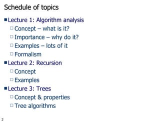
  • 15. Algorithm 1 for Max Subsequence Sum Given A 1 ,…,A n , find the maximum value of A i +A i+ 1 + ··· +A j 0 if the max value is negative int maxSum = 0; for( int i = 0; i < a.size( ); i++ ) for( int j = i; j < a.size( ); j++ ) { int thisSum = 0; for( int k = i; k <= j; k++ ) thisSum += a[ k ]; if( thisSum > maxSum ) maxSum = thisSum; } return maxSum; Time complexity: O  n 3 
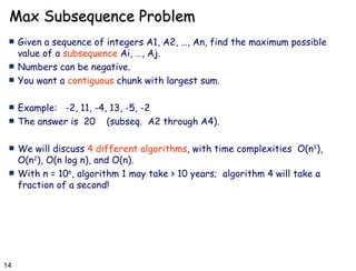
  • 16. Algorithm 2 Idea: Given sum from i to j-1, we can compute the sum from i to j in constant time. This eliminates one nested loop, and reduces the running time to O(n 2 ). into maxSum = 0; for( int i = 0; i < a.size( ); i++ ) int thisSum = 0; for( int j = i; j < a.size( ); j++ ) { thisSum += a[ j ]; if( thisSum > maxSum ) maxSum = thisSum; } return maxSum;
  • 17. Algorithm 3 This algorithm uses divide-and-conquer paradigm. Suppose we split the input sequence at midpoint. The max subsequence is entirely in the left half , entirely in the right half , or it straddles the midpoint . Example: left half | right half 4 -3 5 -2 | -1 2 6 -2 Max in left is 6 (A1 through A3); max in right is 8 (A6 through A7). But straddling max is 11 (A1 thru A7).
  • 18. Algorithm 3 (cont.) Example: left half | right half 4 -3 5 -2 | -1 2 6 -2 Max subsequences in each half found by recursion. How do we find the straddling max subsequence? Key Observation : Left half of the straddling sequence is the max subsequence ending with -2. Right half is the max subsequence beginning with -1. A linear scan lets us compute these in O(n) time.
  • 19. Algorithm 3: Analysis The divide and conquer is best analyzed through recurrence: T(1) = 1 T(n) = 2T(n/2) + O(n) This recurrence solves to T(n) = O(n log n).
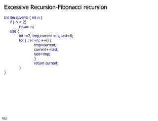
  • 20. Algorithm 4 Time complexity clearly O ( n ) But why does it work? I.e. proof of correctness. 2, 3, -2, 1, -5, 4, 1, -3, 4, -1, 2 int maxSum = 0, thisSum = 0; for( int j = 0; j < a.size( ); j++ ) { thisSum += a[ j ]; if ( thisSum > maxSum ) maxSum = thisSum; else if ( thisSum < 0 ) thisSum = 0; } return maxSum; }
  • 21. Proof of Correctness Max subsequence cannot start or end at a negative Ai. More generally, the max subsequence cannot have a prefix with a negative sum. Ex: -2 11 -4 13 -5 -2 Thus, if we ever find that Ai through Aj sums to < 0, then we can advance i to j+1 Proof. Suppose j is the first index after i when the sum becomes < 0 The max subsequence cannot start at any p between i and j. Because A i through A p-1 is positive, so starting at i would have been even better.
  • 22. Algorithm 4 int maxSum = 0, thisSum = 0; for( int j = 0; j < a.size( ); j++ ) { thisSum += a[ j ]; if ( thisSum > maxSum ) maxSum = thisSum; else if ( thisSum < 0 ) thisSum = 0; } return maxSum The algorithm resets whenever prefix is < 0. Otherwise, it forms new sums and updates maxSum in one pass.
  • 23. Why Efficient Algorithms Matter Suppose N = 10 6 A PC can read/process N records in 1 sec. But if some algorithm does N*N computation, then it takes 1M seconds = 11 days!!! 100 City Traveling Salesman Problem . A supercomputer checking 100 billion tours/sec still requires 10 100 years! Fast factoring algorithms can break encryption schemes. Algorithms research determines what is safe code length. (> 100 digits)
  • 24. How to Measure Algorithm Performance What metric should be used to judge algorithms? Length of the program (lines of code) Ease of programming (bugs, maintenance) Memory required Running time Running time is the dominant standard. Quantifiable and easy to compare Often the critical bottleneck
  • 25. Abstraction An algorithm may run differently depending on: the hardware platform (PC, Cray, Sun) the programming language (C, Java, C++) the programmer (you, me, Bill Joy) While different in detail, all hardware and programming models are equivalent in some sense: Turing machines . It suffices to count basic operations. Crude but valuable measure of algorithm’s performance as a function of input size .
  • 26. Average, Best, and Worst-Case On which input instances should the algorithm’s performance be judged? Average case: Real world distributions difficult to predict Best case: Seems unrealistic Worst case: Gives an absolute guarantee We will use the worst-case measure.
  • 27. Examples Vector addition Z = A+B for (int i=0; i<n; i++) Z[i] = A[i] + B[i]; T(n) = c n Vector (inner) multiplication z =A*B z = 0; for (int i=0; i<n; i++) z = z + A[i]*B[i]; T(n) = c’ + c 1 n
  • 28. Examples Vector (outer) multiplication Z = A*B T for (int i=0; i<n; i++) for (int j=0; j<n; j++) Z[i,j] = A[i] * B[j]; T(n) = c 2 n 2 ; A program does all the above T(n) = c 0 + c 1 n + c 2 n 2 ;
  • 29. Simplifying the Bound T(n) = c k n k + c k-1 n k-1 + c k-2 n k-2 + … + c 1 n + c o too complicated too many terms Difficult to compare two expressions, each with 10 or 20 terms Do we really need that many terms?
  • 30. Simplifications Keep just one term! the fastest growing term (dominates the runtime) No constant coefficients are kept Constant coefficients affected by machines, languages, etc. Asymtotic behavior (as n gets large) is determined entirely by the leading term. Example . T(n) = 10 n 3 + n 2 + 40n + 800 If n = 1,000, then T(n) = 10,001,040,800 error is 0.01% if we drop all but the n 3 term In an assembly line the slowest worker determines the throughput rate
  • 31. Simplification Drop the constant coefficient Does not effect the relative order
  • 32. Simplification The faster growing term (such as 2 n ) eventually will outgrow the slower growing terms (e.g., 1000 n) no matter what their coefficients! Put another way, given a certain increase in allocated time, a higher order algorithm will not reap the benefit by solving much larger problem
  • 33. Complexity and Tractability Assume the computer does 1 billion ops per sec.
  • 34. 2 n n 2 n log n n log n log n n n log n n 2 n 3 n 3 2 n
  • 35. Another View More resources (time and/or processing power) translate into large problems solved if complexity is low 1.3 13 10 2 n 2.2 22 10 N 3 3.2 45 14 5n 2 10 10 1 1000n 10 100 10 100n Increase in Problem size Problem size solved in 10 4 sec Problem size solved in 10 3 sec T(n)
  • 36. Asymptotics They all have the same “growth” rate
  • 37. Caveats Follow the spirit, not the letter a 100n algorithm is more expensive than n 2 algorithm when n < 100 Other considerations: a program used only a few times a program run on small data sets ease of coding, porting, maintenance memory requirements
  • 38. Asymptotic Notations Big-O, “bounded above by”: T(n) = O(f(n)) For some c and N, T(n)  c·f(n) whenever n > N. Big-Omega, “bounded below by”: T(n) =  (f(n)) For some c>0 and N, T(n)  c·f(n) whenever n > N. Same as f(n) = O(T(n)). Big-Theta, “bounded above and below”: T(n) =  (f(n)) T(n) = O(f(n)) and also T(n) =  (f(n)) Little-o, “strictly bounded above”: T(n) = o(f(n)) T(n)/f(n)  0 as n  
  • 39. By Pictures Big-Oh (most commonly used) bounded above Big-Omega bounded below Big-Theta exactly Small-o not as expensive as ...
  • 42. Summary (Why O(n)?) T(n) = c k n k + c k-1 n k-1 + c k-2 n k-2 + … + c 1 n + c o Too complicated O(n k ) a single term with constant coefficient dropped Much simpler, extra terms and coefficients do not matter asymptotically Other criteria hard to quantify
  • 43. Runtime Analysis Useful rules simple statements (read, write, assign) O(1) (constant) simple operations (+ - * / == > >= < <= O(1) sequence of simple statements/operations rule of sums for, do, while loops rules of products
  • 44. Runtime Analysis (cont.) Two important rules Rule of sums if you do a number of operations in sequence, the runtime is dominated by the most expensive operation Rule of products if you repeat an operation a number of times, the total runtime is the runtime of the operation multiplied by the iteration count
  • 45. Runtime Analysis (cont.) if (cond) then O(1) body 1 T 1 (n) else body 2 T 2 (n) endif T(n) = O(max (T 1 (n), T 2 (n))
  • 46. Runtime Analysis (cont.) Method calls A calls B B calls C etc. A sequence of operations when call sequences are flattened T(n) = max(T A (n), T B (n), T C (n))
  • 47. Example for (i=1; i<n; i++) if A(i) > maxVal then maxVal= A(i); maxPos= i; Asymptotic Complexity: O(n)
  • 48. Example for (i=1; i<n-1; i++) for (j=n; j>= i+1; j--) if (A(j-1) > A(j)) then temp = A(j-1); A(j-1) = A(j); A(j) = tmp; endif endfor endfor Asymptotic Complexity is O(n 2 )
  • 49. Run Time for Recursive Programs T(n) is defined recursively in terms of T(k), k<n The recurrence relations allow T(n) to be “unwound” recursively into some base cases (e.g., T(0) or T(1)). Examples: Factorial Hanoi towers
  • 50. Example: Factorial int factorial (int n) { if (n<=1) return 1; else return n * factorial(n-1); } factorial (n) = n*n-1*n-2* … *1 n * factorial(n-1) n-1 * factorial(n-2) n-2 * factorial(n-3) … 2 *factorial(1) T(n) T(n-1) T(n-2) T(1)
  • 51. Example: Factorial (cont.) int factorial1(int n) { if (n<=1) return 1; else { fact = 1; for (k=2;k<=n;k++) fact *= k; return fact; } } Both algorithms are O(n).
  • 52. Example: Hanoi Towers Hanoi(n,A,B,C) = Hanoi(n-1,A,C,B)+Hanoi(1,A,B,C)+Hanoi(n-1,C,B,A)
  • 53. // Early-terminating version of selection sort bool sorted = false; !sorted && sorted = true; else sorted = false; // out of order Worst Case Best Case template<class T> void SelectionSort(T a[], int n) { for (int size=n; (size>1); size--) { int pos = 0; // find largest for (int i = 1; i < size; i++) if (a[pos] <= a[i]) pos = i; Swap(a[pos], a[size - 1]); } } Worst Case, Best Case, and Average Case
  • 54. T(N)=6N+4 : n0=4 and c=7, f(N)=N T(N)=6N+4 <= c f(N) = 7N for N>=4 7N+4 = O(N) 15N+20 = O(N) N 2 =O(N)? N log N = O(N)? N log N = O(N 2 )? T(N) f(N) c f(N) n 0 T(N)=O(f(N)) N 2 = O(N log N)? N 10 = O(2 N )? 6N + 4 = W(N) ? 7N? N+4 ? N 2 ? N log N? N log N = W(N 2 )? 3 = O(1) 1000000=O(1) Sum i = O(N)?
  • 55. An Analogy: Cooking Recipes Algorithms are detailed and precise instructions. Example: bake a chocolate mousse cake. Convert raw ingredients into processed output. Hardware (PC, supercomputer vs. oven, stove) Pots, pans, pantry are data structures. Interplay of hardware and algorithms Different recipes for oven, stove, microwave etc. New advances. New models: clusters, Internet, workstations Microwave cooking, 5-minute recipes, refrigeration
  • 56. Lecture 2 - Recursion
  • 57. What is Recursion? Recursion is when a function either directly or indirectly makes a call to itself. Recursion is a powerful problem solving tool. Many mathematical functions and algorithms are most easily expressed using recursion.
  • 58. How does it work? Functions are implemented using an internal stack of activation records . Each time a function is called a new activation record is pushed on the stack. When a function returns, the stack is popped and the activation record of the calling method is on top of the stack.
  • 59. How does it work? (cont.) The function being called, and whose activation record is being pushed on the stack, can be different from the calling function (e.g., when main calls a function). The function being called can be a different instance of the calling subprogram. Each instance of the function has its own parameters and local variables.
  • 60. Example Many mathematical functions are defined recursively. For example, the factorial function: N! = N * (N-1)! for N>0 0! = 1 We have defined factorial in terms of a smaller (or simpler) instance of itself. We must also define a base case or stopping condition.
  • 61. Recursive Function Call A recursive call is a function call in which the called function is the same as the one making the call. We must avoid making an infinite sequence of function calls (infinite recursion).
  • 62. Finding a Recursive Solution Each successive recursive call should bring you closer to a situation in which the answer is known. general (recursive) case A case for which the answer is known (and can be expressed without recursion) is called a base case .
  • 63. General format for many recursive functions if (some conditions for which answer is known) // base case solution statement else // general case recursive function call
  • 64. Tail Recursion Use only one recursive call at the end of a function void tail (int i) { if (i > 0) { System.out.print( i+ “ ”); tail(i – 1); } } void iterativetail(int i) { for ( ; i > 0; i--) System.out.print( i+ “ ”); }
  • 65. NonTail Recursion void nonTail (int i) { if (i > 0) { nonTail(i – 1); System.out.print( i+ “ ”); nonTail(i – 1); } }
  • 66. Indirect recursion Receive( buffer ) while buffer is not filled up If information is still incoming get a char and store it in buffer; else exit(); decode(buffer); Decode(buffer) decode information in buffer; store(buffer); Store(buffer) transfer information from buffer to file; receive(buffer);
  • 67. Nested recursion h(n) { 0 if n=0 h(n) ={ n if n>4 h(n) { h(2+h(2n)) if n <=4
  • 68. Writing a recursive function to find n factorial DISCUSSION The function call Factorial(4) should have value 24, because that is 4 * 3 * 2 * 1 . For a situation in which the answer is known, the value of 0! is 1. So our base case could be along the lines of if ( number == 0 ) return 1;
  • 69. Writing a recursive function to find Factorial(n) Now for the general case . . . The value of Factorial(n) can be written as n * the product of the numbers from (n - 1) to 1, that is, n * (n - 1) * . . . * 1 or, n * Factorial(n - 1) And notice that the recursive call Factorial(n - 1) gets us “closer” to the base case of Factorial(0).
  • 70. Recursive Function Example: Factorial Problem: calculate n! (n factorial) n! = 1 if n = 0 n! = 1 * 2 * 3 *...* n if n > 0 Recursively: if n = 0 , then n! = 1 if n > 0, then n! = n * ( n-1 ) !
  • 71. Factorial Function int RecFactorial( /* in */ int n) // Calculates n factorial, n! // Precondition: n is a non-negative // integer { if ( n <= 0 ) then return 1 else return n * RecFa ctorial ( n-1 ) }
  • 72. 1 int fact(int n) 2 { 3 if ( n <= 0 ) then 4 return 1; 5 else 6 return n*fact(n-1); 7 } main(...) { ... 20 System.out.print( (fact(3)); ... returns 6 to main()
  • 73. Exponentiation base exponent e.g. 5 3 Could be written as a function Power(base, exp)
  • 74. Can we write it recursively? b e = b * b (e-1) What’s the limiting case? When e = 0 we have b 0 which always equals? 1
  • 75. Another Recursive Function 1 function Power returnsa Num(base, exp) 2 // Computes the value of Base Exp 3 // Pre: exp is a non-negative integer 4 if ( exp = 0 ) then 5 returns 1 6 else 7 returns base * Power (base, exp-1 ) 8 endif 9 endfunction Power x N = x * x N -1 for N >0 x 0 = 1 main(...) { ... 20 cout << (Power(2,3)); ...
  • 76. A man has an infant male-female pair of rabbits in a hutch entirely surrounded by a wall. We wish to know how many rabbits can be bred from this pair in one year, if the nature of the rabbits is such that every month they breed one other male-female pair which begins to breed in the second month after their birth. Assume that no rabbits die during the year. The Puzzle
  • 77. A Tree Diagram for Fibonacci’s Puzzle
  • 78. Observations The number of rabbits at the beginning of any month equals the number of rabbits of the previous month plus the number of new pairs . The number of new pairs at the beginning of a month equals the number of pairs two months ago . One gets the sequence: 1, 1, 2, 3, 5, 8, 13, 21, 34, 55, 89, … 233
  • 79. Fibonacci sequence Recursive definition f(1) = 1 f(2) = 1 f(n) = f(n-1) + f(n-2)
  • 80. Fibonacci Number Sequence if n = 1, then Fib(n) = 1 if n = 2, then Fib(n) = 1 if n > 2, then Fib(n) = Fib(n-2) + Fib(n-1) Numbers in the series: 1, 1, 2, 3, 5, 8, 13, 21, 34, ... A More Complex Recursive Function
  • 81. Fibonacci Sequence Function function Fib returnsaNum (n) // Calculates the nth Fibonacci number // Precondition: N is a positive integer if ( (n = 1) OR (n = 2) ) then returns 1 else returns Fib ( n-2 ) + Fib ( n-1 ) endif endfunction //Fibonacci
  • 82. Tracing with Multiple Recursive Calls Main Algorithm: answer <- Fib(5)
  • 83. Tracing with Multiple Recursive Calls Main Algorithm: answer <- Fib(5) Fib(5): Fib returns Fib(3) + Fib(4)
  • 84. Tracing with Multiple Recursive Calls Main Algorithm: answer <- Fib(5) Fib(5): Fib returns Fib(3) + Fib(4) Fib(3): Fib returns Fib(1) + Fib(2)
  • 85. Tracing with Multiple Recursive Calls Main Algorithm: answer <- Fib(5) Fib(5): Fib returns Fib(3) + Fib(4) Fib(3): Fib returns Fib(1) + Fib(2) Fib(1): Fib returns 1
  • 86. Tracing with Multiple Recursive Calls Main Algorithm: answer <- Fib(5) Fib(5): Fib returns Fib(3) + Fib(4) Fib(3): Fib returns 1 + Fib(2)
  • 87. Tracing with Multiple Recursive Calls Main Algorithm: answer <- Fib(5) Fib(5): Fib returns Fib(3) + Fib(4) Fib(3): Fib returns 1 + Fib(2) Fib(2): Fib returns 1
  • 88. Tracing with Multiple Recursive Calls Main Algorithm: answer <- Fib(5) Fib(5): Fib returns Fib(3) + Fib(4) Fib(3): Fib returns 1 + 1
  • 89. Tracing with Multiple Recursive Calls Main Algorithm: answer <- Fib(5) Fib(5): Fib returns 2 + Fib(4)
  • 90. Tracing with Multiple Recursive Calls Main Algorithm: answer <- Fib(5) Fib(5): Fib returns 2 + Fib(4) Fib(4): Fib returns Fib(2) + Fib(3)
  • 91. Tracing with Multiple Recursive Calls Main Algorithm: answer <- Fib(5) Fib(5): Fib returns 2 + Fib(4) Fib(4): Fib returns Fib(2) + Fib(3) Fib(2): Fib returns 1
  • 92. Tracing with Multiple Recursive Calls Main Algorithm: answer <- Fib(5) Fib(5): Fib returns 2 + Fib(4) Fib(4): Fib returns 1 + Fib(3)
  • 93. Tracing with Multiple Recursive Calls Main Algorithm: answer <- Fib(5) Fib(5): Fib returns 2 + Fib(4) Fib(4): Fib returns 1 + Fib(3) Fib(3): Fib returns Fib(1) + Fib(2)
  • 94. Tracing with Multiple Recursive Calls Main Algorithm: answer <- Fib(5) Fib(5): Fib returns 2 + Fib(4) Fib(4): Fib returns 1 + Fib(3) Fib(3): Fib returns Fib(1) + Fib(2) Fib(1): Fib returns 1
  • 95. Tracing with Multiple Recursive Calls Main Algorithm: answer <- Fib(5) Fib(5): Fib returns 2 + Fib(4) Fib(4): Fib returns 1 + Fib(3) Fib(3): Fib returns 1 + Fib(2)
  • 96. Tracing with Multiple Recursive Calls Main Algorithm: answer <- Fib(5) Fib(5): Fib returns 2 + Fib(4) Fib(4): Fib returns 1 + Fib(3) Fib(3): Fib returns 1 + Fib(2) Fib(2): Fib returns 1
  • 97. Tracing with Multiple Recursive Calls Main Algorithm: answer <- Fib(5) Fib(5): Fib returns 2 + Fib(4) Fib(4): Fib returns 1 + Fib(3) Fib(3): Fib returns 1 + 1
  • 98. Tracing with Multiple Recursive Calls Main Algorithm: answer <- Fib(5) Fib(5): Fib returns 2 + Fib(4) Fib(4): Fib returns 1 + 2
  • 99. Tracing with Multiple Recursive Calls Main Algorithm: answer <- Fib(5) Fib(5): Fib returns 2 + 3
  • 100. Tracing with Multiple Recursive Calls Main Algorithm: answer <- 5
  • 101. Fib(5) 15 calls to Fib to find the 5th Fibonacci number!!! Fib(3) Fib(4) Fib(3) Fib(2) Fib(2) Fib(1) Fib(1) Fib(0) Fib(1) Fib(0) Fib(2) Fib(1) Fib(1) Fib(0)
  • 102. Excessive Recursion-Fibonacci recursion Int iterativeFib ( int n ) if ( n < 2) return n; else { int i=2, tmp,current = 1, last=0; for ( ; i<=n; ++i) { tmp=current; current+=last; last=tmp; } return current; } }
  • 103.  
  • 104.  
  • 105. Rules of Recursion First two fundamental rules of recursion: Base cases: Always have at least one case that can be solved without using recursion. Make progress: Any recursive call must make progress towards the base case.
  • 106. Rules of Recursion Third fundamental rule of recursion: “ You gotta believe”: Always assume that the recursive call works.
  • 107. Rules of Recursion Fourth fundamental rule of recursion: Compound interest rule: Never duplicate work by solving the same instance of a problem in separate recursive calls.
  • 108. Towers of Hanoi The puzzle consisted of N disks and three poles: A (the source), B (the destination), and C (the spare)
  • 109. Towers of Hanoi B C A
  • 110. Towers of Hanoi B C A
  • 111. Towers of Hanoi B C A
  • 112. Towers of Hanoi B C A
  • 113. Towers of Hanoi B C A
  • 114. Towers of Hanoi B C A
  • 115. Towers of Hanoi B C A
  • 116. Towers of Hanoi B C A
  • 117. Towers of Hanoi A pseudocode description of the solution is: Towers(Count, Source, Dest, Spare) if (Count is 1) Move the disk directly from Source to Dest else { Solve Towers(Count-1, Source, Spare, Dest) Solve Towers(1, Source, Dest, Spare) Solve Towers(Count-1, Spare, Dest, Source) }
  • 118. Towers of Hanoi void solveTowers( int count, char source, char dest, char spare){ if (count == 1) cout<<“Move disk from pole “ << source << &quot; to pole &quot; << destination <<endl; else { towers(count-1, source, spare, destination); towers(1, source, destination, spare); towers(count-1, spare, destination, source); }//end if }//end solveTowers
  • 119. Recall that . . . Recursion occurs when a function calls itself (directly or indirectly). Recursion can be used in place of iteration (looping). Some functions can be written more easily using recursion.
  • 120. Pascal Triangle (Is this recursive?)
  • 121. Pascal Triangle The combinations of n items taken r at a time . For example: three items:    a    b    c taken 2 at a time:    ab    ac    bc Thus there are three combinations of 3 items taken 2 at a time. In General:    C(n,r) = n!/(r!(n-r)!)     Obviously you can calculate C(n,r) using factorials.
  • 122. Pascal Triangle This leads to Pascal Triangle: n     0                             1              1                       1       1              2                    1     2      1              3                1     3      3     1              4            1     4      6      4    1              5        1     5      10     10    5    1 This can also be written:             r     0    1    2    3     4    5         n  0     1             1     1     1              2     1     2    1              3     1     3    3    1             4     1     4    6    4    1              5     1     5   10  10    5    1
  • 123. Pascal Triangle Note from Pascal's Triangle that:     C(n,r) = C(n-1, r-1) + C(n-1,r) This leads to the recurrence for nonnegative r and n, C(n,r) =               1             if r = 0 or r = n,                            0             if r > n,                             C(n-1, r-1) + C(n-1,r)     otherwise.
  • 124. Pascal Triangle This immediately leads to the recursive function for combinations:   int C(int n, int r) {   if((r == 0) || (r == n))      return 1;   else if(r > n)       return 0;   else        return C(n-1, r-1) + C(n-1, r);     }
  • 125. What is the value of rose(25) ? int rose (int n) { if ( n == 1 ) // base case return 0; else // general case return ( 1 + rose ( n / 2 ) ); }
  • 126. Finding the value of rose(25) rose(25) the original call = 1 + rose(12) first recursive call = 1 + ( 1 + rose(6) ) second recursive call = 1 + ( 1 + ( 1 + rose(3) ) ) third recursive call = 1 + ( 1 + ( 1 + (1 + rose(1) ) ) ) fourth recursive call = 1 + 1 + 1 + 1 + 0 = 4
  • 127. Writing recursive functions There must be at least one base case, and at least one general (recursive) case. The general case should bring you “closer” to the base case. The parameter(s) in the recursive call cannot all be the same as the formal parameters in the heading. Otherwise, infinite recursion would occur. In function rose( ) , the base case occurred when (n == 1) was true. The general case brought us a step closer to the base case, because in the general case the call was to rose(n/2) , and the argument n/2 was closer to 1 (than n was).
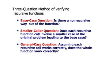
  • 128. Three-Question Method of verifying recursive functions Base-Case Question: Is there a nonrecursive way out of the function? Smaller-Caller Question: Does each recursive function call involve a smaller case of the original problem leading to the base case? General-Case Question: Assuming each recursive call works correctly, does the whole function work correctly?
  • 129. Guidelines for writing recursive functions 1. Get an exact definition of the problem to be solved. 2. Determine the size of the problem to be solved on this call to the function. On the initial call, the size of the whole problem is expressed by the actual parameter(s). 3. Identify and solve the base case(s) which have non-recursive solutions. 4. Identify and solve the general case(s) in terms of smaller (recursive) cases of the same problem.
  • 130. struct ListType { int length ; // number of elements in the list int info[ MAX_ITEMS ] ; } ; ListType list ; struct ListType
  • 131. Recursive function to determine if value is in list PROTOTYPE bool ValueInList( ListType list , int value , int startIndex ) Already searched Needs to be searched index of current element to examine 74 36 . . . 95 list[0] [1] [startIndex] 75 29 47 . . . [length -1]
  • 132. bool ValueInList ( ListType list , int value , int startIndex ) // Searches list for value between positions startIndex // and list.length-1 { if ( list.info[startIndex] == value ) // one base case return true ; else if (startIndex == list.length -1 ) // another base case return false ; else // general case return ValueInList( list, value, startIndex + 1 ) ; }
  • 133. “ Why use recursion?” Many solutions could have been written without recursion, by using iteration instead. The iterative solution uses a loop, and the recursive solution uses an if statement. However, for certain problems the recursive solution is the most natural solution. This often occurs when pointer variables are used.
  • 134. When to Use Recursion If the problem is recursive in nature therefore it is likely the a recursive algorithm will be preferable and will be less complex If running times of recursive and non-recursive algorithms are hardly perceivable, recursive version is better If both recursive and non-recursive algorithms have the same development complexity, a non-recursive version should be preferred A third alternative in some problems is to use table-driven techniques Sometimes we know that we will not use the only a few values of a particular function If this is the case an implementation using a table would probably suffice and the performance will be better int factorial[8] = {1, 1, 2, 6, 24, 120, 720, 5040};
  • 135. Use a recursive solution when: The depth of recursive calls is relatively “shallow” compared to the size of the problem. The recursive version does about the same amount of work as the nonrecursive version. The recursive version is shorter and simpler than the nonrecursive solution. SHALLOW DEPTH EFFICIENCY CLARITY
  • 136. Lecture 3 – Binary Trees
  • 137. Why Trees? Limitations of Arrays Linked lists Stacks Queues
  • 138. Trees: Recursive Definition A tree is a collection of nodes. The collection can be empty, or consist of a “root” node R. There is a “directed edge” from R to the root of each subtree. The root of each subtree is a “child” of R . R is the “parent” of each subtree root.
  • 139. Trees: Recursive Definition (cont.) ROOT OF TREE T T1 T2 T3 T4 T5 SUBTREES
  • 140. Trees: An Example A B C D E F G H I
  • 141. Trees: More Definitions Nodes with no children are leaves : (C,E,F,H,I). Nodes with the same parents are siblings : (B,C,D,E) and (G,H). A path from node n to node m is the sequence of directed edges from n to m . A length of a path is the number of edges in the path
  • 142. Trees: More Definitions (cont.) The level/depth of node n is the length of the path from the root to n . The level of the root is 0. The height/depth of a tree is equal to the maximum level of a node in the tree. The height of a node n is the length of the longest path from n to a leaf. The height of a leaf node is 0. The height of a tree is equal to the height of the root node.
  • 143. Binary Trees – A Informal Definition A binary tree is a tree in which no node can have more than two children. Each node has 0, 1, or 2 children In this case we can keep direct links to the children: struct TreeNode { Object element; TreeNode *left_child; TreeNode *right_child; };
  • 144. Binary Trees – Formal Definition A binary tree is a structure that contains no nodes, or is comprised of three disjoint sets of nodes: a root a binary tree called its left subtree a binary tree called its right subtree A binary tree that contains no nodes is called empty
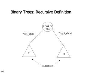
  • 145. Binary Trees: Recursive Definition ROOT OF TREE T T1 T2 SUBTREES *left_child *right_child
  • 146. Differences Between A Tree & A Binary Tree No node in a binary tree may have more than 2 children, whereas there is no limit on the number of children of a node in a tree. The subtrees of a binary tree are ordered; those of a tree are not ordered.
  • 147. Differences Between A Tree & A Binary Tree (cont.) The subtrees of a binary tree are ordered; those of a tree are not ordered Are different when viewed as binary trees Are the same when viewed as trees a b a b
  • 148. Internal and External Nodes Because in a binary tree all the nodes must have the same number of children we are forced to change the concepts slightly We say that all internal nodes have two children External nodes have no children internal node external node
  • 149. Recursive definition of a Binary Tree Most of concepts related to binary trees can be explained recursive For instance, A binary tree is: An external node , or An internal node connected to a left binary tree and a right binary tree (called left and right subtrees) In programming terms we can see that our definition for a linked list (singly) can be modified to have two links from each node instead of one.
  • 150. Property2 : a unique path exists from the root to every other node What is a binary tree? (cont.)
  • 151. Mathematical Properties of Binary Trees Let's us look at some important mathematical properties of binary trees A good understanding of these properties will help the understanding of the performance of algorithms that process trees Some of the properties we'll describe relate also the structural properties of these trees. This is the case because performance characteristics of many algorithms depend on these structural properties and not only the number of nodes.
  • 152. Minimum Number Of Nodes Minimum number of nodes in a binary tree whose height is h . At least one node at each level. minimum number of nodes is h + 1
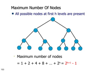
  • 153. Maximum Number Of Nodes All possible nodes at first h levels are present Maximum number of nodes = 1 + 2 + 4 + 8 + … + 2 h = 2 h+1 - 1
  • 154. Number of Nodes & Height Let n be the number of nodes in a binary tree whose height is h . h + 1 <= n <= 2 h+1 – 1 log 2 (n+1)-1 <= h <= n -1 The max height of a tree with N nodes is N - 1 (same as a linked list) The min height of a tree with N nodes is log(N+1)-1
  • 155. Relationship Between Number of Nodes (Internal - External) A binary tree with N internal nodes has N+1 external nodes Let's try to prove this using induction...
  • 156. Number of edges A binary tree with N internal nodes has 2N edges Let's try to prove this using induction...
  • 157. Number of edges A binary tree with N nodes (internal and external) has N-1 edges Let's try to prove this using induction...
  • 158. Binary Tree Representation Array representation Linked representation
  • 159. Binary Trees Full binary tree : All internal nodes have two children. Complete binary tree : All leaves have the same level All internal nodes have two children
  • 160. Node Number Properties Parent of node i is node i/2 But node 1 is the root and has no parent Left child of node i is node 2i But if 2i > n , node i has no left child Right child of node i is node 2i+1 But if 2i+1 > n , node i has no right child Complete binary tree 1 2 3 4 5 6 7 8 9 10 11 12 13 14 15
  • 161. Full Binary Tree With n Nodes Start with a complete binary tree that has at least n nodes. Number the nodes as described earlier. The binary tree defined by the nodes numbered 1 through n is the unique n node full binary tree. Full binary tree with 11 nodes 1 2 3 4 5 6 7 8 9 10 11 12 13 14 15
  • 162. Array Representation Number the nodes using the numbering scheme for a full binary tree Store the node numbered i in tree[i] a b c d e f g h i j 1 2 3 4 6 7 8 9 b a c d e f g h i j 1 2 3 4 5 6 7 8 9 10 tree[] 0 5 10
  • 163. Right-Skewed Binary Tree An n node binary tree needs an array whose length is between n+1 and 2 n If h = n-1 then skewed binary tree a b 1 3 c 7 d 15 tree[] 0 5 10 a - b - - - c - - - - - - - 15 d
  • 164. Array Representation (cont.) Each tree node is represented as a struct Struct TreeNode { object element; int child1; int child2; … int childn; }; Struct TreeNode tree[100];
  • 165. Linked Representation Each tree node is represented as an object whose data type is TreeNode The space required by an n node binary tree is n * (space required by one node)
  • 166. Trees: Linked representation Implementation 1 struct TreeNode { Object element; TreeNode *child1; TreeNode *child2; . . . TreeNode *childn; }; Each node contains a link to all of its children. This isn’t a good idea, because a node can have an arbitrary number of children!
  • 167. struct TreeNode { Object element; TreeNode *child1; TreeNode *sibling; }; Each node contain a link to its first child and a link to its next sibling. This is a better idea. Trees: Linked representation Implementation 2
  • 168. Implementation 2: Example / The downward links are to the first child; the horizontal links are to the next sibling. / / / / A / B F / C D E / G H / I /
  • 169. Binary Trees A binary tree is a tree whose nodes have at most two offspring Example struct nodeType { object element; struct nodeType *left, *right; }; struct nodeType *tree;
  • 170. Linked Representation Example a c b d f e g h leftChild element rightChild root
  • 171. Some Binary Tree Operations • Determine the height. • Determine the number of nodes. • Make a clone. • Determine if two binary trees are clones. • Display the binary tree. • Evaluate the arithmetic expression represented by a binary tree. • Obtain the infix form of an expression. • Obtain the prefix form of an expression. • Obtain the postfix form of an expression.
  • 172. CS122 Algorithms and Data Structures Week 7: Binary Search Trees Binary Expression Trees
  • 173. Uses for Binary Trees… -- Binary Search Trees Use for storing and retrieving information Insert, delete, and search faster than with a linked list Idea: Store information in an ordered way (keys)
  • 174. A Property of Binary Search Trees The key of the root is larger than any key in the left subtree The key of the root is smaller than any key in the right subtree Note: Duplicated keys are not allowed
  • 175. A Property of Binary Search Tree ROOT OF TREE T T1 T2 SUBTREES *left_child *right_child X All nodes in T1 have keys < X. All nodes in T2 have keys > X.
  • 176. Binary Search Trees in C++ We will use two classes: The class BinaryNode simply constructs individual nodes in the tree. The class BinarySearchTree maintains a pointer to the root of the binary search tree and includes methods for inserting and removing nodes.
  • 177. Search Operation BinaryNode *search (const int &x, BinaryNode *t) { if ( t == NULL ) return NULL; if (x == t->key) return t; // Match if ( x < t->key ) return search( x, t->left ); else // t ->key < x return search( x, t->right ); }
  • 178. FindMin Operation BinaryNode* findMin (BinaryNode *t) { if ( t == NULL ) return NULL; if ( t -> left == NULL ) return t; return findMin (t -> left); } This method returns a pointer to the node containing the smallest element in the tree.
  • 179. FindMax Operation BinaryNode* findMax (BinaryNode *t) { if ( t == NULL ) return NULL; if ( t -> right == NULL ) return t; return findMax (t -> right); } This function returns a pointer to the node containing the largest element in the tree.
  • 180. Insert Operation To insert X into a tree T, proceed down the tree as you would with a find. If X is found, do nothing. Otherwise insert X at the last spot on the path that has been traversed.
  • 181. Insert Operation (cont.) void BinarySearchTree insert (const int &x, BinaryNode *&t) const { if (t == NULL) t = new BinaryNode (x, NULL, NULL); else if (x < t->key) insert(x, t->left); else if( t->key < x) insert(x, t->right); else ; // Duplicate entry; do nothing } Note the pointer t is passed using call by reference.
  • 182. Removal Operation If the node to be removed is a leaf, it can be deleted immediately. If the node has one child , the node can be deleted after its parent adjusts a link to bypass the deleted node.
  • 183. If the node to be removed has two children , the general strategy is to replace the data of this node with the smallest key of the right subtree . Then the node with the smallest data is now removed (this case is easy since this node cannot have two children). Removal Operation (cont.)
  • 184. Removal Operation (cont.) void remove (const int &x, BinaryNode* &t) const { if ( t == NULL ) return; // key is not found; do nothing if ( t->key == x) { if( t->left != NULL && t->right != NULL ) { // Two children t->key = findMin( t->right )->key; remove( t->key, t->right ); } else { // One child BinaryNode *oldNode = t; t = ( t->left != NULL ) ? t->left : t->right; delete oldNode; } } else { // Two recursive calls if ( x < t->key ) remove( x, t->left ); else if( t->key < x ) remove( x, t->right ); } }
  • 188. Balancing a binary tree A binary tree is height-balanced or simply balanced if the difference in height of both the subtrees is either zero or one Perfectly balanced if all leaves are to be found on one level or two levels.
  • 190. Analysis The running time of these operations is O(lv) , where lv is the level of the node containing the accessed item. What is the average level of the nodes in a binary search tree? It depends on how well balanced the tree is.
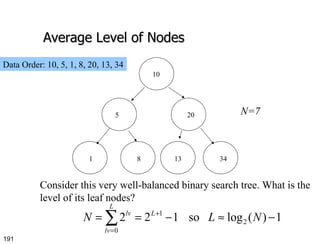
  • 191. Average Level of Nodes 10 5 20 1 8 13 34 Consider this very well-balanced binary search tree. What is the level of its leaf nodes? N=7 Data Order: 10, 5, 1, 8, 20, 13, 34
  • 192. A Better Analysis The analysis on the previous slide was for a particularly well-balanced binary search tree. However, not all binary search trees will be this well balanced. In particular, binary search trees are created via insertions of data. Depending on the order of the data, various trees will emerge.
  • 193. Effect of Data Order Obtained if data is 4, 3, 2 1 Obtained if data is 1, 2, 3, 4 Note in these cases the average depth of nodes is about N/2 , not log(N)!
  • 194. Depth of Nodes In the best case the depth will be about O(log N). In the worst case, if the data are already ordered, the depth will be about O(N).
  • 195. Effects of Data Order… So, if the input data are randomly ordered, what is the average depth of the nodes? The analysis is beyond the scope of this course, but it can be shown that the average depth is O(log N), which is a very nice result.
  • 196. Summary In this lecture we showed that, for an average binary search tree, the average depth of the nodes is O(log N). This is quite amazing, indicating that the bad situations, which are O(N), don’t occur very often. However, for those who are still concerned about the very bad situations, we can try to “balance” the trees.
  • 197. Uses for Binary Trees… -- Binary Expression Trees Binary trees are a good way to express arithmetic expressions. The leaves are operands and the other nodes are operators. The left and right subtrees of an operator node represent subexpressions that must be evaluated before applying the operator at the root of the subtree.
  • 198. Binary Expression Trees: Examples a + b - a (a + b) * (c – d) / (e + f) + a b - a / + a b - c d + e f * /
  • 199. Merits of Binary Tree Form Left and right operands are easy to visualize Code optimization algorithms work with the binary tree form of an expression Simple recursive evaluation of expression + a b - c d + e f * /
  • 200. Levels Indicate Precedence The levels of the nodes in the tree indicate their relative precedence of evaluation (we do not need parentheses to indicate precedence). Operations at lower levels of the tree are evaluated later than those at higher levels. The operation at the root is always the last operation performed.
  • 201. A Binary Expression Tree What value does it have? ( 4 + 2 ) * 3 = 18 ‘ *’ ‘ +’ ‘ 4’ ‘ 3’ ‘ 2’
  • 202. Inorder Traversal: (A + H) / (M - Y) ‘ +’ ‘ A’ ‘ H’ ‘ -’ ‘ M’ ‘ Y’ tree Print left subtree first Print right subtree last Print second ‘ /’
  • 203. Inorder Traversal (cont.) a + * b c + * + g * d e f Inorder traversal yields: (a + (b * c)) + (((d * e) + f) * g)
  • 204. Preorder Traversal: / + A H - M Y ‘ +’ ‘ A’ ‘ H’ ‘ -’ ‘ M’ ‘ Y’ tree Print left subtree second Print right subtree last Print first ‘ /’
  • 205. Preorder Traversal (cont.) a + * b c + * + g * d e f Preorder traversal yields: (+ (+ a (* b c)) (* (+ (* d e) f) g))
  • 206. ‘ +’ ‘ A’ ‘ H’ ‘ -’ ‘ M’ ‘ Y’ tree Print left subtree first Print right subtree second Print last Postorder Traversal: A H + M Y - / ‘ /’
  • 207. Postorder Traversal (cont.) a + * b c + * + g * d e f Postorder traversal yields: a b c * + d e * f + g * +
  • 208. Traversals and Expressions Note that the postorder traversal produces the postfix representation of the expression. Inorder traversal produces the infix representation of the expression. Preorder traversal produces a representation that is the same as the way that the programming language Lisp processes arithmetic expressions!
  • 209. Constructing an Expression Tree There is a simple O( N ) stack-based algorithm to convert a postfix expression into an expression tree. Recall we also have an algorithm to convert an infix expression into postfix, so we can also convert an infix expression into an expression tree without difficulty (in O( N ) time).
  • 210. Expression Tree Algorithm Read the postfix expression one symbol at at time: If the symbol is an operand, create a one-node tree and push a pointer to it onto the stack. If the symbol is an operator, pop two tree pointers T1 and T2 from the stack, and form a new tree whose root is the operator, and whose children are T1 and T2. Push the new tree pointer on the stack.
  • 211. Example a b + : Note: These stacks are depicted horizontally. a b + b a
  • 212. Example a b + c d e + : + b a c d e + b a c d e +
  • 213. Example a b + c d e + * : + b a c d e + *
  • 214. Example a b + c d e + * * : + b a c d e + * *