SlideShare a Scribd company logo
PROBABILITY AND STATISTICS
By
Dr. Mamatha S Upadhya
CHAPTER I
Univariate Data Analysis
What is Statistics?
According to Croxten and Cowden “ Statistics is the science which deals
with collection, presentation, analysis and interpretation of numerical
data.”
Why Study Statistics?
some of the functions of statistics can be as follows:
 To present facts in a definite form
 Statistics facilitates comparisons
 Statistics gives guidance in the formulation of suitable policies.
 Statistics can be formulated well in advance for predictions.
 Statistical methods are helpful in formulating, testing hypothesis and
develop new theories.
Application of Statistics in Computer Science
 Machine learning
 Data Science
 Data mining
 Big data
 Artificial intelligence
 Network and Traffic Modelling
 Image Analysis
Descriptive Statistics
Descriptive statistics include graphical and numerical procedures that are used to summarize
data and to transform data into information.
Example: Suppose you want to study average height of the students in a class room. In
descriptive statistics what you would do is you would record the height of all students in a
class then you would find maximum , minimum and average height of the students in a class.
Example : The number of customers who visited a jewellery shop in the last 10 days were-
83, 80, 79, 85, 84, 106, 111, 120, 74, 77
Not much variation in the first five days. High next two days (weekend?). High on the next day
(specific occasion?) ….
Variable: In statistics, the term ‘variable’ is used, only if, the changing characteristics can
be numerically measured. Thus, heights and weights of individuals are variables, as they
can be measured in numerical terms.
Other examples include: price of commodities, income of individuals, household
expenditures, age.
Attribute: Attribute is defined as a characteristic or quality of an object / individual.
The looks of people, their intelligence and aptitude for art and music change from one
individual to the other, they cannot be measured numerically but can be counted, where
as a change in the attribute is only expressed qualitatively as good, excellent or average.
Height: Tall Short
Weight: Fat Medium Thin
What is Data?
Data can be defined as a representation of facts,
concepts, or instructions in a formalized manner, which
should be suitable for communication, interpretation, or
processing by human or electronic machine.
Data is represented with the help of characters such as
alphabets (A-Z, a-z), digits (0-9) or special characters
(+,-,/,*,<,>,= etc.)
It is the raw list of facts that are processed to gain
information.
Qualitative data is the data in which the classification of objects is based on attributes
(quality)
Quantitative data is the type of data which can be measured and expressed
numerically.
Understanding Data
Columns are variables representing name, Gender, age, score, experience.
Rows are representing observations.
Now what type of data are these? First two columns represent Qualitative data and
next three column represent Quantitative data.
Introduction to Statistics and Arithmetic Mean
Examples for quantitative variables
Size of shirt- 39, 40, 42, 50 etc.
Per kilo prices of vegetables- Rs.30, Rs. 35, Rs.40 etc.
Number of colleges in a city- 8, 12, 15 etc.
Height of children- 1.2, 1.23, 1.32 etc.
Examples for qualitative variables
Names of cities – Kanpur, Delhi, Bangalore etc.
Colours of hair- Black, White, Brown, Red etc.
Taste of food – Sweet, Salty, neutral etc.
Performance- Good, Excellent, bad etc.
Data Set: A data set is a collection of observations on one or more variables.
MEASUREMENT SCALES
Measurement: The process of applying numbers to objects
according to a set of rules.
The four level of measurements are: nominal scale, ordinal scale,
interval scale, and ratio scale.
S. S. Stevens (1906 -1973) described the data into different scales
of measurement as nominal, ordinal and cardinal data.
Nominal Scale
The nominal scale is a scale of measurement that is used for identification purposes.
Sometimes known as categorical scale, These numbers have no real meaning and
only act as labels. It helps in differentiating between objects.
Example: For example, number representing on tea shirts of sports person. You
could find one cricketer wearing number 12 and another wearing 85. They only help
us to differentiate the person. The number provides no insight into the player’s
position.
Examples of Nominal Scales
Ordinal Scale
Ordinal Scale involves the ranking or ordering of the observations. The items in this
scale are classified according to the degree of occurrence of the variable. The
attributes on an ordinal scale are usually arranged in ascending or descending order.
It measures the degree of occurrence of the variable. Here, the order of variables is
of prime importance and so is the labeling.
Example: Class ranking :1st , 5th, 16th, 18th,25th,….
Teaching ability : good, average, bad.
Grades of students: A, B, C, D.
Social Status: High, middle, low
Interval Scale
In an Interval Scale numbers used to rank the objects also represents equal increments of the
variable being measured.
Examples: Time ,The difference between 6:00PM and 7:00PM is 1 hour, as is the difference
between 4;00PM and 5:00PM.
Celsius Temperature: The difference between 90 and 70 degrees is a 20 degrees, as is the
difference between 40 and 60 degrees.
Here increments are known, consistent and measurable.
In Interval scale there is no 0 (zero). They do not have “true zero” there occurs arbitrary zero.
There is no such thing as “no temperature”. “no time”
Ratio Scale
Ratio Scale is defined as a variable measurement scale that not only produces the order of
variables but also makes the difference between variables known along with information on
the value of true zero. It is calculated by assuming that the variables have an option for zero,
the difference between the two variables is the same and there is a specific order between the
options.
The best examples of ratio scales are income, savings, weight, height etc.
Note: Quantitative data is usually expressed using either Interval scale or Ratio Scale.
Qualitative Data is expressed using either Nominal Scale or ordinal Scale.
Methods of Data Collection
Data means the raw facts and figures that have been collected. Data can be gathered
by looking through existing sources, conducting experiments or by conducting
surveys. Based on these sources of collections, statistical data may be classified as
primary or secondary.
PRIMARY DATA SECONDARY DATA
Primary data are original
observations collected by the
investigator or his agent for the first
time for any investigation using
methods like surveys, interviews, or
experiments.
The secondary data is the collection of data from
second hand information. This information is
known as, given data is already collected from any
one persons for some purpose, and it available for
the present issues. And mostly these secondary
data’s are not relevant and pure or original data.
Example: Data collection from Government
publications, websites, books, journal articles,
internal records etc.
Formation of Statistical series
Individual series: The data as observed by an investigator is known as individual series.
For example: Marks scored by 10 students:
100, 90, 72, 59, 40, 20, 23, 75, 61,43.
Runs scored by the 11 players of the Indian cricket team in a match are given as follows:
25,65,03,12,35,46,67,56,00,31,17.
Discrete Series: When the data collected are large in number and they are distinct then we can
form a frequency distribution (the number of units associated with each value of the variable).
The number of times a data occurs in a data set is known as the frequency of data.
For example: In a quiz, the marks obtained by 20 students out of 30 are given as:
12,15,15,29,30,21,30,30,15,17,19,15,20,20,16,21,23,24,23,21
Marks obtained in quiz Number of students(Frequency)
12 1
15 4
16 1
17 1
19 1
20 2
21 3
23 2
24 1
29 1
30 3
Total 20
Frequency Distribution Table (Ungrouped)
Grouped series
If the data are large in number, then the discrete series can be further reduced down by grouping
them with the help of class intervals.
Example: following table which represents the height of 200 students of high school.
Grouped Frequency Distribution Table
The first column of the table represents the class interval with a class width of 10. In each class, the
lowest number denotes the lower class limit and the higher number indicates the upper-class limit.
For the class 150-159, the lower class limit is 150 and the upper-class limit is 159. This is known as
grouped frequency distribution.
Height of Students (in cm.) Number of students(Frequency)
130-139 19
140-149 42
150-159 35
160-169 78
170-189 26
Total 200
Continuous Series
There are certain variables which will not have a distinct integer value. For example, weight,
height, etc. In those cases the data will be of continuous type and grouping of those continuous
data is known as “continuous series”.
Example: Height in Centimeters of students: 155.0, 163.3, 155.0, 169.9, 163.9, 148.2,
151.5,128.9, 146.1, 145.2, 156.6, 159.9, 158.0, 153.4, 160.0, 149.3, 154.2, 164.7, 159.0,160.8,
157.1,176.0, 164.4, 170.0, 152.9, 169.3, 159.5,162.4, 173.6, 154.8,158.3,172.5,158.0, 154.0,
172.2, 148.0, 152.4,156.6, 157.7,165.3.
In case of both grouped series and continuous series the class width depends on number of
classes. To find the width of the classes we use the formula:
i=
𝑳−𝑺
𝑲
where i is the class width, L is the largest value of the given data, S is the smallest
value of the given data, K is the number of classes.
i=
𝑳−𝑺
𝑲
=
172.5−145.2
5
=5.46
Now we round this approximate width to a convenient number, say 5.
Heights Number of students
145-150 5
150-155 7
155-160 12
160-165 7
165-170 3
170-175 4
175-180 2
Frequency Distribution or Frequency tables
A systematic presentation of the values taken by a variable and the corresponding frequencies
is called the frequency distribution of that variable. A tabular presentation of the frequency
distribution is called the frequency table.
Frequency distribution are of two types.
(a) discrete frequency distribution
(b) Continuous frequency distribution.
A frequency distribution in which class intervals are considered is known as continuous
frequency distribution. If class intervals are not considered it is a discrete frequency
distribution.
Frequency Distribution or Frequency tables(Contd.)
The difference between the class limits of a class interval is known as the width of the class interval.
In a frequency distribution, the class intervals may be inclusive or exclusive. If a class interval is
such that the lower as well as the upper class limits are included in the same class interval it is
inclusive class interval. If a class interval is such that the lower limit is included in the first class
interval where as the upper class limit is included in the successive class interval it is exclusive class
interval. This method is widely followed in practice.
For example: 10,25,20, 12, 30, 46, 19, 15, 17, 20, 25.
In inclusive class interval 20 will be included in 20-29 and in exclusive class interval 20 will be
included in 20-30 instead of 10-20 interval.
Inclusive Class interval Exclusive Class interval
10-19 5 10-20 5
20-29 4 20-30 4
30-39 1 30-40 1
40-49 1 40-50 1
Example:
Suppose a worker’s wages is Rs. 109.50. He is to be included in class I or the II? Under
such circumstances, it is suggested that inclusive limits of classes be converted into
exclusive limits.
Correction factor=
1
2
110 − 109 =0.5
This is added to the upper limit and subtracted from the lower limit of the class.
Wages in Rs: I
method
100-109 110-119 120-129 130-139 140-149 150-159
Wages in Rs: II
method
101-110 111-120 121-130 131-140 141-150 151-160
Wages in Rs: I
method
99.5-
109.5
109.5-
119.5
119.5-
129.5
129.5-
139.5
139.5-
149.5
149.5-
159.5
Wages in Rs: II
method
100.5-
110.5
110.5-
120.5
120.5-
130.5
130.5-
140.5
140.5-
150.5
150.5-
160.5
Cumulative Frequency Distribution
Cumulative frequency of a given variable or class represents the total frequency of all
previous variables including the variable or the class. i.e the added –up frequencies are
called Cumulative frequency
Class Frequency Cumulative Frequency
10-14 6 6
15-19 11 17
20-24 12 29
25-29 10 39
Example: The following data give the total number of iPods sold by a mail order
company on each of 30 days. Construct a frequency distribution table.
8, 25, 11, 15, 29, 22, 10, 5, 17, 21, 22, 13, 26, 16, 18, 12, 9, 26, 20, 16, 23, 14, 19,
23, 20, 16, 27, 16, 21, 14
Solution: In these data, the minimum value is 5, and the maximum value is 29.
Suppose we decide to group these data using five classes of equal width. Then,
Approximate width of each class = 29 – 5 / 5 = 4.8
Now we round this approximate width to a convenient number, say 5. The lower
limit of the first class can be taken as 5 or any number less than 5.
Frequency Distribution for the Data on iPods Sold
i Pods Sold Frequency
5-9 /// 3
10-14 ///// / 6
15–19 ///// /// 8
20–24 ///// /// 8
25–29 ///// 5
MEASURES OF CENTRAL TENDENCY
 A Central tendency or average is a single value which
represents the entire data.
 Central tendency indicates where the center of the
distribution tends to be.
According to Croxton and Cowden ‘An average is a single
value within the range of the data that is used to represent all
the values in the series. Since an average is somewhere within
range of data, it is sometimes called a measure of central
value.
PURPOSE AND FUNCTIONS OF CENTRAL TENDENCY
 Brief Description of Data
 Helpful in the Formulation of Policies
 Basis of Statistical Analysis
BRIEF DESCRIPTION OF DATA
o Presents Simple and systematic description of the raw data.
o Average reduces mass data into a single figure
o One can draw the conclusions about the whole raw data with just a single figure.
HELPFUL IN COMPARISON
 Average help in making comparison of different sets of data.
 For example, average income in XYZ state is much less than PQR State.
 It can be concluded that XYZ state is a low income state in comparison to PQR
State.
HELPFUL IN FORMULATION OF POLICIES
On the basis of average figure, Govt. of any
country can formulate the policies
For example, When Govt. of India finds the per
capita income in India is very low, it can
formulate suitable policies to improve the
standard of people.
BASIS OF STATISTICALANALYSIS
 An Organization can make the statistical analysis on the basis of the average
 For example, on the basis of sales of different model of a product, Organization
decides which model need to produce in larger quantity.
Types of Central Tendency
Arithmetic Mean (A.M):
The ‘Arithmetic Mean’ (referred to as ‘mean’) represented by 𝑋 is a most common
measure of central tendency. The mean is a common measure in which all the values
play an equal role.
Arithmetic Mean (A.M) for Individual Series (raw data)
Example1:The table below shows the number sales of five retail outlets in a day.
The arithmetic mean of a set of data is defined as
Mean =
sum of the observations
number of observations
𝑋 =
𝑋
𝑁
=
8+23+4+8+2
5
=
45
5
=9
ie, the average sales per retailer is Rs. 9000/-.
Retailer 1 2 3 4 5
Sales (in 1000 Rs) 8 23 4 8 2
Example 2:Hourly production of a manufacturing plant for eight hours is 1200, 1190,1210,
1180, 1190, 1220, 1230, 1180. Calculate the average production per hour.
Solution: Average production per hour is
𝑋 =
1200+1190+1210+1180+1190+1220+1230+1180
8
𝑋 =
9600
8
=1200 hour.
Example 3: Find the mean driving speed for 6 different cars on the same highway.
66 mph, 57 mph, 71 mph, 54 mph, 69 mph, 58 mph
Solution:
66 + 57 + 71 + 54 + 69 + 58
6
=
375
6
= 62.5 mph.
Example 4: If the arithmetic mean of 14 observations 26, 12, 14, 15, x, 17, 9, 11, 18,
16, 28, 20, 22, 8 is 17. Find the missing observation.
Solution: Given 14 observations are: 26, 12, 14, 15, x, 17, 9, 11, 18, 16, 28, 20, 22, 8
Arithmetic mean = 17
We know that,
Arithmetic mean = Sum of observations/Total number of observations
17 = (216 + x)/14
17 x 14 = 216 + x
216 + x = 238
x = 238 – 216
x = 22
Therefore, the missing observation is 22.
Arithmetic mean for Discrete Series
If the observations 𝑥1, 𝑥2, . . . 𝑥𝑁 have frequency f1,f2,f3,…..fN the arithmetic mean
is given by
Example: The students in a Statistics class were trying to study the heights of
participants in a sports meet. They collected the height of 20 participants, as displayed
in the table. Calculate the mean height of the participants.
Height(in inches) 49 53 54 55 66 68 70 80
No of participants 1 2 4 5 3 2 2 1
Height (x) No of participants (f) fx
49 1 49
53 2 106
54 4 216
55 5 275
66 3 198
68 2 136
70 2 140
80 1 80
Total N=20 1200
Example: A proof reads through 73 pages manuscript. The number of mistakes found on each of the pages are
summarized in the table below. Determine the mean number of mistakes found per page.
Mean number of mistakes is 4.09
No of
mistakes
1 2 3 4 5 6 7
No of
pages
5 9 12 17 14 10 6
Example: Calculate the arithmetic mean from the following given data.
X 4 6 8 10 12 14
frequency 5 9 11 8 4 3
X f Xf
4 5 20
6 9 54
8 11 88
10 8 80
12 4 48
14 3 42
Total N=40 Xf=332
From the following data calculate arithmetic mean:
No. of Calls (X): 0 1 2 3 4 5 6 7
Frequency (f): 14 21 25 43 51 40 39 12
X f fx
0 14 0
1 21 21
2 25 50
3 43 129
4 51 203
5 40 200
6 39 234
7 12 84
Total N=245 fx=922
Example: From the following data for calculation of arithmetic mean, find the missing frequency. Given
mean=31.
X 10 20 30 40 50 60
f 8 12 20 10 ....... 4
X f fx
10 8 80
20 12 240
30 20 600
40 10 400
50 X 50X
60 4 240
Find the missing frequency from the following distribution if its mean is 15.25
X 10 12 14 16 18 20
f 3 7 ? 20 8 5
Arithmetic mean for Continuous Series
Direct method
𝑋=
fm
𝑁
m= mid value of various classes.
f= frequency of each class
N= total frequency.
Example: From the following data, compute the arithmetic mean .
Marks 0-10 10-20 20-30 30-40 40-50 50-60 60-70 70-80
No. Of
students
5 10 25 30 20 10 5 5
Marks Mid-
points(m)
Number of
students
fm
0-10 5 5 25
10-20 15 10 150
20-30 25 25 625
30-40 35 30 1050
40-50 45 20 900
50-60 55 10 550
60-70 65 5 325
70-80 75 5 375
Total 110 4000
Example: The table below show the age of 55 patients selected to study the effectiveness of a
particular medicine. Calculate the mean age of the patients.
Age 0-10 10-20 20-30 30-40 40-50 50-60 60-70
No. of Patients 5 7 17 12 5 2 7
Age Mid point (x) No of Patients
(f)
fx
0-10 5 5 25
10-20 15 7 105
20-30 25 17 425
30-40 35 12 420
40-50 45 5 225
50-60 55 2 110
60-70 65 7 455
Total N=55 1765
Example: Calculate the arithmetic mean for the following data:
Temperature (oC) -40- (-30) -30- (-20) -20-(-10) -10-0 0-10 10-20 20-30
No. of days 10 28 30 42 65 180 10
Temperature
(oC)
f m fm
-40- (-30) 10 -35 -350
-30- (-20) 28 -25 -700
-20-(-10) 30 -15 -450
-10-0 42 -5 -210
0-10 65 5 325
10-20 180 15 2700
20-30 10 25 250
Total N=365 1565
Example: The frequency distribution below represents the weights in kg of parcels carried
by a small logistic company. Find the mean weight of parcels.
Weight 10.0-
10.9
11.0-
11.9
12.0-
12.9
13.0-
13.9
14.0-
14.9
15.0-
15.9
16.0-
16.9
17.0-
17.9
18.0-
18.9
19.0-
19.9
No. of
Parcels
2 3 5 8 12 15 13 11 6 2
Weight Mid point (x) No. of Parcels (f) fx
10.0-10.9 10.45 2 20.90
11.0-11.9 11.45 3 34.35
12.0-12.9 12.45 5 62.25
13.0-13.9 13.45 8 107.60
14.0-14.9 14.45 12 173.40
15.0-15.9 15.45 15 231.75
16.0-16.9 16.45 13 213.85
17.0-17.9 17.45 11 191.95
18.0-18.9 18.45 6 110.70
19.0-19.9 19.45 2 38.90
Example: The following frequency distribution showing the marks obtained by 50 students
in statistics at a certain college. Find the arithmetic mean.
Marks 20-29 30-39 40-49 50-59 60-69 70-79 80-89
Frequency 1 5 12 15 9 6 2
Marks (x) f m fm
20-29 1 24.5 24.5
30-39 5 34.5 172.5
40-49 12 44.5 534.5
50-59 15 54.5 817.5
60-69 9 64.5 580.5
70-79 6 74.5 447.5
80-89 2 84.5 169.5
Total 50 2745
Calculate the arithmetic mean from the following data.
Price (in Rs) 15-18 18-21 21-24 24-27 27-30 30-33 33-36
Quantity
Demanded
28 23 17 18 8 4 2
Price (in Rs) Mid-point
(m)
Frequency (f) f M
15-18 16.5 28 462
18-21 19.5 23 448.5
21-24 22.5 17 382.5
24-27 25.5 18 459
27-30 28.5 8 228
30-33 31.5 4 126
33-36 34.5 2 69
Total 100 2175
The following distribution of persons according to different income groups. Find the
average income of the persons.
Income (in
1000)
0-8 8-16 16-24 24-32 32-40 40-48
No. of Persons 8 7 16 24 15 7
Class Mid-point
(m)
Frequency (f) f M
0-8 4 8 32
8-16 12 7 84
16-24 20 16 320
24-32 28 24 672
32-40 36 15 540
40-48 44 7 308
Total N=77 1956
Find the mean form the following data:
Marks Less than
10
Less than
20
Less
than 30
Less
than 40
Less
than 50
Less
than 60
Less
than 70
Less
than 80
No. of
Students
5 20 45 70 80 88 98 100
Class Interval
(Marks)
Mid-Values
(m)
Students
(f)
fm
0 − 10
10 − 20
20 − 30
30 − 40
40 − 50
50 − 60
60 − 70
70 − 80
5
15
25
35
45
55
65
75
0-5=5
20-5=15
45-20=25
70-45=25
80-70=10
88-80=8
98-88=10
100-98=2
25
225
625
875
450
440
650
150
Σf=100 Σfm= 3440
Example: Calculate arithmetic mean from the following data:
Marks More than
0
More than
10
More than
20
More than
30
More than
40
More than
50
More than
60
More than
60
No. Of
Students
150 140 100 80 80 70 30 14
Class Interval
Mid-
Values
(m)
No. of
students
(f)
fm
0 − 10
10 − 20
20 − 30
30 − 40
40 − 50
50 − 60
60 − 70
70 − 80
5
15
25
35
45
55
65
75
150-140=10
140-100=40
100-80=20
80-80=0
80-70=10
70-30=40
30-14=16
14-0=14
50
600
500
0
450
2200
1040
1050
Σf=150 Σfm=5890
The following table shows the age of workers in a factory. Find out the average age of workers.
Calculation of mean in an inclusive series:
Age (in Years) 20−29 30−39 40−49 50−59 60−69
Workers 10 8 6 4 2
Class Interval
(Age)
Mid-Values
(m)
Workers
(f)
fm
20 − 29
30 − 39
40 − 49
50 − 59
60 − 69
24.5
34.5
44.5
54.5
64.5
10
8
6
4
2
245
276
267
218
129
Σf=30 Σfm=1135
Calculate the number of students against the class 30−40 of the following data, where mean
is 28.
Marks 0−10 10−20 20−30 30−40 40−50 50−60
Frequency 12 18 27 ? 17 6
Class Interval
(Marks)
Mid-Values
(m)
Frequency
(f)
fm
0 − 10
10 − 20
20 − 30
30 − 40
40 − 50
50 − 60
5
15
25
35
45
55
12
18
27
f
17
6
60
270
675
35f
765
330
Σf=80 + f Σfm=2100 + 35f
Find the missing frequency form the following data, if athematic mean is 25.4.
Class-interval 10−20 20−30 30−40 40−50 50−60
Frequency 20 15 10 ? 2
Class
Interval
Mid-
Values
(m)
Frequency
(f)
fm
10 − 20
20 − 30
30 − 40
40 − 50
50 − 60
15
25
35
45
55
20
15
10
f
2
300
375
350
45f
110
Σf=47+f Σfm=1135 + 45 f
Find the missing frequencies f1 and f2 in the table given below, it is being given that the
mean of the given frequency distribution is 50.
Class 0-20 20-40 40-60 60-80 80-100 Total
Total Frequency 17 f1 32 f2 19 120
Class f m fm
0-20 17 10 170
20-40 f1 30 30 f1
40-60 32 50 1600
60-80 f 2 70 70 f 2
80-100 19 90 1710
Total N= 68+ f1+ f 2 3480+30f1+70 f 2
The Average age of 20 students in a class is 16 years. One student whose age is 18
years has left the class. Find out average age of rest of the students.
Given:
Mean, 𝑋 = 16 years
Number of observations, N= 20
𝑋 =
𝑋
𝑁
Total age of the 20 students = 𝑋 x N= 16 x20=320
Total age of the 19 students= 320-18=302
Thus, the average age of rest of the students is:
302
19
=15.89 years.
Hence, the correct average age is 15.89 years.
The average marks of 30 students in a class were 52. The top six students had an
average of 31. What were the average marks of the other students?
Given:
N= 30, 𝑋 (30 students)=52
Average marks of top 6 students is 31
𝑋 =
𝑋
𝑁
X (Total marks of 30 students)=52 x30=1560
Total of 6 students marks 𝑋 =𝑋 xN= 31x6=186
ΣX of remaining 24 (30-6) students=1560-186=1374
Average marks of the other students =
1374
24
=57.25
The mean of a group of 100 observations is known to be 50. Later it was discovered
that two observations were misread as 92 and 8 instead of 192 and 88. Find the correct
mean.
Given that 𝑋 = 50 and n = 100.
We have the sum of the observations, 𝑋 =𝑋 xN=100 x 50=5000
But it was wrong, because two observations 192 and 88 were misread as 92 and 8. So
the corrected sum of observations is
Corrected sum = 5000 - 92 -8 + 192 + 88 = 5180
So corrected mean; 𝑋 =
Corrected Sum
number of observations
=
5180
100
=51.80
The average marks scored by 10 students are 35 .Later the
moderator awarded 2 grace marks to 4 students each and 1 grace
mark to 2 students each. Find the average marks after moderation.
Solution: Mean of 10 students =35
Mean =
Sum of observations
Total no of observations
Sum = Mean x Total no of observations
Sum= 350
After Moderation = 350+(4 x2)+(2 x1)=360
Average marks after moderation =
360
10
= 36.

More Related Content

What's hot (10)

PPTX
Perfect Competition: Marginal revenue-and-marginal-cost-approach
Paula Marie Llido
 
PPT
correlation.ppt
NayanPatil59
 
PPTX
Measurement and Scaling Techniques
Jubayer Alam Shoikat
 
PPTX
Coefficient of correlation
Juan Apolinario Reyes
 
PPT
Measurement scales
Aiden Yeh
 
PPTX
Regression analysis
sayantansarkar50
 
PPT
Scaling 120121081027-phpapp01
Surabhi Prajapati
 
PPTX
Canonical correlation analysis()
Dheerajkumar756
 
DOCX
Central tedancy & correlation project - 1
The Superior University, Lahore
 
PDF
Organizational behavior
Bhaskar Pevekar
 
Perfect Competition: Marginal revenue-and-marginal-cost-approach
Paula Marie Llido
 
correlation.ppt
NayanPatil59
 
Measurement and Scaling Techniques
Jubayer Alam Shoikat
 
Coefficient of correlation
Juan Apolinario Reyes
 
Measurement scales
Aiden Yeh
 
Regression analysis
sayantansarkar50
 
Scaling 120121081027-phpapp01
Surabhi Prajapati
 
Canonical correlation analysis()
Dheerajkumar756
 
Central tedancy & correlation project - 1
The Superior University, Lahore
 
Organizational behavior
Bhaskar Pevekar
 

Similar to Introduction to Statistics and Arithmetic Mean (20)

PDF
Introduction.pdf
MuhammadFaizan389
 
PPTX
Statistical techniques for interpreting and reporting quantitative data i
Vijayalakshmi Murugesan
 
PPTX
Chapter 2 business mathematics for .pptx
nursophia27
 
PDF
CH1.pdf
mekuannintdemeke
 
PPTX
fundamentals of data science and analytics on descriptive analysis.pptx
kumaragurusv
 
PPTX
Module 0. REVIEW ON STATISTICS POWERPOINT
johnravenbinarao
 
PPTX
Presentation1.pptx
IndhuGreen
 
PDF
Chapter 4 MMW.pdf
RaRaRamirez
 
PPTX
Introduction to statistics
Mayuri Joshi
 
PPT
Introduction to statistics
Shaamma(Simi_ch) Fiverr
 
PPTX
statistics chp 1&2.pptx statistics in veterinary
ayeleasefa2
 
PPTX
Probability in statistics
Sukirti Garg
 
PPTX
Basic statistics
Ganesh Raju
 
PPTX
Introduction to statistics.pptx
Unfold1
 
PPTX
AGRICULTURAL-STATISTICS.pptx
DianeJieRobuca1
 
PPTX
1.-Lecture-Notes-in-Statistics-POWERPOINT.pptx
AngelineAbella2
 
PPTX
Rs 702 social statistics
Muhammad Saad Nizamani
 
PPTX
introduction to statistics
mirabubakar1
 
PPTX
Statistics.pptx
XadDax1
 
Introduction.pdf
MuhammadFaizan389
 
Statistical techniques for interpreting and reporting quantitative data i
Vijayalakshmi Murugesan
 
Chapter 2 business mathematics for .pptx
nursophia27
 
fundamentals of data science and analytics on descriptive analysis.pptx
kumaragurusv
 
Module 0. REVIEW ON STATISTICS POWERPOINT
johnravenbinarao
 
Presentation1.pptx
IndhuGreen
 
Chapter 4 MMW.pdf
RaRaRamirez
 
Introduction to statistics
Mayuri Joshi
 
Introduction to statistics
Shaamma(Simi_ch) Fiverr
 
statistics chp 1&2.pptx statistics in veterinary
ayeleasefa2
 
Probability in statistics
Sukirti Garg
 
Basic statistics
Ganesh Raju
 
Introduction to statistics.pptx
Unfold1
 
AGRICULTURAL-STATISTICS.pptx
DianeJieRobuca1
 
1.-Lecture-Notes-in-Statistics-POWERPOINT.pptx
AngelineAbella2
 
Rs 702 social statistics
Muhammad Saad Nizamani
 
introduction to statistics
mirabubakar1
 
Statistics.pptx
XadDax1
 
Ad

Recently uploaded (20)

PDF
Our Guide to the July 2025 USPS® Rate Change
Postal Advocate Inc.
 
PDF
DIGESTION OF CARBOHYDRATES ,PROTEINS AND LIPIDS
raviralanaresh2
 
PDF
Wikinomics How Mass Collaboration Changes Everything Don Tapscott
wcsqyzf5909
 
PPTX
How to Add a Custom Button in Odoo 18 POS Screen
Celine George
 
PDF
Quiz Night Live May 2025 - Intra Pragya Online General Quiz
Pragya - UEM Kolkata Quiz Club
 
PDF
AI-assisted IP-Design lecture from the MIPLM 2025
MIPLM
 
PDF
Indian National movement PPT by Simanchala Sarab, Covering The INC(Formation,...
Simanchala Sarab, BABed(ITEP Secondary stage) in History student at GNDU Amritsar
 
PPTX
How to Setup Automatic Reordering Rule in Odoo 18 Inventory
Celine George
 
PPTX
Ward Management: Patient Care, Personnel, Equipment, and Environment.pptx
PRADEEP ABOTHU
 
PDF
Nanotechnology and Functional Foods Effective Delivery of Bioactive Ingredien...
rmswlwcxai8321
 
PPTX
Connecting Linear and Angular Quantities in Human Movement.pptx
AngeliqueTolentinoDe
 
PPTX
PLANNING A HOSPITAL AND NURSING UNIT.pptx
PRADEEP ABOTHU
 
DOCX
Lesson 1 - Nature and Inquiry of Research
marvinnbustamante1
 
PDF
Lesson 1 : Science and the Art of Geography Ecosystem
marvinnbustamante1
 
PPTX
How to Manage Wins & Losses in Odoo 18 CRM
Celine George
 
PDF
Lean IP - Lecture by Dr Oliver Baldus at the MIPLM 2025
MIPLM
 
PDF
The Power of Compound Interest (Stanford Initiative for Financial Decision-Ma...
Stanford IFDM
 
PDF
Andreas Schleicher_Teaching Compass_Education 2040.pdf
EduSkills OECD
 
PPTX
Marketing Management PPT Unit 1 and Unit 2.pptx
Sri Ramakrishna College of Arts and science
 
PPTX
grade 8 week 2 ict.pptx. matatag grade 7
VanessaTaberlo
 
Our Guide to the July 2025 USPS® Rate Change
Postal Advocate Inc.
 
DIGESTION OF CARBOHYDRATES ,PROTEINS AND LIPIDS
raviralanaresh2
 
Wikinomics How Mass Collaboration Changes Everything Don Tapscott
wcsqyzf5909
 
How to Add a Custom Button in Odoo 18 POS Screen
Celine George
 
Quiz Night Live May 2025 - Intra Pragya Online General Quiz
Pragya - UEM Kolkata Quiz Club
 
AI-assisted IP-Design lecture from the MIPLM 2025
MIPLM
 
Indian National movement PPT by Simanchala Sarab, Covering The INC(Formation,...
Simanchala Sarab, BABed(ITEP Secondary stage) in History student at GNDU Amritsar
 
How to Setup Automatic Reordering Rule in Odoo 18 Inventory
Celine George
 
Ward Management: Patient Care, Personnel, Equipment, and Environment.pptx
PRADEEP ABOTHU
 
Nanotechnology and Functional Foods Effective Delivery of Bioactive Ingredien...
rmswlwcxai8321
 
Connecting Linear and Angular Quantities in Human Movement.pptx
AngeliqueTolentinoDe
 
PLANNING A HOSPITAL AND NURSING UNIT.pptx
PRADEEP ABOTHU
 
Lesson 1 - Nature and Inquiry of Research
marvinnbustamante1
 
Lesson 1 : Science and the Art of Geography Ecosystem
marvinnbustamante1
 
How to Manage Wins & Losses in Odoo 18 CRM
Celine George
 
Lean IP - Lecture by Dr Oliver Baldus at the MIPLM 2025
MIPLM
 
The Power of Compound Interest (Stanford Initiative for Financial Decision-Ma...
Stanford IFDM
 
Andreas Schleicher_Teaching Compass_Education 2040.pdf
EduSkills OECD
 
Marketing Management PPT Unit 1 and Unit 2.pptx
Sri Ramakrishna College of Arts and science
 
grade 8 week 2 ict.pptx. matatag grade 7
VanessaTaberlo
 
Ad

Introduction to Statistics and Arithmetic Mean

  • 2. CHAPTER I Univariate Data Analysis What is Statistics? According to Croxten and Cowden “ Statistics is the science which deals with collection, presentation, analysis and interpretation of numerical data.”
  • 3. Why Study Statistics? some of the functions of statistics can be as follows:  To present facts in a definite form  Statistics facilitates comparisons  Statistics gives guidance in the formulation of suitable policies.  Statistics can be formulated well in advance for predictions.  Statistical methods are helpful in formulating, testing hypothesis and develop new theories.
  • 4. Application of Statistics in Computer Science  Machine learning  Data Science  Data mining  Big data  Artificial intelligence  Network and Traffic Modelling  Image Analysis
  • 5. Descriptive Statistics Descriptive statistics include graphical and numerical procedures that are used to summarize data and to transform data into information. Example: Suppose you want to study average height of the students in a class room. In descriptive statistics what you would do is you would record the height of all students in a class then you would find maximum , minimum and average height of the students in a class. Example : The number of customers who visited a jewellery shop in the last 10 days were- 83, 80, 79, 85, 84, 106, 111, 120, 74, 77 Not much variation in the first five days. High next two days (weekend?). High on the next day (specific occasion?) ….
  • 6. Variable: In statistics, the term ‘variable’ is used, only if, the changing characteristics can be numerically measured. Thus, heights and weights of individuals are variables, as they can be measured in numerical terms. Other examples include: price of commodities, income of individuals, household expenditures, age. Attribute: Attribute is defined as a characteristic or quality of an object / individual. The looks of people, their intelligence and aptitude for art and music change from one individual to the other, they cannot be measured numerically but can be counted, where as a change in the attribute is only expressed qualitatively as good, excellent or average. Height: Tall Short Weight: Fat Medium Thin
  • 7. What is Data? Data can be defined as a representation of facts, concepts, or instructions in a formalized manner, which should be suitable for communication, interpretation, or processing by human or electronic machine. Data is represented with the help of characters such as alphabets (A-Z, a-z), digits (0-9) or special characters (+,-,/,*,<,>,= etc.) It is the raw list of facts that are processed to gain information.
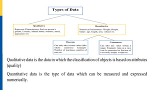
  • 8. Qualitative data is the data in which the classification of objects is based on attributes (quality) Quantitative data is the type of data which can be measured and expressed numerically.
  • 9. Understanding Data Columns are variables representing name, Gender, age, score, experience. Rows are representing observations. Now what type of data are these? First two columns represent Qualitative data and next three column represent Quantitative data.
  • 11. Examples for quantitative variables Size of shirt- 39, 40, 42, 50 etc. Per kilo prices of vegetables- Rs.30, Rs. 35, Rs.40 etc. Number of colleges in a city- 8, 12, 15 etc. Height of children- 1.2, 1.23, 1.32 etc. Examples for qualitative variables Names of cities – Kanpur, Delhi, Bangalore etc. Colours of hair- Black, White, Brown, Red etc. Taste of food – Sweet, Salty, neutral etc. Performance- Good, Excellent, bad etc. Data Set: A data set is a collection of observations on one or more variables.
  • 12. MEASUREMENT SCALES Measurement: The process of applying numbers to objects according to a set of rules. The four level of measurements are: nominal scale, ordinal scale, interval scale, and ratio scale. S. S. Stevens (1906 -1973) described the data into different scales of measurement as nominal, ordinal and cardinal data.
  • 13. Nominal Scale The nominal scale is a scale of measurement that is used for identification purposes. Sometimes known as categorical scale, These numbers have no real meaning and only act as labels. It helps in differentiating between objects. Example: For example, number representing on tea shirts of sports person. You could find one cricketer wearing number 12 and another wearing 85. They only help us to differentiate the person. The number provides no insight into the player’s position.
  • 15. Ordinal Scale Ordinal Scale involves the ranking or ordering of the observations. The items in this scale are classified according to the degree of occurrence of the variable. The attributes on an ordinal scale are usually arranged in ascending or descending order. It measures the degree of occurrence of the variable. Here, the order of variables is of prime importance and so is the labeling. Example: Class ranking :1st , 5th, 16th, 18th,25th,…. Teaching ability : good, average, bad. Grades of students: A, B, C, D. Social Status: High, middle, low
  • 16. Interval Scale In an Interval Scale numbers used to rank the objects also represents equal increments of the variable being measured. Examples: Time ,The difference between 6:00PM and 7:00PM is 1 hour, as is the difference between 4;00PM and 5:00PM. Celsius Temperature: The difference between 90 and 70 degrees is a 20 degrees, as is the difference between 40 and 60 degrees. Here increments are known, consistent and measurable. In Interval scale there is no 0 (zero). They do not have “true zero” there occurs arbitrary zero. There is no such thing as “no temperature”. “no time”
  • 17. Ratio Scale Ratio Scale is defined as a variable measurement scale that not only produces the order of variables but also makes the difference between variables known along with information on the value of true zero. It is calculated by assuming that the variables have an option for zero, the difference between the two variables is the same and there is a specific order between the options. The best examples of ratio scales are income, savings, weight, height etc. Note: Quantitative data is usually expressed using either Interval scale or Ratio Scale. Qualitative Data is expressed using either Nominal Scale or ordinal Scale.
  • 18. Methods of Data Collection Data means the raw facts and figures that have been collected. Data can be gathered by looking through existing sources, conducting experiments or by conducting surveys. Based on these sources of collections, statistical data may be classified as primary or secondary.
  • 19. PRIMARY DATA SECONDARY DATA Primary data are original observations collected by the investigator or his agent for the first time for any investigation using methods like surveys, interviews, or experiments. The secondary data is the collection of data from second hand information. This information is known as, given data is already collected from any one persons for some purpose, and it available for the present issues. And mostly these secondary data’s are not relevant and pure or original data. Example: Data collection from Government publications, websites, books, journal articles, internal records etc.
  • 20. Formation of Statistical series Individual series: The data as observed by an investigator is known as individual series. For example: Marks scored by 10 students: 100, 90, 72, 59, 40, 20, 23, 75, 61,43. Runs scored by the 11 players of the Indian cricket team in a match are given as follows: 25,65,03,12,35,46,67,56,00,31,17. Discrete Series: When the data collected are large in number and they are distinct then we can form a frequency distribution (the number of units associated with each value of the variable). The number of times a data occurs in a data set is known as the frequency of data. For example: In a quiz, the marks obtained by 20 students out of 30 are given as: 12,15,15,29,30,21,30,30,15,17,19,15,20,20,16,21,23,24,23,21
  • 21. Marks obtained in quiz Number of students(Frequency) 12 1 15 4 16 1 17 1 19 1 20 2 21 3 23 2 24 1 29 1 30 3 Total 20 Frequency Distribution Table (Ungrouped)
  • 22. Grouped series If the data are large in number, then the discrete series can be further reduced down by grouping them with the help of class intervals. Example: following table which represents the height of 200 students of high school. Grouped Frequency Distribution Table The first column of the table represents the class interval with a class width of 10. In each class, the lowest number denotes the lower class limit and the higher number indicates the upper-class limit. For the class 150-159, the lower class limit is 150 and the upper-class limit is 159. This is known as grouped frequency distribution. Height of Students (in cm.) Number of students(Frequency) 130-139 19 140-149 42 150-159 35 160-169 78 170-189 26 Total 200
  • 23. Continuous Series There are certain variables which will not have a distinct integer value. For example, weight, height, etc. In those cases the data will be of continuous type and grouping of those continuous data is known as “continuous series”. Example: Height in Centimeters of students: 155.0, 163.3, 155.0, 169.9, 163.9, 148.2, 151.5,128.9, 146.1, 145.2, 156.6, 159.9, 158.0, 153.4, 160.0, 149.3, 154.2, 164.7, 159.0,160.8, 157.1,176.0, 164.4, 170.0, 152.9, 169.3, 159.5,162.4, 173.6, 154.8,158.3,172.5,158.0, 154.0, 172.2, 148.0, 152.4,156.6, 157.7,165.3. In case of both grouped series and continuous series the class width depends on number of classes. To find the width of the classes we use the formula: i= 𝑳−𝑺 𝑲 where i is the class width, L is the largest value of the given data, S is the smallest value of the given data, K is the number of classes.
  • 24. i= 𝑳−𝑺 𝑲 = 172.5−145.2 5 =5.46 Now we round this approximate width to a convenient number, say 5. Heights Number of students 145-150 5 150-155 7 155-160 12 160-165 7 165-170 3 170-175 4 175-180 2
  • 25. Frequency Distribution or Frequency tables A systematic presentation of the values taken by a variable and the corresponding frequencies is called the frequency distribution of that variable. A tabular presentation of the frequency distribution is called the frequency table. Frequency distribution are of two types. (a) discrete frequency distribution (b) Continuous frequency distribution. A frequency distribution in which class intervals are considered is known as continuous frequency distribution. If class intervals are not considered it is a discrete frequency distribution.
  • 26. Frequency Distribution or Frequency tables(Contd.) The difference between the class limits of a class interval is known as the width of the class interval. In a frequency distribution, the class intervals may be inclusive or exclusive. If a class interval is such that the lower as well as the upper class limits are included in the same class interval it is inclusive class interval. If a class interval is such that the lower limit is included in the first class interval where as the upper class limit is included in the successive class interval it is exclusive class interval. This method is widely followed in practice. For example: 10,25,20, 12, 30, 46, 19, 15, 17, 20, 25. In inclusive class interval 20 will be included in 20-29 and in exclusive class interval 20 will be included in 20-30 instead of 10-20 interval. Inclusive Class interval Exclusive Class interval 10-19 5 10-20 5 20-29 4 20-30 4 30-39 1 30-40 1 40-49 1 40-50 1
  • 27. Example: Suppose a worker’s wages is Rs. 109.50. He is to be included in class I or the II? Under such circumstances, it is suggested that inclusive limits of classes be converted into exclusive limits. Correction factor= 1 2 110 − 109 =0.5 This is added to the upper limit and subtracted from the lower limit of the class. Wages in Rs: I method 100-109 110-119 120-129 130-139 140-149 150-159 Wages in Rs: II method 101-110 111-120 121-130 131-140 141-150 151-160 Wages in Rs: I method 99.5- 109.5 109.5- 119.5 119.5- 129.5 129.5- 139.5 139.5- 149.5 149.5- 159.5 Wages in Rs: II method 100.5- 110.5 110.5- 120.5 120.5- 130.5 130.5- 140.5 140.5- 150.5 150.5- 160.5
  • 28. Cumulative Frequency Distribution Cumulative frequency of a given variable or class represents the total frequency of all previous variables including the variable or the class. i.e the added –up frequencies are called Cumulative frequency Class Frequency Cumulative Frequency 10-14 6 6 15-19 11 17 20-24 12 29 25-29 10 39
  • 29. Example: The following data give the total number of iPods sold by a mail order company on each of 30 days. Construct a frequency distribution table. 8, 25, 11, 15, 29, 22, 10, 5, 17, 21, 22, 13, 26, 16, 18, 12, 9, 26, 20, 16, 23, 14, 19, 23, 20, 16, 27, 16, 21, 14
  • 30. Solution: In these data, the minimum value is 5, and the maximum value is 29. Suppose we decide to group these data using five classes of equal width. Then, Approximate width of each class = 29 – 5 / 5 = 4.8 Now we round this approximate width to a convenient number, say 5. The lower limit of the first class can be taken as 5 or any number less than 5. Frequency Distribution for the Data on iPods Sold i Pods Sold Frequency 5-9 /// 3 10-14 ///// / 6 15–19 ///// /// 8 20–24 ///// /// 8 25–29 ///// 5
  • 31. MEASURES OF CENTRAL TENDENCY  A Central tendency or average is a single value which represents the entire data.  Central tendency indicates where the center of the distribution tends to be. According to Croxton and Cowden ‘An average is a single value within the range of the data that is used to represent all the values in the series. Since an average is somewhere within range of data, it is sometimes called a measure of central value.
  • 32. PURPOSE AND FUNCTIONS OF CENTRAL TENDENCY  Brief Description of Data  Helpful in the Formulation of Policies  Basis of Statistical Analysis
  • 33. BRIEF DESCRIPTION OF DATA o Presents Simple and systematic description of the raw data. o Average reduces mass data into a single figure o One can draw the conclusions about the whole raw data with just a single figure.
  • 34. HELPFUL IN COMPARISON  Average help in making comparison of different sets of data.  For example, average income in XYZ state is much less than PQR State.  It can be concluded that XYZ state is a low income state in comparison to PQR State.
  • 35. HELPFUL IN FORMULATION OF POLICIES On the basis of average figure, Govt. of any country can formulate the policies For example, When Govt. of India finds the per capita income in India is very low, it can formulate suitable policies to improve the standard of people.
  • 36. BASIS OF STATISTICALANALYSIS  An Organization can make the statistical analysis on the basis of the average  For example, on the basis of sales of different model of a product, Organization decides which model need to produce in larger quantity.
  • 37. Types of Central Tendency
  • 38. Arithmetic Mean (A.M): The ‘Arithmetic Mean’ (referred to as ‘mean’) represented by 𝑋 is a most common measure of central tendency. The mean is a common measure in which all the values play an equal role. Arithmetic Mean (A.M) for Individual Series (raw data)
  • 39. Example1:The table below shows the number sales of five retail outlets in a day. The arithmetic mean of a set of data is defined as Mean = sum of the observations number of observations 𝑋 = 𝑋 𝑁 = 8+23+4+8+2 5 = 45 5 =9 ie, the average sales per retailer is Rs. 9000/-. Retailer 1 2 3 4 5 Sales (in 1000 Rs) 8 23 4 8 2
  • 40. Example 2:Hourly production of a manufacturing plant for eight hours is 1200, 1190,1210, 1180, 1190, 1220, 1230, 1180. Calculate the average production per hour. Solution: Average production per hour is 𝑋 = 1200+1190+1210+1180+1190+1220+1230+1180 8 𝑋 = 9600 8 =1200 hour. Example 3: Find the mean driving speed for 6 different cars on the same highway. 66 mph, 57 mph, 71 mph, 54 mph, 69 mph, 58 mph Solution: 66 + 57 + 71 + 54 + 69 + 58 6 = 375 6 = 62.5 mph.
  • 41. Example 4: If the arithmetic mean of 14 observations 26, 12, 14, 15, x, 17, 9, 11, 18, 16, 28, 20, 22, 8 is 17. Find the missing observation. Solution: Given 14 observations are: 26, 12, 14, 15, x, 17, 9, 11, 18, 16, 28, 20, 22, 8 Arithmetic mean = 17 We know that, Arithmetic mean = Sum of observations/Total number of observations 17 = (216 + x)/14 17 x 14 = 216 + x 216 + x = 238 x = 238 – 216 x = 22 Therefore, the missing observation is 22.
  • 42. Arithmetic mean for Discrete Series If the observations 𝑥1, 𝑥2, . . . 𝑥𝑁 have frequency f1,f2,f3,…..fN the arithmetic mean is given by
  • 43. Example: The students in a Statistics class were trying to study the heights of participants in a sports meet. They collected the height of 20 participants, as displayed in the table. Calculate the mean height of the participants. Height(in inches) 49 53 54 55 66 68 70 80 No of participants 1 2 4 5 3 2 2 1 Height (x) No of participants (f) fx 49 1 49 53 2 106 54 4 216 55 5 275 66 3 198 68 2 136 70 2 140 80 1 80 Total N=20 1200
  • 44. Example: A proof reads through 73 pages manuscript. The number of mistakes found on each of the pages are summarized in the table below. Determine the mean number of mistakes found per page. Mean number of mistakes is 4.09 No of mistakes 1 2 3 4 5 6 7 No of pages 5 9 12 17 14 10 6
  • 45. Example: Calculate the arithmetic mean from the following given data. X 4 6 8 10 12 14 frequency 5 9 11 8 4 3 X f Xf 4 5 20 6 9 54 8 11 88 10 8 80 12 4 48 14 3 42 Total N=40 Xf=332
  • 46. From the following data calculate arithmetic mean: No. of Calls (X): 0 1 2 3 4 5 6 7 Frequency (f): 14 21 25 43 51 40 39 12 X f fx 0 14 0 1 21 21 2 25 50 3 43 129 4 51 203 5 40 200 6 39 234 7 12 84 Total N=245 fx=922
  • 47. Example: From the following data for calculation of arithmetic mean, find the missing frequency. Given mean=31. X 10 20 30 40 50 60 f 8 12 20 10 ....... 4 X f fx 10 8 80 20 12 240 30 20 600 40 10 400 50 X 50X 60 4 240
  • 48. Find the missing frequency from the following distribution if its mean is 15.25 X 10 12 14 16 18 20 f 3 7 ? 20 8 5
  • 49. Arithmetic mean for Continuous Series Direct method 𝑋= fm 𝑁 m= mid value of various classes. f= frequency of each class N= total frequency.
  • 50. Example: From the following data, compute the arithmetic mean . Marks 0-10 10-20 20-30 30-40 40-50 50-60 60-70 70-80 No. Of students 5 10 25 30 20 10 5 5 Marks Mid- points(m) Number of students fm 0-10 5 5 25 10-20 15 10 150 20-30 25 25 625 30-40 35 30 1050 40-50 45 20 900 50-60 55 10 550 60-70 65 5 325 70-80 75 5 375 Total 110 4000
  • 51. Example: The table below show the age of 55 patients selected to study the effectiveness of a particular medicine. Calculate the mean age of the patients. Age 0-10 10-20 20-30 30-40 40-50 50-60 60-70 No. of Patients 5 7 17 12 5 2 7 Age Mid point (x) No of Patients (f) fx 0-10 5 5 25 10-20 15 7 105 20-30 25 17 425 30-40 35 12 420 40-50 45 5 225 50-60 55 2 110 60-70 65 7 455 Total N=55 1765
  • 52. Example: Calculate the arithmetic mean for the following data: Temperature (oC) -40- (-30) -30- (-20) -20-(-10) -10-0 0-10 10-20 20-30 No. of days 10 28 30 42 65 180 10 Temperature (oC) f m fm -40- (-30) 10 -35 -350 -30- (-20) 28 -25 -700 -20-(-10) 30 -15 -450 -10-0 42 -5 -210 0-10 65 5 325 10-20 180 15 2700 20-30 10 25 250 Total N=365 1565
  • 53. Example: The frequency distribution below represents the weights in kg of parcels carried by a small logistic company. Find the mean weight of parcels. Weight 10.0- 10.9 11.0- 11.9 12.0- 12.9 13.0- 13.9 14.0- 14.9 15.0- 15.9 16.0- 16.9 17.0- 17.9 18.0- 18.9 19.0- 19.9 No. of Parcels 2 3 5 8 12 15 13 11 6 2 Weight Mid point (x) No. of Parcels (f) fx 10.0-10.9 10.45 2 20.90 11.0-11.9 11.45 3 34.35 12.0-12.9 12.45 5 62.25 13.0-13.9 13.45 8 107.60 14.0-14.9 14.45 12 173.40 15.0-15.9 15.45 15 231.75 16.0-16.9 16.45 13 213.85 17.0-17.9 17.45 11 191.95 18.0-18.9 18.45 6 110.70 19.0-19.9 19.45 2 38.90
  • 54. Example: The following frequency distribution showing the marks obtained by 50 students in statistics at a certain college. Find the arithmetic mean. Marks 20-29 30-39 40-49 50-59 60-69 70-79 80-89 Frequency 1 5 12 15 9 6 2 Marks (x) f m fm 20-29 1 24.5 24.5 30-39 5 34.5 172.5 40-49 12 44.5 534.5 50-59 15 54.5 817.5 60-69 9 64.5 580.5 70-79 6 74.5 447.5 80-89 2 84.5 169.5 Total 50 2745
  • 55. Calculate the arithmetic mean from the following data. Price (in Rs) 15-18 18-21 21-24 24-27 27-30 30-33 33-36 Quantity Demanded 28 23 17 18 8 4 2 Price (in Rs) Mid-point (m) Frequency (f) f M 15-18 16.5 28 462 18-21 19.5 23 448.5 21-24 22.5 17 382.5 24-27 25.5 18 459 27-30 28.5 8 228 30-33 31.5 4 126 33-36 34.5 2 69 Total 100 2175
  • 56. The following distribution of persons according to different income groups. Find the average income of the persons. Income (in 1000) 0-8 8-16 16-24 24-32 32-40 40-48 No. of Persons 8 7 16 24 15 7 Class Mid-point (m) Frequency (f) f M 0-8 4 8 32 8-16 12 7 84 16-24 20 16 320 24-32 28 24 672 32-40 36 15 540 40-48 44 7 308 Total N=77 1956
  • 57. Find the mean form the following data: Marks Less than 10 Less than 20 Less than 30 Less than 40 Less than 50 Less than 60 Less than 70 Less than 80 No. of Students 5 20 45 70 80 88 98 100 Class Interval (Marks) Mid-Values (m) Students (f) fm 0 − 10 10 − 20 20 − 30 30 − 40 40 − 50 50 − 60 60 − 70 70 − 80 5 15 25 35 45 55 65 75 0-5=5 20-5=15 45-20=25 70-45=25 80-70=10 88-80=8 98-88=10 100-98=2 25 225 625 875 450 440 650 150 Σf=100 Σfm= 3440
  • 58. Example: Calculate arithmetic mean from the following data: Marks More than 0 More than 10 More than 20 More than 30 More than 40 More than 50 More than 60 More than 60 No. Of Students 150 140 100 80 80 70 30 14 Class Interval Mid- Values (m) No. of students (f) fm 0 − 10 10 − 20 20 − 30 30 − 40 40 − 50 50 − 60 60 − 70 70 − 80 5 15 25 35 45 55 65 75 150-140=10 140-100=40 100-80=20 80-80=0 80-70=10 70-30=40 30-14=16 14-0=14 50 600 500 0 450 2200 1040 1050 Σf=150 Σfm=5890
  • 59. The following table shows the age of workers in a factory. Find out the average age of workers. Calculation of mean in an inclusive series: Age (in Years) 20−29 30−39 40−49 50−59 60−69 Workers 10 8 6 4 2 Class Interval (Age) Mid-Values (m) Workers (f) fm 20 − 29 30 − 39 40 − 49 50 − 59 60 − 69 24.5 34.5 44.5 54.5 64.5 10 8 6 4 2 245 276 267 218 129 Σf=30 Σfm=1135
  • 60. Calculate the number of students against the class 30−40 of the following data, where mean is 28. Marks 0−10 10−20 20−30 30−40 40−50 50−60 Frequency 12 18 27 ? 17 6 Class Interval (Marks) Mid-Values (m) Frequency (f) fm 0 − 10 10 − 20 20 − 30 30 − 40 40 − 50 50 − 60 5 15 25 35 45 55 12 18 27 f 17 6 60 270 675 35f 765 330 Σf=80 + f Σfm=2100 + 35f
  • 61. Find the missing frequency form the following data, if athematic mean is 25.4. Class-interval 10−20 20−30 30−40 40−50 50−60 Frequency 20 15 10 ? 2 Class Interval Mid- Values (m) Frequency (f) fm 10 − 20 20 − 30 30 − 40 40 − 50 50 − 60 15 25 35 45 55 20 15 10 f 2 300 375 350 45f 110 Σf=47+f Σfm=1135 + 45 f
  • 62. Find the missing frequencies f1 and f2 in the table given below, it is being given that the mean of the given frequency distribution is 50. Class 0-20 20-40 40-60 60-80 80-100 Total Total Frequency 17 f1 32 f2 19 120 Class f m fm 0-20 17 10 170 20-40 f1 30 30 f1 40-60 32 50 1600 60-80 f 2 70 70 f 2 80-100 19 90 1710 Total N= 68+ f1+ f 2 3480+30f1+70 f 2
  • 63. The Average age of 20 students in a class is 16 years. One student whose age is 18 years has left the class. Find out average age of rest of the students. Given: Mean, 𝑋 = 16 years Number of observations, N= 20 𝑋 = 𝑋 𝑁 Total age of the 20 students = 𝑋 x N= 16 x20=320 Total age of the 19 students= 320-18=302 Thus, the average age of rest of the students is: 302 19 =15.89 years. Hence, the correct average age is 15.89 years.
  • 64. The average marks of 30 students in a class were 52. The top six students had an average of 31. What were the average marks of the other students? Given: N= 30, 𝑋 (30 students)=52 Average marks of top 6 students is 31 𝑋 = 𝑋 𝑁 X (Total marks of 30 students)=52 x30=1560 Total of 6 students marks 𝑋 =𝑋 xN= 31x6=186 ΣX of remaining 24 (30-6) students=1560-186=1374 Average marks of the other students = 1374 24 =57.25
  • 65. The mean of a group of 100 observations is known to be 50. Later it was discovered that two observations were misread as 92 and 8 instead of 192 and 88. Find the correct mean. Given that 𝑋 = 50 and n = 100. We have the sum of the observations, 𝑋 =𝑋 xN=100 x 50=5000 But it was wrong, because two observations 192 and 88 were misread as 92 and 8. So the corrected sum of observations is Corrected sum = 5000 - 92 -8 + 192 + 88 = 5180 So corrected mean; 𝑋 = Corrected Sum number of observations = 5180 100 =51.80
  • 66. The average marks scored by 10 students are 35 .Later the moderator awarded 2 grace marks to 4 students each and 1 grace mark to 2 students each. Find the average marks after moderation. Solution: Mean of 10 students =35 Mean = Sum of observations Total no of observations Sum = Mean x Total no of observations Sum= 350 After Moderation = 350+(4 x2)+(2 x1)=360 Average marks after moderation = 360 10 = 36.