


introducttion to Relational Databases ppt
- 1. CS4451 DATABASE MANAGEMENT SYSTEMS UNIT – I RELATIONAL DATABASES Introduction to databases - Purpose of Database System - Database system Applications - Views of data - Data Models - File system, Hierarchical and Network - Database system Architecture - Relational Model- keys - Relational Algebra. I. Introduction to databases DBMS contains information about a particular enterprise Collection of interrelated data Set of programs to access the data An environment that is both convenient and efficient to use
- 2. Database systems are used to manage collections of data that are: Highly valuable Relatively large Accessed by multiple users and applications, often at the same time. A modern database system is a complex software system whose task is to manage a large, complex collection of data. Databases touch all aspects of our lives Database Applications Examples Enterprise Information Sales: customers, products, purchases
- 3. Accounting: payments, receipts, assets Human Resources: Information about employees, salaries, payroll taxes. Manufacturing: management of production, inventory, orders, supply chain. Banking and finance customer information, accounts, loans, and banking transactions. Credit card transactions Finance: sales and purchases of financial instruments (e.g., stocks and bonds; storing real- time market data Universities: registration, grades Airlines: reservations, schedules
- 4. Telecommunication: records of calls, texts, and data usage, generating monthly bills, maintaining balances on prepaid calling cards Web-based services Online retailers: order tracking, customized recommendations Online advertisements Document databases Navigation systems: For maintaining the locations of varies places of interest along with the exact routes of roads, train systems, buses, etc.
- 5. So a database is a collection of related data that we can use for Defining - specifying types of data Constructing - storing & populating Manipulating - querying, updating, reporting Disadvantages Of File System Over Db In the early days, File-Processing system is used to store records. It uses various files for storing the records. Drawbacks of using file systems to store data: Data redundancy and inconsistency Multiple file formats, duplication of information in different files Difficulty in accessing data Need to write a new program to carry out each new task
- 6. Data isolation — multiple files and formats Integrity problems Hard to add new constraints or change existing ones Atomicity problem Failures may leave database in an inconsistent state with partial updates carried Out. E.g. transfer of funds from one account to another should either complete or not happen at all Concurrent access anomalies Concurrent accessed needed for performance Security problems Database systems offer solutions to all the above problems
- 7. II. PURPOSE OF DATABASE SYSTEM The typical file processing system is supported by a conventional operating system. The system stores permanent records in various files, and it needs different application programs to extract records from, and add records to, the appropriate files. A file processing system has a number of major disadvantages. Data redundancy and inconsistency Difficulty in accessing data Data isolation – multiple files and formats Integrity problems Atomicity of updates
- 8. Concurrent access by multiple users Security problems 1.Data redundancy and inconsistency: In file processing, every user group maintains its own files for handling its data processing applications. Example: Consider the UNIVERSITY database. Here, two groups of users might be the course registration personnel and the accounting office. The accounting office also keeps data on registration and related billing information, whereas the registration office keeps track of student courses and grades. Storing the same data multiple times is called data redundancy. This redundancy leads to several problems.
- 9. Need to perform a single logical update multiple times. Storage space is wasted. Files that represent the same data may become inconsistent. Data inconsistency is the various copies of the same data may no larger Agree. 2. Difficulty in accessing data File processing environments do not allow needed data to be retrieved in a convenient and efficient manner. 3. Data isolation Because data are scattered in various files, and files may be in different formats, writing new application programs to retrieve the appropriate data is difficult.
- 10. 4. Integrity problems The data values stored in the database must satisfy certain types of consistency constraints. Example: The balance of certain types of bank accounts may never fall below a prescribed amount.Developers enforce these constraints in the system by addition appropriate code in the various application programs 5. Atomicity problems Atomic means the transaction must happen in its entirety or not at all. It is difficult to ensure atomicity in a conventional file processing system. Example: Consider a program to transfer $50 from account A to account B. If a system failure occurs during the execution of the program, it is possible that the $50 was removed from account A but was not credited to account B, resulting in an inconsistent database state.
- 11. 6. Concurrent access anomalies For the sake of overall performance of the system and faster response, many systems allow multiple users to update the data simultaneously. In such an environment, interaction of concurrent updates is possible and may result in inconsistent data. To guard against this possibility, the system must maintain some form of supervision. But supervision is difficult to provide because data may be accessed by many different application programs that have not been coordinated previously. Example: When several reservation clerks try to assign a seat on an airline flight, the system should ensure that each seat can be accessed by only one clerk at a time for assignment to a passenger. 7. Security problems Enforcing security constraints to the file processing system is difficult.
- 12. III. APPLICATION OF DATABASE Database Applications Banking: all transactions Airlines: reservations, schedules Universities: registration, grades Sales: customers, products, purchases Manufacturing: production, inventory, orders, supply chain Human resources: employee records, salaries, tax deductions Telecommunication: Call History, Billing Credit card transactions: Purchase details, Statements
- 13. IV. VIEWS OF DATA It refers that how database is actually stored in database, what data and structure of data used by database for data. So describe all this database provides user with views and these are Data abstraction Instances and schema Data abstraction As a data in database are stored with very complex data structure so when user come and want to access any data, he will not be able to access data if he has go through this data structure. So to simplify the interaction of user and database, DBMS hides some information which is not of user interest, a this is called data abstraction:- So developer hides complexity from user and store abstract view of data.
- 14. Data abstraction has three level of abstractions Physical level / internal level Logical level / conceptual level view level / external level Physical level:- this is the lowest level of data abstraction which describe How data is actual stored in database. This level basically describe the data structure and access path /indexing use for accessing file. Logical level:- The next level of abstraction describe what data are stored in the database and what are the relationship existed among those of data. View level:- In this level user only interact with database and the complexity remain unview . user see data and there may be many views of one data like chart and graph.
- 15. V. DATA MODELS IN DBMS A Data Model is a logical structure of Database. It describes the design of database to reflect entities, attributes, relationship among data, constrains etc.
- 16. Types of Data Models: Object based logical Models – Describe data at the conceptual and view levels. 1. E-R Model An entity–relationship model (ER model) is a systematic way of describing and defining a business process. An ER model is typically implemented as a database. The main components of E-R model are: entity set and relationship set.
- 17. 2. Object oriented Model An object data model is a data model based on object-oriented programming, associating methods (procedures) with objects that can benefit from class hierarchies. Thus, ―objects are levels of abstraction that include attributes and behavior. Record based logical Models Like Object based model, they also describe data at the conceptual and view levels. These models specify logical structure of database with records, fields and attributes. 1. Relational Model In relational model, the data and relationships are represented by collection of inter-related tables. Each table is a group of column and rows, where column represents attribute of an entity and rows represents records.
- 18. Sample relationship Model: Student table with 3 columns and three records. 2. Hierarchical Model In hierarchical model, data is organized into a tree like structure with each record is having one parent record and many children. The main drawback of this model is that, it can have only one to many relationships between nodes. Sample Hierarchical Model Diagram
- 19. 3. Network Model Network Model is same as hierarchical model except that it has graph-like structure rather than a tree- based structure. Unlike hierarchical model, this model allows each record to have more than one parent record. Physical Data Models – These models describe data at the lowest level of abstraction. Three Schema Architecture The goal of the three schema architecture is to separate the user applications and the physical database. The schemas can be defined at the following levels: 1. The internal level It has an internal schema which describes the physical storage structure of the database. Uses a physical data model and describes the complete details of data storage and access paths for the database.
- 20. 2. The conceptual level It has a conceptual schema which describes the structure of the database for users. It hides the details of the physical storage structures, and concentrates on describing entities, data types, relationships, user operations and constraints. Usually a representational data model is used to describe the conceptual schema. 3. The External or View level It includes external schemas or user vies. Each external schema describes the part of the database that a particular user group is interested in and hides the rest of the database from that user group. Represented using the representational data model
- 21. The three schema architecture is used to visualize the schema levels in a database. The three schemas are only descriptions of data, the data only actually exists is at the physical level
- 22. VI. File System File based systems were an early attempt to computerize the manual system. It is also called a traditional based approach in which a decentralized approach was taken where each department stored and controlled its own data with the help of a data processing specialist. The main role of a data processing specialist was to create the necessary computer file structures, and also manage the data within structures and design some application programs that create reports based on file data.
- 23. In the above figure: Consider an example of a student's file system. The student file will contain information regarding the student (i.e. roll no, student name, course etc.). Similarly, we have a subject file that contains information about the subject and the result file which contains the information regarding the result. Some fields are duplicated in more than one file, which leads to data redundancy. So to overcome this problem, we need to create a centralized system, i.e. DBMS approach.
- 24. DBMS: A database approach is a well-organized collection of data that are related in a meaningful way which can be accessed by different users but stored only once in a system. The various operations performed by the DBMS system are: Insertion, deletion, selection, sorting etc. In the above figure, In the above figure, duplication of data is reduced due to centralization of data.
- 26. VII. Hierarchical and Network 1. Hierarchical Data Model: Hierarchical data model is the oldest type of the data model. It was developed by IBM in 1968. It organizes data in the tree-like structure. Hierarchical model consists of the following : It contains nodes which are connected by branches. The topmost node is called the root node. If there are multiple nodes appear at the top level, then these can be called as root segments. Each node has exactly one parent. One parent may have many child.
- 27. In the above figure, Electronics is the root node which has two children i.e. Televisions and Portable Electronics. These two has further children for which they act as parent. For example: Television has children as Tube, LCD and Plasma, for these three Television act as parent. It follows one to many relationship.
- 28. 2. Network Data Model: It is the advance version of the hierarchical data model. To organize data it uses directed graphs instead of the tree-structure. In this child can have more than one parent. It uses the concept of the two data structures i.e. Records and Sets. In the above figure, Project is the root node which has two children i.e. Project 1 and Project 2. Project 1 has 3 children and Project 2 has 2 children. Total there are 5 children i.e Department A, Department B and Department C, they are network related children as we said that this model can have more than one parent. So, for the Department B and Department C have two parents i.e. Project 1 and Project 2.
- 29. F
- 30. C
- 31. VIII. Database system Architecture A Database stores a lot of critical information to access data quickly and securely. Hence it is important to select the correct architecture for efficient data management. DBMS Architecture helps users to get their requests done while connecting to the database. We choose database architecture depending on several factors like the size of the database, number of users, and relationships between the users. There are two types of database models that we generally use, logical model and physical model. Several types of architecture are there in the database which we will deal with in the next section.
- 32. Types of DBMS Architecture There are several types of DBMS Architecture that we use according to the usage requirements. Types of DBMS Architecture are discussed here. 1-Tier Architecture 2-Tier Architecture 3-Tier Architecture 1-Tier Architecture In 1-Tier Architecture the database is directly available to the user, the user can directly sit on the DBMS and use it that is, the client, server, and Database are all present on the same machine. For Example: to learn SQL we set up an SQL server and the database on the local system.
- 33. Advantages of 1-Tier Architecture Simple Architecture: 1-Tier Architecture is the most simple architecture to set up, as only a single machine is required to maintain it. Cost-Effective: No additional hardware is required for implementing 1-Tier Architecture, which makes it cost-effective. Easy to Implement: 1-Tier Architecture can be easily deployed, and hence it is mostly used in small projects.
- 34. 2-Tier Architecture The 2-tier architecture is similar to a basic client-server model. The application at the client end directly communicates with the database on the server side. APIs like ODBC and JDBC are used for this interaction. The server side is responsible for providing query processing and transaction management functionalities. On the client side, the user interfaces and application programs are run. The application on the client side establishes a connection with the server side to communicate with the DBMS.
- 35. An advantage of this type is that maintenance and understanding are easier, and compatible with existing systems. However, this model gives poor performance when there are a large number of users. Advantages of 2-Tier Architecture Easy to Access: 2-Tier Architecture makes easy access to the database, which makes fast retrieval. Scalable: We can scale the database easily, by adding clients or upgrading hardware. Low Cost: 2-Tier Architecture is cheaper than 3-Tier Architecture and Multi-Tier Architecture. Easy Deployment: 2-Tier Architecture is easier to deploy than 3-Tier Architecture. Simple: 2-Tier Architecture is easily understandable as well as simple because of only two components.
- 36. 3-Tier Architecture In 3-Tier Architecture, there is another layer between the client and the server. The client does not directly communicate with the server. Instead, it interacts with an application server which further communicates with the database system and then the query processing and transaction management takes place. This intermediate layer acts as a medium for the exchange of partially processed data between the server and the client. This type of architecture is used in the case of large web applications.
- 37. Advantages of 3-Tier Architecture Enhanced scalability: Scalability is enhanced due to the distributed deployment of application servers. Now, individual connections need not be made between the client and server. Data Integrity: 3-Tier Architecture maintains Data Integrity. Since there is a middle layer between the client and the server, data corruption can be avoided/removed. Security: 3-Tier Architecture Improves Security. This type of model prevents direct interaction of the client with the server thereby reducing access to unauthorized data.
- 38. IX. Relational Model Structure of Relational Databases A relational database consists of a collection of tables, each of which is assigned a unique name. For example, consider the instructor table of below figure, which stores information about instructors. The table has four column headers: ID, name, dept name, and salary. Each row of this table records information about an instructor, consisting of the instructor’s ID, name, dept name, and salary.
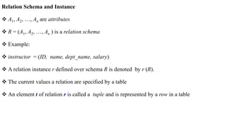
- 40. Relation Schema and Instance A1, A2, …, An are attributes R = (A1, A2, …, An ) is a relation schema Example: instructor = (ID, name, dept_name, salary) A relation instance r defined over schema R is denoted by r (R). The current values a relation are specified by a table An element t of relation r is called a tuple and is represented by a row in a table
- 41. Attributes The set of allowed values for each attribute is called the domain of the attribute. Attribute values are (normally) required to be atomic; that is, indivisible. The special value null is a member of every domain. Indicated that the value is “unknown”. The null value causes complications in the definition of many operations. Relations are Unordered Order of tuples is irrelevant (tuples may be stored in an arbitrary order) Example: instructor relation with unordered tuples
- 42. Database Schema Database schema -- is the logical structure of the database. Database instance -- is a snapshot of the data in the database at a given instant in time.
- 43. X. Keys Keys play an important role in the relational database. It is used to uniquely identify any record or row of data from the table. It is also used to establish and identify relationships between tables. For example, ID is used as a key in the Student table because it is unique for each student. In the PERSON table, passport_number, license_number, SSN are keys since they are unique for each person.
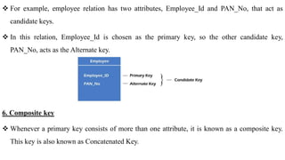
- 44. Types of keys: 1. Primary key It is the first key used to identify one and only one instance of an entity uniquely. An entity can contain multiple keys, as we saw in the PERSON table. The key which is most suitable from those lists becomes a primary key. In the EMPLOYEE table, ID can be the primary key since it is unique for each employee.
- 45. In the EMPLOYEE table, we can even select License_Number and Passport_Number as primary keys since they are also unique. For each entity, the primary key selection is based on requirements and developers. 2. Candidate key A candidate key is an attribute or set of attributes that can uniquely identify a tuple. Except for the primary key, the remaining attributes are considered a candidate key. The candidate keys are as strong as the primary key.
- 46. For example: In the EMPLOYEE table, id is best suited for the primary key. The rest of the attributes, like SSN, Passport_Number, License_Number, etc., are considered a candidate key. 3. Super Key Super key is an attribute set that can uniquely identify a tuple. A super key is a superset of a candidate key.
- 47. For example: In the above EMPLOYEE table, for(EMPLOEE_ID, EMPLOYEE_NAME), the name of two employees can be the same, but their EMPLYEE_ID can't be the same. Hence, this combination can also be a key. The super key would be EMPLOYEE-ID (EMPLOYEE_ID, EMPLOYEE-NAME), etc.
- 48. 4. Foreign key Foreign keys are the column of the table used to point to the primary key of another table. Every employee works in a specific department in a company, and employee and department are two different entities. So we can't store the department's information in the employee table. That's why we link these two tables through the primary key of one table. We add the primary key of the DEPARTMENT table, Department_Id, as a new attribute in the EMPLOYEE table. In the EMPLOYEE table, Department_Id is the foreign key, and both the tables are related.
- 49. 5. Alternate key There may be one or more attributes or a combination of attributes that uniquely identify each tuple in a relation. These attributes or combinations of the attributes are called the candidate keys. One key is chosen as the primary key from these candidate keys, and the remaining candidate key, if it exists, is termed the alternate key. In other words, the total number of the alternate keys is the total number of candidate keys minus the primary key. The alternate key may or may not exist. If there is only one candidate key in a relation, it does not have an alternate key.
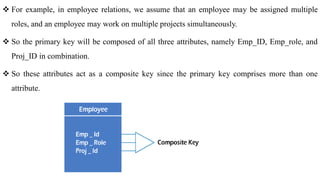
- 50. For example, employee relation has two attributes, Employee_Id and PAN_No, that act as candidate keys. In this relation, Employee_Id is chosen as the primary key, so the other candidate key, PAN_No, acts as the Alternate key. 6. Composite key Whenever a primary key consists of more than one attribute, it is known as a composite key. This key is also known as Concatenated Key.
- 51. For example, in employee relations, we assume that an employee may be assigned multiple roles, and an employee may work on multiple projects simultaneously. So the primary key will be composed of all three attributes, namely Emp_ID, Emp_role, and Proj_ID in combination. So these attributes act as a composite key since the primary key comprises more than one attribute.
- 52. 7. Artificial key The key created using arbitrarily assigned data are known as artificial keys. These keys are created when a primary key is large and complex and has no relationship with many other relations. The data values of the artificial keys are usually numbered in a serial order.
- 53. XI. Relational Algebra The relational algebra consists of a set of operations that take one or two relations as input and produce a new relation as their result. Some of these operations, such as the select, project, and rename operations, are called unary operations because they operate on one relation. The other operations, such as union, Cartesian product, and set difference, operate on pairs of relations and are, therefore, called binary operations.
- 54. Six basic operators 1. select: 2. project: 3. union: 4. set difference: – 5. Cartesian product: x 6. rename: 1. Select Operation The select operation selects tuples that satisfy a given predicate. Notation: p (r) p is called the selection predicate
- 55. Example: select those tuples of the instructor relation where the instructor is in the “Physics” department. Query : dept_name=“Physics” (instructor) Result Instructor table
- 56. We allow comparisons using in the selection predicate. =, , >, . <. We can combine several predicates into a larger predicate by using the connectives: (and), (or), (not) Example: Find the instructors in Physics with a salary greater $90,000, we write: dept_name=“Physics” salary > 90,000 (instructor) The select predicate may include comparisons between two attributes. Example, find all departments whose name is the same as their building name: dept_name=building (department)
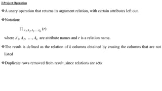
- 57. 2.Project Operation A unary operation that returns its argument relation, with certain attributes left out. Notation: A1,A2,A3 ….Ak (r) where A1, A2, …, Ak are attribute names and r is a relation name. The result is defined as the relation of k columns obtained by erasing the columns that are not listed Duplicate rows removed from result, since relations are sets
- 58. Project Operation Example • Example: eliminate the dept_name attribute of instructor • Query: ID, name, salary (instructor) • Result:
- 59. Composition of Relational Operations The result of a relational-algebra operation is relation and therefore of relational-algebra operations can be composed together into a relational-algebra expression. Consider the query -- Find the names of all instructors in the Physics department. name( dept_name =“Physics” (instructor)) Instead of giving the name of a relation as the argument of the projection operation, we give an expression that evaluates to a relation.
- 60. Cartesian-Product Operation The Cartesian-product operation (denoted by X) allows us to combine information from any two relations. Example: the Cartesian product of the relations instructor and teaches is written as: instructor X teaches We construct a tuple of the result out of each possible pair of tuples: one from the instructor relation and one from the teaches relation Since the instructor ID appears in both relations we distinguish between these attribute by attaching to the attribute the name of the relation from which the attribute originally came. instructor.ID teaches.ID
- 61. The instructor X teaches table
- 62. Join Operation The Cartesian-Product associates every tuple of instructor with every tuple of teaches. instructor X teaches Most of the resulting rows have information about instructors who did NOT teach a particular course. To get only those tuples of “instructor X teaches “ that pertain to instructors and the courses that they taught, we write: instructor.id = teaches.id (instructor x teaches )) We get only those tuples of “instructor X teaches” that pertain to instructors and the courses that they taught.
- 63. The table corresponding to: instructor.id = teaches.id (instructor x teaches))
- 64. The join operation allows us to combine a select operation and a Cartesian-Product operation into a single operation. Consider relations r (R) and s (S) Let “theta” be a predicate on attributes in the schema R “union” S. The join operation r ⋈𝜃 s is defined as follows: 𝑟 ⋈𝜃 𝑠 = 𝜎𝜃 (𝑟 × 𝑠) Thus instructor.id = teaches.id (instructor x teaches )) Can equivalently be written as instructor ⋈ Instructor.id = teaches.id teaches.
- 65. Union Operation The union operation allows us to combine two relations Notation: r s For r s to be valid. 1. r, s must have the same arity (same number of attributes) 2. The attribute domains must be compatible (example: 2nd column of r deals with the same type of values as does the 2nd column of s) Example: to find all courses taught in the Fall 2017 semester, or in the Spring 2018 semester, or in both course_id ( semester=“Fall” Λ year=2017 (section)) course_id ( semester=“Spring” Λ year=2018 (section))
- 66. Result of: course_id ( semester=“Fall” Λ year=2017 (section)) course_id ( semester=“Spring” Λ year=2018 (section)) Set-Intersection Operation The set-intersection operation allows us to find tuples that are in both the input relations. Notation: r s Assume: Result r, s have the same arity attributes of r and s are compatible
- 67. Example: Find the set of all courses taught in both the Fall 2017 and the Spring 2018 semesters. course_id ( semester=“Fall” Λ year=2017 (section)) course_id ( semester=“Spring” Λ year=2018 (section)) Result Set Difference Operation The set-difference operation allows us to find tuples that are in one relation but are not in another. Notation r – s Set differences must be taken between compatible relations. r and s must have the same arity attribute domains of r and s must be compatible
- 68. • Example: to find all courses taught in the Fall 2017 semester, but not in the Spring 2018 semester course_id ( semester=“Fall” Λ year=2017 (section)) − course_id ( semester=“Spring” Λ year=2018 (section)) The Assignment Operation It is convenient at times to write a relational-algebra expression by assigning parts of it to temporary relation variables. The assignment operation is denoted by and works like assignment in a programming language. Example:Find all instructor in the “Physics” and Music department. Physics dept_name=“Physics” (instructor) Music dept_name=“Music” (instructor) Physics Music
- 69. With the assignment operation, a query can be written as a sequential program consisting of a series of assignments followed by an expression whose value is displayed as the result of the query. The Rename Operation The results of relational-algebra expressions do not have a name that we can use to refer to them. The rename operator, , is provided for that purpose The expression: returns the result of expression E under the name x x (E) Another form of the rename operation: x(A1,A2, .. An) (E)
- 70. Equivalent Queries There is more than one way to write a query in relational algebra. Example: Find information about courses taught by instructors in the Physics department with salary greater than 90,000 Query 1 dept_name=“Physics” salary > 90,000 (instructor) Query 2 dept_name=“Physics” ( salary > 90.000 (instructor)) The two queries are not identical; they are, however, equivalent -- they give the same result on any database.
- 71. Equivalent Queries There is more than one way to write a query in relational algebra. Example: Find information about courses taught by instructors in the Physics department Query 1 dept_name=“Physics” (instructor ⋈ instructor.ID = teaches.ID teaches) Query 2 (dept_name=“Physics” (instructor)) ⋈ instructor.ID = teaches.ID teaches The two queries are not identical; they are, however, equivalent -- they give the same result on any database.