1. A GUEST LECTURE
on
COMPUTER NETWORKS
for
III YEAR B.TECH(CSE) – I SEM
BY
DR. K. KRANTHI KUMAR
Associate Professor, Dept of IT,
Sreenidhi Institute of science and technology, Hyderabad,
[email protected], 9848624931
JAWAHARLAL NEHRU TECHNOLOGICAL UNIVERSITY HYDERABAD
UNIVERSITY COLLEGE OF ENGINEERING RAJANNA SIRCILLA
Agraharam, Rajanna Sircilla District, Telangana State, India. Pin Code: 505302
2. COMPUTER NETWORKS SYLLABUS
UNIT - I
Network hardware, Network software, OSI, TCP/IP Reference models, Example
Networks: ARPANET, Internet. Physical Layer: Guided Transmission media:
twisted pairs, coaxial cable, fiber optics, Wireless Transmission. Data link layer:
Design issues, framing, Error detection and correction.
UNIT - II
Elementary data link protocols: simplex protocol, A simplex stop and wait protocol
for an error-free channel, A simplex stop and wait protocol for noisy channel.
Sliding Window protocols: A one-bit sliding window protocol, A protocol using Go-
Back-N, A protocol using Selective Repeat, Example data link protocols.
Medium Access sub layer: The channel allocation problem, Multiple access
protocols: ALOHA, Carrier sense multiple access protocols, collision free
protocols. Wireless LANs, Data link layer switching.
3. UNIT - III
Network Layer: Design issues, Routing algorithms: shortest path routing,
Flooding, Hierarchical routing, Broadcast, Multicast, distance vector
routing, Congestion Control Algorithms, Quality of Service,
Internetworking, The Network layer in the internet.
UNIT - IV
Transport Layer: Transport Services, Elements of Transport protocols,
Connection management, TCP and UDP protocols.
UNIT - V
Application Layer –Domain name system, SNMP, Electronic Mail; the
World WEB, HTTP, Streaming audio and video.
TEXT BOOK:
1. Computer Networks -- Andrew S Tanenbaum, David. j. Wetherall, 5th
Edition. Pearson Education/PHI .
4. Sliding window protocols
Must be able to transmit data in both directions.
Choices for utilization of the reverse channel:
mix DATA frames with ACK frames.
Piggyback the ACK
Receiver waits for DATA traffic in the opposite direction.
Use the ACK field in the frame header to send sequence
number of frame being ACKed.
better use of the channel capacity.
5. Sliding window protocols:
In the Previous protocols ,Data frames were transmitted in
one direction only.
In most practical situations ,there is a need for transmitting
data in both directions.
One way of achieving full-duplex data transmission is to have
two separate communication channels and each one for
simplex data traffic (in different directions)
we have two separate physical circuits ,each with a “forward”
channel (for data) and a “reverse” channel( for
acknowledgements).
source Destination
Data
Acknowledgement
s
6. Sliding window protocols:
Disadvantage: The bandwidth of the reverse channel is
almost entirely wasted.
A better idea is to use the same circuits for data in both
directions
In this model the data frames from A and B are
intermixed with the acknowledgement frames from A to
B.
Kind: kind field in the header of an incoming frame, the
receiver can tell whether the frame is data or
acknowledgements.
7. Sliding window protocols:
Piggybacking:
source Destination
Frame sent(Frame1)
Ack(frame1)+Frame
2
• When a data frame arrives, instead of immediately sending a
separate control frame, the receiver restrains itself and waits until
the network layer passes it the next packet.
• The acknowledgement is attached to the outgoing data frame
• Disadv: This technique is temporarily delaying outgoing
acknowledgements.
• If the datalinklayer waits longer than the senders timeout period,
the frame will be retransmitted.
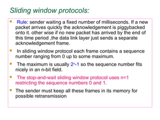
8. Sliding window protocols:
Rule: sender waiting a fixed number of milliseconds. If a new
packet arrives quickly the acknowledgement is piggybacked
onto it. other wise if no new packet has arrived by the end of
this time period ,the data link layer just sends a separate
acknowledgement frame.
In sliding window protocol each frame contains a sequence
number ranging from 0 up to some maximum.
The maximum is usually 2n
-1 so the sequence number fits
nicely in an n-bit field.
The stop-and-wait sliding window protocol uses n=1
restricting the sequence numbers 0 and 1.
The sender must keep all these frames in its memory for
possible retransmission
9. Sliding window protocols:
Thus if the maximum window size is n, the sender needs
n buffers to hold the unacknowledged frames
3 bit field -000
001
010..etc
here n=3 i.e. 23
-1=7
window size is 0 to 7
Sliding window :: sender has a window of frames and
maintains a list of consecutive sequence numbers for
frames that it is permitted to send without waiting for
ACKs.
receiver has a window that is a list of frame sequence
numbers it is permitted to accept.
Note – sending and receiving windows do NOT have to be
the same size.
10. Sliding window protocols:
A sliding window of size 1, with a 3-bit sequence number.
(a) Initially.
(b) After the first frame has been sent.
(c) After the first frame has been received.
(d) After the first acknowledgement has been received.
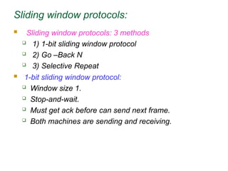
11. Sliding window protocols:
Sliding window protocols: 3 methods
1) 1-bit sliding window protocol
2) Go –Back N
3) Selective Repeat
1-bit sliding window protocol:
Window size 1.
Stop-and-wait.
Must get ack before can send next frame.
Both machines are sending and receiving.
12. 1-bit sliding protocol :
Example:
A trying to send its frame 0 to B.
B trying to send its frame 0 to A.
Imagine A's timeout is too short. A repeatedly times out and
sends multiple copies to B, all with seq=0, ack=1.
When first one of these gets to B, it is accepted. Set
expected=1. B sends its frame, seq=0, ack=0.
All subsequent copies of A's frame rejected since seq=0
not equal to expected. All these also have ack=1.
B repeatedly sends its frame, seq=0, ack=0. But A not
getting it because it is timing out too soon.
Eventually, A gets one of these frames. A has its ack now
(and B's frame). A sends next frame and acks B's frame.
13. 1-bit sliding protocol :
Two scenarios for protocol 4. (a) Normal case. (b) Abnormal case. The
notation is (seq, ack, packet number). An asterisk indicates where a
network layer accepts a packet.
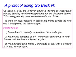
14. A protocol using Go Back N:
Go Back n, is for the receiver simply to discard all subsequent
frames, sending no acknowledgements for the discarded frames.
This strategy corresponds to a receive window of size 1.
The data link layer refuses to accept any frame except the next
one it must give to the network layer.
Points: fig ( a)
1) frame 0 and 1 correctly received and Acknowledged
2) Frame 2 is damaged or lost ,The sender continuous to send
frames until the timer for frame 2 expires.
3) Then it backs up to frame 2 and starts all over with it ,sending
2,3,4 etc. all over again.
16. Go-Back-N ARQ
• Pipelining improves the efficiency of the transmission
• In the Go-Back-N Protocol, the sequence numbers are modulo 2m
, where m is the size of
the sequence number field in bits
• The send window is an abstract concept defining an imaginary box of size 2m
− 1 with
three variables: Sf, Sn, and Ssize
• The send window can slide one or more slots when a valid acknowledgment arrives.
17. Go-Back-N ARQ
• Receive window for Go-Back-N ARQ
• The receive window is an abstract concept defining an
imaginary box of size 1 with one single variable Rn. The window
slides when a correct frame has arrived; sliding occurs one slot
at a time.
19. Go-Back-N ARQ: Send Window Size
• In Go-Back-N ARQ, the size of the send window must be less than
2m
; the size of the receiver window is always 1
• Stop-and-Wait ARQ is a special case of Go-Back-N ARQ in which the
size of the send window is 1
22. Selective Repeat:
When selective repeat is used ,a bad frame that is received is
discarded. But good frames after it are buffered.
when the senders timeout ,only the oldest unacknowledged
frame is retransmitted.
If that frames arrives correctly ,the receiver can deliver it to the
network layer in sequence all the frames it has buffered.
fig (b) :
1) Frames 0 and 1 correctly received and acknowledged.
2) Frame 2 is lost, when frame 3 arrives at the receiver ,the
data link layer notices that it has a missed frame. so it sends
back a NAK for 2 but buffers 3
3) when frame 4 and 5 arrive ,they are buffered by the data
link layer instead of being passed to the network layer
4)The NAK 2 gets back to the sender which immediately
resends frame 2.
28. Piggybacking
• To improve the efficiency of the bidirectional protocols
• Piggybacking in Go-Back-N ARQ
29. CSMA: Carrier Sense Multiple Access
Protocols in which stations listen for a carrier (i.e.,
transmission) and act accordingly are called carrier sense
protocols.
Adv:
To minimize the chance of collision
Increases the performance.
CSMA principle is “sense before transmit” or “listen
before talk”.
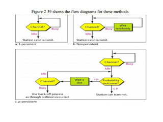
30. CSMA Methods
1. 1-persistent CSMA- constant length packets.
2. non-persistent CSMA- to sense the channel.
3. p-persistent CSMA
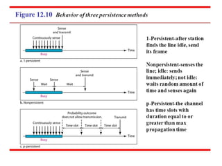
32. 1-persistent
When a station has data to send, it first listens to channel to see if
any one else is transmitting at that moment.
If the channel is busy, the station continuously senses the channel
until it becomes idle.
When the station detects an idle channel, it transmits a frame.
If a collision occurs, the station waits a random amount of time
and starts all over again.
The station transmits with a probability of 1 whenever if finds the
channel idle.
This method has highest chance of collision because two or more
stations may find the line idle and send their frames immediately.
33. Non-persistent CSMA
A station that has a frame to send it senses the line.
If the line is idle, it sends immediately.
If the line is not idle, it waits a random amount of time and then
senses the line again.
This approach reduces the chance of collision because it is
unlikely that two or more stations will wait the same amount of
time and retry to send simultaneously.
This algorithm should lead to better channel utilization and
longer delays than 1-persistant CSMA.
34. P-persistent CSMA
This method is used if the channel has time slots with a slot
duration equal to or greater than the maximum propagation
time.
It combines advantages of the other two strategies.
It reduces the chance of collision and improves efficiency.
35. P-persistent CSMA
In this method, after station finds the line idle it follows these
steps:
1.With probability ‘p’, the station sends its frame.
2.With probability q=1-p, the station waits for the beginning of the
next time slot and checks the line again.
a. If the line is idle, it goes to step 1.
b. If the line is busy, it acts as though a collision has occurred
and uses the back-off procedure(which discussed earlier).
37. Carrier Sense Multiple Access with
Collision Detection(CSMA/CD)
• In this method, a station monitors the medium after it sends a
frame to see if the transmission was successful. If so, the
station is finished. If, however, there is a collision, the frame
is sent again.
40. Minimum Frame Size
• For CSMA/CD to work, we need restriction on the frame size.
• Therefore, the frame transmission time Tfr must be at least
two times the maximum propagation time Tp.
• To understand the reason, let us think about worst-case
scenario. If two stations involved in a collision are the
maximum distance apart, the signal from the first takes Tp to
reach the second, and the effect of the collision takes another
Tp to reach the first.
• So the requirement is that the first station must still be
transmitting after 2Tp
42. IEEE Standards
• In 1985, the Computer Society of the IEEE started a project, called
Project 802, to set standards to enable intercommunication among
equipment from a variety of manufacturers. Project 802 is a way of
specifying functions of the physical layer and the data link layer of
major LAN protocols.
43. IEEE 802 Working Group
Active working groups Inactive or disbanded working groups
802.1 Higher Layer LAN Protocols Working
Group
802.3 Ethernet Working Group
802.11 Wireless LAN Working Group
802.15 Wireless Personal Area Network
(WPAN) Working Group
802.16 Broadband Wireless Access Working
Group
802.17 Resilient Packet Ring Working Group
802.18 Radio Regulatory TAG
802.19 Coexistence TAG
802.20 Mobile Broadband Wireless Access
(MBWA) Working Group
802.21 Media Independent Handoff Working
Group
802.22 Wireless Regional Area Networks
802.2 Logical Link Control Working Group
802.4 Token Bus Working Group
802.5 Token Ring Working Group
802.7 Broadband Area Network Working
Group
802.8 Fiber Optic TAG
802.9 Integrated Service LAN Working
Group
802.10 Security Working Group
802.12 Demand Priority Working Group
802.14 Cable Modem Working Group
45. Wireless Local Area Networks
• The proliferation of laptop computers and
other mobile devices (PDAs and cell phones)
created an obvious application level demand
for wireless local area networking.
• Companies jumped in, quickly developing
incompatible wireless products in the 1990’s.
• Industry decided to entrust standardization to
IEEE committee that dealt with wired LANS –
namely, the IEEE 802 committee!!
46. IEEE 802 Standards Working Groups
Figure 1-38. The important ones are marked with *. The ones marked with
are hibernating. The one marked with † gave up.
47. Categories of Wireless Networks
• Base Station :: all communication through an access
point {note hub topology}. Other nodes can be fixed or
mobile.
• Infrastructure Wireless :: base station network is
connected to the wired Internet.
• Ad hoc Wireless :: wireless nodes communicate directly
with one another.
• MANETs (Mobile Ad Hoc Networks) :: ad hoc nodes are
mobile.
50. Wireless Physical Layer
• Physical layer conforms to OSI (five options)
– 1997: 802.11 infrared, FHSS, DHSS
– 1999: 802.11a OFDM and 802.11b HR-DSSS
– 2001: 802.11g OFDM
• 802.11 Infrared
– Two capacities 1 Mbps or 2 Mbps.
– Range is 10 to 20 meters and cannot penetrate walls.
– Does not work outdoors.
• 802.11 FHSS (Frequence Hopping Spread Spectrum)
– The main issue is multipath fading.
– 79 non-overlapping channels, each 1 Mhz wide at low end of 2.4
GHz ISM band.
– Same pseudo-random number generator used by all stations.
– Dwell time: min. time on channel before hopping (400msec).
51. Wireless Physical Layer
• 802.11 DSSS (Direct Sequence Spread Spectrum)
– Spreads signal over entire spectrum using pseudo-random
sequence (similar to CDMA see Tanenbaum sec. 2.6.2).
– Each bit transmitted using an 11 chips Barker sequence, PSK at
1Mbaud.
– 1 or 2 Mbps.
• 802.11a OFDM (Orthogonal Frequency Divisional Multiplexing)
– Compatible with European HiperLan2.
– 54Mbps in wider 5.5 GHz band transmission range is limited.
– Uses 52 FDM channels (48 for data; 4 for synchronization).
– Encoding is complex ( PSM up to 18 Mbps and QAM above this
capacity).
– E.g., at 54Mbps 216 data bits encoded into into 288-bit symbols.
– More difficulty penetrating walls.
52. Wireless Physical Layer
• 802.11b HR-DSSS (High Rate Direct Sequence Spread
Spectrum)
– 11a and 11b shows a split in the standards committee.
– 11b approved and hit the market before 11a.
– Up to 11 Mbps in 2.4 GHz band using 11 million chips/sec.
– Note in this bandwidth all these protocols have to deal
with interference from microwave ovens, cordless phones
and garage door openers.
– Range is 7 times greater than 11a.
53. Wireless Physical Layer
• 802.11g OFDM(Orthogonal Frequency Division
Multiplexing)
– An attempt to combine the best of both 802.11a and
802.11b.
– Supports bandwidths up to 54 MBps.
– Uses 2.4 GHz frequency for greater range.
– Is backward compatible with 802.11b.
54. 802.11 MAC Sublayer Protocol
• In 802.11 wireless LANs, “seizing channel” does not
exist as in 802.3 wired Ethernet.
• Two additional problems:
– Hidden Terminal Problem
– Exposed Station Problem
• To deal with these two problems 802.11 supports
two modes of operation DCF (Distributed
Coordination Function) and PCF (Point Coordination
Function).
• All implementations must support DCF, but PCF is
optional.
56. The Hidden Terminal Problem
• Wireless stations have transmission ranges
and not all stations are within radio range of
each other.
• Simple CSMA will not work!
• C transmits to B.
• If A “senses” the channel, it will not hear C’s
transmission and falsely conclude that A can
begin a transmission to B.
57. The Exposed Station Problem
• This is the inverse problem.
• B wants to send to C and listens to the
channel.
• When B hears A’s transmission, B falsely
assumes that it cannot send to C.
59. Frame Control: It contains 11 sub fields.
1. Version: which allows two version of protocol to operate
at same time in a same cell
2. Type: It can be data , control or management.
3. Sub type: RTS or CTS.
4. To DS & From DS: These bits indicates the frame is going
to or coming from the inter cell distribution system(e.g
Ethernet)
5. MF: more fragments will follow
6. Retry: marks a retransmission of a frame sent earlier
60. 8.Power management: It is used by station to put ‘r’ into
sleep & take it out of sleep.
9.More: ‘s’ has additional frames for ‘r’
10. W: Frame body has encrypted using WEP(Wired
Equivalent Privacy)
11.O: It tells ‘r’ that sequence of frames with this bit “on”
must be processed strictly in order.
61. Duration:
It tells how long the frame & its ack will occupy the
channel.
Address1 to 4:
Source & destination are obviously needed, the other 2
addresses are used for source & destination base
stations for intercell traffic(i.e frames may enter or leave
a cell via BS)
Sequence:
allows fragments to be numbered.
Out of 16 bits,12 identify frame, 4 identify fragment
62. • Data field contains payload upto 2312 bytes followed by
checksum.
• Management frames have same format as that of data
frames, except without one of BS addresses because
management frames are restricted to single cell.
• Control fields will have only one or two addresses, no
data field, no sequence field. The key information is in
sub-type field, usually RTS, CTS, or ACK.
63. Services of 802.11
The five distribution services are provided by the Base station
and deals with station mobility as ther enter and leave cells.
They are:
1.Association:
•This is used by MS to connect themselves to BS.
When MS moves within the radio range of BS, it announces
it’s identity and capabilities(data rates supported, need for PCF
service, power management requirements).
The BS may accept or reject the MS. If the MS is accepted, it
must then authenticate itself.
64. 2. Disassociation:
Either the station or BS may disassociate, thus breaking the
relationship.
A station should use this service before shutting down or
leaving, but the BS may also use it before going down for
maintenance.
3. Reassociation:
A station may change its preferred BS using this service.
This facility is useful for MSs moving from one cell to another
66. Contents….
• Design issues in Network layer
• Virtual circuit Vs Datagram subnets
• Routing Algorithms
• Internetworking
67. •The network layer is concerned about getting packets from
source all the way to the destination.
•Thus it deals with end-to-end transmission.
•To achieve its goals, the network layer must know about the
topology of the communication subnet and choose
appropriate paths.
•It must also take care to choose routes to avoid overloading
some of the communication lines and routers while leaving
others idle.
•Finally, when source and destination are on different
networks, new problems may arise. It is up to the network
layer to deal with them.
68. Network Layer Design Issues
• Store-and-Forward Packet Switching
• Services Provided to the Transport Layer
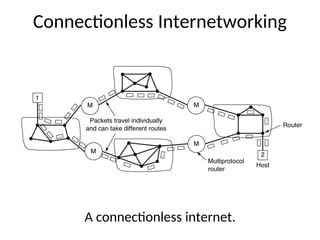
• Implementation of Connectionless Service
• Implementation of Connection-Oriented Service
• Comparison of Virtual-Circuit and Datagram Subnets
70. • Carrier equipment
• Store and forward packet switching
• The equipment is used as follows:
• A host with a packet to send transmits it to the nearest router,
either on its own LAN or over a point-to-point link to the carrier.
• The packet is stored there until it has fully arrived so the
checksum can be verified. Then it is forwarded to the next router
along the path until it reaches the destination host, where it is
delivered. This mechanism is called store-and-forward packet
switching.
71. Services Provided to the Transport Layer
The Network layer services are designed with the
following goals:
1. The services should be independent of the router
technology.
2. The transport layer should be shielded from the
number, type, and topology of the routers present.
3. The network addresses made available to the transport
layer should use a uniform numbering plan, even across
LANs and WANs.
Internet – Connection-less
ATM – Connection-oriented
72. Implementation of Connectionless
Service
.
1. If connection-less service is offered, packets are injected
into the subnet individually and routed independently of
each other.
2. No advance setup is needed.
3. In this context, the packets are called datagrams and the
subnet is called datagram subnet.
74. • Suppose that the process P1 has a long message for P2. It
hands the message to transport layer with instructions to
deliver it to process P2 on host H2.
• Let us assume that the message is four times longer than
the maximum packet size, so the network layer has to break
it into four packets, 1,2,3 and 4 and sends each of them in
turn to router A using point-to-point protocol, for example,
PPP. At this point the carrier takes over.
• Every router has an internal table telling it where to send
packets for each possible destination.
• Each table entry is a pair consisting of a destination and the
outgoing line to use for that destination. Only directly-
connected lines can be used.
75. • ‘A’ has only two out going lines- to B and C- so every incoming
packet must be sent to one of these routers, even if the ultimate
destination is some other router.
• A’s initial table is shown under the label “initially”.
• As they arrived at A, packets 1,2, and 3 were stored briefly( to verify
checksum). Then each was forwarded to C according to A’s table.
• Packet 1 was then forwarded to E and then to F. When it got to F, it
was encapsulated in a data link layer frame and sent to H2 over the
LAN. Packets 2 and 3 follow the same route.
• When packet 4 got to A it was sent to router B, even though it is also
destined for F.
• For some reason, A decided to send packet 4 via a different route.
Perhaps it learned of a traffic jam somewhere along ACE path and
updated its routing table as shown under the label “later”.
• The algorithm that manages the tables and makes the routing
decisions is called the Routing algorithm
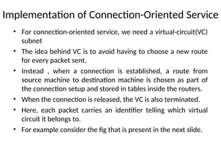
76. Implementation of Connection-Oriented Service
• For connection-oriented service, we need a virtual-circuit(VC)
subnet
• The idea behind VC is to avoid having to choose a new route
for every packet sent.
• Instead , when a connection is established, a route from
source machine to destination machine is chosen as part of
the connection setup and stored in tables inside the routers.
• When the connection is released, the VC is also terminated.
• Here, each packet carries an identifier telling which virtual
circuit it belongs to.
• For example consider the fig that is present in the next slide.
78. • Here, host H1 has established connection 1 with host H2.
• The first line of A’s table says that if a packet bearing
connection identifier 1 comes in from H1, it is to be sent to
router C and given connection identifier 1.
• Similarly, the first entry at C routes the packet to E, also with
connection identifier 1.
• Now let us consider what happens if H# also wants to establish
a connection to H2. It chooses connection identifier 1(because
it is initiating the connection and this is its only connection)
and tells subnet to establish the virtual circuit. This leads to
second row in the tables.
• We have a conflict here because although A can easily
distinguish connection 1 packets from H1 from connection 1
packets from H3, C cannot do this.
79. • For this reason, A assigns a different
connection identifier to the out going traffic
for the second connection.
• Avoiding conflicts of this kind is why routers
need the ability to replace connection
identifier in outgoing packets. This is called
Label switching.
80. Comparison of Virtual-Circuit and
Datagram Subnets
Inside the subnet, several trade-offs exist between virtual circuit
and data-grams.
• Router memory space and bandwidth
• Setup time versus address parsing time
• Amount of table space required in router memory
• Routing
• Quality of service
• Effect of router failure
• Congestion Control
84. • Correctness: The routing should be done properly and correctly so that the
packets may reach their proper destination.
• Simplicity: The routing should be done in a simple manner so that the
overhead is as low as possible. With increasing complexity of the routing
algorithms the overhead also increases.
• Robustness: Once a major network becomes operative, it may be expected
to run continuously for years without any failures. The algorithms designed
for routing should be robust enough to handle hardware and software
failures and should be able to cope with changes in the topology and traffic
without requiring all jobs in all hosts to be aborted and the network rebooted
every time some router goes down.
• Stability: The routing algorithms should be stable under all possible
circumstances.
• Fairness: Every node connected to the network should get a fair chance of
transmitting their packets. This is generally done on a first come first serve
basis.
• Optimality: The routing algorithms should be optimal in terms of throughput
and minimizing mean packet delays. Here there is a trade-off and one has to
choose depending on his suitability.
85. Routing Algorithms (2)
Conflict between fairness and optimality.
Minimizing the mean packet delay is an obvious candidate to
send traffic through the network effectively
A – A’, B – B’, C – C’, can fill the channel, then X-X’ doesn’t get a chance
86. Types of Routing Algorithms
• Routing Algorithms can be grouped into two major
classes:
1. Non-Adaptive(Static)
2. Adaptive(Dynamic)
• Non-Adaptive: They don’t base their routing decisions
on measurements or estimates of the current traffic and
topology. Instead the choice of the route is computed in
advance and downloaded to the routers when the
network is booted.
• Adaptive: They change their routing decisions to reflect
changes in the topology and usually traffic as well
87. Shortest Path Routing
• Here the idea is to build a graph of the subnet, with each node
of the graph representing a router and each arc of the graph
representing a communication line.
• In this algorithm, one way of measuring path length is no. of
hops, using this paths ABC & ABE are equally long.
• Another metric is geographic distance in kms. ABC is longer
than ABE.
• Other different metrics are also possible. For example, each
arc could be labeled with the mean queuing & transmission
delay for some standard test packets.
• Labels on arc can be computed as a function of distance,
Bandwidth, average traffic, communication cost, mean queue
length, measured delays and others.
88. Shortest Path Routing
• By Dijkstra, each node is labeled with its distance from source
node along the best known paths.
• Initially all nodes are labeled with infinity.
• A label may be either tentative or permanent.
• Initially all are tentative.
• When it is discovered that label represents a shortest possible
path from source to that node then it is made permanent &
never changed.
89. Shortest Path Routing
The first 5 steps used in computing the shortest path from A to D.
The arrows indicate the working node.
90. Dijkstra’s Algorithm to Compute The Shortest Path Through a
Graph
• Step 1: Plot the subnet, assign weights to each of the edges
between nodes.
• Step 2: Using the metrics as distance in km calculate
• the shortest path from the given source to destination.
• Step 3: Initially mark all the paths from source as infinity.
• Step4: Starting with the source node check the adjacent
nodes for shortest path, and mark them as tentative
nodes.
• Step 5: From this tentative nodes, select one which is having
short distance from source, and mark as permanent.
• Step 6: Distance from source to that tentative node should be
recorded.
• Step 7: Now this node is considered as source node and
• repeat the steps from 3 to 6.
• Step 8: Repeat the steps along the path with the distances
being added throughout the path to reach the
destination.
91. Flooding
Flooding is a static algorithm , in which every incoming packet is sent
out on every outgoing line except the one it arrived on.
It generates vast number of duplicate packets, an infinite number
unless some measures are taken.
• One such measure is to have a hop counter contained in the header of
each packet.
• Second is to keep track of which packets have been flooded, to avoid
sending them out a second time.
• Selective Flooding: Instead of sending every incoming packet on every
line, the packet is sent only on those lines that go in the right direction.
• Applications: In military application, Distributed database, in wireless
networks,
It can also be used as a metric against which other routing algorithms
can be compared.
92. Distance Vector Routing
• Modern computer networks use dynamic routing algorithms.
• DVR is a dynamic routing algorithm
• This algorithm operates by having each router maintain a
table(i.e, a vector) giving the best known distance to each
destination and which line to use to get there. These tables
are updated by exchanging information with the neighbors.
• This algorithm is some times called by other names, mostly
the distributed Bellman-Ford routing algorithm and Ford-
Fulkerson algorithms.
• In distance vector routing, each router maintains a routing
table indexed by, and containing one entry for, each router in
the subnet. This entry contains two parts: the preferred
outgoing line to use for that destination and an estimate of
the time or distance to that destination.
93. Distance Vector Routing
• The metrics can be number of hops, time delay in msecs,
total no.of packets queued along the path, or something
similar.
• If the metric is delay, the router can measure it directly with
special ECHO packets that the receiver just timestamps and
sends back as fast as it can.
• Assume that the metric is delay and that each router knows
the delay to each of its neighbors.
• Once every T msec each router sends to each neighbor a list
of its estimated delays to each destination. It also receives a
similar list from each neighbor.
• Imagine that one of these tables has just come in from
neighbor X, with Xi being X’s estimate of how long it takes to
get to router i.
94. Distance Vector Routing Algorithm :
Step 1: Plot the subnet showing the delay between the nodes.
Step 2: Construct the routing table for each node consisting of delay
to reach other nodes in the subnet and the line to be used.
Step 3: Each routers will calculate the delay to reach its adjacent
nodes. And this will be recorded in its routing table.
Step 4: Routing table will be exchanged among the routers for every T
seconds.
Step 5: Each router will wait until it receives an updated table from its
neighbors. For example, router A receives routing table from its
neighbor X, with Xi as the delay to reach I from X.
Step 6: With this information, A calculate the new routing table with a
delay of Xi+m to reach router I. Where m is a required time for A to
reach X.
Step 7: Router A will now can reach router I via X.
Step 8: This steps will be repeated for every source to every other
destination.
Step 9: Display routing table of each router.
96. Distance Vector Routing
• If the router knows that the delay to X is m msec, it also
knows that it can reach router i via X in Xi +m msec.
• By performing this calculation for each neighbor, a router
can find out which estimates seems the best and use that
estimate and corresponding line in its new routing table.
• Consider how J computes its new route to router G.
• JA= 8 msec, AG=18 msec, therefore J to G is 8+18=26 msec
via A.
• Similarly J to G via I, H and K as 41(31+10), 18(6+12), and
37(31+6) msec, respectively.
• The best of these values is 18, so it makes an entry in its
routing table that the delay to G is 18 msec and that the
route to use is via H.
• The same calculations are done for all other destinations
and a new routing table is constructed
97. Distance Vector Routing: The count-to-infinity problem
A is down
Then A comes up. The good news spreads quickly.
99. The count-to-infinity problem
• It should be clear why bad news travels slowly: no router ever
has a value more than one higher than the minimum of all its
neighbors
• Gradually, all the routers work their way up to infinity, but
the number of exchanges required depends on the numerical
value used for infinity.
• For this reason, it is wise to set infinity to the longest path
plus 1 (if using hop count as metric).
• If the metric is time delay, there is no well-defined upper
bound, so a high value is needed to prevent a path with a long
delay from being treated as down
100. • Partial Solutions:
• Make infinity small
• -use for example16 to represent infinity
• Split Horizon
• -Don’t send routes learnt from a neighbor back to it.
• Split Horizon with poison reverse
• -Send routes learnt from a neighbor back to it but with
infinite cost
101. Link State Routing
1. Distance vector routing was used in the ARPANET until 1979,
then it was replaced by link state routing.
2. Two primary reasons caused its demise
3. First, since the delay metric was queue length, it did not take
line bandwidth into account when choosing routes
4. Second, the algorithm often took too long to converge(the
count-to-infinity problem).
5. For these reasons, it was replaced by an entirely new
algorithm now called link state routing.
6. It is also available in two variants
1.IS-IS(Intermediate System-Intermediate System)
2.OSPF(Open Shortest Path First)
102. Link State Routing
Each router must do the following:
1. Discover its neighbors, learn their network address.
2. Measure the delay or cost to each of its neighbors.
3. Construct a packet telling all it has just learned.
4. Send this packet to all other routers.
5. Compute the shortest path to every other router.
103. Link State Routing
• Distance vector routing differs significantly from
the link state routing.
• With link state algorithms, routers share only the
identity of their neighbors, but they flood this
information through the entire network. Distance
vector algorithms adopt an opposite approach.
Routers periodically share knowledge of the entire
network, but only with their neighbors
• Link state routing requires more memory and
computation
104. Link State Routing
Learning about the Neighbors
• When a router is booted, its first task is to learn who
its neighbor are. It accomplishes this goal be sending
a special HELLO packet on each point-to-point line.
The router on the other end is expected to send back
a reply telling who it is
• When two or more routers are connected by a LAN,
the situation is slighted more complicated. One way
to model the LAN is to consider it as a node itself
105. Learning about the Neighbors
…………….By sending HELLO packets
(a) Nine routers and a LAN. (b) A graph model of (a).
106. Link State Routing
Measuring Line Cost
• The link state routing algorithm requires each router
to know, or at least have a reasonable estimate, of
the delay to each of its neighbors.
• The most direct way to determine this delay is to
send a special ECHO packet over the line that the
other side is required to send back immediately.
• By measuring the round-trip time and dividing it by
two, the sending router can get a reasonable
estimate of the delay
107. Link State Routing
Measuring Line Cost
• An interesting issue is whether or not to take the load into
account when measuring the delay.
• To factor the load in, the round-trip timer must be started
when the ECHO packet is queued.
• To ignore the load, the timer should be started when the ECHO
packet reaches the front of the queue.
108. Measuring Line Cost
A subnet in which the East and West parts are connected by two lines.
109. • ECHO packet
• RTT/2
• An important issue is whether to take load into account when measuring
the delay.
• To factor in ,RTT must be started when ECHO packet is queued.
• To ignore the load, the timer should be started when the ECHO packet
reaches the front of queue.
• Two arguments:
• Including traffic-induced delays in the measurement.
• Including load in delay calculation.
• The best solution is to distribute the load over multiple lines, with some
known fraction going over each line.
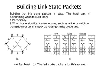
110. Building Link State Packets
(a) A subnet. (b) The link state packets for this subnet.
Building the link state packets is easy. The hard part is
determining when to build them.
1.Periodically
2.When some significant event occurs, such as a line or neighbor
going down or coming back up ,changes in its properties.
111. Link State Routing
•Distributing the Link State Packets
•The trickiest part of the algorithm is distributing the
link state packets reliably. As the packets are
distributed and installed, the routers getting the first
ones will change their routes.
•Consequently, the different routers may be using
different versions of the topology, which can lead to
inconsistencies, loops, unreachable machines, and
other problems.
•The fundamental idea is to use flooding to distribute
the link state packets
112. Link State Routing
Distributing the Link State Packets
• To keep the flood in check, each packet contains a sequence
number that is incremented for each new packet sent. Routers
keep track of all the (source router, sequence) pairs they see.
• When a new link state packet comes in, it is checked against the
list of packets already seen.
• 1. If new: forward on all lines except the one it arrived
on
• 2. If duplicate or old packet: discard
113. Link State Routing
Distributing the Link State Packets & its problems
• If the sequence numbers wrap around, confusion will reign.
The solution here is to use a 32-bit sequence number. With
one link state packet per second, it would take 137 years to
wrap around.
• If a router ever crashes, it will lose track of its sequence
number. If it starts again at 0, the next packet will be rejected
as a duplicate.
• If a sequence number is ever corrupted and 65540 is received
instead of 4 (a 1-bit error), packets 5 through 65540 will be
rejected as obsolete, since the current sequence number is
thought to be 65,540.
114. Link State Routing
Distributing the Link State Packets
• The solution to all these problems is to include the age of each
packet after the sequence number and decrement it once per
second. When the age hits zero, the information from that router
is discarded.
• The age field is also decremented by each router during the initial
flooding process, to make sure no packet can get lost and live for
an indefinite period of time.
Refinement:
• When a link State packet comes in to a router for flooding, it is not
queued for transmission immediately. Instead it is first put in
holding area. If another packet from same source comes in before
the first packet is transmitted, their sequence numbers are
compared.
115. Distributing the Link State Packets
To guard against errors on the router-router lines, all
link state packets are acknowledged.
Packet buffer for router B
Link State Routing
116. Link State Routing
Computing the New Routes
• Once a router has accumulated a full set of link state packets, it
can construct the entire subnet graph because every link is
represented. Now Dijkstra’s algorithm can be run locally to
construct the shortest path to all possible destinations.
• The OSPF (Open Shortest Path First) protocol uses link state
routing algorithm
• Another link state is IS-IS, was used in connectionless network
layer protocol
118. Hierarchical Routing
• Unfortunately, the gain in routing table space are not free.
There is a penalty to be paid, and this penalty is in the form of
increased path length.
For example, the best route from 1A to 5C is via region 2,
but with hierarchical routing all traffic to region 5 goes via
region 3, because that is better for most destinations in
region.
• Consider a subnet with 720 routers. If there is no hierarchy,
each router needs 720 routing table entries.
119. Hierarchical Routing
• If the subnet is partitioned into 24 regions of 30 routers each,
each router needs 30 local entries plus 23 remote entries for a
total of 53 entries.
• If a three level hierarchy is chosen, with eight clusters, each
containing 9 regions of 10 routers, each router needs 10 entries
for local routers, 8 entries for routing to other regions within its
own cluster, and 7 entries for distant clusters, for a total of 25
entries.
• Kamoun and kleinrock discovered that the optimal number of
levels for an N router subnet is ln N, requiring a total of e ln N
entries per router.
120. Broadcast Routing
• One broadcasting method that requires no special features from the
subnet is for the source to simply send a distinct packet to each
destination.
• Waste bandwidth and require the source to have a complete list of
all destinations.
• Flooding is another obvious candidate. But it generates too many
packets and consumes too much bandwidth
121. Broadcast Routing: Multi destination routing
• Each packet contains either a list of destinations or a bit map
indicating the desired destinations. When a packet arrives at a
router, the router checks all the destinations to determine the set
of output lines that will be needed.
• The router generates a new copy of the packet for each output line
to be used and includes in each packet only those destinations that
are to use the line. In effect, the destination set is partitioned
among the output lines
122. Broadcast Routing
• A fourth broadcast algorithm makes explicit use of the
sink tree for the router initiating the broadcast, or any
other convenient spanning tree for that matter
• This method makes excellent use of bandwidth,
generating the absolute minimum number of packets
necessary to do the job. The only problem is that each
router must have knowledge of some spanning tree for
it to be applicable
123. Broadcast Routing: Reverse Path Forwarding
• When a broadcast packet arrives at a router, the router
checks to see if the packet arrived on the line that is
normally used for sending packets to the source of the
broadcast. If so, forward it.
Reverse path forwarding. (a) A subnet. (b) a Sink tree. (c) The tree built by
reverse path forwarding.
124. Multicast Routing
• To do multicasting, group management is required. Some way
is needed to create and destroy groups, and for processes to
join and leaves groups. It is important that routers know
which of their hosts belong to which groups.
• Either hosts must inform their routers about changes in group
membership, or routers must query their hosts periodically.
Either way, routers learn about which of their hosts are in
which groups. Routers tell their neighbors, so the
information propagates through the subnet
125. Multicast Routing
• To do multicast routing, each router computes a spanning
tree covering all other routers in the subnet
A multicast tree for group 1
126. Multicast Routing
(a) A network. (b) A spanning tree for the leftmost router.
(c) A multicast tree for group 1. (d) A multicast tree for group 2.
127. Multicast Routing
• Various ways of pruning the spanning tree are possible. The
simplest one can be used if link state routing is used, and
each router is aware of the complete subnet topology,
including which hosts belong to which groups.
• Then the spanning tree can be pruned by starting at the end
of each path and working toward the root, removing all
routers that do not belong to the group in question.
128. Multicast Routing
• With distance vector routing, a different strategy is used. The basic
algorithm is Distance vector algorithm whenever a router with no
hosts interested in a particular group and no connections to other
routers receives a multicast message for that group, it responses
with a PRUNE message, telling the sender not to send it any more
multicasts for that group
• source-specific multicast trees: scales poorly to large networks n
groups, m members: a total of nm trees
• core-based tree approach: each group has only one multicast tree
n groups: n trees
129. Internetworking
• How Networks Differ
• How Networks Can Be Connected
• Concatenated Virtual Circuits
• Connectionless Internetworking
• Tunneling
• Internetwork Routing
• Fragmentation
132. How Networks Can Be Connected
• Networks can be interconnected by different devices.
• In PL, Repeaters or hubs can be used
• In DLL, Bridges and Switches can be used.(examines MAC address,
do minor translations).
• In NL, Routers can be used( if differ they are able to translate
between packet formats, which is rare). A router that can handle
multiple protocols is called a multiprotocol router.
• In TL & AL gateways do translation.
133. How Networks Can Be Connected
(a) Two Ethernets connected by a switch.
(b) Two Ethernets connected by routers.
138. The Network Layer in the Internet
1. Make sure it works: Do not finalize the design or standard
until multiple prototypes have successfully communicated
with each other.
2. Keep it simple: When in doubt, use the simplest solution. If
a feature is not absolutely essential, leave it out, especially if
the same effect can be achieved by combining other features.
139. 3. Make clear choices: If there are several ways of doing the
same thing, choose one.
4 . Exploit modularity: This principle leads directly to the idea
of having protocol stacks, each of whose layers is
independent of all the other ones. In this way, if
circumstances that require one module or layer to be changed,
the other ones will not be affected.
5. Expect heterogeneity: Different types of hardware,
transmission facilities, and applications will occur on any
large network. To handle them, the network design must be
simple, general, and flexible.
140. 6. Avoid static options and parameters: If parameters are
unavoidable (e.g., maximum packet size), it is best to have the
sender and receiver negotiate a value than defining fixed
choices.
7. Look for a good design; it need not be perfect: Often the
designers have a good design but it cannot handle some weird
special case. Rather than messing up the design, the designers
should go with the good design and put the burden of working
around it on the people with the strange requirements.
8. Be strict when sending and tolerant when receiving: In other
words, only send packets that rigorously comply with the
standards, but expect incoming packets that may not be fully
conformant and try to deal with them.
141. 9. Think about scalability: If the system is to handle millions of
hosts and billions of users effectively, no centralized databases
of any kind are tolerable and load must be spread as evenly as
possible over the available resources.
10.Consider performance and cost: If a network has poor
performance or outrageous costs, nobody will use it.
• Let us now leave the general principles and start looking at the
details of the Internet's network layer. At the network layer,
the Internet can be viewed as a collection of sub networks or
Autonomous Systems (ASes) that are interconnected.
• There is no real structure, but several major backbones exist.
These are constructed from high-bandwidth lines and fast
routers. Attached to the backbones are regional (midlevel)
networks, and attached to these regional networks are the
LANs at many universities, companies, and Internet service
providers.
142. The Network Layer in the Internet (2)
The Internet is an interconnected collection of many networks.
143. What is an IP Address?
• An IP address is a unique global address for a
network interface
• It is a 32 bit long identifier
• An IP address contains two parts:
- network number (network prefix)
- host number
144. Dotted Decimal Notation
• IP addresses are written in a so-called dotted
decimal notation
• Each byte is identified by a decimal number in
the range [0..255]:
• Example:
10001111
10000000 10001001 10010000
1st
Byte
= 128
2nd
Byte
= 143
3rd
Byte
= 137
4th
Byte
= 144
128.143.137.144
145. • Example:
• Network id is: 128.143
• Host number is: 137.144
• Prefix notation: 128.143.137.144
» Network prefix is 16 bits long
Example
128.143 137.144
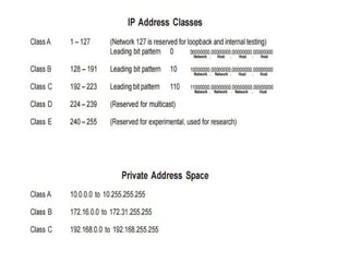
146. Class full IP Addresses
• The Internet address space was divided up into classes:
• Class A addressing – Allow 128 networks and 16 millions
hosts .
• Class B addressing – Allows 16,384 networks with 65,534
hosts.
• Class C addressing – 2 million networks with 254 hosts.
• Class D addressing- number of groups are 2^28 million
groups
• Class E addressing: Future purpose
149. IPv4 Addresses
• An IP address is a 32-bits long
• The IP addresses are unique and universal
• The address space of IPv4 is 232
or 4,294,967,296
• Binary notation: 01110101 10010101 00011101 00000010
• Dotted-decimal notation: 117.149.29.2
150. Example
• Change the following IP addresses from binary notation to dotted-decimal
notation.
a. 10000001 00001011 00001011 11101111
b. 11111001 10011011 11111011 00001111
We replace each group of 8 bits with its equivalent decimal number and add
dots for separation:
a. 129.11.11.239
b. 249.155.251.15
151. Classful addressing
• In classful addressing, the address space is divided into five classes: A, B, C, D, E
• A new architecture, called classless addressing was introduced in the mid-1990s
152. Classful Addressing: Example
• Find the class of each address.
a. 00000001 00001011 00001011 11101111
b. 11000001 10000011 00011011 11111111
c. 14.23.120.8
d. 252.5.15.111
• Solution
a. The first bit is 0. This is a class A address.
b. The first 2 bits are 1; the third bit is 0. This is a class C address.
c. The first byte is 14; the class is A.
d. The first byte is 252; the class is E.
154. Classes and Blocks
• In classful addressing, a large part of the available addresses were wasted
155. Netid and Hostid
• IP address in classes A, B, and C is divided into netid and hostid
156. Mask: Default Mask
• The length of the netid and hostid is predetermined in classful addressing
• Default masking
• CIDR (Classless Interdomain Routing) notation
157. Computer Networks 19-157
Subnetting
• Combine several class C blocks to create a larger range of addresses
• Decrease the number of 1s in the mask (/24 /22 for C addresses)
Supernetting
• Divide a large block of addresses into several contiguous groups and assign each
group to smaller networks called subnets
• Increase the number of 1s in the mask
161. Computer Networks 19-161
Classless addressing: CIDR
• Classful addressing has created many problems
• Many ISPs and service users need more addresses
• Idea is to have variable-length blocks that belong to no class
• Three restrictions on classless address blocks;
– The addresses in a block must be contiguous, one after another
– The number of addresses in a block must be a power of 2
– The first address must be evenly divisible by the number of addresses
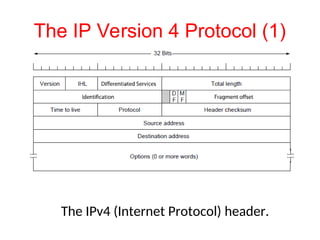
165. The IP Version 4 Protocol (1)
The IPv4 (Internet Protocol) header.
166. • Version:(4 bits): The Version field keeps track of which
version of the protocol the datagram belongs to.
• Internet Header Length(IHL 4 bits): IHL, is provided to tell
how long the header is, in 32-bit words. The minimum value is
5, which applies when no options are present. The maximum
value of this 4-bit field is 15, which limits the header to 60
bytes, and thus the Options field to 40 bytes.
• Type-of-Service (8 bits): The Type of service field is one of
the few fields that has changed its meaning (slightly) over the
years. It was and is still intended to distinguish between
different classes of service. Various combinations of reliability
and speed are possible. For digitized voice, fast delivery beats
accurate delivery. For file transfer, error-free transmission is
more important than fast transmission.
167. • Originally, the 6-bit field contained (from left to right), a
three-bit Precedence field and three flags, D, T, and R. The
Precedence field was a priority, from 0 (normal) to 7 (network
control packet). The three flag bits allowed the host to specify
what it cared most about from the set {Delay, Throughput,
Reliability}.
• Total length(16 bits): The Total length includes everything in
the datagram—both header and data. The maximum length is
65,535 bytes. At present, this upper limit is tolerable, but with
future gigabit networks, larger data grams may be needed.
169. • Identifier (16 bits): To have a proper reassembling of
fragments , The Identification field is needed to allow the
destination host to determine which datagram a newly arrived
fragment belongs to. All the fragments of a datagram contain
the same Identification value.
• Flags(3 bits): First one an unused bit Only two of the bits are
currently defined: MF(More Fragments) ,DF(Don't Fragment)
MF(More Fragments) :When a receiving host sees a packet
arrive with the MF = 1, it examines the Fragment Offset to see
where this fragment is to be placed in the reconstructed
packet.
Don't Fragment flag (DF):The Don't Fragment (DF) flag is a
single bit in the Flag field that indicates that fragmentation of
the packet is not allowed.
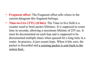
170. • Fragment offset: The Fragment offset tells where in the
current datagram this fragment belongs.
• Time-to-Live (TTL) (8 bits): The Time to live field is a
counter used to limit packet lifetimes. It is supposed to count
time in seconds, allowing a maximum lifetime of 255 sec. It
must be decremented on each hop and is supposed to be
decremented multiple times when queued for a long time in a
router. In practice, it just counts hops. When it hits zero, the
packet is discarded and a warning packet is sent back to the
source host..
171. • Protocol (8 bits): The Protocol field tells it which transport
process to give it to. TCP is one possibility, but so are UDP
and some others.
• Header checksum (16 bits): The Header checksum verifies
the header only. Such a checksum is useful for detecting errors
generated by bad memory words inside a router.
173. • IP Destination Address (32 bits): The IP Destination
Address field contains a 32-bit binary value that represents the
packet destination Network layer host address.
• IP Source Address (32 bits): The IP Source Address field
contains a 32-bit binary value that represents the packet source
Network layer host address.
• Options (variable): The Options field is padded out to a
multiple of four bytes. Originally, five options were defined
The current complete list is now maintained on-line at
www.iana.org/assignments/ip-parameters.
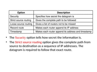
174. • The Security option tells how secret the information is.
• The Strict source routing option gives the complete path from
source to destination as a sequence of IP addresses. The
datagram is required to follow that exact route.
175. • The Loose source routing option requires the packet to
traverse the list of routers specified, and in the order specified,
but it is allowed to pass through other routers on the way.
• The Record route option tells the routers along the path to
append their IP address to the option field. This allows system
managers to track down bugs in the routing algorithms.
• Finally, the Timestamp option is like the Record route option,
except that in addition to recording its 32-bit IP address, each
router also records a 32-bit timestamp. This option, too, is
mostly for debugging routing algorithms.
177. The Main IPv6 Header
The IPv6 fixed header (required).
178. Computer Networks 20-178
IPv6 address
• The use of address space is inefficient
• Minimum delay strategies and reservation of resources are required to
accommodate real-time audio and video transmission
• No security mechanism (encryption and authentication) is provided
• IPv6 (IPng: Internetworking Protocol, next generation)
– Larger address space (128 bits)
– Better header format
– New options
– Allowance for extention
– Support for resource allocation: flow label to enable the source to request
special handling of the packet
– Support for more security
179. Computer Networks 20-179
IPv6 Datagram
• IPv6 defines three types of addresses: unicast, anycast (a group of computers with
the same prefix address), and multicast
• IPv6 datagram header and payload
181. Computer Networks 20-181
IPv6 Header
• Version: IPv6
• Priority (4 bits): the priority of the packet with respect to traffic congestion
• Flow label (3 bytes): to provide special handling for a particular flow of data
• Payload length
• Next header (8 bits): to define the header that follows the base header in the
datagram
• Hop limit: TTL in IPv4
• Source address (16 bytes) and destination address (16 bytes): if source routing is
used, the destination address field contains the address of the next router
182. Computer Networks 20-182
Priority
• IPv6 divides traffic into two broad categories: congestion-controlled and
noncongestion-controlled
• Congestion-controlled traffic
• Noncongestion-controlled traffic
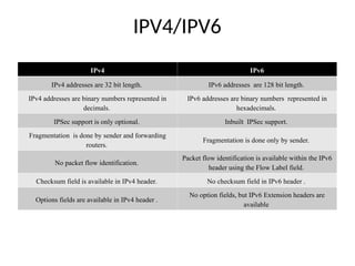
186. IPV4/IPV6
IPv4 IPv6
IPv4 addresses are 32 bit length. IPv6 addresses are 128 bit length.
IPv4 addresses are binary numbers represented in
decimals.
IPv6 addresses are binary numbers represented in
hexadecimals.
IPSec support is only optional. Inbuilt IPSec support.
Fragmentation is done by sender and forwarding
routers.
Fragmentation is done only by sender.
No packet flow identification.
Packet flow identification is available within the IPv6
header using the Flow Label field.
Checksum field is available in IPv4 header. No checksum field in IPv6 header .
Options fields are available in IPv4 header .
No option fields, but IPv6 Extension headers are
available
188. Internet Control Message Protocol
• The operation of the internet is monitored by
the routers.
• When something unexpected occurs, the event
is reported by ICMP, which is also used to test
the internet.
190. ARP– The Address Resolution
Protocol
• Although every machine on the Internet has IP address,This cannot actually be used
for sending packets because DL layer hardware does not understand Internet address.
• How do IP address get mapped onto data-link layer address, such as Ethernet?
• A host 1 sends a packet to a user on host 2.
• Let us assume sender knows name of the receiver.
• The first step is to find out IP address of H2, which is done by DNS.
• Now H1 builts a packet with destination address H2 IP address.
• But now it need a technique to find out Destination’s Ethernet address.
• One solution is to have a configuration file that could do the mapping, but it is error-
prone & time-consuming job.
• The better solution is to use a protocol called ARP(Address Resolution Protocol), which
finds out Ethernet address corresponding to a given IP address.
191. ARP– The Address Resolution
Protocol
Three interconnected /24 networks: two Ethernets and an FDDI ring.
192. ARP contd..
• The advantage is its simplicity.
• Optimization made to ARP:
• once a machine runs ARP, it caches the results in case it needs to contact the same
machine shortly.
• Next time it will find mapping in its own cache, thus eliminates second broadcast
• Another is to have every machine broadcast its mapping when it boots
• In the above, Suppose H1 wants to send packet to H4.
• Using ARP will fail, bcoz H4 will not see this broadcast msg.
• There are two solutions..
• 1. CS router could be configured to respond to ARP request for the network
192.31.63.0.
• H1 will make an ARP cache entry of (192.31.63.8, E3) and sends all traffic for
H4 to local router. This solution is called proxy ARP.
• 2. H1 immediately see that the destination is on a remote network and just send all
such traffic to a default Ethernet address that handles all remote traffic, in this case
E3
193. RARP and BOOTP
• Reverse Address Resolution protocol(RARP) allows a newly-booted workstation
to broadcast its Ethernet address, and RARP server sees this request, looks up the
Ethernet address in its configuration files, and sends back the corresponding IP
address.
• A disadvantage of this is it uses a destination address of all 1’s to reach the RARP
server. However such broadcast are not done forwarded by routers, so RARP
server is needed on each network.
• An alternative bootstrap protocol called BOOTP was used
• BOOTP uses UDP messages, which are forwarded over routers.
• It also provides a diskless workstation, including IP address of the file server
holding memory image, IP address of the default router, and the subnet mask to
use
• BOOTP requires manual configuration of tables mapping IP address to Ethernet
address
194. Dynamic Host Configuration
Protocol
• DHCP allows both manual IP address assignment and automatic assignment.
• Uses special server that assign IP address, it is need not be on same LAN as the
requesting host.
• DHCP server cannot be reachable by broadcasting, a DHCP relay agent is needed on
each LAN.
• To find IP address, a new machine broadcasts a DHCP DISCOVER packet.
• The relay agent intercepts the broadcast messages. When it finds DHCP DISCOVER
packet, it sends the packet as a uni-cast packet to DHCP server(Relay agent needs to
know IP address of DHCP server).
• An issue is how long an IP address should be allocated.
• Uses a technique called Leasing.
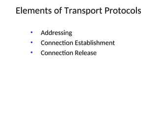
201. Transport Service Primitives (3)
A state diagram for a simple connection management scheme.
Transitions labeled in italics are caused by packet arrivals. The
solid lines show the client's state sequence. The dashed lines show
the server's state sequence.
207. Connection Establishment (3)
Three protocol scenarios for establishing a connection using a
three-way handshake. CR denotes CONNECTION REQUEST.
(a) Normal operation,
(b) Old CONNECTION REQUEST appearing out of nowhere.
(c) Duplicate CONNECTION REQUEST and duplicate ACK.
210. Connection Release (3)
Four protocol scenarios for releasing a connection. (a) Normal case of a
three-way handshake. (b) final ACK lost.
6-14, a, b
214. The Internet Transport Protocols: TCP
• Introduction to TCP
• The TCP Service Model
• The TCP Protocol
• The TCP Segment Header
• TCP Connection Establishment
• TCP Connection Release
215. The TCP Service Model
Some assigned ports.
Port Protocol Use
21 FTP File transfer
23 Telnet Remote login
25 SMTP E-mail
69 TFTP Trivial File Transfer Protocol
79 Finger Lookup info about a user
80 HTTP World Wide Web
110 POP-3 Remote e-mail access
119 NNTP USENET news
216. The TCP Service Model (2)
(a) Four 512-byte segments sent as separate IP datagrams.
(b) The 2048 bytes of data delivered to the application in a single
READ CALL.
221. DNS – The Domain Name System
• The DNS Name Space
• Resource Records
• Name Servers
222. DNS
• DNS is the invention of a hierarchical, domain-
based naming scheme and a distributed
database system for implementing the naming
scheme.
• DNS is used to map a name onto an IP address,
an application program calls a library procedure
called the Resolver, passing it the name as a
parameter.
223. The DNS Name Space
A portion of the Internet domain name space.
224. DNS Name Space
• Internet is divided into 200 top-level domains, where each
domain covers many hosts.
• Each domain is partitioned into subdomains, and these are
further partitioned, and so on.
• Top-level domains : Generic
• Countries.
• Generic Domains were com(commercial), edu(educational
institutions), gov, int(international organizations), mil,
net(network providers), and org(non profit organization).
• The Country domains include one entry for every country.
• Each domain is named by the path upward from it to the
(unnamed) root.
225. DNS(contd..)
• Domain names can be either absolute or relative.
• An absolute domain name always ends with a period
(e.g.,eng.sun.com)
• Relative does not.
• Domain names are case insensitive.
• Domains can be inserted into the tree in two different ways.
• Each domain controls how it allocates the domains under it.
• To create a new domain, permission is required of the domain
in which it will be included. So that name conflicts are avoided.
• Once domain has been created & registered, it can create
subdomains, without getting permission from anybody higher
up the tree.
226. Resource Records
• Every Domain, whether it is a single host or a top-level domain, can
have a set of resource records associated with it.
• For single host, the most common resource record is just its IP
address, but many other kinds of resource records also exist.
• When a resolver gives a domain name to DNS, it gets back resource
records associated with that name. Thus, the primary function of
DNS is to map domain names onto resource records.
• A resource record is a five-tuple. The format is as follows:
• Domain_name Time_to_live Class Type Value
• Domain_name :tells the domain to which this record applies
• Time_to_live field gives an indication of how stable the record is.
• Class: For Internet information, it is always IN
• For non-Internet information, other codes can be used.
227. Resource Records
Type: This field tells what kind of record this is. The important types are
listed below
The principal DNS resource records types.
Value: This can be a number, a domain name, or an
ASCII string.
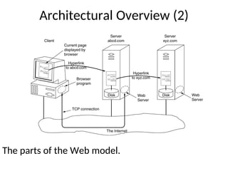
231. The World Wide Web
• Architectural Overview
• Static Web Documents
• Dynamic Web Documents
• HTTP – The HyperText Transfer Protocol
• Performance Ehnancements
• The Wireless Web
234. Computer Networks 27-234
Architecture of WWW
•The WWW today is a distributed client/server service, in which a client using a browser
can access a service using a server. However, the service provided is distributed over
many locations called sites.


![Dotted Decimal Notation
• IP addresses are written in a so-called dotted
decimal notation
• Each byte is identified by a decimal number in
the range [0..255]:
• Example:
10001111
10000000 10001001 10010000
1st
Byte
= 128
2nd
Byte
= 143
3rd
Byte
= 137
4th
Byte
= 144
128.143.137.144](https://image.slidesharecdn.com/jntuhs-18-12-2024-copy-250627021544-16b9b44e/85/JNTUHS-18-12-2024-Copy-ppt-computer-networks-notes-144-320.jpg)