L21_L27_Unit_5_Dynamic_Programming Computer Science

• Useful for solving multistage optimization problems.
• An optimization problem deals with the maximization or minimization
of the objective function as per problem requirements.
• In multistage optimization problems, decisions are made at successive
stages to obtain a global solution for the given problem.
• Dynamic programming divides a problem into subproblems and
establishes a recursive relationship between the original problem and
its subproblems.
BASICS OF DYNAMIC PROGRAMMING
2

BASICS OF DYNAMIC PROGRAMMING-cont’d
• A subproblem representing a small part of the original problem is
solved to obtain the optimal solution.
• Then the scope of this subproblem is enlarged to find the optimal
solution for a new subproblem.
• This enlargement process is repeated until the subproblem’s scope
encompasses the original problem.
• After that, a solution for the whole problem is obtained by combining
the optimal solutions of its subproblems.
3

• The difference between dynamic programming and the top-down or divide-and-conquer approach is that the
subproblems overlap in the dynamic programming approach. In contrast, in the divide-and-conquer
approach, the subproblems are independent. The differences between the dynamic programming and
divide-and-conquer approaches.
Dynamic programming vs divide-and-conquer
approaches
4

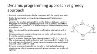
Dynamic programming approach vs greedy
approach
• Dynamic programming can also be compared with the greedy approach.
• Unlike dynamic programming, the greedy approach fails in many
problems.
• consider the shortest-path problem for the distance between s and t in
the graph shown in Fig. A greedy algorithm such as Dijkstra would take
the route from s to vertex 2, as its path length is shorter than that of the
route from s to ‘1’.
• After that, the path length increases, resulting in a total path length of
1002.
• However, dynamic programming would not make such a mistake, as it
treats the problem in stages.
• For this problem, there are three stages with vertices {s}, {1, 2}, and {t}.
The problem would find the shortest path from stage 2, {1, 2}, to {t} first,
then calculate the final path. Hence, dynamic programming would result
in a path s to 1 and from 1 to t.
• Dynamic programming problems, therefore, yield a globally optimal
result compared to the greedy approach, whose solutions are just locally
optimal.
5

Dynamic programming approach vs greedy approach
Advantages and Disadvantages of dynamic programming
6

Components of Dynamic Programming
• The guiding principle of dynamic programming is the ‘principle of optimality’. In
simple words, a given problem is split into subproblems.
• Then, this principle helps us solve each subproblem optimally, ultimately leading
to the optimal solution of the given problem. It states that an optimal sequence
of decisions in a multistage decision problem is feasible if its sub-sequences are
optimal.
• In other words, the Bellman principle of optimality states that “an optimal policy
(a sequence of decisions) has the property that whatever the initial state and
decision are, the remaining decisions must constitute an optimal policy
concerning the state resulting from the first decision”.
• The solution to a problem can be achieved by breaking the problem into
subproblems. The subproblems can then be solved optimally. If so, the original
problem can be solved optimally by combining the optimal solutions of its
subproblems.
7

Components of Dynamic Programming
8

overlapping subproblems
• Dynamic programs possess two essential properties—
• overlapping subproblems
• optimal substructures.
• Overlapping subproblems One of the main characteristics of dynamic
programming is to split the problem into subproblems, similar to the
divide-and-conquer approach. The sub-problems are further divided into
smaller problems. However, unlike divide and conquer, here, many
subproblems overlap and cannot be treated distinctly.
• This feature is the primary characteristic of dynamic programming. There
are two ways of handling this overlapping problem:
• The memoization technique
• The tabulation method.
9

overlapping subproblems
• The Fibonacci sequence is given as (0, 1, 1, 2, 3, 5, 8, 13, …). The
following recurrence equations can generate this sequence:
𝐹0 = 0
𝐹1 = 1
𝐹𝑛 = 𝐹𝑛−1 + 𝐹𝑛−2 𝑓𝑜𝑟 𝑛 ≥ 2
• A straightforward pseudo-code for implementing this recursive
equation is as follows:
• Consider a Fibonacci recurrence tree for n = 5, as shown in Fig. 13.2.
• It can be observed from Fig. 13.3 that there are multiple overlapping
subproblems.
• As n becomes large, subproblems increase exponentially, and
repeated calculation makes the algorithm ineffective. In general, to
compute Fibonacci(n), one requires two terms:
• Fibonacci (n-1) and Fibonacci (n-2)
• Even for computing Fibonacci(50), one must have all the previous 49
terms, which is tedious.
• This exponential complexity of Fibonacci computation is because many
of the subproblems are repetitive, and hence there are chances of
multiple recomputations.
• The complexity analysis of this algorithm yields 𝑇 𝑛 = Ω 𝜙𝑛 . Here f
is called the golden ratio, whose value is approximately 1.62. 10

Optimal substructure
• The optimal solution of a problem can be expressed in terms of optimal
solutions to its subproblems.
• In dynamic programming, a problem can be divided into subproblems.
Then, the subproblem can be solved suboptimally. If so, the optimal
solutions of the subproblems can lead to the optimal solution of the
original problem.
• If the solution to the original problem has stages, then the decision taken
at the current stage depends on the decision taken in the previous stages.
• Therefore, there is no need to consider all possible decisions and their
consequences as the optimal solution of the given problem is built on the
optimal solution of its subproblems
11

• Consider the graph shown in Fig. 13.3. Consider the best route to visit the
city v from city u.
• This problem can be broken into a problem of finding a route from u to x
and from x to v. If <u, x> is the optimal route from u to x, and the best
route from x to v is <x, v>, then the best route from u to v can be built on
the optimal solutions of its two subproblems. In other words, the route
constructed on the suboptimal optimal routes must also be optimal.
• The general template for solving dynamic programming looks like this:
• Step 1: The given problem is divided into many subproblems, as in the case
of the divide-and-conquer strategy. In divide and conquer, the subproblems
are independent of each other; however, in the dynamic programming
case, the subproblems are not independent of each other, but they are
interrelated and hence are overlapping subproblems.
12

• Step 2: A table is created to avoid the recomputation of multiple
overlapping subproblems repeatedly; a table is created. Whenever a
subproblem is solved, its solution is stored in the table, so that its solutions
can be reused.
• Step 3.The solutions of the subproblems are combined in a bottom-up
manner to obtain the final solution of the given problem
• The essential steps are thus:
1. It is breaking the problems into its subproblems.
2. Creating a lookup table that contains the solutions of the subproblems.
3. Reuse the solutions of the subproblems stored in the table to construct
solutions to the given problem.
13

Dynamic programming uses the lookup table in both a top-down manner
and a bottom-up manner. The top-down approach is called the
memorization technique, and the bottom-up manner is called the tabulation
method.
1. Memoization technique: This method looks into a table to check whether
the table has any entries. The lookup table Contains entries such as ‘NIL’ or
‘undefined’. If no value is present, then it is computed. Otherwise, the pre-
computed value is reused. In other words, computation follows a top-down
method similar to the recursion approach.
2. Tabulation method: Here, the problem is solved from scratch. The
smallest subproblem is solved, and its value is stored in the table. Its value is
used later for solving larger problems. In other words, computation follows a
bottom-up method.
14

FIBONACCI PROBLEM
• The Fibonacci sequence is given as (0, 1, 1, 2, 3, 5, 8, 13, …). The following
recurrence equations can generate this sequence:
𝐹0 = 0
𝐹1 = 1
𝐹𝑛 = 𝐹𝑛−1 + 𝐹𝑛−2 𝑓𝑜𝑟 𝑛 ≥ 2
• The best way to solve this problem is to use the dynamic programming
approach, in which the results of the intermediate problems are stored.
Consequently, results of the previously computed subproblems can be used
instead of recomputing the subproblems repeatedly. Thus, a subproblem is
computed only once, and the exponential algorithm is reduced to a
polynomial algorithm.
• A table is created to store the intermediate results, a table is created, and
its values are reused.
15

Bottom-up approach
• An iterative loop can be used to modify this Fibonacci number computation
effectively, and the resulting dynamic programming algorithm can be used to
compute the nth Fibonacci number.
• Step 1: Read a positive integer n.
• Step 2: Initialize first to 0.
• Step 3: Initialize second to 1.
• Step 4: Repeat n − 1 times.
• 4a: Compute current as first + second.
• 4b: Update first = second.
• 4c: Update second = current.
• Step 5: Return(current).
• Step 6: End.
16

Fibonacci Algorithm using dynamic programming
17

Top-down approach and Memoization
• Dynamic programming can use the top-down approach for populating and
manipulating the table.
• Step 1: Read a positive integer n
• Step 2: Create a table A with n entries
• Step 3: Initialize table A with the status ‘undefined.’
• Step 4: If the table entry is ‘undefined.’
• 4a: Compute recursively
mem_Fib(n) = mem_Fib(n − 1) + mem_Fib(n − 2)
else
return table value
• Step 5: Return(mem_Fibonacci(A, n))
18

Memoization technique algorithm
19

COMPUTING BINOMIAL COEFFICIENTS
• Given a positive integer 𝑛 and any real number 𝑎 and 𝑏, the
expansion of (𝑎 + 𝑏)𝑛 is done as follows:
• Where, C=Combination, 𝐶 𝑛, 𝑘 𝑜𝑟
• Binomial coefficients represented as 𝐶(𝑛, 𝑘) or 𝑛𝐶𝑘, can be used to
represent the coefficients of (𝑎 + 𝑏)𝑛
𝑛
𝑘
20

COMPUTING BINOMIAL COEFFICIENTS
• The binomial coefficient can be computed using the following
formula:
• 𝐶 𝑛, 𝑘 =
𝑛!
𝑘! 𝑛−𝑘 !
for non-negative integers n and k. And, by
convention, 𝐶(0,0) = 1.
21

Computing binomial coefficients Algorithm
The complexity analysis of this algorithm can be observed as O(n, k).
22

• Compute the binomial coefficient value of C[2,1]using the dynamic programming
approach.
• Init Row 0:
• Row 0 is computed by setting C[0, 0] = 1. This is required as a start-up of the
algorithm as by convention C(0, 0) = 1.
• Compute the first row:
C[1, 0] = 1; C[1, 1] = 1
• Using row 1, row 2 is computed as follows:
• Compute the second row:
C[2, 0] = 1; C[2, 1] = C[1, 0] + C[1, 1] = 1 + 1 = 2; C[2, 2] = 1
• Compute the third row.
C[3, 1] = C[2, 0] + C[2, 1] = 1 + 2 = 3
C[3, 2] = C[2, 1] + C[2, 2] = 2 + 1 = 3
• As the problem is about the computation of C[3, 2], it can be seen that the
binomial coefficient value of C[2, 1] is 2 and tallies with the conventional result
3!
1!1!
=6/2=3
24

MULTISTAGE GRAPH PROBLEM (stagecoach
problem)
• The multistage problem
is a problem of finding
the shortest path from
the source to the
destination. Every edge
connects two nodes
from two partitions.
The initial node is
called a source (No
indegree), and the last
node is called a sink (as
there is no outdegree).
25

Forward computation procedure
• Step 1: Read directed graph G = <V, E> with k stages.
• Step 2: Let n be the number of nodes and dist[1… k] be the distance array.
• Step 3: Set the initial cost to zero.
• Step 4: Loop index i from (n − 1) to 1.
• 4a: Find a vertex v from the next stage such that the edge connecting the current
stage and the next stage is minimum (j, v) + cost(v) is minimum.
• 4b: Update cost and store v in another array dist[].
• Step 5: Return cost.
• Step 6: End.
• The shortest path can finally be obtained or reconstructed by tracking the
distance array
26

• Consider the graph shown in Fig. 13.7. Find the
shortest path from the source to the sink using
the forward approach of dynamic programming.
29

Backward computation procedure
• Consider the graph shown in Fig. 13.8. Find the shortest path from
the source to the sink using the backward approach of dynamic
programming.
• Unlike the forward approach, the computation starts from stage 1 to
stage 5. The cost of the edges that connect Stage 2 to Stage 1 is
calculated.
30

Floyd-Warshall all-pairs shortest algorithm
• The Floyd–Warshall algorithm finds the shortest simple path from node s to node
t. The input for the algorithm is an adjacency matrix of the graph G. The cost(i, j)
is computed as follows
• Step 1: Read weighted graph G = <V, E>.
• Step 2: Initialize D[i, j] as follows:
0
𝐶𝑜𝑠𝑡 𝑖, 𝑗 = ∞
𝑤𝑖𝑗
𝑖𝑓 𝑖 = 𝑗
𝑖𝑓 𝑒𝑑𝑔𝑒 (𝑖, 𝑗) ∉ 𝐸(𝐺)
𝑖𝑓 𝑒𝑑𝑔𝑒 (𝑖, 𝑗) ∈ 𝐸(𝐺)
• Step 3: For intermediate nodes k, 1 ≤ 𝑘 ≤ 𝑛, recursively compute 𝐷𝑖𝑗 =
𝑚𝑖𝑛1≤𝑘≤𝑛 𝐷𝑖𝑗, 𝐷𝑖𝑘 + 𝐷𝑘𝑗
• Step 4: Return matrix D.
• Step 5: End.
34

35

36

37

• Apply the Warshall algorithm and
find the transitive closure for the
graph shown in Fig. 13.10.
38

• Consider the graph shown in Fig. 13.11 and find the shortest path
using the Floyd–Warshall algorithm.
39

Travelling salesman problem
• Step 1: Read weighted graph G = <V, E>.
• Step 2: Initialize d[i, j] as follows:
0
𝑑 𝑖, 𝑗 = ∞
𝑤𝑖𝑗
𝑖𝑓 𝑖 = 𝑗
𝑖𝑓 𝑒𝑑𝑔𝑒 (𝑖, 𝑗) ∉ 𝐸(𝐺)
𝑖𝑓 𝑒𝑑𝑔𝑒 (𝑖, 𝑗) ∈ 𝐸(𝐺)
• Step 3: Compute a function g(i, S), a function that gives the length of the shortest path starting from
vertex i, traversing through all the vertices in set S, and terminating at vertex i as follows:
3a: 𝑐𝑜𝑠𝑡 𝑖, 𝜙 = 𝑑 𝑖, 1 , 1 ≤ 𝑖 ≤ 𝑛
3b: For |S| = 2 to n − 1, where, 𝑖 ≠ 1, 1 ∉ 𝑆, 𝑖 ∉ 𝑆 compute recursively
𝑐𝑜𝑠𝑡(𝑆. 𝑖) 𝑚𝑖𝑛𝑗∈𝑆{𝑐𝑜𝑠𝑡[𝑖, 𝑗], 𝑆 − {𝑗}} and store the value.
• Step 4: Compute the minimum cost of the travelling salesperson tour as follows: Compute
cost 1, v − {1} = 𝑚𝑖𝑛2 ≤ 𝑖 ≤ 𝑘{𝑑[1, 𝑘] + 𝑐𝑜𝑠𝑡(𝑘, 𝑣 − {1, 𝑘}} 𝑢𝑠𝑖𝑛𝑔 𝑔(𝑖, 𝑆) computed in Step 3.
• Step 5: Return the value of Step 4.
• Step 6: End.
46

Travelling salesman problem
• Solve the TSP for the graph shown in Fig. 13.17 using dynamic programming.
• cost(2, ∅) = d[2, 1] = 2; cost(3, ∅) = d[3, 1] = 4; cost(4, ∅) = d[4, 1] = 6
• This indicates the distance from vertices 2, 3, and 4 to vertex 1. When |S| = 1, cost(i, j) function
can be solved using the recursive function as follows:
cost(2,{3}) = d[2, 3] + cost(3, ∅)=5+4=9
cost(2,{4}) = d[2, 4] + cost(4, ∅) = 7 + 6 = 13
cost(3,{2}) = d[3, 2] + cost(2, ∅) =3+2=5
cost(3,{4}) = d[3, 4] + cost(4, ∅) = 8 + 6 = 14
cost(4,{2}) = d[4, 2] + cost(2, ∅) =5+2=7
cost(4,{3}) = d[4, 3] + cost(3, ∅) = 9 + 4 = 13
47

• Now, cost(S, i) is computed with |S| = 2, i ≠ 1, 1 ∉S, i ∉n, that is, set S involves two intermediate nodes.
cost(2,{3,4}) = min{d[2, 3] + cost(3, {4}), d[2, 4] + cost(4, {3})} = min{5 + 14 , 7 + 13} = min{19, 20} = 19
cost(3,{2,4}) = min{d[3, 2] + cost(2, {4}), dist[3, 4]+cost(4, {2})} = min{3 + 13, 8 + 7} = min{16, 15} = 15
cost(4,{2,3}) = min{d[4, 2] + cost(2, {3}), d[4, 3] + cost(3, {2})} = min{5 + 9, 9 + 5} = min{14, 14} = 14
• Finally, the total cost of the tour is calculated, which involves three intermediate nodes, that is, |S| = 3. As |S|
= n − 1, where n is the number of nodes, the process terminates.
• Finally, using the equation, cost(1, v − {1}) = 〖min〗_(2≤i≤k) {dist[1, k] + cost(k, v − {1, k}}, cost of the tour
[cost(1, {2, 3, 4})] is computed as follows:
cost(1,{2, 3, 4}) = min{d[1, 2] + cost(2,{3, 4}), d[1, 3] + cost(3, {2, 4}),d[1, 4] + cost(4, {2, 3})} = min{5 + 19, 3 +
15, 10 + 14} = min {24,18, 24} = 18
Hence, the minimum cost tour is 18. Therefore, P(1, {2, 3, 4}) = 3, as the minimum cost obtained is only 18. Thus,
the tour goes from 1→3. It can be seen that C(3, {2, 4}) is minimum and the successor of node 3 is 4. Hence, the
path is 1 → 3 → 4, and the final TSP tour is given as 1 → 3 → 4 → 2 → 1. 48

Knapsack Problem
• Step 1: Let n be the number of objects.
• Step 2: Let W be the capacity of the knapsack.
• Step 3: Construct the matrix V [i, j] that stores items and their weights. Index i
tracts the items added to the knapsack (i.e., 1 to n), and index j tracks the weights
(i.e., 0 to W)
• Step 4: Initialize V[0, j] = 0 if j≥0. This implies no profit if no item is in the
knapsack.
• Step 5: Recursively compute the following steps:
5a: Leave the object i if 𝑤𝑗 > 𝑗 or 𝑗 − 𝑤𝑖 < 0. This leaves the knapsack
with the items {1, 2, … , 𝑖 − 1] with profit 𝑉 𝑖 − 1, 𝑗 .
5b: Add the item i if 𝑤𝑗 ≤ 𝑗 or 𝑗 − 𝑤𝑖 ≥ 0. In this case, the addition of the
items results in a profit max{𝑉 [𝑖 − 1,𝑗], 𝑉𝑖 + 𝑉 [𝑖 − 1,𝑗 − 𝑤𝑖])}. Here 𝑉𝑖 is the
profit of the current item.
• Step 6: Return the maximum profit of adding feasible items to the knapsack, V
[1… n].
• Step 7: End. 55

• Apply the dynamic programming algorithm to the instance of the
knapsack problem shown in Table 13.28. Assume that the knapsack
capacity is w = 3.
Knapsack Problem
57

• Computation of first row:
V[1, 1] = max{V[1 − 1, 1], 1 + V[0, 0]} = max{V[0, 1], 1 + 0} = 1
V[1, 2] = max{V[0, 1], 1 + V[0, 1]} = 1
V[1, 3] = max{V[0, 1], 1 + V[0, 2]} = 1
• Computation of second row:
V[2, 1] = 1
V[2, 2] = max{V[1, 1], 6 + V[1, 0]} = 6
V[2, 3] = max{V[1, 1], 6 + V[1, 1]} = 7
• Computation of third row
V[3, 1] = V[2, 1] = 1
V[3, 2] = V[2, 2] = 6
V[3, 3] = V[2, 3] = 7
58

L21_L27_Unit_5_Dynamic_Programming Computer Science

Recommended

More Related Content

Similar to L21_L27_Unit_5_Dynamic_Programming Computer Science (20)

Recently uploaded (20)

L21_L27_Unit_5_Dynamic_Programming Computer Science